Critical collapse of a rotating scalar field in $2+1$ dimensions

Abstract

We carry out numerical simulations of the collapse of a complex rotating scalar field of the form $\Psi(t,r,\theta)=e^{im\theta}\Phi(t,r)$, giving rise to an axisymmetric metric, in 2+1 spacetime dimensions with cosmological constant $\Lambda<0$, for $m=0,1,2$, for four 1-parameter families of initial data. We look for the familiar scaling of black hole mass and maximal Ricci curvature as a power of $|p-p_{*}|$, where $p$ is the amplitude of our initial data and $p_{*}$ some threshold. We find evidence of Ricci scaling for all families, and tentative evidence of mass scaling for most families, but the case $m>0$ is very different from the case $m=0$ we have considered before: the thresholds for mass scaling and Ricci scaling are significantly different (for the same family), scaling stops well above the scale set by $\Lambda$, and the exponents depend strongly on the family. Hence, in contrast to the $m=0$ case, and to many other self-gravitating systems, there is only weak evidence for the collapse threshold being controlled by a self-similar critical solution and no evidence for it being universal.

I Introduction

In the numerical and mathematical study of gravitational collapse, massless scalar fields have often been used as a matter field. They are simple, travel at the speed of light like gravitational waves, and may also be of interest as fundamental fields. Similarly, the simplest models of gravitational collapse are spherically symmetric, going back to the key paper of Oppenheimer and Snyder OppenheimerSnyder on spherically symmetric collapse of dust to a Schwarzschild black hole.

Choptuik Choptuik1993 used the combination of massless scalar field matter with spherical symmetry to spectactular effect, initiating the study of critical phenomena in gravitational collapse: the generic presence of universality, scaling and self-similarity in the time evolution of initial data that are close to the threshold of collapse. (Here we use the term collapse synonymously with black hole formation from regular initial data).

The triad of universality, scaling and self-similarity was previously familiar from critical phenomena at second-order phase transitions in thermodynamics, understood in terms of renormalisation group theory. Similarly, critical phenomena can be understood in terms of a renormalisation group flow on the space of classical initial data in general relativity that is at the same time a physical time evolution, for suitable choices of the lapse and shift GundlachLRR ; symmetryseeking . A novel feature in general relativity is the appearance of discrete self-similarity (DSS), rather than the continuous self-similarity (CSS) familiar elsewhere in physics (such as fluid dynamics).

One obvious direction to go in from the work of Choptuik was to generalise to axisymmetry. Abrahams and Evans AbrahamsEvans found scaling and DSS in the collapse of polarised axisymmetric vacuum gravitational waves. These numerical results are widely believed to be correct but have still not been verified independently.

With matter, axisymmetry is also the maximal symmetry in which rotating collapse can be studied in 3+1 dimensions, leading to a Kerr black hole. Moreover, in axisymmetry, angular momentum forms a conserved current generated by the Killing vector field $K$,

$$j^{a}:={T^{a}}_{b}K^{b}\quad\Rightarrow\quad\nabla_{a}j^{a}=0.$$ (1)

However, in 3+1 spacetime dimensions with axisymmetry, neither vacuum gravitational waves or an axisymmetric massless scalar field $\Phi$ can carry angular momentum. A simple way of seeing this for the axisymmetric scalar field (for simplicity assumed to be real) is to note that

$$j^{a}=\nabla^{a}\Phi K^{b}\nabla_{b}\Phi-{1\over 2}K^{a}(\nabla^{b}\Phi\nabla_{b}\Phi).$$ (2)

The first term vanishes if the scalar field is itself axisymmetric, and the second term is by definition tangent to any axisymmetric slice, and so does not contribute to the Noether charge $J:=\int j^{a}\,dS_{a}$.

A way of getting round that is to use a complex scalar field $\Psi=e^{im\varphi}\Phi$, where $\Phi$ is axisymmetric but now complex, and $m$ is an integer. This results in an axisymmetric stress-energy tensor and spacetime. Although using a complex scalar field appears to be a natural choice, this particular ansatz introduces a pseudo-centrifugal potential $2m/r$ (where $r$ is the cylindrical radius) into the wave equation even when the angular momentum current vanishes identically, so the centrifugal repulsion appears to be unrelated to angular momentum in a way that appears to be atypical of intuitive ideas of the effect of angular momentum in collapse.

Choptuik, Hirschmann, Liebling and Pretorius ChoptuikHirschmannLieblingPretorius examined the case $m=1$ in 3+1 and found universality and scaling. The DSS critical solution is distinct from the well-known one for $m=0$ Choptuik1993 ; critcont . The $m=1$ critical solution is real (up to a constant overall phase) and nonrotating and an attractor even for rotating initial data, so that $J/M^{2}\to 0$ at the black-hole threshold.

Critical collapse of a real scalar field in spherical symmetry in 2+1 was investigated by Pretorius and Choptuik PretoriusChoptuik , and in more detail by us adscollapsepaper . There are a number of essential differences between 2+1 and all higher dimensions. First, a negative cosmological constant is required to form a black hole from regular data. This brings with it the existence of a reflecting timelike outer boundary (at infinity). It also means that exactly self-similar solutions cannot exist. Finally, because the mass in 2+1 dimensions is dimensionless, the black hole mass scaling cannot be derived using a pure renormalisation group argument.

In adscollapsepaper we investigated these issues in the nonrotating ($m=0$) case with $\Phi$ real. We initially adopted as the definition of supercritical initial data (in any given 1-parameter family of data) that the Ricci scalar at the centre blows up without any preceding minima and maxima. Fine-tuning to the critical parameter thus identified, we found a universal critical solution that is approximately (asymptotically on small spacetime scales) CSS inside the lightcone of its (naked) singularity, but has a different symmetry outside the lightcone. (The asymptotic form inside the lightcone had previously been derived in closed form by Garfinkle Garfinkle ). We also found the familiar and expected scaling of the maximum of the Ricci scalar,

$$R_{\rm max}\sim(p_{*}-p)^{-2\gamma},$$ (3)

for subcritical data GarfinkleDuncan . In contrast to the scalar field in higher dimensions, we actually saw scaling of the values and locations of several maxima and minima of the Ricci scalar. These must be features of the universal post-CSS subcritical evolution, rather than the CSS critical solution itself.

We also found power-law scaling of the mass of the earliest marginally outer-trapped surface (EMOTS),

$$M_{\rm EMOTS}\sim(p-p_{*})^{\delta}.$$ (4)

We derived $\delta$ based on the interaction of the critical solution outside its lightcone, the cosmological constant and a single growing mode. Our argument relies on a technical conjecture, but is supported by the numerical observation that the threshold value $p_{*}$ is the same for subcritical Ricci scaling and supercritical mass scaling.

In the present paper, we investigate critical collapse for the rotating axisymmetric complex scalar field ($m>0$ and/or $\Phi$ complex) in 2+1 dimensions. This fills the gap in the $2\times 2$ table of models studied so far. As an additional motivation, axisymmetry in 2+1 dimensions reduces the field equations to partial differential equations (PDEs) in only two coordinates $(t,r)$, even in the presence of angular momentum, so that there is no extra computational cost compared to spherical symmetry. Looking ahead to future work on rotating fluid collapse in 2+1 dimensions, we have organised the material so that Section II and Appendixes A-B hold for any matter, while the rest of the paper is specific to rotating scalar field matter.

II Axisymmetry with rotation

II.1 Metric

We consider 2+1-dimensional asymptotically anti-de Sitter (adS) spacetimes with a rotational Killing vector $K=\partial_{\theta}$. For clarity, we will refer to this symmetry as axisymmetry in general, but as spherical symmetry in the absence of rotation, when there is an additional reflection symmetry $\theta\to-\theta$.

In axisymmetry in 2+1 dimensions we make the metric ansatz

$$ds^{2}=f(-dt^{2}+dr^{2})+{\bar{r}}^{2}(d\theta+\beta\,dt)^{2},$$ (5)

where $f$, ${\bar{r}}$ and $\beta$ are functions of $(t,r)$ only. To consider asymptotically adS spacetimes, we rewrite this as

$$f := \frac{e^{2A}}{{\cal C}^{2}},$$ (6)

$${\bar{r}} := e^{B}\ell{\cal T},$$ (7)

where $\ell$ is the length scale set by the cosmological constant $\Lambda<0$ as $\Lambda=:-1/\ell^{2}$, and where we have defined the shorthands

$${\cal S}:=\sin\left(\frac{r}{\ell}\right),{\cal C}:=\cos\left(\frac{r}{\ell}\right),{\cal T}:=\tan\left(\frac{r}{\ell}\right).$$ (8)

The coordinate ranges are $-\infty<t<\infty$, $0\leq r<\ell\pi/2$ and $0\leq\theta<2\pi$. It is helpful to keep in mind that in our convention ${\cal S}=0$ at the centre ${\bar{r}}=0$ of axisymmetry and ${\cal C}=0$ at the adS outer boundary $r=\ell\pi/2$. In this ansatz, $A=B=\beta=0$ represents the global adS spacetime.

These coordinates are a generalisation of those used in PretoriusChoptuik ; adscollapsepaper . We show in Appendix B that the Kerr-adS solution can also be expressed in these coordinates, so that these are good coordinates for simulating rotating collapse. We discuss the remaining gauge freedom in Appendix A. The upshot is that to fix the gauge completely we will impose $\beta=0$ at the outer boundary.

II.2 Einstein equations

The Einstein equations with a cosmological constant $\Lambda$ are

$$G_{ab}+\Lambda g_{ab}=4\pi T_{ab}$$ (9)

in the units of PretoriusChoptuik ; adscollapsepaper , where $G=1/2$ and $c=1$. In axisymmetry (with rotation), there are six independent components of the Einstein equations. Two can be written as wave equations for $A$ and $B$, namely

$$-A_{,tt}+A_{,rr}$$

$$+C_{3}-\frac{3}{4}C_{4}\gamma^{2}+4\pi S_{A} = 0,$$ (10)

$$-B_{,tt}+B_{,rr}+\frac{2}{r}B_{,r}$$

$$+B_{,r}^{2}+B_{,r}\left(\frac{2}{\ell{\cal S}{\cal C}}-\frac{2}{r}\right)-B_{,t}^{2}$$

$$+2C_{3}+\frac{1}{2}C_{4}\gamma^{2}+4\pi S_{B} = 0,$$ (11)

where we have defined the shorthands

$$C_{3}:=\frac{(1-e^{2A})}{\ell^{2}{\cal C}^{2}},\quad C_{4}:=\ell^{2}{\cal S}^{2}e^{2B-2A}.$$ (12)

We also have two constraint equations for $A$ and $B$, namely

$$B_{,rr}+B_{,r}\left(B_{,r}-A_{,r}+\frac{1+{\cal C}^{2}}{\ell{\cal S}{\cal C}}\right)-\frac{A_{,r}}{\ell{\cal S}{\cal C}}$$

$$-A_{,t}B_{,t}+C_{3}+\frac{1}{4}C_{4}\gamma^{2}+4\pi S_{B^{\prime}}=0,$$ (13)

$$B_{,tr}+B_{,t}\left(B_{,r}-A_{,r}+\frac{{\cal C}}{\ell{\cal S}}\right)$$

$$-A_{,t}\left(B_{,r}+\frac{1}{\ell{\cal S}{\cal C}}\right)+4\pi S_{\dot{B}}=0.$$ (14)

The last two Einstein equations (which become become trivial in spherical symmetry) can be written as one evolution equation and one constraint for

$$\gamma:=\beta_{,r},$$ (15)

namely

$$J_{,t}+8\pi{\bar{r}}S_{\dot{\gamma}} = 0,$$ (16)

$$J_{,r}+8\pi{\bar{r}}S_{\gamma^{\prime}} = 0,$$ (17)

where we have defined the shorthand

$$J:={{\bar{r}}^{3}\gamma\over f}.$$ (18)

We show in Appendix B that in vacuum $J$ is the angular momentum parameter of the BTZ metric. We have also introduced the following shorthands for the source terms of the six Einstein equations:

$$S_{A} := -{e^{2A-2B}\over\ell^{2}{\cal S}^{2}}T_{\theta\theta}$$ (19)

$$S_{B} := T_{tt}-T_{rr}-2\beta T_{t\theta}+4\beta^{2}T_{\theta\theta}$$ (20)

$$S_{\dot{B}} := T_{tr}-\beta T_{r\theta}$$ (21)

$$S_{B^{\prime}} := T_{tt}-2\beta T_{t\theta}+4\beta^{2}T_{\theta\theta}$$ (22)

$$S_{\dot{\gamma}} := T_{r\theta},$$ (23)

$$S_{\gamma^{\prime}} := T_{t\theta}-\beta T_{\theta\theta}.$$ (24)

II.3 Apparent horizon

A marginally outer-trapped surface (MOTS) in axisymmetry is given by

$$g_{+}:=\left({\partial_{t}+\partial_{r}}\right)\ln{\bar{r}}=B_{,t}+B_{,r}+{1\over\ell{\cal S}{\cal C}}=0.$$ (25)

The curve $g_{+}=0$ in the $tr$-plane defines the apparent horizon (AH). An isolated horizon (IH) is a piece of the AH that is null. The apparent horizon is spacelike, timelike or null if the product $g_{+,v}g_{+,u}$ is positive, negative or zero.

II.4 Quasilocal angular momentum

Consistently with (18,17), we define the quasilocal angular momentum

$$J(t,r)=8\pi\int_{0}^{r}\omega\sqrt{\gamma}\,dr^{\prime},$$ (26)

where

$$\omega:=-j^{a}n_{a}=-T^{ab}n_{a}K_{b}={T^{t}}_{\theta}\sqrt{f}=-{S_{\gamma^{\prime}}\over\sqrt{f}}$$ (27)

is the angular momentum density per unit volume of space, and $n^{a}$ and $\gamma$ are the future-pointing unit normal and volume element on slices of constant $t$. $J$ is the conserved quantity related to $j^{a}$, and is therefore gauge-invariant and independent of the time slice on which we have integrated from the centre out to the point $(t,r)$.

Because mass in 2+1 spacetime dimensions is dimensionless, $\omega$ has units of $1/{\rm length}$, and $J$ has units of length. The factor of $8\pi$ has been inserted so that $J$ coincides with the expression for $J$ in Kerr-adS spacetime. It is therefore constant in vacuum and reduces to the BTZ angular momentum.

II.5 Quasilocal mass candidates

A possible quasilocal mass expression is the local BTZ mass parameter

$$M_{\rm BTZloc}(t,r):={{\bar{r}}^{2}\over\ell^{2}}+{J^{2}\over 4{\bar{r}}^{2}}-(\nabla{\bar{r}})^{2}.$$ (28)

This is a scalar, and reduces to the constant BTZ mass in vacuum. However, we will see that, at least for the complex scalar field considered here, its mass aspect $M_{{\rm BTZloc},r}$ may become negative.

Alternatively, we could extend the 2+1 dimensional Hawking mass from spherical symmetry PretoriusChoptuik

$$M_{\rm H}(t,r):={{\bar{r}}^{2}\over\ell^{2}}-(\nabla{\bar{r}})^{2}$$ (29)

to axisymmetry. The mass aspect $H_{{\rm H},r}$ is non-negative for rotating scalar field matter. However, $M_{\rm H}$ is not constant in the Kerr-adS solution.

On the horizon of a stationary black hole, or more generally on any isolated horizon (IH) characterised by $|\nabla\bar{r}|^{2}=0$, $M_{\rm BTZloc}$ reduces to the BTZ mass $M$, while the generalised Hawking mass reduces to the irreducible mass:

$$\left.M_{\rm H}\right|_{\rm IH}={{\bar{r}}^{2}\over\ell^{2}}={1\over 2}\left(M+\sqrt{M^{2}-{J^{2}\over\ell^{2}}}\right)=M_{\rm irr}.$$ (30)

(In any dimension, the irreducible mass is uniquely defined by the requirements that $dM-\Omega\,dJ>0$ if and only if $dM_{\rm irr}>0$ and $M_{\rm irr}=M$ for non-rotating black holes Wald ).

In the following, we exclusively use $M:=M_{H}$ as our quasilocal mass.

III Rotating scalar field matter

III.1 Field equations

The stress-energy tensor for a minimally coupled massless complex scalar field $\Psi$ is

$$T_{ab}={1\over 2}\left(\Psi_{,a}\Psi^{*}_{,b}+\Psi^{*}_{,a}\Psi_{,b}-g_{ab}g^{cd}\Psi_{,c}\Psi^{*}_{,d}\right).$$ (31)

This is conserved, $\nabla_{a}T^{ab}=0$, if and only if $\Psi$ obeys the wave equation $\nabla_{a}\nabla^{a}\Psi=0$.

We make the axisymmetric rotating complex scalar field ansatz

$$\Psi=e^{im\theta}\Phi,\quad\Phi=:{\cal S}^{m}(\phi+i\psi),$$ (32)

where $\phi$ and $\psi$ are real and independent of $\theta$, and $m$ is an integer. Without loss of generality we set $m\geq 0$ from now on. In this ansatz, regularity of $\Psi$ requires $\phi$ and $\psi$ to be even and regular [and hence generically $O(1)$] in $r$ at the origin $r=0$. We have chosen the regularisation factor ${\cal S}^{m}$ in (32) rather than $r^{m}$ or ${\bar{r}}^{m}$ because this gives rise to the simplest form of the field equations.

With the first-order variables

$$V := \phi_{,t}+m\beta\psi,\quad X:=\phi_{,r},$$ (33)

$$W := \psi_{,t}-m\beta\phi,\quad Y:=\psi_{,r},$$ (34)

the coupled wave equations for $\phi$ and $\psi$ are are

$$-V_{,t}+X_{,r}+\frac{2m+1}{r}X$$

$$+C_{1}X-m\beta W-B_{,t}V+C_{2}\phi = 0,$$ (35)

$$-X_{,t}+V_{,r}-m(\beta Y+\gamma\psi) = 0,$$ (36)

and

$$-W_{,t}+Y_{,r}+\frac{2m+1}{r}Y$$

$$+C_{1}Y+m\beta V-B_{,t}W+C_{2}\psi = 0,$$ (37)

$$-Y_{,t}+W_{,r}+m(\beta X+\gamma\phi) = 0,$$ (38)

where we have introduced the shorthands

$$C_{1} := \left(\frac{2m}{\ell{\cal T}}+\frac{1}{l{\cal S}{\cal C}}-\frac{2m+1}{r}\right)+B_{,r},$$ (39)

$$C_{2} := m\frac{B_{,r}}{\ell{\cal T}}+m^{2}\frac{{\cal C}^{2}-e^{2A-2B}}{\ell^{2}{\cal S}^{2}}$$ (40)

Looking at the ensemble of all field equations, the first lines of (III.1,III.1), (10,11) and (13,14) represent their principal parts, where we must consider terms of the type $B_{,r}/r$ and $X/r$ as principal in analysing well-posedness and numerical stability. We have already eliminated all terms of the type $\phi/r^{2}$, which otherwise we would also consider principal, by introducing the factor ${\cal S}^{m}\simeq r^{m}$ in (32).

The source terms for the Einstein equations with scalar field matter are

$$\left.\begin{array}[]{c}S_{A}\\ S_{B^{\prime}}\end{array}\right\} = {1\over 2}{\cal S}^{2m}[(X^{2}+Y^{2})\mp(V^{2}+W^{2})]$$ (44)

$$+m^{2}{{\cal S}^{2m-2}\over 2\ell^{2}}\left({\cal C}^{2}\mp e^{2A-2B}\right)(\phi^{2}+\psi^{2})$$

$$+m\frac{{\cal C}{\cal S}^{2m-1}}{\ell}(X\phi+Y\psi),$$

$$S_{B} = m^{2}{{\cal S}^{2m-2}\over\ell^{2}}e^{2A-2B}(\phi^{2}+\psi^{2}),$$ (45)

$$S_{\dot{B}} = {\cal S}^{2m}(VX+WY)$$ (46)

$$+m{{\cal C}{\cal S}^{2m-1}\over\ell}(V\phi+W\psi),$$

$$S_{\dot{\gamma}} = m{\cal S}^{2m}(Y\phi-X\psi),$$ (47)

$$S_{\gamma^{\prime}} = m{\cal S}^{2m}(W\phi-V\psi).$$ (48)

For $m=0$ and $\beta=0$, the Einstein equations reduce to Eqs. (6-9) of PretoriusChoptuik , but with two copies of the scalar field. For $m>0$, we can consistently restrict solutions to the class of real, non-rotating solutions where $\psi$ and $\beta$, and hence $W$, $Y$, $\gamma$ all vanish.

As a curvature diagnostic we use the Ricci scalar

$$R = -{6\over\ell^{2}}+8\pi{\cal C}^{2}{\cal S}^{2m-2}e^{-2A}\Bigl{[}$$ (49)

$${\cal S}^{2}(X^{2}+Y^{2}-V^{2}-W^{2})+{2m{\cal S}{\cal C}\over\ell}(X\phi+Y\psi)$$

$$+{m^{2}\over\ell^{2}}(e^{2A-2B}+{\cal C}^{2})(\phi^{2}+\psi^{2})\Bigr{]}.$$

Note that this expression vanishes at $r=0$ except for $m=0$ (with $V^{2}+W^{2}$ contributing) and $m=1$ (with $\phi^{2}+\psi^{2}$ contributing).

For the rotating scalar field, we use the diagnostic $\omega$ or

$$\bar{\omega}:={\omega\over m}=e^{-A}{\cal C}{\cal S}^{2m}(W\phi-V\psi),$$ (50)

where $\bar{\omega}$ is defined also for $m=0$. If the complex scalar field was coupled to an electromagnetic field, $\bar{\omega}$ would be the electric charge density of the scalar field. It is an artifact of our ansatz for $\Psi$ that its angular momentum density $\omega$ is simply equal to its “charge density” $\bar{\omega}$, times the integer $m$.

III.2 Symmetries and boundary conditions

At $r=0$, the boundary conditions follow from the fact that $A$, $B$, $\beta$, $\phi$, $\psi$, $V$, $W$ are even in $r$ and generically $O(1)$ (and so obey Neumann boundary conditions), and $\gamma$, $X$ and $Y$ are odd and generically $O(r)$ (and so obey Dirichlet boundary conditions). There is one additional geometric regularity condition, namely the absence of a conical singularity at $r=0$, or

$$A(0,t)-B(0,t)=0.$$ (51)

Together, all these conditions are equivalent to the standard requirement that the metric and scalar fields must be analytic functions at $x=y=0$ when expressed in the Cartesian coordinates $x=r\cos\theta$ and $y=r\sin\theta$. They are of course compatible with the field equations.

At the timelike adS infinity, regularity of (10,11) requires $A,\phi,\psi\sim z^{2}$ and $B\sim z$, where we have defined the shorthand $z:=r-\ell\pi/2$,. Hence $A$, $\phi$ and $\psi$ obey both Dirichlet and Neumann boundary conditions, and $B$ obeys Dirichlet boundary conditions. The first-order auxiliary variables $V,W,X,Y$ therefore all vanish at the adS boundary. As already discussed, we also impose the gauge boundary conditon (82).

It is compatible with the field equations to assume that $A$, $B$, $\beta$, $\phi$, $\psi$ are even functions of $z$ (as well as even functions of $r$). This is true because of the way $r$ appears in the field equations only through ${\cal S}$ and ${\cal C}$. With this assumption, the variables $A,B,\beta,\phi,\psi$ are even and $X,Y,\gamma$ are odd, about both boundaries. In addition $A,\phi,\psi,V,W$ also vanish at $z=0$. However, unlike $r=0$, $z=0$ is not an interior point of the spacetime, and so this symmetry does not follow from regularity alone. Rather, it can be imposed as a consistent restriction of the solution space. In the following, we always make this assumption (as we already did in adscollapsepaper ).

III.3 Apparent horizon

Recall that the apparent horizon is spacelike, timelike or null if the quantity $g_{+,v}g_{+,u}$ is positive, negative or zero. The two factors of this expression, using the Einstein equations, are

$$g_{+,v} = -4\pi{\cal S}^{2m}\Biggl{[}\left(V+X+{m\phi\over\ell{\cal T}}\right)^{2}$$ (52)

$$+\left(W+Y+{m\psi\over\ell{\cal T}}\right)^{2}\Biggr{]},$$

$$g_{+,u} = -{2e^{2A-2B}\over\ell^{2}}\Biggl{[}{e^{2B}\over{\cal C}^{2}}-{1\over 4}e^{4B-4A}\ell^{2}{\cal S}^{2}\gamma^{2}$$ (53)

$$-2\pi m^{2}{\cal S}^{2m-2}(\phi^{2}+\psi^{2})\Biggr{]}.$$

In the $m=0$ case, $g_{+,u}<0$, and $g_{+,v}\leq 0$ with equality only at $r=0$ or where $\Psi_{,v}=0$. Hence we recover the result adscollapsepaper that the AH is null (becoming an IH) where $\Psi_{,v}=0$ and spacelike elsewhere. For $m>0$, $g_{+,v}\leq 0$ still holds but $g_{+,u}$ can now become positive for $\phi^{2}+\psi^{2}$ sufficiently large, even in the absence of rotation. Hence the AH can become timelike in the presence of matter. However, $\Psi_{,v}=0$ (no infalling matter) still implies that the AH is null (becomes an IH).

III.4 Quasilocal mass

The mass aspect $M_{H,r}$ for rotating scalar field matter is

$$M_{H,r} = f_{1}+f_{2},$$ (54)

$$f_{1} := g_{-}P[(V+\hat{X})^{2}+(W+\hat{Y})^{2}]$$ (55)

$$+g_{+}P[(V-\hat{X})^{2}+(W-\hat{Y})^{2}]$$

$$4\pi m^{2}g_{r}{\cal S}^{2m}(\phi^{2}+\psi^{2}),$$

$$f_{2} := {1\over 2}e^{4B-4A}\ell^{4}{\cal S}^{4}\gamma^{2},$$ (56)

where $g_{r}:=(\ln{\bar{r}})_{,r}$ and we have defined the positive definite factor

$$P:=2\pi\ell^{2}e^{2B-2A}{\cal S}^{2m+2}$$ (57)

and the shorthands

$$\hat{X}:=X+{m\phi\over\ell{\cal T}},\quad\hat{Y}:=Y+{m\psi\over\ell{\cal T}}.$$ (58)

Outside the AH, we have $g_{+},g_{-},g_{r}>0$, and hence $M_{H,r}$ is positive outside the AH. In particular, we recover the corresponding result for the case $m=0$ stated in adscollapsepaper . However, for $m>0$, $M_{H,r}$ vanishes in vacuum only if $\gamma=0$.

By contrast $M_{{\rm BTZloc},r}$ vanishes in vacuum, even with rotation, but is not positive definite. It can be written as

$$M_{{\rm BTZloc},r} = f_{1}-f_{3},$$ (59)

$$f_{3} := 2mP\gamma(W\phi-V\psi).$$ (60)

Note that

$$\left({J^{2}\over 4{\bar{r}}^{2}}\right)_{,r}=-f_{2}-f_{3},$$ (61)

where the indefinite term $f_{3}$ comes from $(J^{2})_{,r}$.

IV Numerical method

IV.1 Einstein equations

We use a numerical grid in $(t,r)$, with Courant factor $\Delta r/\Delta t=1/4$, so that taking every fourth time slice we trivially obtain a double null grid in $(u,v)$. (In adscollapsepaper , we used $\Delta r/\Delta t=1/64$, but this is unnecessary for stability, and we have checked that there is no significant difference in results.) However, for all numerical purposes, we are doing a Cauchy evolution. We set data on $t=0$, and evolve forward in $t$, with regularity boundary conditions at $r=0$ and $z=0$. We use standard fourth-order central finite-differencing in $r$ (except for the principal part of the wave equation, see below), and fourth-order Runge-Kutta in $t$.

The constraints (14,13) can be solved on a time slice either as coupled ordinary differential equations in $r$ for $B$ and $B_{,t}$, or as coupled algebraic equations for $A_{,t}$ and $A_{,r}$ (and then by integration in $r$ for $A$). Generalising the approach of PretoriusChoptuik , we make the gauge choice $B=B_{,t}=0$ at $t=0$, fix initial data $\phi$, $\psi$, $X=\phi_{,r}$, $Y=\psi_{,r}$, $V$ and $W$, and iteratively solve the constraints for $A$, $A_{,t}$ and $\gamma$. We then obtain $\beta$ from $\gamma$ by integration. During the evolution for $t>0$, we then solve the wave equations for $A$ and $B$, as well as the wave equations for $\phi$ and $\psi$.

At $t=0$, and then at each time step, we find $\gamma$ by integrating (17) outwards, and then $\beta$ by integrating (15) inwards. We either do the same at each time step (and at each Runge-Kutta substep), or we use (16) to evolve $\gamma$ by integration, and again obtain $\beta$ by integrating (15) inwards.

To obtain the correct behaviour $\gamma\sim{\cal S}^{2m-1}$ as $r\to 0$, we write (17) as

$$\gamma(r)={8\pi m\over\ell^{2}C_{5}}\int_{0}^{r}\frac{e^{B}}{{\cal C}^{2}}(W\phi-V\psi){d({\cal S}^{2m+2})\over 2m+2},$$ (62)

and apply Simpson’s rule for unequally spaced points ${\cal S}^{2m+2}$ to the integral with cubic spline interpolation for the middle points. This explicit expression assumes that $B$ is given, so this integration has to be carried out at each Runge-Kutta substep in time. At $t=0$, we set $B=0$.

With $i=N$ the outer boundary grid point, so that $A_{N}=B_{N}=\beta_{N}=0$, we update the point $i=N-1$ by using the four grid points $N-2$, $N-3$, $N-4$ and $N-5$ to fit the polynomial $A=A_{2}z^{2}+A_{4}z^{4}+A_{6}z^{6}+A_{8}z^{8}$ where $z:=r-\ell\pi/2$ and evaluate it at gridpoint $N-1$, and similarly for $\phi,\psi$, which we also assume to be even in $z$ and which also vanish. For $B$, which is even but does not vanish at $z=0$, we fit $B=B_{0}+B_{2}z^{2}+B_{4}z^{4}+B_{6}z^{6}$ instead.

IV.2 Wave equation

The principal part of our wave equation for $\phi$ (and similarly for $\psi$), is

$$-V_{,t}+X_{,r}+\frac{p}{r}X = 0,$$ (63)

$$-X_{,t}+V_{,r} = 0,$$ (64)

where $p:=2m+1$. Even though X is $O(r)$ and even, so that $X/r$ is regular, a naive finite differencing of this linear wave equation is known to suffer from numerical instabilities that quickly become unmanageable with increasing $p$ (in our case, increasing $m$). A stable finite differencing for arbitrarily large $p$ based on summation by parts (SBP) has been given in lwaveSBP .

In Appendix C we give explicit formulas for the method we use, the SBP42 method for a centred grid. In the continuum limit in time, this finite differencing scheme in space can be proved to be stable for all positive integers $p$ in a discrete energy norm that mimics the continuum energy for this wave equation. One can prove convergence to fourth order in the discrete energy norm before the wave interacts with the outer boundary, and to second-order afterwards. No numerical viscosity is required. Numerical experiments described in lwaveSBP in fact still show third-order convergence after interaction with the boundary, and this is true not only in the energy norm but pointwise.

IV.3 Apparent horizon and EMOTS

On each time slice, we locate the apparent horizon by finding up to four zeros $r_{A,B,C,D}$ of $g_{+}(r)$. When we plot $r_{A,B,C,D}$ against $t$ this gives us the shape of the AH curve $t_{AH}(r)$. We allow for four points in case the AH curve is W-shaped – this did happen for $m=0$. Two points are sufficient if it is V-shaped – we have always found this for $m>0$. Let $t_{1}$ be the first time step for which we find nontrivial values $r_{A,B}$. We then approximate $t_{\rm EMOTS}=t_{1}$, and $r_{\rm EMOTS}=(r_{A}+r_{B})/2$.

V Numerical results

V.1 Initial data

In order to separate the initial implosion of a wave packet from its reflections at the adS boundary as clearly as possible we make the initial data as ingoing as possible as is compatible with $X$ being odd and $\phi$ and $V$ being even in $r$. Hence we set

$$\phi(0,r) = f_{\phi}(r)+f_{\phi}(-r),$$ (65)

$$X(0,r) = f_{\phi}^{\prime}(r)-f_{\phi}^{\prime}(-r),$$ (66)

$$V(0,r) = f_{\phi}^{\prime}(r)+f_{\phi}^{\prime}(-r),$$ (67)

and similarly for $\psi$, $Y$ and $W$. We rely on the initial data being very small at the outer boundary for them to trivially obey the boundary conditions there.

We have investigated four families of initial data of this type. In family A we take $f_{\phi}$ to be a Gaussian with centre $r_{0\phi}=0.2$, width $\sigma_{r}=0.05$ and amplitude $p$, and we set $f_{\psi}=0$, so that these data are real and non-rotating. In family B we set $f_{\phi}$ as we do in family A, with $r_{0\phi}=0.2$, and $f_{\psi}$ with the same amplitude and width but centre at $r_{0\psi}=0.25$. In family C, we set both $f_{\phi}$ and $f_{\psi}$ to be Gaussians with the same parameters as in family A, but multiply $f_{\phi}$ by $\cos\omega r$ and $f_{\psi}$ by $\sin\omega r$, with $\omega=200$. In family D we set $f_{\phi}$ and $f_{\psi}$ as Gaussians with the same amplitude, and again width $\sigma_{r}=0.05$, but now with centres $r_{0\phi}=0.05$ and $r_{0\psi}=0.1$. To fine-tune to the threshold, in each family of initial data we vary the amplitude $p$.

We evolve until $t=2$, that is two light-crossing times, or until an EMOTS and then a singularity forms, on a grid with $N=1000$ points, and $N=2000$ for family D. For nonrotating data, we optionally excise the central singularity when it forms, using the simple causal structure of our coordinates. (When $\beta\neq 0$ this is not possible because we solve $\beta=\int\gamma\,dr$.)

The critical amplitudes, critical exponents, and ranges over which we see scaling are summarised in Table 1.

Throughout this paper we use the shorthand terminology of adscollapsepaper , where “sub$n$” denotes sub-critical data ($p<p_{*}$) with $\ln(p_{*}-p)=n$, and “super$n$” denotes supercritical data ($p>p_{*}$) with $\ln(p-p_{*})=n$, so data with larger $n$ are closer to critical. In contrast to the non-rotating case treated in adscollapsepaper , we will see that for $m>0$ there are distinct critical values of $p$ for the scaling of the maximum of the Ricci scalar $R$ and local angular momentum density $\omega$ on the one hand, and for the scaling of the EMOTS mass $M$ on the other. We will use $p_{*}$ and “sub$n$” for the Ricci and angular momentum scaling, while for mass scaling we introduce $p_{*M}$ and “superM$n$”. In particular, for $m>0$ (4) is replaced by

$$M_{\rm EMOTS}\sim(p-p_{*M})^{\delta}.$$ (68)

family	$m$	$p_{*}$	$p_{*M}$	$2\gamma$	$\delta$	sub$n$	superM$n$
A	0	0.13305923	0.13305923	2.36	0.69	[-25,-5]	[-25,-15]
B	0	0.08462225	0.08462225	2.46	0.66	[-18,-4]	[-16,-4]
C	0	0.01356158	0.01356158	2.27	0.67	[-18,-6]	[-18,-5]
D	0	0.183241	0.183241	2.53	0.54	[-13,-4]	[-13,-2]
A	1	0.576	0.4399	3.73	0.42	[-6.5,-2]	[-5,-2.5]
B	1	—	0.257	—	0.36	—	[-4.4,-2]
C	1	0.066957	—	9.54	—	[-8,-3.5]	—
D	1	1.1269357	1.1	3.93	0.03	[-13,-4]	[-7,-4]
A	2	1.632	1.395	3.11	0.1	[-6,-0.5]	[-4.5,-2]
B	2	0.871	0.74	1.98	0.16	[-7,-1]	[-3.5,-2]
C	2	0.19103	0.132	5.36	0.623	[-9,-3]	[-5,-3.5]
D	2	4.682	4.544	1.93	0.05	[-7,-2]	[-6,-3]

Table 1: Values of critical amplitudes, critical exponents, and approximate ranges of $\ln|p-p_{*}|$ for which we observe scaling, for $m=0,1,2$ and four different families of initial data. $p_{*}$ is the critical value of $p$ for Ricci and angular momentum density scaling, and $\gamma$ is the corresponding critical exponent, see (3) and (74). $p_{*M}$ is the critical value for EMOTS mass scaling, and $\delta$ the corresponding critical exponent, see (68).

V.2 Evidence for self-similarity and subcritical scaling

We start by looking for direct evidence that, for sufficient fine-tuning of the parameter $p$ to some threshold value $p_{*}$, the time evolution goes through a universal (for given $m$) self-similar phase. A continuously self-similar and axisymmetric metric can be written in coordinates $(T,x,\theta)$ adapted to both symmetries as

$$g_{\mu\nu}(T,x,\theta)=e^{-2T}\bar{g}_{\mu\nu}(x).$$ (69)

It follows that during this hypothetical self-similar phase

$$R(t,0)\simeq a(t_{0*}-t_{0})^{-2},$$ (70)

where $R$ is the Ricci scalar, $t_{0}=t_{0}(t)$ the proper time at the origin, $t_{0*}$ is a family-dependent accumulation time (obtained by fitting) and $a$ a universal dimensionless constant. (See GundlachLRR for a general argument and adscollapsepaper for a detailed discussion of the case of spherical symmetry in 2+1.) To look for this behaviour, we plot $\ln|R(t_{0},0)|$ against $\ln|t_{*0}-t_{0}|$ and adjust the parameter $t_{*0}$ to optimise the linear fit.

This self-similar phase ends when the/a growing mode of the critical solution has reached some nonlinearity threshold, and this must happen at

$$A|p-p_{*}|^{-\gamma}(t_{0*}-t_{0})\simeq 1,$$ (71)

where $\gamma$ is the critical exponent, and $A$ is a family-dependent constant. To the extent that we can neglect the infall of further matter (which for $\Lambda<0$ is often not true), the subsequent evolution is no longer self-similar but is still universal up to an overall spacetime scale, so that in partciular

$$|R(t,0)|\simeq A^{2}|p-p_{*}|^{-2\gamma}f_{\pm}\left[A|p-p_{*}|^{-\gamma}(t_{0}-t_{0*})\right],$$ (72)

where $A$ is the same as in (71), and so depends on the family of initial data, but the two dimensionless functions $f_{\pm}$ (one for $p>p*$ and one for $p<p_{*}$) are universal. $f_{+}$ obviously blows up.

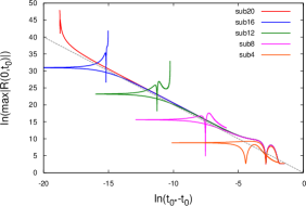
Figure 1: $m=0$ A data: $\ln|R(t,0)|$ against $\ln|t_{*0}-t_{0}|$ for a few supercritical (top) and subcritical (bottom) evolutions. These correspond to data investigated in adscollapsepaper and PretoriusChoptuik . The grey line represents $R(t,0)=|t_{*0}-t_{0}|^{-2}$, indicating that indeed the spacetime is CSS near the centre. In the labels, “sub$n$” means that $-\ln(p_{*}-p)=n$, and “super$n$” means $-\ln(p-p_{*})=n$.

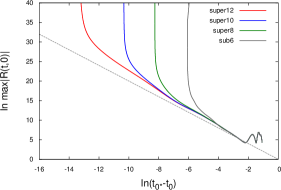
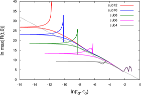
Figure 2: $m=1$ D data: the equivalent plots to Fig. 1.

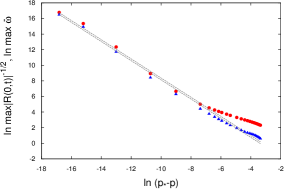
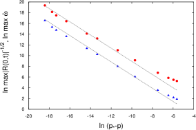
Figure 3: $m=0$ B (top) and C (bottom) data: power law scaling of $\max_{t}|R(t,0)|^{-1/2}$ (full red dots) and $\max_{t}\omega(t,0)$, against $p_{*}-p$. These maxima occur at $\bar{r}=0$. The grey dotted lines have slope $-\gamma=-1.23$ in both plots.

Figure 4: $m=1$ B (top) and D (bottom) families: power law scaling of $\max_{t}R(t,0)^{1/2}$ (red dots), $\max_{t,r}\bar{\omega}(t,r)$ (blue triangles) and the location in $\bar{r}$ of the maximum of $\bar{\omega}$ (blue empty triangles). The slope of all fitting lines is $-\gamma=-1.93$, with the vertical offset fitted individually (and clearly differing between the two families).

Figure 5: $m=2$ B (top) and C (bottom) data: power law scaling of $\max_{t,r}R(t,r)^{1/2}$ (red dots), $\max_{t,r}\bar{\omega}(t,r)$ (blue triangles) and the location in $\bar{r}$ of the maxima of $R$ (red empty dots) and $\bar{\omega}$ (blue empty triangles).

Figs. 1 and 2 provide evidence for the behaviour (70) and (72) for the $m=0$ A and $m=1$ D families of initial data, by showing $\ln R(t,0)$ against $\ln|t_{0}-t_{0*}|$.

In asymptotically flat spacetime, $f_{-}$ has a single maximum before decaying to zero. This means that, for subcritical ($p<p_{*}$) data

$$\max_{t}|R(t,0)|\simeq bA^{2}(p_{*}-p)^{-2\gamma},$$ (73)

where $A$ is again the same family-dependent constant as in (71,72) and $b:=\max f_{-}$ is a universal dimensionless constant GarfinkleDuncan . [This is a more explicit version of (15) above.] In our investigation adscollapsepaper of the $m=0$ case, we found that $f_{-}$ had two maxima and two minima before the final blowup. We could demonstrate scaling of both the values, and the location in $t_{0}-t_{0*}$, of all these extrema. Similar scaling laws hold for other geometric invariants, such as $\omega$ defined in (27), for which self-similarity predicts

$$\omega_{\rm max}\sim(p_{*}-p)^{-\gamma}.$$ (74)

For $\omega$ we only find a single maximum.

Fig. 3 gives evidence of these scaling laws for the $m=0$ B and C families, Fig. 4 for the $m=1$ B and D families, and Fig. 5 for the $m=2$ B and C families.

For quantities which vanish identically at the centre, such as the Ricci scalar for $m\geq 2$, or the angular momentum density $\omega$ for any $m$, we look for the maximum over all $r$ for a given $t$ instead, and plot this against $t_{0}-t_{0*}$. The resulting function of $t$ clearly depends on the time slicing, but seems to scale anyway, see again Figs. 4 and 5.

Table 1 shows the value of the Ricci scaling exponent $2\gamma$ for our 12 families of initial data. For $m=0$, $\gamma$ is the same for all families, as one would expect if there was a unique CSS solution with a single unstable mode. Strikingly, for $m>0$, $\gamma$ depends strongly on the family.

Beyond looking at the behaviour of the global maxima of $R$ and $\omega$, or the behaviour of their maxima over $r$ as a function of $t$, we have also attempted to look for direct evidence of self-similarity as a function of $(r,t)$, as we did successfully in adscollapsepaper for the $m=0$ case. We have constructed double-null coordinates $\tilde{u}$ and $\tilde{v}$ normalised to be proper time at the origin and with their origins fixed so that $\tilde{u}=\tilde{v}$ at the centre and $\tilde{u}=\tilde{v}=0$ at the accumulation point $t=t_{*}$. We can then define coordinates adapted to the self-similarity as $T:=-\ln(-\tilde{u})$ and $x:=\tilde{v}/\tilde{u}$, and plot against these coordinates. Quantities such as $\phi^{2}+\psi^{2}$, $e^{-T}\omega$, $M$, $R^{-2T}$ should then be functions of $x$ only in any self-similar region. However, the only quantity for which this works is the Ricci scalar. For this reason, we do not show any plots of, for example, the scalar field.

V.3 EMOTS location

As already discussed above, the AH is the curve in the $tr$ plane defined by ${\bar{r}}_{,v}=0$ , so that every point on it is a MOTS. As in adscollapsepaper , we denote a local minimum of $t_{\rm AH}(r)$ as an earliest MOTS (EMOTS). If there are two (or more) EMOTS, then in adscollapsepaper we denoted the earliest of these as the first MOTS (FMOTS), but we did not find this behaviour for $m>0$.

We focus here on the dependence of the entire AH curve, and the EMOTS location as one aspect of this, as a function of the parameter $p$, taking the example of the $m=1$ A data. A MOTS is already contained in the initial data for $p\gtrsim 0.74$. Reducing $p$ from this value, the location of the EMOTS moves inwards on an approximately null curve, then moves outwards very rapidly in $p$ in a spacelike direction at $p=p_{\rm break}\simeq 0.445465$, then moves to the future on a timelike curve, a little inwards again and then outwards again on an approximately null curve. Fig. 6 illustrates this for the range $0.74>p>0.404$.

Fig. 7 shows how this comes about, by showing the AH curve for selected values of $p$, with the lower plot zooming in on $p_{\rm break}$. For all $p$, there is only a single EMOTS, but the nature (timelike/spacelike) of the AH curve for the $m=1$ A data varies with $p$ in a complicated way.

For $p\simeq p_{\rm break}$ the AH curve has a section that is almost parallel to the time slices, and the local minimum moves along that shallow section very quickly, giving rise to the apparent jump in Fig. 6. This behaviour of the EMOTS is highly slicing-dependent.

For $p<p_{\rm break}$, the EMOTS mass does not scale. This is reminescent of the $m=0$ A data investigated in detail in adscollapsepaper : in that case there were two EMOTS, with a discontinuous switch from the inner to the outer EMOTS being the FMOTS. Only the inner EMOTS scaled.

Fig. 8 shows the EMOTS trajectory for the $m=1$ C data. This is much simpler, and the transition from the ingoing null to the timelike segment is now clearly continuous.

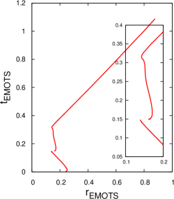
Figure 6: $m=1$ A data: the trajectory of the EMOTS location in the $tr$ plane, for values of the scalar field amplitude $p$ from $0.74$ (bottom) to $0.405$ (top). The $r$ and $t$ axes are drawn to the same scale so that null curves are at 45 degrees. The inset shows the timelike segment of the curve. We believe that the curve is actually continuous where there appears to be a break.

Figure 7: $m=1$ A data: the top plot shows the AH for representative values of $p$, namely $p=0.405$, $0.41$, $0.415$, $0.435$, $p_{\rm break}\simeq 0.445465$, $0.46$ and $0.5$ (from top to bottom). The bottom plots shows values of $p$ closer to $p_{\rm break}$, namely $p=0.445460$, $\dots 66$, $68$, $694$, $70$, $72$, $80$ (from top to bottom).

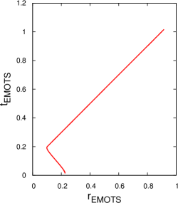
Figure 8: $m=1$ C data: the trajectory of the EMOTS location in the $tr$ plane, for values of the scalar field amplitude $p$ from $0.07$ (bottom) to $0.044$ (top). The extended timelike segment is not present for this family of initial data.

V.4 EMOTS mass and angular momentum

A key observation is that for $m=0$ there is a single critical value $p_{*}$ governing both subcritical and supercritical scaling, while for $m>0$ we have very different critical values of $p$ for subcritical scaling of the maximum of the Ricci scalar, and for scaling of the EMOTS mass, with $p_{*M}<p_{*}$. This means that both cannot be controlled by the same critical solution (in contrast to the $m=0$ case, where we have a theoretical model for this that also predicts the critical exponents).

For $m>0$, the evidence for supercritical EMOTS mass scaling is even weaker than for subcritical $R$ and $\omega$ scaling, and for the EMOTS angular momentum we have not found any scaling. Therefore, in the following, we do not show log-log plots of $M$ and $J$ against $p$, but show $p$ on a linear scale. As for the subcritical scaling of $R$ and $\omega$, the supercritical scaling of $M_{\rm EMOTS}$ does not continue to arbitrarily small scales for $m>0$. The mass scaling exponents, and the ranges of $\ln(p-p_{*M})$ for which we observe approximate power-law behaviour, are listed in Table 1. Like $\gamma$, the mass scaling exponent $\delta$ depends strongly on the family of initial data.

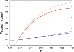
Figure 11: $m=1$ C data: the equivalent plots to Fig. 10. In contrast to the $m=1$ B data, we find subcritical but not supercritical scaling.

In Figs. 9-13 we give a few examples of the behaviour of the EMOTS mass and angular momentum, and the maxima of $R$ and $\omega$, as functions of the amplitude $p$, over a large range of $p$. We also indicate the approximate ranges of $p$ where we see supercritical and subcritical scaling. In these plots, the upper end of the plotting range for $p$ corresponds to a MOTS being present already in the initial data. The mininum of $p$ on the $M_{\rm EMOTS}$ curve corresponds to the EMOTS location having gone back out almost to outer boundary at $t\sim 1$ (compare Figs. 6 and 8), which however in $p$ is very close to $p_{*M}$. The lower end of the plotting range for $p$ corresponds to the lowest value of $p$ where we can clearly see a maximum of $R$ for some $t<2$. (Finding the maximum becomes numerically very difficult, and so it is not clear for all $p$ if one exists.)

As a reminder of the behaviour we found for the $m=0$ case in adscollapsepaper , Fig. 9 shows this for the $m=0$ B data. (For $m=0$ there is no angular momentum, but these initial data are complex, so instead of $\omega$ we show the “charge density” $\bar{\omega}$.) This illustrates that for $m=0$ there is a single value $p_{*}$ controlling both supercritical and subcritical scaling.

Figs. 10-12 then show three different families of initial data for $m=1$. The obvious difference to $m=0$ is that we now have separate critical values $p_{*}$ for subcritical scaling and $p_{*M}$ for supercritical scaling, with $p_{*}>p_{*M}$ for all $m>0$ data we have investigated. Moreover, the blowup of $\max R$ and $\max\omega$ at $p=p_{*}$ is immediately obvious (and power-law scaling is then confirmed by log-log plots such as Figs. 3-5), whereas the mass scaling is much less clear both by eye and in log-log plots.

Finally, Fig. 13 shows an example of an $m=2$ family of initial data, namely the $m=2$ B data.

An additional key difference between $m=0$ and $m>0$ is that for $m=0$, both super and subcritical scaling continues down to very small scales: the lower cutoff is either the (small) length scale set by the cosmological constant, or appears to be a lack of numerical resolution. In contrast, for $m>0$ scaling seems to end at some smallish scale for dynamical reasons that we do not yet understand. Looking at Table 1, we see that we observe EMOTS mass scaling only over about 3 $e$-foldings in $|p-p_{*}|$ for all $m>0$ data, in contrast to up to 10 $e$-foldings for $m=0$. We see Ricci scaling for up to 20 $e$-foldings in $|p-p_{*}|$ for $m=0$, but the “best” we have found for $m>0$ is 9 $e$-foldings. We have no real explanation for this failure of scaling at small scales, and can only guess that it is covered up by the infall of matter into the self-similar region of spacetime.

Among our three examples of $m>0$ families of data, we have selected $m=1$ D because it shows the clearest subcritical scaling (see Table 1, and the lower part of Fig. 4). By contrast, $m=1$ B (Fig.10) shows no subcritical scaling at all, while $m=1$ C (Fig.11) shows no supercritical scaling. We can only guess that these are extreme examples of infalling matter covering up what would otherwise be a self-similar region.

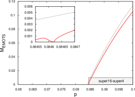
Figure 9: $m=0$ B data: the upper plot shows the EMOTS mass (red) and total mass (grey) against $p$. The inset shows the FMOTS location jump due to the presence of an inner EMOTS formed later in time (compare with Fig. 6 of adscollapsepaper ). The lower plot shows $\max_{t}R(t,0)$ (red) and $\max_{t,r}\bar{\omega}(t,r)$ (blue) against the same range of $p$. Note that $p_{*M}=p_{*}$ for this and all other $m=0$ families only. The shaded grey strips on the $p$-axis indicate the approximate ranges of $p$ where we observe scaling, with the text in these strips also indicating the corresponding range of $-\ln(p-p_{*M})$ and $-\ln(p_{*}-p)$, respectively.

There appears to be no supercritical scaling of $J$ at all for any of our ($m>0$) families. Again we have no explanation for this. Note that the mass that scales (and which we are using in all our plots) is the generalised Hawking mass $M_{\rm H}$ (based on the area radius, and becoming the irreducible mass of an isolated horizon or black hole), not the generalised BTZ mass $M_{\rm BTZloc}$ (which includes angular momentum, and becomes the BTZ mass of a black hole).

V.5 Numerical error

As an indication that the resolution-dependent numerical error is small, Fig. 14 shows approximate power-law scaling of the maximum of the Ricci scalar against $p_{*}-p$ for 1000 and 2000 grid points in $r$, with $\Delta r/\Delta t=1/4$ at both resolutions, for the $m=2$ B data (see below for what these data are). Adjusting $p_{*}$ so that the log-log plot approaches a straight line as much as possible, we find $p_{*}=0.871\pm 0.001$ at both resolutions, with no clear difference between the value at the two resolutions.

The main systematical error that we are aware of is a failure of our time evolution scheme to maintain the regularity condition $A=B$ at the centre $r=0$, at times shortly before the blowup. (In 2+1, blowup occurs very soon after maximum curvature, as measured by the time coordinate $t$, even for subcritical data). However, neither the EMOTS nor the maxima of $R$ and $\omega$ occur in the domain of dependence of the constraint violation, and so we believe their values are not affected.

VI Discussion

Going from the spherically symmetric scalar field in 3+1 dimensions with $\Lambda=0$ Choptuik1993 ; GundlachLRR , via the spherically symmetric scalar field in 2+1 dimensions with $\Lambda<0$ PretoriusChoptuik ; adscollapsepaper , to the rotating axisymmetric scalar field in 2+1 dimensions with $\Lambda<0$ (this work) the results of numerical time evolutions become more complicated and less well understood. Hence we begin this discussion by reviewing the two simpler situations.

In the 3+1 case with $\Lambda=0$ there is a clearly defined collapse threshold $p=p_{*}$: essentially all scalar field matter that does not immediately go into making the black hole escapes to infinity instead. For arbitrary 1-parameter families of initial data, with sufficient fine-tuning one can make the curvature arbitrarily large as $p\nearrow p_{*}$, and the black hole mass arbitrarily small as $p\searrow p_{*}$.

In the 2+1 case we need $\Lambda<0$ to form a black hole from regular initial data at all. This means that we effectively have a reflecting timelike outer boundary. As a consequence, all matter eventually falls into the black hole. In 2+1 dimensions with $\Lambda<0$ there is also a gap in the (dimensionless) mass between the adS ground state with $M=-1$, and the black hole solutions with $M>0$. [The range $-1<M\leq 0$ corresponds to point particles (conical singularities), which cannot form in collapse.]

For both these reasons the collapse threshold in 2+1 dimensions is less clearly defined than in higher dimensions: the final black hole mass is just the total mass $M_{\rm tot}$, as long as $M_{\rm tot}>0$, while for $M_{\rm tot}<0$ a black hole cannot form. (By contrast, in higher dimensions with $\Lambda<0$ there is still a reflecting boundary condition, but now the mass has dimension, there is no mass gap, and there is a well-defined threshold of black-hole formation after $0,1,2,\dots$ reflections at the outer boundary BizonRostworowski .)

In response to these features of 2+1 dimensions, we have adopted the approach of PretoriusChoptuik : we define as subcritical any evolution where the Ricci scalar reaches a local maximum (at the centre) before blowing up. We also do not measure the final black hole mass but the mass of the first intersection of the apparent horizon with our time slicing (the “earliest marginally outer-trapped surface”, or EMOTS).

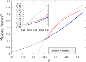
Figure 10: $m=1$ B data: the equivalent plots to Fig. 9, except that now $\max\omega$ is shown instead of $\max\bar{\omega}$, and $-J_{\rm EMOTS}/\ell$ is also shown. The EMOTS angular momentum (blue) is almost all of the total angular momentum (black dotted), and not surpringly does not show scaling. The EMOTS mass (red) is not much below the total mass (gray dotted), but does show scaling. We have not found any clear subcritical scaling. We believe this is “covered up” by other features of the time evolution.

In adscollapsepaper we found empirically that for $p\simeq p_{*}$ the time it takes for a light ray to reach the outer boundary and come back ($\Delta t\sim 2$ in our choice of coordinates) corresponds to an exponentially small proper time at the centre. This means that any outgoing radiation is scattered back to the centre almost immediately, in terms of the relevant time at the centre, and is probably why even in what we define as subcritical evolutions, a spacelike central curvature singularity develops very soon after the maximum of the Ricci scalar.

The system investigated in PretoriusChoptuik ; adscollapsepaper is the case $m=0$ with real $\Phi$ of this work, and the particular initial data used to produce all plots in adscollapsepaper corresponds to the A family of initial data here. For $m=0$, we found a critical value $p_{*}$ of $p$ at which both the maximum of Ricci becomes arbitrarily large as $p\nearrow p_{*}$, and the (inner) EMOTS mass arbitrarily small as $p\searrow p_{*}$. We identified a continuously self-similar (CSS) critical solution both theoretically and numerically. Based on this, we derived the Ricci scaling exponent $\gamma$ and mass scaling exponent $\delta$, in agreement with our numerical time evolutions.

There are some similarities between $m=0$ and $m>0$:

1. For most families of initial data, there is a threshold $p_{*M}$ such that the EMOTS mass shows power-law scaling as $p\searrow p_{*}$.

2. For most families of initial data, there is a threshold $p_{*}$ such that the Ricci scalar shows power-law divergence as $p\nearrow p_{*}$.

3. For initial data with $p\simeq p_{*}$, the maximum of the Ricci scalar evolves as a function of proper time at centre $t_{0}$ in a way that is compatible with the existence of a CSS solution with one unstable mode – the “standard” scenario for type-II critical collapse GundlachLRR .

However, key aspects of $m>0$ also differ from $m=0$ (see Table 1):

1. The critical values of $p$ for Ricci scaling and EMOTS scaling are widely separated (with $p_{*}>p_{*M}$ in all cases).

2. We observe both mass scaling and Ricci scaling only over a limited range of scales.

3. The scaling exponents $\gamma$ and $\delta$ depend strongly on the family of initial data.

4. With the exception of the Ricci scalar $R$, we have not convincingly been able to identify a CSS or DSS spacetime-dependence of relevant scalars such as $M$, $\phi^{2}+\psi^{2}$ or $\omega$ in evolutions for $p\simeq p_{*}$.

A strong motivation for this work was that in 2+1 spacetime dimensions axisymmetry (with rotation) is numerically almost as straightforward as spherical symmetry, and that the threshold of gravitational collapse with angular momentum has hardly been studied yet. We have made the following observations concerning angular momentum:

1. At least for some families, the maximum of the local angular momentum density $\omega$ shows subcritical scaling with the same (family-dependent) $\gamma$ as the maximum of $R$.

2. However, where this is the case the constant ratio $\max R/\max\omega^{2}$ depends on the family of initial data.

3. The previous two observations also hold for the “charge density” $\bar{\omega}:=\omega/m$ for $m=0$, where there can be no angular momentum.

4. The angular momentum of the EMOTS shows no critical scaling.

5. The bound $J<M\ell$ that applies to a BTZ black hole formed in collapse appears to also hold for the EMOTS. It appears to become sharp as $p\searrow p_{*M}$ for some but not all families of initial data.

It is hard to reconcile all this conflicting evidence. We are tempted to dismiss the EMOTS mass as an “epiphenomenon” that even for $m=0$ is somewhat gauge-dependent and not deeply coupled to the nonlinear dynamics adscollapsepaper . In particular, for $m>0$, the AH is no longer constrained to be spacelike, and we have seen that it can change shape with $p$ in a rather complicated way. However, the key observation for $m>0$ is simply that $p_{*M}$ is so different from $p_{*}$: this seems to rule out a scenario where the same critical solution controls both Ricci and EMOTS mass scaling.

There is no such argument for also dismissing the Ricci and $\omega$ scaling. We clearly see some threshold behaviour as $p\nearrow p_{*}$, and it may be that it ends at some level of fine-tuning (or is absent in a few families) only because the blowup associated with a critical solution is covered up by other, non-critical, dynamics.

If we take observations 2, 8, 9 and 10 seriously, and somehow explain observation 7 away as scaling behaviour being “covered up”, the least implausible theoretical model appears to be one where the dynamics as $p\nearrow p_{*}$ with $m>0$ is controlled by a family of asymptotically CSS solutions, maybe having more than one unstable mode, and admitting different angular momentum (or “charge”) to mass ratios. A toy model for this may be the competition between a real DSS and a complex CSS solution in a harmonic map coupled to gravity Liebling .

The obvious next step is to look for these critical solutions. From the experience with $m=0$ adscollapsepaper , a thorough study of asymptotically CSS solutions for $m>0$ is bound to be complex, and we leave this to future work.

Figure 12: $m=1$ D family: the equivalent plots to Fig. 10. This is the family where we see subcritical scaling over the largest range of $\ln(p_{*}-p)$ (see the lower plot of Fig. 4).

Figure 13: $m=2$ B family: $M_{\rm EMOTS}$, $J_{\rm EMOTS}$, $\ln R$ and $\ln\omega$ versus $p$.

Figure 14: Ricci scaling for the $m=2$ B data, as in Fig. 5, but with $\Delta r=1/1000$ (blue) and $\Delta r=1/2000$ (red). A best fit by eye gives $p_{*}=0.871\pm 0.001$ at the higher resolution, and we have used $p_{*}=0.871$ at both resolutions.

Appendix A Gauge freedom

To find the residual gauge freedom in the ansatz (5), we define the auxiliary coordinates

$$u:=t-r,\quad v:=t+r.$$ (75)

The metric becomes

$$ds^{2}=-f\,du\,dv+{\bar{r}}^{2}\left(d\theta+\beta{dv+du\over 2}\right)^{2}.$$ (76)

Consider now the coordinate transformation

$$u=u(\hat{u}),\quad v=v(\hat{v}),\quad\theta=\hat{\theta}+\vartheta(\hat{u},\hat{v}).$$ (77)

For the metric in $(\hat{u},\hat{v},\hat{\theta})$ to retain the form (76), we must have

$$\hat{\beta}=\beta{du\over d\hat{u}}+2\vartheta_{,\hat{u}}=\beta{dv\over d\hat{v}}+2\vartheta_{,\hat{v}}.$$ (78)

The sum and difference of these two PDEs give

$$\hat{\beta}={\beta\over 2}\left({du\over d\hat{u}}+{dv\over d\hat{v}}\right)+\vartheta_{,\hat{t}},$$ (79)

where $\vartheta$ is given by

$$\vartheta(\hat{t},\hat{r})=\vartheta_{\infty}(\hat{t})+\int_{\infty}^{\hat{r}}{\beta\over 2}\left({du\over d\hat{u}}-{dv\over d\hat{v}}\right)\,d\hat{r}^{\prime}.$$ (80)

Under the same gauge transformation,

$$\hat{f}=f{du\over d\hat{u}}{dv\over d\hat{v}}.$$ (81)

The three arbitrary functions of one variable $u(\hat{u})$, $v(\hat{v})$ and $\vartheta_{\infty}(\hat{t})$ precisely parameterise the residual gauge freedom of (76) and hence (5).

As we shall see below in Eq. (10), modulo Eq. (6), the metric coefficient $f$ obeys a wave equation with principal part $f_{,uv}$. Appropriate local data for this wave equation would be the value of $f$ on two null surfaces $(u=u_{0},v>v_{0})$ and $(v=v_{0},u>u_{0})$. From (81), these null data precisely fix the functions $\hat{u}(u)$ and $\hat{v}(v)$, so $f$ (or equivalently $A$) is pure gauge. The function $\vartheta_{\infty}(\hat{t})$, which parameterises a rigid time-dependent rotation of the coordinate system, can be fixed independently by setting $\beta(t,\pi\ell/2)$. We set

$$\beta(\pi\ell/2,t)=0,$$ (82)

which is the natural choice for asymptotically adS spacetimes.

Appendix B The Kerr-adS solution

Here we show that a horizon-crossing patch of the Kerr-adS metric can be written in the form (5).

In Schwarzschild-like coordinates $({\bar{t}},{\bar{r}},\theta)$, the eternal exterior Kerr-adS vacuum metric is given by

$$ds^{2}=-\bar{f}\,d{\bar{t}}^{2}+\bar{f}^{-1}\,d{\bar{r}}^{2}+{\bar{r}}^{2}(d\bar{\theta}+\bar{\beta}\,d{\bar{t}})^{2},$$ (83)

where the area radius ${\bar{r}}$ is used as a coordinate, and the metric coefficients $\bar{f}$ and $\bar{\beta}$ are given by BTZ ; Carlip

$$\bar{f}({\bar{r}}):=-M+{{\bar{r}}^{2}\over\ell^{2}}+{J^{2}\over 4{\bar{r}}^{2}},\quad\bar{\beta}({\bar{r}}):=-{J\over 2{\bar{r}}^{2}}.$$ (84)

The dimensionless mass parameter $M$ takes value $-1$ (with $J=0$) for adS spacetime, $-1<M\leq 0$ for a point particle/naked singularity and $M>0$ for a black hole. $J$ is the angular momentum of the spacetime. For $0<J^{2}/\ell^{2}<M^{2}$, $f=0$ has two roots $0<{\bar{r}}_{-}<{\bar{r}}_{+}<\infty$, corresponding to an inner and outer horizon.

Defining the tortoise coordinate ${\tilde{r}}({\bar{r}})$ for ${\bar{r}}>{\bar{r}}_{+}$ by

$${\tilde{r}}:=\int\bar{f}^{-1}\,d{\bar{r}},$$ (85)

(83) becomes

$$ds^{2}=\bar{f}(-d{\bar{t}}^{2}+d{\tilde{r}}^{2})+{\bar{r}}^{2}(d\bar{\theta}+\bar{\beta}\,d{\bar{t}})^{2},$$ (86)

which is of the form (5), with ${\bar{r}}$ now a function of ${\bar{t}}$ and ${\tilde{r}}$.

In terms of the auxiliary coordinates

$$U:={\bar{t}}-{\tilde{r}},\quad V:={\bar{t}}+{\tilde{r}},$$ (87)

both branches of the bifurcate outer horizon can be brought to finite coordinate values $u=0$ or $v=0$ by introducing the Kruskal coordinates

$$u:=-e^{-a_{+}U},\quad v:=e^{a_{+}V},$$ (88)

where the constant $a_{+}$ is determined by the requirement that $f$ is finite on the horizon. Further details can be found in BTZ ; Carlip . With $t$ and $r$ then defined by (75), and $\vartheta$ given by (80), the new metric again has the functional form (5), but is now finite on the horizon, with $\beta$ and $f$ given by (79,81).

The precise expressions for $f$, ${\bar{r}}$ and $\beta$ as functions of $(t,r)$ do not matter to us here, because in collapse simulations the BTZ metric will not appear in this specific form, but in a generic form related by a further regular coordinate transformation of the form (77). Our task is then to read off $M$ and $J$ when the BTZ metric, or a piece of it, is given in generic coordinates of the form (5).

Appendix C SBP finite differencing in $r$ for the wave equation

We assume here that the grid is centred and equally spaced, so that $r_{i}=i\Delta r$ for $i=0\dots N$. We finite-difference (63,64) as

$$\left(X_{,r}+\frac{p}{r}X\right)_{i}=$$

$${8(\tilde{X}_{i+1}I_{1}-\tilde{X}_{i-1}I_{-1})-(\tilde{X}_{i+2}I_{2}-\tilde{X}_{i-2}I_{-2})\over 12\bar{w}_{i}\Delta r},$$ (89)

$$\left(V_{,r}\right)_{i}={8(V_{i+1}-V_{i-1})-(V_{i+2}-V_{i-2})\over 12\Delta r},$$ (90)

where we have introduced the shorthands

$$I_{k}:=I(k,i,p):=\left(1+{k\over i}\right)^{p}$$ (91)

and

$$\tilde{X}_{0} \equiv 0,$$ (92)

$$\tilde{X}_{1} \equiv \tilde{v}_{1}X_{1}+u_{3/2}X_{2},$$ (93)

$$\tilde{X}_{2} \equiv \tilde{v}_{2}X_{2}+u_{3/2}X_{1}+u_{5/2}X_{3},$$ (94)

$$\tilde{X}_{3} \equiv \tilde{v}_{3}X_{3}+u_{5/2}X_{2},$$ (95)

$$\tilde{X}_{i} \equiv \tilde{v}_{i}X_{i},\qquad i\geq 4.$$ (96)

[These formulas are equivalent to Eqs. (57-65) of lwaveSBP , and are obtained from them by cancelling a factor of $i^{p}$ between numerator and denominator.] The coefficients $u_{3/2}$, $u_{5/2}$, $\bar{v}_{i}$ and $\bar{w}_{i}$ depend on the integer $p$ and are defined by a 4-th order recursion relation with boundary conditions at $i=0$ and $i\to\infty$.

While the stability of this scheme is not obvious, it is easy to see that with $\bar{v}_{i}=\bar{w}_{i}=1$, $u_{i}=0$, it reduces to applying the standard fourth-order accurate symmetric stencil to $X^{\prime}+pX/r=r^{-p}(r^{p}X)^{\prime}$, and is therefore a fourth-order accurate discretisation. The expression for $V^{\prime}$ is, just the standard symmetric 5-point 4-th order accurate finite difference, but it is important to note that the method consists of both finited-difference stencils, plus appropriate boundary conditions.

The symmmetry boundary $r=0$ is dealt with by extending the grid to two ghostpoints according to $X(-r)=-X(r)$ and $V(-r)=V(r)$. The outer boundary $r_{N}=\ell\pi/2$ is dealt with by one-sided finite differences for the last four grid points, namely

$$\left(X_{,r}+\frac{p}{r}X\right)_{N-3,\dots,N}=$$

$${8\tilde{X}_{N-5}I_{-2}-64\tilde{X}_{N-4}I_{-1}+59\tilde{X}_{N-2}I_{1}-3\tilde{X}_{N}I_{3}\over 98w_{N-3}\Delta r},$$

$${8\tilde{X}_{N-4}I_{-2}-59\tilde{X}_{N-3}I_{-1}+59\tilde{X}_{N-1}I_{1}-8\tilde{X}_{N}I_{2}\over 86w_{N-2}\Delta r},$$

$${-\tilde{X}_{N-2}I_{-1}+\tilde{X}_{N}I_{1}\over 2w_{N-1}\Delta r},$$

$${3\tilde{X}_{N-5}I_{-3}+8\tilde{X}_{N-2}I_{-4}-59\tilde{X}_{N-1}I_{-2}+48\tilde{X}_{N}\over 34w_{N}\Delta r}.$$

The corresponding one-sided finite differences for $V_{,r}$ use the same rational coefficients, but without the weights $v_{i},w_{i},I_{k}$.

We impose the boundary conditions $\phi,\phi^{\prime},V,V^{\prime},X=0$ and similarly $\psi,\psi^{\prime},W,W^{\prime},Y=0$ using the Olsson projection method Olsson , which is summarised in Appendix G of lwaveSBP . This method makes sure that the discrete energy estimate still holds after imposing the boundary conditions. It does not matter how we discretise the $r$-derivatives in these BCs, but we choose the $(3,8,-59,48)$ stencil for $d/dr$ at the boundary set out above.

The coefficients $\tilde{v}_{i}$ and $\tilde{w}_{i}$ are tabulated for $p=1,\dots,22$ (thus covering $m=0,\dots,10$), and for $i=0,\dots,2000$ in data . The asymptotic expansions

$$\tilde{v}_{i}^{(1)}=1$$ (101)

$$+ \frac{(2p-1)(p-1)p(p+1)(p+3)}{60i^{4}}$$

$$+ \frac{(2p-3)(p-3)(p-2)(p-1)p(p+1)(p+3)}{504i^{6}}$$

$$+ O(i^{-8})$$

and

$$\tilde{w}_{i}=1$$ (102)

$$+ \frac{(2p+1)(p+1)p(p-1)(p-3)}{60i^{4}}$$

$$+ \frac{(2p-1)(p-5)(p-3)(p-2)(p-1)p(p+1)}{504i^{6}}$$

$$+ O(i^{-8})$$

are accurate to double precision arithmetic for $i>2000$ and $p\leq 22$, thus complementing the tabulated values for arbitrarily large $i$.

References

- (1) J. R. Oppenheimer and H. Snyder. Phys. Rev. 56, 455 (1939).
- (2) M. W. Choptuik Phys. Rev. Lett. 70, 9, (1993).
- (3) C. Gundlach and J. M. Martín-García, Living Rev. Relativity, 2007-05 (2010).
- (4) D. Garfinkle and C. Gundlach, Class. Quantum Grav. 16, 4111 (1999).
- (5) A. M. Abrahams and C. R. Evans, Phys. Rev. D 49, 3998 (1994).
- (6) M. W. Choptuik, E. W. Hirschmann, S. L. Liebling and F. Pretorius, Phys. Rev. Lett. 93, 131101 (2004).
- (7) J. M. Martín-García and C. Gundlach, Phys. Rev. D 68, 024011, (2003).
- (8) F. Pretorius and M. W. Choptuik, Phys. Rev. D 62, 124012 (2000).
- (9) J. Jałmużna, C. Gundlach and T. Chmaj, Phys. Rev. D 92, 124044 (2015).
- (10) D. Garfinkle, Phys. Rev. D 63, 044007 (2001).
- (11) D. Garfinkle and G. C. Duncan, Phys. Rev.D 58, 064024 (1998).
- (12) R. M. Wald, General Relativity, University of Chicago Press, Chicago 1980.
- (13) C. Gundlach, J. M. Martín-García and D. Garfinkle, Class. Quantum Grav. 30, 145003 (2013).
- (14) P. Bizoń and A. Rostworowski, Phys. Rev.Lett. 107, 031102 (2011).
- (15) S. L. Liebling, Phys. Rev. D 58, 084015 (1998).
- (16) M. Bañados, C. Teitelboim and J. Zanelli, Phys. Rev. Lett. 69, 1849 (1992).
- (17) S. Carlip, Class. Quant. Grav. 12, 2853 (1995).
- (18) P. Olsson, Mathematics of Computation 64 1035-1065, (1995).
- (19) http://www.soton.ac.uk/cjg/lwaveSBP/.