Local Search for Minimum Weight Dominating Set with Two-Level Configuration Checking and Frequency Based Scoring Function

Abstract

The Minimum Weight Dominating Set (MWDS) problem is an important generalization of the Minimum Dominating Set (MDS) problem with extensive applications. This paper proposes a new local search algorithm for the MWDS problem, which is based on two new ideas. The first idea is a heuristic called two-level configuration checking (CC²), which is a new variant of a recent powerful configuration checking strategy (CC) for effectively avoiding the recent search paths. The second idea is a novel scoring function based on the frequency of being uncovered of vertices. Our algorithm is called CC²FS, according to the names of the two ideas. The experimental results show that, CC²FS performs much better than some state-of-the-art algorithms in terms of solution quality on a broad range of MWDS benchmarks.

1 Introduction

Given an undirected graph $G$, a dominating set $D$ is a subset of vertices such that every vertex not in $D$ is adjacent to at least one member of $D$. The Minimum Dominating Set (MDS) problem consists in identifying the smallest dominating set in a graph. The Minimum Weight Dominating Set (MWDS) problem is a generalized version of MDS. In the MWDS problem, each vertex is associated with a positive value as its weight, and the task is to find a dominating set that minimizes the total weight of the vertices in it.

The MWDS problem has played a prominent role in various real-world domains such as social networks, communication networks, and industrial applications. For example, Houmaidi et al. make the first known attempt to solve the sparse wavelength converters placement problem, where the MWDS problem is used to reduce the number of full wavelength converters in the deployment of wavelength division multiplexing all-optical networks (?). In the work of Subhadrabandhu, Sarkar, and Anjum (?), the MWDS problem is used in determining the nodes in an adhoc network where the intrusion detection software for squandering detection needs to be installed. Shen et al. propose a new method for multi-document by encoding this problem to the MWDS problem (?). Also, the problem of gateways placement, which places a minimum number of gateways such that quality-of-service requirements are satisfied, can be encoded into the MWDS problem and effectively solved by MWDS algorithms (?). An important problem in Web databases is to find an optimal query selection plan, which has been proved to be equivalent to finding a MWDS of the corresponding database graph (?).

The problems MDS and MWDS have been proved to be NP-hard (?, ?), which means that, unless P=NP, there is no polynomial-time algorithm for these problems. Several approximation algorithms have been introduced to solve the MWDS problem. An early constant-factor approximation algorithm for the MWDS problem in unit disk graphs is presented (?). A new centralized and distributed approximation algorithm for the MWDS problem is proposed with application to form a backbone for adhoc wireless networks (?). Dai and Yu propose a (5+$\varepsilon$)-approximation algorithm to form a MWDS for UDG (?). A (4+$\varepsilon$)-approximation dynamic programming algorithm for the MWDS problem is offered, which is the best approximation factor for unit disk graph without smooth weights (?). The first polynomial time approximation scheme for MWDS with smooth weights on unit disk graphs is introduced (?), which achieves a (1+$\varepsilon$)-approximation ratio, for any $\varepsilon$>0.

Nevertheless, as is usual, approximation algorithms with guaranteed approximation ratios do not have good performance in practice. Most practical algorithms for solving the MWDS problem are heuristic algorithms. In the work of Jovanovic, Tuba, and Simian (?), an ant colony optimization (ACO) algorithm for MWDS is proposed, which takes into account the weights of vertices being covered. An algorithm called ACO-PP-LS uses an ant colony optimization method by considering the pheromone deposit on the node and a preprocessing step immediately after pheromone initialization (?). A hybrid steady-state genetic algorithm HGA is proposed by using binary tournament selection method, fitness-based crossover and a simple bit-flip mutation scheme (?). In the work of Nitash and Singh (?), a swarm intelligence algorithm called ABC uses an artificial bee colony method to solve MWDS. A hybrid approach EA/G-IR is presented, which combines an evolutionary algorithm with guided mutation and an improvement operator (?). In the work of Bouamama and Blum (?), a randomized population-based iterated greedy approach R-PBIG is proposed to tackle MWDS, which maintains a population of solutions and applies the basic steps of an iterated greedy algorithm to each member of the population. However, the efficiency of existing heuristic algorithm are still not satisfactory, especially for hard and large-scaled instances (as will be shown in our experiments). The reason may be that the heuristic functions used in previous algorithms do not have enough information during the search procedure, and the cycling search problems can not be overcome by most algorithms as well.

In this paper, we develop a novel local search algorithm for the MWDS problem based on two new ideas. The first idea is a new variant of the Configuration Checking (CC) strategy. Initially proposed in the work of Cai, Su, and Sattar (?), the CC strategy aims to reduce the cycling phenomenon (i.e., revisiting candidate solutions which have been recently visited) in local search, by considering the circumstance of the solution components, which is formally defined as the configuration. The CC strategy has been successfully applied to a number of well-known combinatorial optimization problems, including Vertex Cover (?, ?, ?, ?), Set Covering (?, ?), Clique problem (?), Boolean Satisfiability (?, ?, ?, ?) and Maximum Satisfiability (?, ?), as well as application problems such as Golomb Rulers optimization (?). It is straightforward to devise the CC strategy for MWDS, which works as follows. For a vertex, it is forbidden to be added into the candidate solution if its configuration has not been changed after the last time it was removed from the candidate solution. However, when applied to the MWDS problem, the CC strategy does not lead to good performance. The problem may be that the original CC strategy is too strict for solving MWDS, i.e. forbidding too many vertices to be selected, which limits the search area of the algorithm. In this work, we propose a variant of the CC strategy based on a new definition of configuration. In this strategy, the configuration of a vertex $v$ refers to its two-level neighborhood, which is the union of the neighborhood $N(v)$ and the neighborhood of each vertex in $N(v)$. This new strategy is thus called two-level configuration checking (abbreviated as CC²).

The second idea is a frequency based scoring function for vertices, according to which the score of each vertex is calculated. Local search algorithms for the MWDS problem maintain a candidate solution, which is a set of vertices selected for dominating. Then the algorithms will use a scoring functions to decide which vertices will be selected to update the candidate solution, where the scores of vertices indicate the benefit (which may be positive or negative) produced by adding (or removing) a vertex to the candidate solution. Four greedy algorithms for the MWDS problem are developed by using four different scoring functions (?). After that, some scoring functions have been proposed recently (?, ?, ?, ?). These functions are mostly designed based on the information of the graph itself, for example vertex degree and vertex uncovered neighbour weight. An augmented cost function is designed, whose costs are either predetermined or evaluated during search (?). In this work, we also introduce a scoring function based on dynamic information of vertices, i.e., the frequency of being uncovered by the candidate solution. This scoring function exploits the information of the search process and that of the candidate solution. Moreover, different from the augmented cost function, our function does not have parameters and thus can be easily adapted to solve other optimization problems.

By incorporating these two ideas, we develop a local search algorithm for the MWDS problem termed CC²FS (as its two main ideas are CC² and Frequency-based Score). We carry out experiments to compare CC²FS with five state-of-the-art MWDS algorithms on benchmarks in the literatures including unit disk graphs and random generated instances, as well as two classical graphs benchmarks namely BHOSLIB (?) and DIMACS (?), and a broad range of real world massive graphs with millions of vertices and dozens of millions of edges (?). Experimental results show that CC²FS significantly outperforms previous algorithms and improves the best known solution quality for some difficult instances.

In the next section, we give some necessary background knowledge. After that, we propose a new configuration checking strategy CC², a frequency based scoring function, and a vertex selection method. Then, we propose a novel local search algorithm CC²FS, followed with experimental evaluations and analyses. Finally, we give concluding remarks.

2 Preliminaries

An undirected graph $G=(V,E)$ comprises a vertex set $V=\{v_{1},v_{2},\dots,v_{n}\}$ of $n$ vertices together with a set $E=\{e_{1},e_{2},\dots,e_{m}\}$ of $m$ edges, where each edge $e=\{v,u\}$ connects two vertices $u$ and $v$, and these two vertices are called the endpoints of edge $e$.

The distance between two vertices $u$ and $v$, denoted by $dist(u,v)$, is the number of edges in a shortest path from $u$ to $v$, and $dist(u,u)=0$ particularly. For a vertex $v$, we define its $i$th level neighborhood as $N_{i}(v)=\{u|dist(u,v)=i\}$, and we denote $N^{k}(v)=\bigcup_{i=1}^{k}N_{i}(v)$. The first-level neighborhood $N_{1}(v)$ is usually denoted as $N(v)$ as well, and we denote $N_{i}[v]=N_{i}(v)\cup\{v\}$. Also, we define the closed neighborhood of a vertex set S, $N[S]=\bigcup_{v\in S}N[v]$.

A dominating set of $G$ is a subset $D\subseteq V$ such that every vertex in $G$ either belongs to $D$ or is adjacent to a vertex in $D$. The Minimum Dominating Set (MDS) problem calls for finding a dominating set of minimum cardinality. In the Minimum Weight Dominating Set (MWDS) problem, each vertex $v$ is associated with a positive weight $w(v)$, and the task is to find a dominating set $D$ which minimizes the total weight of vertices in $D$ (i.e., min$\sum_{v\in D}w(v)$).

2.1 Local Search for MWDS

Local search algorithms perform the search on problem’s corresponding search space. The search space is implicitly defined by the way that the algorithm transforms a candidate solution into another. For the MWDS problem, local search algorithms usually maintain a candidate solution $S\subseteq V$ during the search. A vertex $v$ is covered by $S$ if $v\in N[S]$, and is uncovered otherwise. Also, the state of a vertex $v$ is denoted by $s_{v}\in\{1,0\}$, such that $s_{v}$=1 means a vertex $v$ is covered by a candidate solution $S$, and $s_{v}$=0 means it is uncovered. For a vertex, its age is defined as the number of steps since the last time it changed its state (being added or removed w.r.t. the maintained candidate solution $S$), and when we say the oldest vertex, we refer to the one with the minimum age value.

1

2$S:=InitFunction()$ and $S^{*}:=S$;

3 while not reach terminate condition do

4       if $S$ is better than $S^{*}$ then

5            $S^{*}:=S$;

6      $S:=MoveNeighbourPoisition(S)$;

7      

8return $S^{*}$;

Algorithm 1 The general framework of a local search algorithm

We first present a general framework of local search in Algorithm 1. As can be seen in this framework, the algorithm consists of two stage: the construction stage and the local search stage. At first, an initial dominating set is constructed by the greedy initialization process. After that, the solution is modified iteratively in the local search procedure, trying to find better solutions. In the local search stage, if a (redundant) dominating set is found, then the algorithm removes a vertex from $S$ and begins to search for a dominating set with smaller weight, until some stop criterion is reached. When the current candidate solution is not a dominating set, the move to a neighboring candidate solution consists of two phases: (1) removing a vertex from $S$ and (2) adding some vertices into $S$ until $S$ becomes a dominating set.

2.2 Configuration Checking

Local search suffers from the cycling phenomenon, i.e., revisiting a candidate solution that has been recently visited. This phenomenon wastes much computation time of a local search algorithm and more importantly prevents it from escaping from local optima.

To overcome the cycling problem, a number of methods have been proposed. The random walk strategy (?) picks the solution component randomly with a certain probability and greedily makes the best possible move with another probability. Random restarting (?) is used to restart the search from another starting point of search space. Also, allowing non-improving moves with a probability, as in the Simulating Annealing algorithm, can provide more diversification to the search. Glover proposes the tabu method (?), which has been widely used in local search algorithms (?, ?, ?). To prevent the local search to immediately return to a previously visited candidate solution, the tabu method forbids reversing the recent changes, where the strength of forbidding is controlled by a parameter called tabu tenure. Besides these general methods dealing with the cycling phenomenon, there are also heuristics specialized for problems, such as the promising decreasing variable exploitation for the Boolean Satisfiability (SAT) problem (?).

Recently, an interesting strategy called Configuration Checking (CC) (?) was proposed to handle the cycling problem in local search. Also, CC does not have instance-dependent parameters and is easy to use. The relationship between the tabu and CC strategy has been thoroughly discussed (?). If the tabu tenure is set to 1, it can be proved that given a variable, if it is forbidden to pick by the tabu method, it is also forbidden by the CC strategy, while its reverse is not necessarily true.

The MWDS problem is in some sense similar to the vertex cover problem in that their tasks are both to find a set of vertices. Thus, we can easily devise a CC strategy for the MWDS problem, following the one for the vertex cover problem (?). An important concept of the CC strategy is the configuration of vertices. Typically, the configuration of a vertex $v$ refers to a vector consisting of the states of all $v$’s neighboring vertices. The CC strategy for the MWDS problem can be described as following: given the candidate solution $S$, for a vertex $v\notin S$, if its configuration has not changed since $v$’s last removal from $S$, which means the circumstance of $v$ has not changed, then $v$ should not be added back to $S$.

An implementation of the CC strategy is to apply a Boolean array $confchange$ for vertices, where $confchange(v)$=1 means that $v$ is allowed to be added to $S$, and $confchange(v)$=0 on the contrary. In the beginning, for each vertex $v$, the value of $confchange(v)$ is initialized as 1; afterwards, when removing vertex $x$, $confchange(x)$ is set to 0; whenever a vertex $v$ changes its state, for each vertex $u\in N(v)$, $confchange(u)$ is set to 1.

3 Two-Level Configuration Checking

Since the CC strategy has been successfully applied to solve several NP-hard combinatorial optimization problems, a natural question arises whether this strategy can also be applied to MWDS. Unfortunately, a direct application of the original CC strategy in local search for the MWDS problem does not result in an effective algorithm, and has poor performance on a large portion of the benchmark instances.

We observe that, the original CC strategy would mislead the search by forbidding too many candidate vertices. In CC strategy, only the first-level neighborhood of a vertex is considered to avoid cycling, and the configuration of a vertex is considered changed only if at least one of its neighboring vertices changed its state. However, some analysis suggests that not only the first-level neighborhood but the second-level neighborhood are related to the cycling phenomenon and should be considered in the configuration of a vertex.

Inspired by this consideration, we propose a new variant of CC for MWDS, which is referred to as two-level configuration checking (CC² for short), by redefining the configuration of vertices. In the CC² strategy, we consider not only the first-level neighborhood ($N_{1}$) but also the second-level neighborhood ($N_{2}$).

3.1 Definition and Implementation of the CC² Strategy

In this subsection, we define the CC² strategy and present an implementation for it. We start from the formal definition of the configuration of a vertex $v$.

Definition 1.

Given an undirected graph $G=(V,E)$ and $S$ the candidate solution, the configuration of a vertex $v\in V$ is a vector consisting of state of all vertices in $N^{2}(v)$.

Based on the above definition, we can define an important vertex in local search as follows.

Definition 2.

Given an undirected graph $G=(V,E)$ and $S$ the candidate solution, for a vertex $v\notin S$, $v$ is configuration changed if at least one vertex in $N^{2}(v)$ has changed its state since the last time $v$ is removed from $S$.

In the CC² strategy, only the configuration changed vertices are allowed to be added to the candidate solution $S$.

We implement CC² with a Boolean array $ConfChange$ whose size equals the number of vertices in the input graph. For a vertex $v$, the value of $ConfChange[v]$ is an indicator — $ConfChange[v]$=1 means $v$ is a configuration changed vertex and is allowed to be added to the candidate solution $S$; otherwise, $ConfChange[v]$=0 and it cannot be added to $S$. During the search procedure, the $ConfChange$ array is maintained as follows.

CC²-RULE1. At the start of search process, for each vertex $v$, $ConfChange[v]$ is initialized as 1.

CC²-RULE2. When removing a vertex $v$ from the candidate solution $S$, $ConfChange[v]$ is set to 0, and for each vertex $u\in N^{2}(v)$, $ConfChange[u]$ is set to 1.

CC²-RULE3. When adding a vertex $v$ into the candidate solution $S$, for each vertex $u\in N^{2}(v)$, $ConfChange[u]$ is set to 1.

To understand RULE2 and RULE3, we note that if $u\in N^{2}(v)$, then $v\in N^{2}(u)$. Thus, if a vertex $v$ changes its state (i.e., either being removed or added w.r.t. the candidate solution), the $Configuration$ of any vertex $u\in N^{2}(v)$ is changed.

3.2 Relationship between CC and CC² Strategies

Configuration checking is a general idea, and both the original CC strategy and the CC² strategy are evolved from this idea. Both strategies prefer to pick configuration changed vertices. The difference between these two strategies lies on the concept of configuration changed vertices.

In the following, we compare these two kinds of configuration changed vertices. Let us use $CCV$ to denote the set of configuration changed vertices according to the original CC strategy, and use $CCV^{2}$ to denote the set of configuration changed vertices according to the CC² strategy.

Proposition 1.

Given an undirected graph $G=(V,E)$ and $S$ the maintained candidate solution, assuming that in some step $t$ we have $CCV=CCV^{2}$, then we can conclude that in the next step, for any $v\in V$, if $v\in CCV$, then $v\in CCV^{2}$.

Proof. Let us use $v^{*}$ to denote the vertex selected to change the state in step $t$ of the local search stage for MWDS. In step $t+1$, for any vertex $v$, we have two cases. 1) $v$ was in $CCV$ in step $t$. Since in step $t$ we have $CCV=CCV^{2}$, thus we also have $v\in CCV^{2}$; 2) $v$ was not in $CCV$ in step $t$. If $v\in CCV$ in step $t+1$, according to the definition of CCV, this can happen only when $v\in N[v^{*}]$. Because $N[v^{*}]\subset N^{2}[v^{*}]$, we also have $v\in N^{2}[v^{*}]$, and thus $v\in CCV^{2}$ in step $t+1$.

The above proposition gives an insight that the size of $CCV^{2}$ is larger than that of $CCV$. It is easy to see that the reverse of Proposition 1 is not necessarily true. So, we can easily deduce the following conclusion.

Remark 1 In most conditions, the $CCV^{2}$ set is a superset of $CCV$ set.

For an algorithm, in each step, there are more candidate vertices which could be added into the candidate solution under the CC² strategy than under the CC strategy. For this reason, we have more options and thus can explore more search spaces by choosing vertex from $CCV^{2}$ than from $CCV$.

4 A Novel Scoring Function for MWDS

Local search algorithms decide which vertex to be selected according to their scores. Thus, the scoring function for vertices plays a critical role in the algorithm, which has direct impact on the intensification and diversification of the search.

4.1 The Previous Scoring Function for MWDS

Recently, four scoring functions are presented to solve MWDS (?). We list the definitions of these score as below.

$\displaystyle{score_{1}(u)=\frac{d(u)}{w(u)}}$

$\displaystyle{score_{2}(u)=\frac{W(u)}{w(u)}}$

$score_{3}(u)=W(u)-w(u)$

$\displaystyle{score_{4}(u)=\frac{d(u)\times W(u)}{w(u)}}$

where $u\notin S$, $d(u)$ is the number of uncovered (non-dominated) neighbours of a given vertex $u$ and $W(u)$ is the sum of the weights of the uncovered neighbours of $u$.

The results of this experiment (?) show that the first, the second and the last heuristic functions result in a similar performance with no clear pattern of a particular greedy heuristic being better for general graph instances. In contrast, the third greedy heuristic clearly results in the poorest performance.

The weight of vertices being covered in $score_{2}$ is taken into account (?). In ACO-PP-LS (?), when a newly obtained solution may not be a dominating set, it is repaired by iteratively adding vertices from some vertices not in this obtained solution according to two strategies. With a certain probability, the first strategy is used, otherwise the second strategy is used. Specially, the first strategy is greedy and adds a vertex by using $score_{2}$, while the second strategy adds a vertex into the candidate solution randomly. ABC (?) prunes some redundant vertices according to the greedy strategy $score_{1}$. In EA/G-IR (?), there are two modifications in $score_{2}$. The first modification uses the closed neighborhood $N_{1}[u]$ instead of $N_{1}(u)$ when computing $score_{2}(u)$. The second modification is a tie-breaking rule. Actually, when there are more than one vertex satisfying $score_{2}$, then the next vertex to be added is selected by this tie-breaking rule. $score_{1}(u)$ is also computed by the closed neighborhood $N_{1}[u]$ and then the next vertex to be added is determined with this improved $score_{1}(u)$. In case there is still more than one vertices satisfying $score_{1}$, then the next vertex to be added is selected arbitrarily from these vertices. In R-PBIG (?), each vertex is rated based on greedy functions $score_{1}$ or $score_{2}$ and how to select which greedy function is based on a random number.

4.2 The Frequency based Scoring Function

In this paper, we introduce a novel scoring function by taking into account of the vertices’ frequency, which can be viewed as some kind of dynamic information indicating the accumulative effectiveness that the search has on the vertex. Intuitively, if a vertex is usually uncovered, then we should encourage the algorithm to select a vertex to make it covered.

In detail, in a graph, each vertex $v\in V$ has an additional property, frequency, denoted by $freq[v]$. The $freq$ of each vertex is initialized to 1. After each iteration of local search, the $freq$ value of each uncovered vertex is increased by one. During the search process, we apply the $freq$ of vertex to decide which vertex to be added or removed. Based on this consideration, we propose a new score function, which is formally defined as below.

Definition 3.

For a graph $G=(V,E)$, and a candidate solution $S$, the frequency based scoring function denoted by $score_{f}$, is a function such that

$$score_{f}(u)=\left\{\begin{aligned} \frac{1}{w(u)}\times\sum_{v\in C_{1}}freq[v],u\notin S,\\ -\frac{1}{w(u)}\times\sum_{v\in C_{2}}freq[v],u\in S,\end{aligned}\right.$$ (1)

where $C_{1}$=$N[u]\setminus N[S]$ and $C_{2}$=$N[u]$ $\setminus N[S\setminus\{u\}]$.

Remark that, in the above definition, $C_{1}$ is indeed the set of uncovered vertices that would become covered by adding $u$ into $S$ and $C_{2}$ is the set of covered vertices that would become uncovered by removing $u$ from $S$.

5 The Selection Vertex Strategy

During the search process, for preventing visiting previous candidate solutions, we not only use the CC² strategy in the adding process, but also use the forbidding list in the removing process. The $forbid\_list$ used here is a tabu list which keeps track of the vertices added in the last step, and these vertices are prevented from being removed within the tabu tenure. In this sense, this frequency based prohibition mechanism can be viewed as an instantiation of the longer term memory tabu search, and the main difference is that our method also consider the information from the $CC^{2}$ strategy.

The algorithm picks a vertex to add or remove, using the frequency based scoring function and the above two strategies. Firstly, we give two rules for removing vertices.

REMOVE-RULE1. Removing one vertex $v$, which has the highest value of $score_{f}(v)$, breaking ties by selecting the oldest one.

REMOVE-RULE2. Removing one vertex $v$, which is not in $forbid\_list$ and has the highest value of $score_{f}(v)$, breaking ties by selecting the oldest one.

When the algorithm finds a solution, it removes one vertex from the solution and continues to search for a solution with smaller weight. In this process, we use REMOVE-RULE1 to pick the vertex. During the search for a solution, the algorithm exchanges some vertices, i.e., removing one vertex from the candidate solution and then iteratively adding vertices into the candidate solution. In this case, we select one vertex to remove according to REMOVE-RULE2.

The rule to select the adding vertices is given below.

ADD-RULE. Adding one vertex $v$ with $ConfChange[v]\neq 0$, which has the greatest value $score_{f}(v)$, breaking ties by selecting the oldest one.

When adding one vertex into the candidate solution, we try to make the resulting candidate solution’s cost (i.e., the total weight of uncovered vertices) as small as possible. When adding one configuration changed vertex with the highest value $score_{f}(v)$, breaking ties by preferring the oldest vertex.

6 CC²FS Algorithm

Based on CC² and the frequency based scoring function, we develop a local search algorithm named CC²FS. During the process of local search, we maintain a set from which the vertex to be added is chosen. The set for finding a vertex to be removed from the candidate solution is simply $S$.

$CCV^{2}=\{v|ConfChange[v]=1,v\notin S\}$

The pseudo code of CC²FS is shown in Algorithm 2. At first, CC²FS initializes $ConfChange$, $forbid\_list$ and the $frequency$ and $score_{f}$ of vertices. Then it gets an initial candidate solution $S$ greedily by iteratively adding the vertex that covers the most remaining uncovered vertices until $S$ covers all vertices. At the end of initialization, the best solution $S^{*}$ is updated by $S$.

1

Input: a weighted graph $G=(V,E,W)$, the cutoff time

2

Output: dominating set of $G$

3

4initialize $ConfChange$, $forbid\_list$, and the $freq$ and $score_{f}$ of of vertices;

5 $S:=InitGreedyConstruction()$ and $S^{*}:=S$;

6 while elapsed time $<$ cutoff do

7       if there are no uncovered vertices then

8             if $w(S)<w(S^{*})$ then $S^{*}:=S$;

9            

10            $v:=$ a vertex in $S$ with the highest value $score_{f}(v)$, breaking ties in the oldest one;

11             $S:=S\setminus\{v\}$ and update $ConfChange$ according to CC²-RULE2;

12             continue;

13            

14      $v:=$ a vertex in $S$ with the highest value $score_{f}(v)$ and $v\notin forbid\_list$, breaking ties in the oldest one;

15       $S:=S\setminus\{v\}$ and update $ConfChange$ according to CC²-RULE2;

16       $forbid\_list:=\emptyset$;

17       while  there are uncovered vertices do

18             $v:=$ a vertex in $CCV^{2}$ with the highest value $score_{f}(v)$, breaking ties in the oldest one;

19             $S:=S\cup\{v\}$ and update $ConfChange$ according to CC²-RULE3;

20             $forbid\_list:=forbid\_list\cup\{v\}$;

21             $freq[v]:=freq[v]+1$, for $v\notin N[S]$;

22            

23      

24return $S^{*}$;

Algorithm 2 CC²FS ($G$, cutoff)

After initialization, the main loop from lines 3 to 16 begins by checking whether $S$ is a solution (i.e., covers all vertices). When the algorithm finds a better solution, $S^{*}$ is updated. Then one vertex with the highest $score_{f}$ value in $S$ is selected to be removed, breaking tie in favor of the oldest one. Finally, the values of $ConfChange$ are updated by CC²-RULE2.

If there are uncovered vertices, CC²FS first picks one vertex to remove from $S$ with the highest value $score_{f}$, breaking tie in favor of the oldest one. Note that when choosing a vertex to remove, we do not consider those vertices in $forbid\_list$, as they are forbidden to be removed by the forbidden list. After removing a vertex, CC²FS updates the $ConfChange$ values according to CC²-RULE2, and clear $forbid\_list$. Additional, since the tabu tenure is set to be 1, the $forbid\_list$ shall be cleared to allow previous forbidden vertices to be added in subsequent loop.

After the removing process, CC²FS iteratively adds one vertex into $S$ until it covers all vertices, i.e. the candidate solution is a dominating set. CC²FS first selects $v\in CCV^{2}$ with the greatest $score_{f}(v)$, breaking ties in favor of the oldest one. When the picked uncovered vertex is added into the candidate solution, the $ConfChange$ values are updated according to CC²-RULE3 and this added vertex is added into the $forbid\_list$. After adding an uncovered vertex each time, the frequency of uncovered vertices is increased by one. When the time limit reaches, the best solution will be returned.

Now we shall analyse the time complexity of CC²FS. For each iteration:

• The algorithm first dedicates to find a dominate set (Line 4-8). The worst time complexity for finding the removal vertex $v_{i}$ is $O(|S|)$ (Line 6), where $|S|$ denotes the size of the candidate solution $S$. Then, the algorithm updates the value of the related $score_{f}$ as well as $ConfChange$ (Line 10) and the worst time complexity is $O(\Delta(G)^{2})$, where $\Delta(G)=max\{|N[v]||v\in V,G=(V,E)\}$.

• Otherwise, the algorithm first decides which vertex $v_{j}$ should be deleted and the worst time complexity is also $O(|S|+\Delta(G)^{2})$ (Line 9-11). Let $L$ denote the number of uncovered vertices of $S$ (Line 12-16), and under the worst condition the step of the adding procedure is $L=|N[v_{j}]|$. During this adding procedure, the worst time complexity per step for adding one vertex is $O((|V|-|S|))$ (Line 13). When updating the related $score_{f}$ and $ConfChange$ (Line 14), the worst time complexity per step is also $O(\Delta(G)^{2})$. Then, the worst time complexity for the whole adding procedure (Line 12-16) is $O(|N[v_{j}]|(|V|-|S|+\Delta(G)^{2}))$.

Therefore, each iteration of the local search stage of CC²FS has a time complexity of $O(|S|+\Delta(G)^{2}+|N[v_{j}]|(|V|-|S|+\Delta(G)^{2}))=O(\Delta(G)^{2}+\Delta(G)(|V|-|S|+\Delta(G)^{2}))=O(max\{\Delta(G)|V|$, $\Delta(G)^{3}\})$.

7 Empirical Results

We compare CC²FS with five competitors on a broad range of benchmarks, with respect to both solution quality and run time. The run time is measured in CPU seconds. Firstly, we introduce the test instances, five competitors and the experimental preliminaries of our experiments.

There are eight benchmarks selected in our experiment, including T1, T2, UDG, two weighted versions of DIMACS, two weighted versions of BHOSLIB, as well as many real world massive graphs. We introduce the benchmarks in the following.

• T1 benchmark (?) (530 instances): all instances are connected undirected graphs with the vertex weights randomly distributed in the interval [20,70].

• T2 benchmark (?) (530 instances): the weight of all vertices in all instances is assigned as be a function based on the degree $d(v)$ of the vertex $v$ which is randomly set to in the interval [1, $d(v)^{2}$].

• UDG benchmark (?) (120 instances): these instances are generated by using the topology generator (?). Transmission range of all vertices in UDG instances is fixed to either 150 or 200 units.

• BHOSLIB benchmark with weighting function $w(v_{i})$=($i$ mod 200)+1 (41 instances): BHOSLIB instances (?) were originally unweighted and generated randomly based on the model RB (?, ?, ?).

• BHOSLIB benchmark with weighting function $w(v_{i})$=1 (41 instances): this benchmark is to test algorithms on uniform weight BHOSLIB graphs.

• DIMACS benchmark with weighting function $w(v_{i})$=($i$ mod 200)+1 (54 instances): DIMACS is the most frequently used for comparison and evaluation of graph algorithms. More specifically, the size of the DIMACS instances ranges from less than 150 vertices and 300 edges up to more than 4,000 vertices and 7,900,000 edges. We use the complement graphs of some instances, including the c-fat.clq and p-hat.clq set, to test the efficiency of our algorithm. The original DIMACS graphs are unweighted.

• DIMACS benchmark with weighting function $w(v_{i})$=1 (54 instances): this benchmark is to test algorithms on uniform weighted DIMACS graphs.

• Massive graph benchmark with weighting function $w(v_{i})$=($i$ mod 200)+1 (74 instances): these were transformed from the unweighted graphs in Network Data Repository online (?).

For T1, T2, UDG instances, we note that ten instances are generated for each combination of number of nodes and transmission range. As for the weighting function: for the $i$th vertex $v_{i}$, $w(v_{i})$=($i$ mod 200)+1, it was proposed in the work of Pullan (?) and has been widely used in the literature for algorithms for solving problems on vertex weighted graphs.

We compare CC²FS with HGA (?), ACO-PP-LS (?), ABC (?), EA/G-IR (?), and R-PBIG (?). Among them, R-PBIG and ACO-PP-LS are the best available algorithms for solving MWDS. We have the source code of ACO-PP-LS, so in this paper we use its code to test all benchmarks to get better solution values than those values (?).

We implement CC²FS in C++ and compile it by g++ with the -O2 option. All the experiments are run on Ubuntu Linux, with 3.1 GHZ CPU and 8GB memory. For T1, T2, and UDG instances, CC²FS and ACO-PP-LS are performed once, where one run is terminated upon reaching a given time limit. Among this, the parameter time limit is set to 50 seconds when the number of vertices is less than 500, otherwise the time limit is set to 1000 seconds. We report the real time $RTime$ of ACO-PP-LS and CC²FS, while we also give the finial execution time $FTime$ of EA/G-IR and R-PBIG. The real time is a time when ACO-PP-LS and CC²FS obtain the best solution respectively. The MEAN contains the average solution values for each of the ten instances of graphs of a particular size.

For DIMACS, BHOSLIB, and massive graphs instances, our algorithm and ACO-PP-LS are performed 10 independent runs with different random seeds, where each run is terminated upon reaching a given time limit 1000 seconds. The MIN and AVG column contains the minimal and average solution values for each instance by performing 10 runs with different random seeds. The SD column contains the standard deviation for each instance by performing 10 runs. The bold value indicates the best solution value among the different algorithms compared.

Note that for DIMACS, BHOSLIB, and massive graphs benchmarks, we only compare our algorithm with ACO-PP-LS. This is because, 1) as we mentioned, seen from the literatures, R-PBIG and ACO-PP-LS are the best available algorithms for solving MWDS; 2) we have the source code of ACO-PP-LS, while the source code of R-PBIG is not available to us.

7.1 Results on T1 and T2 Benchmarks

The performance results of previous algorithms on the T1 benchmark are displayed in Table 1. More importantly, this table also summarizes the experimental results on the first benchmark for our algorithm.

Among previous algorithms, for most instances, R-PBIG and ACO-PP-LS can find better solutions than HGA, ABC and EA/G-IR, with only a few exceptions.

For our algorithm, we show the minimum solution value and the run time. As is clear from the Table 1, CC²FS shows significant superiority on the T1 benchmark, except v50e750. By comparing these algorithms, we can easily conclude that CC²FS outperforms other algorithms.

The experimental results on the T2 benchmark are presented in Table 2. The quality of the solutions found by CC²FS is always much smaller than those found by other algorithms on all instances with 2 exceptions, i.e. v250e250 and v800e10000.

Table 1: Experiment results of HGA, ACO-PP-LS, ABC, EA/G-IR, R-PBIG, and CC²FS on the T1 benchmark. Each set contains 10 instances.

Instance	HGA	ACO-PP-LS		ABC	EA/G-IR		R-PBIG		CC2FS
T1	MEAN	MEAN	RTime	MEAN	MEAN	FTime	MEAN	FTime	MEAN	RTime
v50e50	531.3	531.3	0.2	534	532.9	0.21	531.3	0.5	531.3	<0.01
v50e100	371.2	371.2	0.17	371.2	371.5	0.23	371.1	0.8	370.9	<0.01
v50e250	175.7	175.7	0.12	175.7	175.7	0.18	175.7	1.3	175.7	<0.01
v50e500	94.9	94.9	0.05	94.9	94.9	0.16	95	2.3	94.9	<0.01
v50e750	63.1	63.1	0.03	63.1	63.3	0.1	63.8	2.5	63.3	<0.01
v50e1000	41.5	41.5	0.01	41.5	41.5	0.1	41.5	3	41.5	<0.01
v100e100	1081.3	1065.6	2.05	1077.7	1065.5	0.76	1061.9	1.4	1061	0.04
v100e250	626.2	623.1	1.3	621.6	620	0.72	619.3	2.2	618.9	0.04
v100e500	358.3	360.6	0.54	356.4	355.9	0.6	356.5	3	355.6	<0.01
v100e750	261.2	261	0.46	255.9	256.7	0.52	256.5	3.7	255.8	<0.01
v100e1000	205.6	207.3	0.38	203.6	203.6	0.49	203.6	4.3	203.6	<0.01
v100e2000	108.2	108.4	0.2	108.2	108.1	0.45	108	6.2	107.4	0.19
v150e150	1607	1582	4.88	1607.9	1587.4	1.64	1582.5	2.4	1580.5	0.02
v150e250	1238.6	1228.4	3.67	1231.2	1224.5	1.71	1219.5	3.3	1218.2	0.06
v150e500	763	763	2.2	752.1	755.3	1.45	745	4.3	744.6	0.05
v150e750	558.5	554	1.46	549.3	550.8	1.27	548.2	5.2	546.1	0.04
v150e1000	438.7	440.7	1.34	435.1	435.2	1.11	433.6	5.9	432.9	0.03
v150e2000	245.7	251.8	0.89	242.2	241.5	0.88	241.5	8.7	240.8	0.17
v150e3000	169.2	171.4	0.8	167.8	168.1	0.82	168.4	11.1	166.9	0.06
v200e250	1962.1	1919.5	9.54	1941.1	1924.1	3.68	1914.6	4.7	1910.4	0.19
v200e500	1266.3	1252.9	4.92	1246.9	1251.3	3.3	1235.3	6.2	1232.8	1.01
v200e750	939.8	934.3	3.71	923.7	927.3	2.78	914.9	7.4	911.2	0.45
v200e1000	747.8	741.8	2.99	730.4	731.1	2.39	725.2	8.2	724	0.25
v200e2000	432.9	437.3	1.36	417.6	417	1.68	414.8	10.9	412.7	0.45
v200e3000	308.5	308.8	1.24	294.4	294.7	1.42	294.2	14.2	292.8	0.41
v250e250	2703.4	2646.6	16.09	2685.7	2653.7	4.65	2653.7	6	2633.4	0.2
v250e500	1878.8	1840.1	10.91	1836	1853.3	4.66	1812.6	8.6	1805.9	0.92
v250e750	1421.1	1396.8	7.15	1391.9	1399.2	4.25	1368.6	9.6	1362.2	0.65
v250e1000	1143.4	1120.2	5.53	1115.3	1114.9	3.69	1097.1	10.9	1091.1	0.48
v250e2000	656.6	666	3.23	630.5	637.5	2.65	624.7	14	621.9	0.44
v250e3000	469.3	469.4	2.64	454.9	456.3	2.16	451.5	17.9	447.9	0.72
v250e5000	300.5	307	2.29	292.4	291.8	5.16	291.5	25.4	289.5	0.17
v300e300	3255.2	3190.6	24.39	3240.7	3213.7	8.73	3189.3	7.6	3178.6	1.47
v300e500	2509.8	2461.4	21	2484.6	2474.8	7.21	2446.9	10.2	2438.1	1.46
v300e750	1933.9	1885.1	16.91	1901.4	1896.3	6.48	1869.6	12	1854.6	1.6
v300e1000	1560.1	1532.7	10.49	1523.4	1531	5.7	1503.4	13.2	1495	0.61
v300e2000	909.6	900.5	5.95	875.5	880.1	4.03	872.5	16.8	862.5	1.93
v300e3000	654.9	658.8	4.03	635.3	638.2	3.27	629	21.3	624.3	1.12
v300e5000	428.3	432.3	3.67	411	415.7	2.59	409.4	29.8	406.1	1.72
v500e500	5498.3	5370.4	99.09	5480.1	5380.1	37.52	5378.4	21.1	5305.7	2.63
v500e1000	3798.6	3675.8	64.96	3707.6	3695.2	26.36	3642.2	29.1	3607.8	4.24
v500e2000	2338.2	2236.2	32.85	2266.1	2264.3	25.54	2203.9	36.1	2181	4.83
v500e5000	1122.7	1105.8	15.57	1070.9	1083.5	9.02	1055.9	55.9	1043.3	5.07
v500e10000	641.1	640.9	10.57	596	606.8	6.08	596.3	76.2	587.2	6.19
v800e1000	8017.7	7991.6	174.62	7907.3	7792.2	129.82	7768.6	67.9	7663.4	10.58
v800e2000	5317.7	5298.4	95.34	5193.2	5160.7	102.09	5037.9	83.3	4982.1	8.83
v800e5000	2633.4	2578.8	59.23	2548.6	2561.9	53.02	2465.4	122.6	2441.2	6.58
v800e10000	1547.7	1512.7	41.86	1471.7	1497	31.17	1420	171.1	1395.6	6.84
v1000e1000	11095.2	10984.9	412.14	10992.4	10771.7	249.82	10825	96.9	10585.3	12.18
v1000e5000	3996.6	3977.7	91.07	3853.7	3876.3	107.41	3693.1	184.2	3671.8	8.49
v1000e10000	2334.7	2291.8	83.82	2215.9	2265.1	63.22	2140.3	254.9	2109	9.43
v1000e15000	1687.5	1647.4	63.15	1603.2	1629.4	45.86	1549.1	282	1521.5	11.91
v1000e20000	1337.2	1297.5	44.21	1259.5	1299.9	36.35	1219	289.8	1203.6	11.4

Table 2: Experiment results of HGA, ACO-PP-LS, ABC, EA/G-IR, R-PBIG, and CC²FS on the T2 benchmark. Each set contains 10 instances.

Instance	HGA	ACO-PP-LS		ABC	EA/G-IR		R-PBIG		CC2FS
T2	MEAN	MEAN	RTime	MEAN	MEAN	FTime	MEAN	FTime	MEAN	RTime
v50e50	60.8	60.8	0.08	60.8	60.8	0.19	60.8	0.5	60.8	<0.01
v50e100	90.3	90.3	0.17	90.3	90.3	0.27	90.3	0.8	90.3	<0.01
v50e250	146.7	146.7	0.09	146.7	146.7	0.23	146.7	1.4	146.7	<0.01
v50e500	179.9	179.9	0.04	179.9	179.9	0.09	179.9	2.1	179.9	<0.01
v50e750	171.1	171.1	0.01	171.1	171.1	0.07	171.1	2.4	171.1	<0.01
v50e1000	146.5	146.5	0.01	146.5	146.5	0.06	146.5	2.9	146.5	<0.01
v100e100	124.5	123.5	1.05	124.4	123.5	0.6	123.5	1.2	123.5	<0.01
v100e250	211.4	210.1	0.89	209.6	209.2	0.92	209.2	2.1	209.2	<0.01
v100e500	306	305.7	0.57	305.8	305.7	0.78	305.7	2.9	305.7	<0.01
v100e750	385.3	384.5	0.45	384.5	384.5	0.7	386.9	3.5	384.5	<0.01
v100e1000	429.1	427.7	0.21	427.3	427.3	0.67	427.3	4.2	427.3	<0.01
v100e2000	550.6	550.6	0.15	550.6	550.6	0.54	552.7	6.3	550.6	<0.01
v150e150	186	184.5	2.9	185.9	184.5	1.85	184.5	2.1	184.5	0.07
v150e250	234.9	233	2.7	233.4	232.8	2.03	232.8	3.1	232.8	<0.01
v150e500	350	350.3	1.49	349.5	349.7	1.95	349.7	4.4	349.5	<0.01
v150e750	455.8	453	1.81	453.7	452.4	1.78	452.4	5.4	452.4	<0.01
v150e1000	547.5	549	1.3	547.8	548.2	1.61	547.8	6	547.2	<0.01
v150e2000	720.1	720.8	0.88	720.1	720.1	1.2	720.1	8.4	720.1	<0.01
v150e3000	792.6	792.4	0.56	793.2	792.4	1.07	793.2	11.7	792.4	0.66
v200e250	275.1	272.2	5.01	273.5	272.3	4.38	271.7	4.3	271.7	<0.01
v200e500	390.7	387.4	3.71	387.6	388.4	4.51	386.8	6.1	386.7	0.04
v200e750	507	499.7	3.56	498.5	497.2	4.18	497.1	7.2	497.1	<0.01
v200e1000	601.1	598.9	2.69	599.3	598.2	3.89	596.8	8.5	596.8	0.04
v200e2000	893.5	887.3	1.88	885.5	885.8	2.78	884.6	11.4	884.6	0.09
v200e3000	1021.3	1027	1.01	1021.3	1019.7	2.16	1019.2	14.1	1019.2	0.06
v250e250	310.1	306.5	8.86	308.6	306.5	5.26	306	4.9	306.1	0.01
v250e500	444	441.9	9.11	442.6	441.6	6.1	441	8.2	440.7	0.16
v250e750	578.2	571.4	7.64	569.9	569.2	6.09	567.9	10	567.4	0.2
v250e1000	672.8	671.5	4.81	670.3	671.7	5.89	669.2	11.4	668.6	0.17
v250e2000	1030.8	1018.9	3.88	1010.4	1010.3	4.23	1009.5	14.5	1007	0.48
v250e3000	1262	1261.2	2.75	1251.3	1250.6	3.5	1251.6	18.1	1250.6	0.57
v250e5000	1480.9	1469.6	1.36	1464.7	1464.2	2.59	1464.2	25.5	1464.2	0.01
v300e300	375.6	371.1	14.46	373.5	370.5	9.01	369.9	6.3	369.9	0.13
v300e500	484.2	479.9	11.93	481.6	480	8.83	478	9.6	477.8	0.06
v300e750	623.8	616.1	13.63	617.6	613.8	7.57	613.6	11.7	613.3	0.37
v300e1000	751.1	740.9	11.37	743.6	742.2	8.96	738.3	13.5	737.9	0.28
v300e2000	1106.7	1104.5	6.86	1095.9	1094.9	6.67	1094.6	17.4	1093.8	0.03
v300e3000	1382.1	1398.4	6.25	1361.7	1359.5	5.41	1358.5	20.9	1358.5	0.08
v300e5000	1686.3	1691.5	3.21	1682.7	1683.6	4.02	1683.2	29.5	1682.7	0.01
v500e500	632.9	627.3	33.4	630.4	625.8	31.06	624.2	17.7	623.6	0.29
v500e1000	919.2	907.6	70.92	906.7	906	28.27	901.3	28.1	899.8	2.08
v500e2000	1398.2	1381.5	38.78	1383.6	1376.7	23.41	1364.4	37.2	1363.3	2.28
v500e5000	2393.2	2406.9	11.87	2337.9	2340.3	17.36	2341.5	59	2333.7	0.31
v500e10000	3264.9	3277.9	6.48	3211.5	3216.4	10.8	3216.1	80.5	3211.5	0.06
v800e1000	1128.2	1121.7	274.35	1119.2	1107.9	132.36	1107.6	59.6	1104.3	2.36
v800e2000	1679.2	1674.9	97.55	1656.4	1641.7	111.84	1634.6	83.5	1632.3	3.59
v800e5000	3003.6	3065.7	47.02	2917.4	2939.3	68.14	2884.8	128.3	2878.5	3.65
v800e10000	4268.1	4357.1	26.77	4121.3	4155.1	40.15	4103.7	183.9	4105.6	1.55
v1000e1000	1265.2	1254.4	564.71	1256.2	1240.8	202.08	1243.6	80.9	1237.7	0.86
v1000e5000	3320.1	3371.6	95.9	3240.7	3222	132.94	3195.7	196	3178.7	8.87
v1000e10000	4947.5	5041.6	55.26	4781.2	4798.6	84.82	4722.4	274.6	4711.8	4.06
v1000e15000	6267.6	6336.1	46.07	5931	5958.1	61.64	5884.2	305.2	5874.2	2.97
v1000e20000	7088.5	7166.7	37.65	6729	6775.8	59.2	6678	319.2	6662.1	2.68

7.2 Results on UDG Benchmark

Table 3 shows the comparative results on the UDG benchmark. For these instances, the solution value obtained by EA/G-IR and ACO-PP-LS almost matches CC²FS, expert for one instance V1000U150. But, the real run time of all instances solved by CC²FS is always less than 0.2 seconds and thus CC²FS solves faster than EA/G-IR and ACO-PP-LS.

Observed from Table 1, 2 and 3, our algorithm uses less time to get better values, while the run time of ACO-PP-LS grows quickly with increasing the number of vertices. Specially, for some big graphs, such as v1000e1000 and V1000U200, the run time of our algorithm is two orders of magnitudes less than of ACO-PP-LS.

Table 3: Experiment results of HGA, ACO-PP-LS, ABC, EA/G-IR, and CC²FS on the UDG benchmark. Each set contains 10 instances.

Instance	HGA	ACO-PP-LS		ABC	EA/G-IR		CC2FS
UDG	MEAN	MEAN	RTime	MEAN	MEAN	FTime	MEAN	RTime
V50U150	394.3	393.9	0.13	393.9	393.9	0.23	393.9	<0.01
V50U200	247.8	247.8	0.11	247.8	247.8	0.2	247.8	<0.01
V100U150	450.4	449.7	0.74	449.7	449.7	0.47	449.7	<0.01
V100U200	217.3	216	0.44	216	216	0.47	216	<0.01
V250U150	294.2	293.7	2.37	293.9	293.7	2.3	293.7	0.14
V250U200	119.1	118.7	1.2	119	118.7	1.77	118.7	<0.01
V500U150	172.7	170.2	6.49	170.7	169.9	3.43	169.9	0.13
V500U200	68.1	68	3.8	68	68	2.34	68	<0.01
V800U150	115.9	113.9	16.11	114	113.9	10.23	113.9	0.05
V800U200	42.6	40.8	12.75	40.8	40.8	7.86	40.8	0.01
V1000U150	125	121.3	29.69	121.4	121.1	13.76	121	0.03
V1000U200	47.2	45.9	16.79	46.1	45.9	5.42	45.9	<0.01

Table 4: Experiment results of ACO-PP-LS and CC²FS on the BHOSLIB benchmark. For the ith vertex $v_{i}$, $w(v_{i})$=($i$ mod 200)+1

Instance	ACO-PP-LS				CC2FS
	MIN	AVG	SD	RTime	MIN	AVG	SD	RTime
frb30-15-1	223	223.5	1.5	12.16	214	214	0	0.06
frb30-15-2	244	244	0	7.25	242	242	0	0.02
frb30-15-3	175	175	0	5.97	175	175	0	0.01
frb30-15-4	174	182.7	3.77	10.34	166	167	1.73	0.16
frb30-15-5	172	177.4	4.88	11.2	160	160	0	0.00
frb35-17-1	283	285.8	4.49	11.76	274	274	0	0.04
frb35-17-2	218	220.4	3.47	17.42	208	208	0	0.03
frb35-17-3	204	207	1.55	10.38	201	201	0	0.12
frb35-17-4	320	328.5	5.43	15.62	287	287	0	0.71
frb35-17-5	297	302.5	3.64	14.15	295	296.5	0.86	3.28
frb40-19-1	268	274.6	2.42	22.89	262	262	0	0.77
frb40-19-2	250	250.6	0.49	23.28	243	243.5	0.86	0.56
frb40-19-3	271	276.7	3.29	60.86	252	252	0	0.45
frb40-19-4	264	266.3	1.9	23.16	250	250	0	0.11
frb40-19-5	286	288.8	3.57	16.48	272	282.5	10.5	0.01
frb45-21-1	370	376.2	3.57	36.44	328	333.7	9.95	16.98
frb45-21-2	273	278.1	2.95	35.92	259	259.3	0.47	112.14
frb45-21-3	249	254.6	3.61	40.56	233	233.9	0.27	4.62
frb45-21-4	453	475.2	12.4	42.26	399	399	0	1.58
frb45-21-5	352	369.6	6.96	57.08	318	318.2	0.27	3.68
frb50-23-1	293	298.9	5.2	49.16	261	267.8	6.08	6.91
frb50-23-2	300	302.9	2.21	58.02	277	277	0	0.02
frb50-23-3	313	315.6	1.74	53.69	297	298.1	0.98	0.03
frb50-23-4	279	279	0	37.24	265	265	0	0.96
frb50-23-5	445	445.4	0.66	44.52	415	421.4	1.93	15.51
frb53-24-1	241	244	4.12	42.51	229	229	0	0.28
frb53-24-2	318	318.8	0.98	57.28	298	300.3	3.29	0.33
frb53-24-3	187	188.7	0.64	35.45	182	182	0	0.01
frb53-24-4	202	202.4	1.2	43.06	189	189	0	0.02
frb53-24-5	211	225.8	5.21	43.44	204	204	0	0.02
frb56-25-1	231	231.9	0.54	51.22	229	229	0	0.18
frb56-25-2	335	336	0.77	65.29	319	319	0	0.64
frb56-25-3	346	351.5	3.17	73.95	336	343.1	4.68	85.55
frb56-25-4	275	277.2	1.17	66.88	268	268	0	0.67
frb56-25-5	495	498.9	3.24	35.08	426	429.7	2.16	1.23
frb59-26-1	276	288.4	4.34	55.04	262	263.2	1.29	6.53
frb59-26-2	426	426.1	0.3	55.32	383	388.8	6.9	146.19
frb59-26-3	272	273.5	1.69	61.91	248	248	0	2.05
frb59-26-4	256	265.3	4.34	51.33	248	248.1	0.27	52.30
frb59-26-5	307	307.8	0.75	55.55	290	291.3	1.88	69.15
frb100-40	377	384.2	7.37	645.96	350	350	0	2.89

Table 5: Experiment results of ACO-PP-LS and CC²FS on the BHOSLIB benchmark. For the $i$th vertex $v_{i}$, $w(v_{i})$=1

INSTANCE	ACO-PP-LS				CC2FS
	MIN	AVG	SD	Rtime	MIN	AVG	SD	Rtime
frb30-15-1	12	12	0	9.7	11	11	0	0.09
frb30-15-2	11	11.1	0.3	8.14	11	11	0	0.08
frb30-15-3	12	12	0	4.4	10	10	0	2.00
frb30-15-4	12	12	0	0.06	11	11	0	0.11
frb30-15-5	12	12.5	0.5	10.3	11	11	0	0.28
frb35-17-1	14	14	0	0.1	13	13	0	0.68
frb35-17-2	14	14.4	0.49	34.13	12	12.9	0.28	3.36
frb35-17-3	14	14	0	0.1	13	13	0	0.21
frb35-17-4	15	15	0	0.05	13	13	0	0.63
frb35-17-5	13	13	0	5.54	13	13	0	0.19
frb40-19-1	16	16	0	12.24	14	14	0	1.97
frb40-19-2	16	16.7	0.46	38.62	14	14	0	32.35
frb40-19-3	16	16.3	0.46	20.34	14	14.9	0.28	16.55
frb40-19-4	17	17	0	0.11	14	14	0	16.68
frb40-19-5	15	15.8	0.4	15.23	14	14	0	26.13
frb45-21-1	18	18	0	0.16	16	16	0	33.98
frb45-21-2	18	18.7	0.46	51.37	16	16.4	0.49	41.03
frb45-21-3	17	17.4	0.49	18.95	16	16	0	9.30
frb45-21-4	18	18.3	0.47	38.36	16	16	0	18.40
frb45-21-5	19	19	0	0.16	16	16	0	7.37
frb50-23-1	19	19.8	0.4	67.24	18	18	0	18.63
frb50-23-2	20	20	0	24.65	18	18	0	18.57
frb50-23-3	20	20.5	0.5	56.41	18	18.1	0.28	87.72
frb50-23-4	20	20	0	0.14	18	18	0	24.21
frb50-23-5	20	20	0	20.45	18	18.1	0.28	62.89
frb53-24-1	21	21.1	0.3	51.96	19	19	0	29.76
frb53-24-2	21	21.7	0.46	38.23	19	19.3	0.47	97.84
frb53-24-3	20	20	0	23.62	19	19	0	39.90
frb53-24-4	20	20.8	0.4	31.23	18	18.8	0.37	24.75
frb53-24-5	22	22	0	41.93	19	19.3	0.43	57.59
frb56-25-1	22	22.1	0.3	67.84	20	20	0	27.07
frb56-25-2	22	22	0	0.2	20	20.3	0.43	75.58
frb56-25-3	22	22.6	0.49	91.81	20	20.1	0.28	106.04
frb56-25-4	23	23	0	0.19	20	20.8	0.37	34.90
frb56-25-5	22	22	0	0.19	20	20	0	38.73
frb59-26-1	23	23	0	0.22	21	21	0	32.48
frb59-26-2	23	23	0	0.24	21	21	0	34.27
frb59-26-3	24	24	0	0.24	21	21.8	0.37	40.77
frb59-26-4	23	23	0	0.23	21	21.3	0.47	105.18
frb59-26-5	24	24.9	0.3	60.47	22	22	0	11.70
frb100-40	40	40	0	1.87	37	37.9	0.28	400.32

Table 6: Experiment results of ACO-PP-LS and CC²FS on the DIMACS benchmark. For the ith vertex $v_{i}$, $w(v_{i})$=($i$ mod 200)+1

Instance	ACO-PP-LS				CC2FS
	MIN	AVG	SD	RTime	MIN	AVG	SD	RTime
brock200_2	23	23	0	0.01	23	23	0	<0.01
brock200_4	68	70.4	1.2	2.95	68	68	0	<0.01
brock400_2	65	65	0	3.04	65	65	0	<0.01
brock400_4	75	75.7	0.9	5.35	75	75	0	0.01
brock800_2	28	28.4	0.49	25.7	28	28	0	<0.01
brock800_4	31	32.8	0.6	47.44	31	31	0	0.03
C1000.9	197	197	0	26.58	191	194.8	1.4	0.32
C2000.5	10	10	0	76.68	10	10	0	0.08
C2000.9	136	139.3	2.41	147.87	130	130	0	0.04
C250.9	235	235	0	2.87	235	235	0	<0.01
C4000.5	9	9	0	1.2	9	9	0	1.12
C500.9	226	226	0	8.88	228	228	0	0.00
c-fat200-1.CLQ	232	232.9	0.3	1.78	226	226	0	<0.01
c-fat200-2.CLQ	57	57	0	1.01	57	57	0	<0.01
c-fat200-5.CLQ	9	9	0	<0.01	9	9	0	<0.01
c-fat500-1.CLQ	568	568	0	12.52	522	522	0	<0.01
c-fat500-2.CLQ	283	283	0	6.75	261	261	0	<0.01
c-fat500-5.CLQ	20	20.8	0.4	1.33	20	20	0	<0.01
DSJC1000.5	14	14.2	0.4	26.26	14	14	0	0.03
DSJC500.5	15	15	0	2.39	15	15	0	<0.01
gen200_p0.9_44	458	458	0	1.53	470	470	0	2.99
gen200_p0.9_55	433	439.7	3.55	3.85	433	433	0	0.03
gen400_p0.9_55	293	303.6	3.58	5.24	288	288	0	<0.01
gen400_p0.9_65	291	291.2	0.6	7.87	287	287	0	<0.01
gen400_p0.9_75	307	307	0	3.3	307	307	0	<0.01
hamming10-4	88	88	0	27.66	86	86	0	0.01
hamming8-2	1744	1748.2	6.81	11.49	1744	1744	0	<0.01
hamming8-4	74	76.5	2.77	0.94	71	71	0	7.70
johnson32-2-4	192	192.1	0.3	8.29	192	192	0	0.32
keller4	228	233.1	3.42	2.22	220	220	0	1.26
keller5	189	196.7	2.65	9.56	182	182	0	271.40
keller6	81	82.4	1.43	588.64	80	80	0	0.15
MANN_a27	405	405	0	0.14	405	405	0	<0.01
MANN_a45	1080	1080	0	9.86	1080	1080	0	<0.01
MANN_a81	3402	3402	0	251.61	3402	3402	0	<0.01
p_hat1500-1.CLQ	68	68	0	103.74	56	56	0	0.03
p_hat1500-2.CLQ	14	14	0	0.14	14	14	0	0.02
p_hat1500-3.CLQ	6	6	0	0.09	5	5	0	0.03
p_hat300-1.CLQ	104	104.9	0.3	1.31	99	99.6	1.2	0.01
p_hat300-2.CLQ	31	31	0	0.72	31	31	0	<0.01
p_hat300-3.CLQ	8	8	0	0.01	8	8	0	<0.01
p_hat700-1.CLQ	76	76	0	27.3	67	67	0	0.02
p_hat700-2.CLQ	21	21	0	4.8	21	21	0	0.01
p_hat700-3.CLQ	6	6	0	2.62	6	6	0	<0.01
san1000	8	8	0	0.06	8	8	0	0.01
san200_0.7_1	81	83.6	1.8	0.91	73	73	0	<0.01
san200_0.7_2	53	53	0	0.49	53	53	0	<0.01
san200_0.9_1	368	368	0	2.26	368	368	0	<0.01
san200_0.9_2	406	406.4	0.8	3.67	406	406	0	<0.01
san200_0.9_3	328	328	0	1.72	328	328	0	<0.01
san400_0.5_1	16	16	0	0.57	16	16	0	<0.01
san400_0.7_1	44	44	0	2.16	44	44	0	<0.01
san400_0.7_2	42	42	0	2.3	42	42	0	0.01
san400_0.7_3	40	40	0	1.51	40	40	0	0.01

Table 7: Experiment results of ACO-PP-LS and CC²FS on the DIMACS benchmark. For the $i$th vertex $v_{i}$, $w(v_{i})$=1

INSTANCE	ACO-PP-LS				CC2FS
	MIN	AVG	SD	Rtime	MIN	AVG	SD	Rtime
brock200_2	4	4	0	0.02	4	4	0	<0.01
brock200_4	6	6	0	0.02	5	5	0	0.04
brock400_2	9	9.7	0.46	0.08	9	9	0	0.07
brock400_4	9	9.8	0.4	0.03	9	9	0	0.06
brock800_2	8	8	0	0.06	8	8	0	<0.01
brock800_4	8	8	0	0.05	8	8	0	<0.01
C1000.9	25	25	0	0.12	23	23.6	0.49	25.09
C2000.5	7	7	0	0.27	6	6	0	585.90
C2000.9	29	29	0	0.46	28	28.2	0.4	0.01
C250.9	17	17	0	1.38	15	15.4	0.49	3.45
C4000.5	8	8	0	1.13	7	7	0	863.60
C500.9	21	21	0	0.05	19	19	0	5.38
c-fat200-1.CLQ	13	13	0	0.01	13	13	0	<0.01
c-fat200-2.CLQ	6	6	0	0.01	6	6	0	<0.01
c-fat200-5.CLQ	3	3	0	<0.01	3	3	0	<0.01
c-fat500-1.CLQ	27	27	0	0.05	27	27	0	<0.01
c-fat500-2.CLQ	14	14	0	0.04	14	14	0	<0.01
c-fat500-5.CLQ	6	6	0	0.01	6	6	0	<0.01
DSJC1000.5	6	6	0	0.08	6	6	0	0.01
DSJC500.5	5	5	0	0.02	5	5	0	<0.01
gen200_p0.9_44	16	16.9	0.3	0.03	15	15	0	0.01
gen200_p0.9_55	15	15.1	0.3	4.72	15	15	0	<0.01
gen400_p0.9_55	18	18.9	0.3	0.03	18	18	0	0.08
gen400_p0.9_65	19	19	0	6.38	18	18	0	0.10
gen400_p0.9_75	19	19.2	0.4	14.43	18	18	0	0.22
hamming10-4	12	12	0	8.67	12	12	0	0.04
hamming8-2	32	32	0	0.06	32	32	0	<0.01
hamming8-4	4	4	0	<0.01	4	4	0	<0.01
johnson32-2-4	16	16	0	<0.01	16	16	0	<0.01
keller4	5	5.1	0.3	0.04	5	5	0	<0.01
keller5	10	10.7	0.46	12.57	9	9	0	0.42
keller6	18	18	0	0.78	14	14	0	119.41
MANN_a27	27	27	0	0.09	27	27	0	<0.01
MANN_a45	45	45	0	0.99	45	45	0	<0.01
MANN_a81	81	81	0	30.98	81	81	0	<0.01
p_hat1500-1.CLQ	11	11	0	0.15	10	10	0	1.83
p_hat1500-2.CLQ	5	5	0	9.37	5	5	0	0.16
p_hat1500-3.CLQ	3	3	0	0.04	3	3	0	0.02
p_hat300-1.CLQ	8	8	0	0.02	7	7	0	0.02
p_hat300-2.CLQ	4	4	0	0.01	4	4	0	<0.01
p_hat300-3.CLQ	3	3	0	<0.01	3	3	0	<0.01
p_hat700-1.CLQ	9	9	0	0.05	8	8	0	17.09
p_hat700-2.CLQ	5	5	0	0.03	4	4	0	0.08
p_hat700-3.CLQ	3	3	0	0.01	3	3	0	<0.01
san1000	4	4	0	0.03	4	4	0	<0.01
san200_0.7_1	6	6	0	0.23	6	6	0	<0.01
san200_0.7_2	6	6	0	0.01	5	5	0	0.01
san200_0.9_1	15	15	0	0.8	14	14	0	<0.01
san200_0.9_2	15	15.5	0.5	0.78	14	14	0	0.04
san200_0.9_3	16	16	0	0.89	15	15	0	0.02
san400_0.5_1	4	4	0	0.02	4	4	0	<0.01
san400_0.7_1	7	7	0	1.3	7	7	0	0.02
san400_0.7_2	7	7	0	0.02	7	7	0	<0.01
san400_0.7_3	8	8	0	0.01	7	7	0	0.14

Table 8: Experiment results of ACO-PP-LS and CC²FS on the massive graph. For the ith vertex $v_{i}$, $w(v_{i})$=($i$ mod 200)+1

INSTANCE	|V|	|E|	ACO-PP-LS				CC2FS
			MIN	AVG	SD	Rtime	MIN	AVG	SD	Rtime
bio-dmela	7393	25569	117222	117222	0	686.3	113439	113500.3	29.3	870.9
bio-yeast	1458	1948	26910	27091.5	85.45	380.23	26285	26285	0	0.6
ca-AstroPh	17903	196972	n/a	n/a	n/a	n/a	134376	134418.9	32.27	966.93
ca-citeseer	227320	814134	n/a	n/a	n/a	n/a	2928551	2940554.6	4349.55	990.2
ca-coauthors-dblp	540486	15245729	n/a	n/a	n/a	n/a	2584027	2595357.9	3837.47	922.5
ca-CondMat	21363	91286	n/a	n/a	n/a	n/a	207066	207176.9	63.56	942.5
ca-CSphd	1882	1740	47018	47194.8	88.65	937.32	46456	46456	0	3.3
ca-dblp-2010	226413	716460	n/a	n/a	n/a	n/a	3471926	3472060.5	96.56	150.6
ca-dblp-2012	317080	1049866	n/a	n/a	n/a	n/a	3757029	3757678.9	296.21	610.4
ca-Erdos992	6100	7515	140849	140849	0	331.56	140362	140362	0	296.7
ca-GrQc	4158	13422	60389	60389	0	116.51	56033	56035.1	1.76	835.3
ca-HepPh	11204	117619	n/a	n/a	n/a	n/a	122709	122729.4	10.56	441.82
ca-MathSciNet	332689	820644	n/a	n/a	n/a	n/a	5325997	5326405.3	208.1	789.9
ia-email-EU	32430	54397	n/a	n/a	n/a	n/a	72359	72359	0	8.8
ia-email-univ	1133	5451	16536	16723.6	107.49	118.45	15704	15704	0	10.7
ia-enron-large	33696	180811	n/a	n/a	n/a	n/a	147043	147191.9	105.81	799.4
ia-fb-messages	1266	6451	18255	18464.4	78.19	219.06	17915	17915	0	7.1
ia-reality	6809	7680	3601	3601	0	763.28	3601	3601	0	<0.01
ia-wiki-Talk	92117	360767	n/a	n/a	n/a	n/a	972775	972951.6	72.76	982.55
inf-power	4941	6594	127745	127745	0	201.32	121049	121060.1	12.45	597.61
rec-amazon	91813	125704	n/a	n/a	n/a	n/a	2092250	2093432.6	647.46	999.86
sc-ldoor	952203	20770807	n/a	n/a	n/a	n/a	5459575	5459928.6	232.36	617.64
sc-msdoor	415863	9378650	n/a	n/a	n/a	n/a	1578611	1578798.7	130.65	141.27
sc-nasasrb	54870	1311227	n/a	n/a	n/a	n/a	37608	37792.3	87.89	970.52
sc-pkustk11	87804	2565054	n/a	n/a	n/a	n/a	94702	94835	86.73	910.66
sc-pkustk13	94893	3260967	n/a	n/a	n/a	n/a	58398	58797	222.32	937.26
sc-pwtk	217891	5653221	n/a	n/a	n/a	n/a	278128	278306.8	128.14	982.17
sc-shipsec1	140385	1707759	n/a	n/a	n/a	n/a	389617	390430.7	455.74	982.71
sc-shipsec5	179104	2200076	n/a	n/a	n/a	n/a	516034	516918.3	759.9	981.25
tech-as-caida2007	26475	53381	n/a	n/a	n/a	n/a	194586	194595.9	3.3	107.69
tech-internet-as	40164	85123	n/a	n/a	n/a	n/a	297112	297112.8	2.09	306.16
tech-p2p-gnutella	62561	147878	n/a	n/a	n/a	n/a	1056714	1056833.7	128.51	990.29
tech-RL-caida	190914	607610	n/a	n/a	n/a	n/a	3151996	3170840.2	8537.94	946.29
tech-routers-rf	2113	6632	36311	36443.4	97.17	854.23	35485	35485	0	154.4
tech-WHOIS	7476	56943	48007	48007	0	554.37	46203	46218.1	41.34	517.88

Table 9: Experiment results of ACO-PP-LS and CC²FS on the massive graph. For the ith vertex $v_{i}$, $w(v_{i})$=($i$ mod 200)+1

INSTANCE	|V|	|E|	ACO-PP-LS				CC2FS
			MIN	AVG	SD	Rtime	MIN	AVG	SD	Rtime
soc-BlogCatalog	88784	2093195	n/a	n/a	n/a	n/a	383083	383122.5	47.7	968.91
soc-brightkite	56739	212945	n/a	n/a	n/a	n/a	978395	978472	106.93	893.68
soc-buzznet	101163	2763066	n/a	n/a	n/a	n/a	7048	7050.4	2.94	391.26
soc-delicious	536108	1365961	n/a	n/a	n/a	n/a	4929139	4929250.4	68.94	634.44
soc-digg	770799	5907132	n/a	n/a	n/a	n/a	5500630	5502484.2	894.5	970.33
soc-douban	154908	327162	n/a	n/a	n/a	n/a	809539	809674.8	61.52	838.91
soc-epinions	26588	100120	n/a	n/a	n/a	n/a	499481	499497.6	8.14	993.21
soc-flickr	513969	3190452	n/a	n/a	n/a	n/a	7945690	7946198.7	627.27	862.55
soc-FourSquare	639014	3214986	n/a	n/a	n/a	n/a	5416484	5416931.7	178.01	927.15
soc-gowalla	196591	950327	n/a	n/a	n/a	n/a	3098113	3098493.3	200.22	103.46
soc-LiveMocha	104103	2193083	n/a	n/a	n/a	n/a	94466	94551.9	54.15	304.53
soc-slashdot	70068	358647	n/a	n/a	n/a	n/a	1064684	1064886.6	132.31	951.24
soc-twitter-follows	404719	713319	n/a	n/a	n/a	n/a	228759	228759	0	28.8
soc-youtube	495957	1936748	n/a	n/a	n/a	n/a	6993952	6994482.9	978.88	943.17
socfb-Berkeley13	22900	852419	n/a	n/a	n/a	n/a	94165	94297.5	69.75	480.15
socfb-CMU	6621	249959	28349	28349	0	573.84	26050	26054.7	3.85	884.72
socfb-Duke14	9885	506437	n/a	n/a	n/a	n/a	33973	33994.7	10.57	857.8
socfb-Indiana	29732	1305757	n/a	n/a	n/a	n/a	94805	94858.4	38.96	954.65
socfb-MIT	6402	251230	33081	33081	0	360.01	30796	30821.4	9.85	63.84
socfb-OR	63392	63392	n/a	n/a	n/a	n/a	4463030	4463030	0	15.6
socfb-Penn94	41536	1362220	n/a	n/a	n/a	n/a	168678	168791.6	53.69	966.08
socfb-Stanford3	11586	568309	n/a	n/a	n/a	n/a	58763	58800.9	22.14	997.84
socfb-Texas84	36364	1590651	n/a	n/a	n/a	n/a	118295	118419.7	64.47	897.64
socfb-UCLA	20453	747604	n/a	n/a	n/a	n/a	98705	98778.3	41.88	794.02
socfb-UConn	17206	604867	n/a	n/a	n/a	n/a	60923	60941.3	11.07	226.2
socfb-UCSB37	14917	482215	n/a	n/a	n/a	n/a	60458	60588.8	59.13	524.54
socfb-UF	35111	1465654	n/a	n/a	n/a	n/a	110893	110979.5	39.83	937.82
socfb-UIllinois	30795	1264421	n/a	n/a	n/a	n/a	95537	95639.1	51.61	952.88
socfb-Wisconsin87	23831	835946	n/a	n/a	n/a	n/a	83173	83315.2	67.49	984.43
web-arabic-2005	163598	1747269	n/a	n/a	n/a	n/a	1580428	1582922	1337.67	992.23
web-BerkStan	12305	19500	n/a	n/a	n/a	n/a	288926	288930.1	2.95	900.83
web-edu	3031	6474	23106	23108.6	2.11	62.32	23105	23105	0	60
web-google	1299	2773	15398	15419	15.12	312.98	15036	15036	0	0.08
web-indochina-2004	11358	47606	n/a	n/a	n/a	n/a	116953	116995.9	42.3	821.3
web-it-2004	509338	7178413	n/a	n/a	n/a	n/a	2621892	2622204.3	201.93	463.16
web-sk-2005	121422	334419	n/a	n/a	n/a	n/a	2250431	2257320.7	3381.45	980.2
web-spam	4767	37375	64817	64817	0	130.35	61938	61938	0	415.1
web-uk-2005	129632	11744049	n/a	n/a	n/a	n/a	93183	93183	0	3.3
web-webbase-2001	16062	25593	n/a	n/a	n/a	n/a	94954	94954	0	359.6

Table 10: Experiment results of CC²FS, CC²+S1, CC²+S2, CC²+S3, and CC²+S4.

Instance	CC2FS		CC2+S1		CC2+S2		CC2+S3		CC2+S4
BHOSLIB	MIN	AVG	MIN	AVG	MIN	AVG	MIN	AVG	MIN	AVG
frb45-21-2	259	259.3	268	269.2	272	279.9	277	283.3	320	321.3
frb50-23-2	277	277	278	281.6	281	282.5	325	325.5	341	341.6
frb53-24-2	298	300.3	314	314	323	328.6	328	333.6	344	349.6
frb56-25-2	319	319	328	328	340	340	341	341	360	360
frb59-26-2	383	388.8	410	416.8	426	428.4	444	447.2	472	474.4
DIMACS
gen200_p0.9_44	470	470	473	473	473	473	473	473	492	492
gen200_p0.9_55	433	733	435	435	435	435	435	435	462	462
hamming8-4	71	71	83	83	81	81	81	81	83	83
keller4	220	220	230	230	232	232	232	232	253	253
p_hat700-1.clq	67	67	67	67	69	70.2	69	72	74	74.6
massive graph
bio-dmela	113439	113500.3	116039	116058.3	114505	116139.3	120942	120992.8	120977	121038.3
ca-dblp-2010	3471926	3472060.5	3474871	3474998	3484948	3497072	3533249	3533406	3533770	3533875
ia-wiki-Talk	972775	972951.6	979738	979777.8	974641	981356	1001478	1001643	1001728	1001874
inf-power	121049	121060.1	124617	124633.3	123684	125066.3	129194	129209	129209	129226.5
rec-amazon	2092250	2093432.6	2142643	2142806	2136939	2162438	2238143	2238510	2238245	2238589
sc-ldoor	5459575	5459928.9	5459871	5482722	5459782	5500299	5531311	5536063	5533028	5533066
soc-digg	5500630	5502484.2	5535190	5538003	5510754	5582332	5680569	5680812	5682274	5682406
socfb-Texas84	118295	118419.7	121782	121903.3	121607	123962	130590	130754	130854	130954.5
tech-RL-caida	3151996	3170840.2	3186606	3186961	3174527	3215836	3338549	3338714	3339154	3339245
web-arabic-2005	1580428	1582922	1596315	1596415	1588995	1601145	1637040	1637145	1637558	1637661

7.3 Results on BHOSLIB Benchmarks

Tables 4 and 5 compare CC²FS with ACO-PP-LS on the two weighted BHOSLIB benchmarks, one of which adopts the weighting function $w(v_{i})$=($i$ mod 200)+1 (Table 4), while the other adopts the weighting function $w(v_{i})$=1 (Tables 5). We compare the number of optimal solutions found by the two algorithms. Once again, CC²FS dramatically outperforms its competitors ACO-PP-LS. All instances of this benchmark could be solved by our algorithm more quickly than ACO-PP-LS. More importantly, our algorithm could find better solution values.

7.4 Results on DIMACS Benchmarks

The experimental results on the two weighted DIMACS benchmarks are presented in Tables 6 and 7. It is encouraging to see the performance of CC²FS remains surprisingly good on these instances, where ACO-PP-LS shows very poor performance. Despite the performance advantage of CC²FS, there are some exceptions in the weighting function of $w(v_{i})$=($i$ mod 200)+1, like gen200_p0.9_44 and C500.9. For the weighting function $w(v_{i})$=1, in the Table 7, our algorithms has a significant improvement than ACO-PP-LS in terms of real run time and best solution value. Given the good performance of CC²FS on the DIMACS benchmark with large vertices, we are confident it could be able to solve larger graph instances.

7.5 Results on Massive Graph Benchmark

For some instances, ACO-PP-LS fails to find a dominating set within time limit, then we use “n/a” to mark it. From the results in Table 8 and Table 9, we observe that there are 58 graphs for which ACO-PP-LS fails to provide a dominating set, which indicates the effectiveness of our algorithm. In the rest instances (16 ones), CC²FS finds better dominating sets than ACO-PP-LS. Moreover, CC²FS could find the good dominating sets of all given massive graphs (74 ones).

1

Input: a weighted graph $G=(V,E,W)$, the cutoff time

2

Output: dominating set of $G$

3

4initialize $ConfChange$ and $forbid\_list$;

5 initialize the $freq$ and $score_{f}$ of of vertices;

6 $S:=InitGreedyConstruction()$;

7 $S^{*}:=S$;

8

9while elapsed time $<$ cutoff  do

10       if there are no uncovered vertices then

11             $S^{*}:=S$;

12             $v:=$ a vertex in $S$ with the highest value $score_{f}(v)$, breaking ties in the oldest one;

13             $S:=S\setminus\{v\}$;

14             update $ConfChange$ according to CC²-RULE2;

15             continue;

16            

17      $v:=$ a vertex in $S$ with the highest value $score_{f}(v)$ and $v\notin forbid\_list$, breaking ties in the oldest one;

18       $S:=S\setminus\{v\}$;

19       update $ConfChange$ according to CC²-RULE2;

20       $forbid\_list:=\emptyset$;

21       while  there are no uncovered vertices do

22             $v:=$ a vertex in $CCV^{2}$ with the highest value $score_{f}(v)$ and $ConfChange$[$v$]$\neq$false, breaking ties in the oldest one;

23             if $w(S)+w(v)\geq w(S^{*})$ then break;

24             $S:=S\cup\{v\}$;

25             update $ConfChange$ according to CC²-RULE3;

26             $forbid\_list:=forbid\_list\cup\{v\}$;

27             $freq[v]:=freq[v]+1$, for $v\notin N[S]$;

28            

29      

30

31return $S^{*}$;

32

Algorithm 3 CC²FS+BREAK ($G$, cutoff)

7.6 Comparison Frequency based Scoring Function with Previous Scoring Functions

To study the effectiveness of frequency based scoring function, we use four scoring functions (?) instead of frequency based scoring function and design four alternative algorithms: CC²+S1 which uses $score_{1}$ to select vertices, CC²+S2 based on $score_{2}$, CC²+S3 with $score_{3}$, as well as CC²+S4 by $score_{4}$.

In Table 10, we can easily observe that CC²FS consistently obtains better solutions than other competitors for all selected instances. It demonstrates that our proposed frequency based scoring function is suitable for this problem and helps CC²FS find better solutions than previous scoring functions.

7.7 Comparison with the Original Configuration Checking and the Breaking Strategy

To study the effectiveness of the CC² strategy, we compare CC²FS with its alternative version named CCFS, which uses one-level neighborhood based configuration of vertices.

We also compare CC²FS with another version CC²FS+BREAK, which differs from CC²FS on the stopping criterion of adding vertices in each step: it stops the adding process when either the candidate solution becomes a dominating set, or the cost of the candidate solution is larger than that of the best found solution. The pseudo code of CC²FS+BREAK is introduced in Algorithm 3. Although CC²FS is similar to CC²FS+BREAK, there are two differences between CC²FS and CC²FS+BREAK.

• (1) When each iteration begins, both algorithms check whether there are no uncovered vertices (line 6). If this is the case, CC²FS+BREAK finds a better solution and updates $S^{*}$ by the candidate solution $S$, while CC²FS cannot ensure that $S$ is better than $S^{*}$ and this has to be checked.

• (2) In the inner loop (lines 12-16 in CC²FS, lines 16-22 in CC²FS+BREAK), CC²FS+BREAK turns to the next iteration when there are no uncovered vertices (line 16) or $w(S)+w(v)\geq w(S^{*})$ (line 18), while our algorithm CC²FS can only continue to the next iteration under meeting the first condition.

The results are summarized in Table 11, which shows that the CC²FS finds better solutions than CCFS on all benchmarks. This indicates that the new configuration checking CC² plays a key role in the CC²FS algorithm. Compared with CC²FS+BREAK, CC²FS could get better or the same quality solutions. This indicates that the break strategy is not suitable for this problem. Furthermore, the visualized comparisons of CC²FS, CC²FS+BREAK, and CCFS can be seen by box-plot in Figure 1, which shows the distribution of the dominating set values of massive graphs.

Table 11: Experiment results of CC²FS, CC²FS+BREAK, and CCFS. For CC²FS and CCFS, the ADDset column reports the number of vertices which are allowed to be added into the candidate solution.

Instance	CC2FS			CC2FS+BREAK		CCFS
T1	MEAN	Rtime	ADDset	MEAN	Rtime	MEAN	Rtime	ADDset
v300e300	3178.6	1.47	177.6	3183	0.57	3178.7	2.43	176.2
v500e500	5305.7	2.63	296.8	5327.2	0.92	5307.3	4.73	295.4
v800e1000	7663.4	10.58	504.1	7714.1	2.17	7673.7	8.12	502.5
v800e2000	4982.1	8.83	600.4	5005.3	3.59	4989.9	11.67	598.2
v1000e1000	10585	12.18	590.9	10689.6	5.15	10588.4	16.68	589.5
T2	MEAN	Rtime	ADDset	MEAN	Rtime	MEAN	Rtime	ADDset
v200e2000	884.6	0.09	175.5	887.1	0.17	884.6	0.01	171.5
v500e500	623.6	0.29	285.2	626.5	1.03	623.9	0.11	283.8
v800e1000	1104.3	2.36	475.0	1110.9	0.99	1106.1	2.5	471.8
v800e2000	1632.3	3.59	549.5	1634.9	0.84	1642.2	3.24	539.6
v1000e1000	1237.7	0.86	569.6	1252	2.72	1238.3	5.27	567.9
BHOSLIB	MIN	Rtime	ADDset	MIN	Rtime	MIN	Rtime	ADDset
frb45-21-2	259	112.14	914	260	1.51	259	3.94	912
frb50-23-2	277	0.02	1110	277	0.03	277	0.04	1108
frb53-24-2	298	0.33	1228	298	0.04	298	0.16	1227
frb56-25-2	319	0.64	1360	323	3.22	319	1.36	1358
frb59-26-2	383	146.19	1498	394	27.01	383	35.92	1485
DIMACS	MIN	Rtime	ADDset	MIN	Rtime	MIN	Rtime	ADDset
gen200_p0.9_44	470	2.99	179	472	<0.01	470	0.01	174
gen200_p0.9_55	433	0.03	179	434	<0.01	443	0.04	173
hamming8-4	71	7.70	243	74	0.66	73	56.39	242
keller4	220	1.26	162	220	0.07	220	0.01	162
p_hat700-1.clq	67	0.02	682	67	0.02	67	0.02	680
massive-graph	MIN	Rtime	ADDset	MIN	Rtime	MIN	Rtime	ADDset
bio-delma	113439	870.9	5623	113966	749.13	113560	447.4	5468
ca-dblp-2010	3471926	150.6	188608	3471932	87.7	3471927	135.3	187496
ia-wiki-Talk	972775	982.55	78097	979393	20.92	972873	987.13	77159
inf-power	121049	597.61	3108	122229	74.47	121659	59.16	3070
rec-amazon	2092250	999.86	56815	2140426	26.31	2092515	993.11	56539
sc-ldoor	5459575	617.64	879199	5459575	726.79	5459782	793.57	878119
Soc-digg	5500630	970.33	688382	5500701	920.32	5533949	980.23	681599
socfb-Texas84	118295	897.64	33242	118373	979.53	118767	970.12	32790
Tech-RL-caida	3151996	946.29	141841	3185071	180.93	3164081	992.34	139402
web-arabic-2005	1580428	992.23	144628	1593262	46.11	1580762	940.23	143899

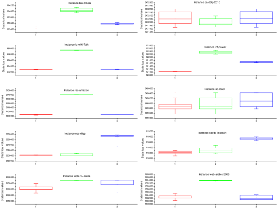
Figure 1: The dominate set values of massive graphs obtained by 1: CC²FS; 2: CC²FS+BREAK; 3: CCFS. Box plots are applied to display the distribution of these values.

8 Summary and Future Work

This paper presented a local search algorithm called CC²FS for solving the minimum weight dominating set (MWDS) problem. We proposed a new configuration checking strategy namely CC² based on the two-level neighborhood of vertices to remember the relevant information of removed and added vertices and prevent visiting the recent paths. Moreover, we introduced a new frequency based scoring function for solving MWDS. The experimental results showed that CC²FS performs essentially better than state of the art algorithms on almost all instances in terms of solution quality and run time.

As for future work, we consider to further improve the CC²FS algorithm by integrating some other ideas like strong configuration checking (?). Also we would like to test our algorithms on other instances including larger graphs. Envisioned research directions about the proposed strategies include applying the new score functions to other local search algorithms, and trying to find some other important properties and scoring functions of local search algorithms.

Acknowledgments

The authors of this paper wish to extend their sincere gratitude to all the anonymous reviewers for their efforts. Shaowei Cai is also supported by Youth Innovation Promotion Association, Chinese Academy of Sciences. For any theoretical and experimental problem arising from this paper, please correspondence to Professor Minghao Yin. This work was supported in part by NSFC (under Grant Nos. 61370156, 61503074, 61502464, 61402070, 61403077, and 61403076), China National 973 program 2014CB340301 and the Program for New Century Excellent Talents in University (NCET-13-0724).

References

- Abramé, Habet, & Toumi Abramé, A., Habet, D., & Toumi, D. (2014). Improving configuration checking for satisfiable random k-SAT instances. Annals of Mathematics and Artificial Intelligence, 1–20.
- Ahonen, de Alvarenga, & Amaral Ahonen, H., de Alvarenga, A. G., & Amaral, A. (2014). Simulated annealing and tabu search approaches for the corridor allocation problem. European Journal of Operational Research, 232(1), 221–233.
- Ambühl, Erlebach, Mihalák, & Nunkesser Ambühl, C., Erlebach, T., Mihalák, M., & Nunkesser, M. (2006). Constant-factor approximation for minimum-weight (connected) dominating sets in unit disk graphs. In Approximation, Randomization, and Combinatorial Optimization. Algorithms and Techniques, pp. 3–14. Springer.
- Aoun, Boutaba, Iraqi, & Kenward Aoun, B., Boutaba, R., Iraqi, Y., & Kenward, G. (2006). Gateway placement optimization in wireless mesh networks with QoS constraints. Selected Areas in Communications, IEEE Journal on, 24(11), 2127–2136.
- Bouamama & Blum Bouamama, S., & Blum, C. (2016). A hybrid algorithmic model for the minimum weight dominating set problem. Simulation Modelling Practice and Theory, 64, 57–68.
- Cai, Jie, & Su Cai, S., Jie, Z., & Su, K. (2015). An effective variable selection heuristic in SLS for weighted Max-2-SAT. Journal of Heuristics, 21(3), 433–456.
- Cai & Su Cai, S., & Su, K. (2012). Configuration checking with aspiration in local search for sat. In Proceedings of the Twenty-Sixth AAAI Conference on Artificial Intelligence, pp. 434–440. AAAI Press.
- Cai & Su Cai, S., & Su, K. (2013). Local search for boolean satisfiability with configuration checking and subscore. Artificial Intelligence, 204, 75–98.
- Cai, Su, Luo, & Sattar Cai, S., Su, K., Luo, C., & Sattar, A. (2013). NuMVC: An efficient local search algorithm for minimum vertex cover. Journal of Artificial Intelligence Research, 46, 687–716.
- Cai, Su, & Sattar Cai, S., Su, K., & Sattar, A. (2011). Local search with edge weighting and configuration checking heuristics for minimum vertex cover. Artificial Intelligence, 175(9), 1672–1696.
- Chaurasia & Singh Chaurasia, S. N., & Singh, A. (2015). A hybrid evolutionary algorithm with guided mutation for minimum weight dominating set. Applied Intelligence, 43(3), 512–529.
- Cockayne, Dawes, & Hedetniemi Cockayne, E. J., Dawes, R., & Hedetniemi, S. T. (1980). Total domination in graphs. Networks, 10(3), 211–219.
- Dai & Yu Dai, D., & Yu, C. (2009). A 5+-approximation algorithm for minimum weighted dominating set in unit disk graph. Theoretical Computer Science, 410(8), 756–765.
- Di Gaspero & Schaerf Di Gaspero, L., & Schaerf, A. (2007). A composite-neighborhood tabu search approach to the traveling tournament problem. Journal of Heuristics, 13(2), 189–207.
- El Houmaidi & Bassiouni El Houmaidi, M., & Bassiouni, M. A. (2003). k-weighted minimum dominating sets for sparse wavelength converters placement under nonuniform traffic. In Modeling, Analysis and Simulation of Computer Telecommunications Systems, 2003. MASCOTS 2003. 11th IEEE/ACM International Symposium on, pp. 56–61. IEEE.
- Escobar, Linfati, Toth, & Baldoquin Escobar, J. W., Linfati, R., Toth, P., & Baldoquin, M. G. (2014). A hybrid granular tabu search algorithm for the multi-depot vehicle routing problem. Journal of Heuristics, 20(5), 483–509.
- Fang, Chu, Qiao, Feng, & Xu Fang, Z., Chu, Y., Qiao, K., Feng, X., & Xu, K. (2014). Combining edge weight and vertex weight for minimum vertex cover problem. In International Workshop on Frontiers in Algorithmics, pp. 71–81. Springer.
- Gary & Johnson Gary, M. R., & Johnson, D. S. (1979). Computers and Intractability: A Guide to the Theory of NP-completeness. WH Freeman and Company, New York.
- Glover Glover, F. (1989). Tabu search-part i. ORSA Journal on computing, 1(3), 190–206.
- Houck, Joines, & Kay Houck, C. R., Joines, J. A., & Kay, M. G. (1996). Comparison of genetic algorithms, random restart and two-opt switching for solving large location-allocation problems. Computers & Operations Research, 23(6), 587–596.
- Johnson & Trick Johnson, D. S., & Trick, M. A. (1996). Cliques, coloring, and satisfiability: second DIMACS implementation challenge, October 11-13, 1993, Vol. 26. American Mathematical Soc.
- Jovanovic, Tuba, & Simian Jovanovic, R., Tuba, M., & Simian, D. (2010). Ant colony optimization applied to minimum weight dominating set problem. In Proceedings of the 12th WSEAS international conference on Automatic control, modelling & simulation, pp. 322–326. World Scientific and Engineering Academy and Society (WSEAS).
- Li & Huang Li, C. M., & Huang, W. Q. (2005). Diversification and determinism in local search for satisfiability. In International Conference on Theory and Applications of Satisfiability Testing, pp. 158–172. Springer.
- Li, Hu, Zhang, & Yin Li, R., Hu, S., Zhang, H., & Yin, M. (2016). An efficient local search framework for the minimum weighted vertex cover problem. Information Sciences, 372, 428–445.
- Luo, Cai, Su, & Wu Luo, C., Cai, S., Su, K., & Wu, W. (2015a). Clause states based configuration checking in local search for satisfiability. Cybernetics, IEEE Transactions on, 45(5), 1014–1027.
- Luo, Cai, Wu, Jie, & Su Luo, C., Cai, S., Wu, W., Jie, Z., & Su, K. (2015b). CCLS: An efficient local search algorithm for weighted maximum satisfiability. IEEE Trans. Computers, 64(7), 1830–1843.
- Michele Michele, M. (2007). The clustering simulation framework: a simple manual. http://www.michele-mastrogiovanni.net/software/download/README.pdf.
- Nitash & Singh Nitash, C., & Singh, A. (2014). An artificial bee colony algorithm for minimum weight dominating set. In Swarm Intelligence (SIS), 2014 IEEE Symposium on, pp. 1–7. IEEE.
- Polash, Newton, & Sattar Polash, M. A., Newton, M. H., & Sattar, A. (2015). Constraint-based local search for golomb rulers. In International Conference on AI and OR Techniques in Constriant Programming for Combinatorial Optimization Problems, pp. 322–331. Springer.
- Potluri & Singh Potluri, A., & Singh, A. (2013). Hybrid metaheuristic algorithms for minimum weight dominating set. Applied Soft Computing, 13(1), 76–88.
- Pullan Pullan, W. (2008). Approximating the maximum vertex/edge weighted clique using local search. Journal of Heuristics, 14(2), 117–134.
- Rossi & Ahmed Rossi, R., & Ahmed, N. (2015). The network data repository with interactive graph analytics and visualization. In Proceedings of the Twenty-Ninth AAAI Conference on Artificial Intelligence, pp. 4292–4293.
- Selman, Kautz, & Cohen Selman, B., Kautz, H. A., & Cohen, B. (1994). Noise strategies for improving local search. In Proceedings of the 12th National Conference on Artificial Intelligence, Vol. 94, pp. 337–343.
- Shen & Li Shen, C., & Li, T. (2010). Multi-document summarization via the minimum dominating set. In Proceedings of the 23rd International Conference on Computational Linguistics, pp. 984–992. Association for Computational Linguistics.
- Subhadrabandhu, Sarkar, & Anjum Subhadrabandhu, D., Sarkar, S., & Anjum, F. (2004). Efficacy of misuse detection in ad hoc networks. In Sensor and Ad Hoc Communications and Networks, 2004. IEEE SECON 2004. 2004 First Annual IEEE Communications Society Conference on, pp. 97–107. IEEE.
- Voudouris & Tsang Voudouris, C., & Tsang, E. P. (2003). Guided local search. In Handbook of metaheuristics, pp. 185–218. Springer.
- Wang, Cai, & Yin Wang, Y., Cai, S., & Yin, M. (2016). Two efficient local search algorithms for maximum weight clique problem. In Proceedings of the Thirtieth AAAI Conference on Artificial Intelligence, pp. 805–811.
- Wang, Ouyang, Zhang, & Yin Wang, Y., Ouyang, D., Zhang, L., & Yin, M. (2015). A novel local search for unicost set covering problem using hyperedge configuration checking and weight diversity. SCIENCE CHINA Information Sciences, 1–14.
- Wang, Yin, Ouyang, & Zhang Wang, Y., Yin, M., Ouyang, D., & Zhang, L. (2016). A novel local search algorithm with configuration checking and scoring mechanism for the set k-covering problem. International Transactions in Operational Research, 1–23.
- Wang, Wang, & Li Wang, Y., Wang, W., & Li, X.-Y. (2006). Efficient distributed low-cost backbone formation for wireless networks. Parallel and Distributed Systems, IEEE Transactions on, 17(7), 681–693.
- Wu, Wen, Liu, & Ma Wu, P., Wen, J.-R., Liu, H., & Ma, W.-Y. (2006). Query selection techniques for efficient crawling of structured web sources. In 22nd International Conference on Data Engineering (ICDE’06), pp. 47–47. IEEE.
- Xu, Boussemart, Hemery, & Lecoutre Xu, K., Boussemart, F., Hemery, F., & Lecoutre, C. (2005). A simple model to generate hard satisfiable instances. In Proceedings of the Nineteenth International Joint Conference on Artificial Intelligence, pp. 337–342.
- Xu, Boussemart, Hemery, & Lecoutre Xu, K., Boussemart, F., Hemery, F., & Lecoutre, C. (2007). Random constraint satisfaction: Easy generation of hard (satisfiable) instances. Artificial Intelligence, 171(8), 514–534.
- Xu & Li Xu, K., & Li, W. (2000). Exact phase transitions in random constraint satisfaction problems. Journal of Artificial Intelligence Research, 12(1), 93–103.
- Xu & Li Xu, K., & Li, W. (2006). Many hard examples in exact phase transitions. Theoretical Computer Science, 355(3), 291–302.
- Zhu, Wang, Shan, Wang, & Wu Zhu, X., Wang, W., Shan, S., Wang, Z., & Wu, W. (2012). A PTAS for the minimum weighted dominating set problem with smooth weights on unit disk graphs. Journal of combinatorial optimization, 23(4), 443–450.
- Zou, Wang, Xu, Li, Du, Wan, & Wu Zou, F., Wang, Y., Xu, X.-H., Li, X., Du, H., Wan, P., & Wu, W. (2011). New approximations for minimum-weighted dominating sets and minimum-weighted connected dominating sets on unit disk graphs. Theoretical Computer Science, 412(3), 198–208.