Analysis of the Linearized Problem of Quantitative Photoacoustic Tomography

Abstract

Quantitative image reconstruction in photoacoustic tomography requires the solution of a coupled physics inverse problem involving light transport and acoustic wave propagation. In this paper we address this issue employing the radiative transfer equation as accurate model for light transport. As main theoretical results, we derive several stability and uniqueness results for the linearized inverse problem. We consider the case of single illumination as well as the case of multiple illuminations assuming full or partial data. The numerical solution of the linearized problem is much less costly than the solution of the non-linear problem. We present numerical simulations supporting the stability results for the linearized problem and demonstrate that the linearized problem already gives accurate quantitative results.

Key words: Quantitative photoacoustic tomography, partial data, radiative transfer equation, multiple illuminations, linearization, two-sided stability estimates, image reconstruction.

AMS subject classification: 45Q05, 65R32, 47G30.

1 Introduction

Photoacoustic tomography (PAT) is a recently developed coupled physics imaging modality that combines the high spatial resolution of ultrasound imaging with the high contrast of optical imaging [14, 52, 79, 80, 83]. When a semitransparent sample is illuminated with a short pulse of laser light, parts of the optical energy are absorbed inside the sample, which in turn induces an acoustic pressure wave. In PAT, acoustic pressure waves are measured outside of the object of interest and mathematical algorithms are used to recover an image of the interior. Initial work and also recent works in PAT concentrated on the problem of reconstructing the initial pressure distribution, which has been considered as final diagnostic image (see, for example, [2, 17, 33, 34, 36, 35, 41, 43, 45, 48, 51, 54, 58, 55, 69, 71, 75, 83]). However, the initial pressure distribution only provides qualitative information about the tissue-relevant parameters. This is due to the fact that the initial pressure distribution is the product of the optical absorption coefficient and the spatially varying optical intensity which again indirectly depends on the tissue parameters. Quantitative photoacoustic tomography (qPAT) addresses this issue and aims at quantitatively estimating the tissue parameters by supplementing the inversion of the acoustic wave equation with an inverse problem for the light propagation (see, for example, [53, 22, 21, 72, 85, 3, 8, 11, 19, 23, 76, 70, 73, 61, 65, 25, 42]).

The radiative transfer equation (RTE) is commonly considered as a very accurate model for light transport in tissue (see, for example, see [4, 24, 30, 50]) and will be employed in this paper. As proposed in [42] we work with a single-stage reconstruction procedure for qPAT, where the optical parameters are reconstructed directly from the measured acoustical data. This is in contrast to the more common two-stage procedure, where the measured boundary pressure values are used to recover the initial internal pressure distribution in an intermediate step, and the spatially varying tissue parameters are estimated from the initial pressure distribution in a second step. However, as pointed out in [38, 42], the two-stage approach has several drawbacks, such as the missing capability of dealing with multiple illuminations using incomplete acoustic measurements in each experiment. The single-stage strategy can also be combined with the diffusion approximation; see [9, 16, 27, 38, 86]. The diffusion approximation is numerically less costly to solve than the RTE. However, we work with the RTE since it is the more accurate model for light propagation in tissue.

1.1 The linearized inverse problem of qPAT

In this paper, we study the linearized inverse problem of qPAT using the RTE. We present a uniqueness and stability analysis for both single and multiple illuminations. Our strategy is to first analyze the optical (heating) and acoustic processes separately, and then combine them together. The uniqueness and stability analysis of the acoustic process is well established and we make use of existing results. The study of the heating process, on the other hand, is much less understood. Its analysis is our main emphasis and our contribution includes several uniqueness and stability results. We derive stability estimates of the form

$$C_{1}\|h_{a}\|_{L^{2}(\Omega)}\leq\|\mathbf{W}\mathbf{D}h_{a}\|_{L^{2}(\Lambda\times(0,T))}\leq C_{2}\|h_{a}\|_{L^{2}(\Omega)}\,,$$

for the unknown absorption parameter perturbation $h_{a}=\mu_{a}-\mu_{a}^{\star}$, where $\mu_{a}$ and $\mu_{a}^{\star}$ are the actual and background absorption coefficients, respectively. Here $\mathbf{W}\mathbf{D}\colon L^{2}(\Omega)\to L^{2}(\Lambda\times(0,T))$ is the linearized forward operator of qPAT with respect to the attenuation at $\mu_{a}^{\star}$. Such results are derived under different conditions for vanishing scattering (Theorems 3.5 and 3.6), non-vanishing scattering (Theorem 3.8), as well as multiple illuminations (Theorem  3.9). Our analysis is inspired by [56] where microlocal analysis was employed to analyze the stability of an inverse problem with internal data (see also [7, 10, 13, 57, 64, 81] for related works). We also take advantage of previous works on RTE [74, 29] and microlocal acoustic wave inversion [75].

The feasibility of solving the linearized problem is illustrated by numerical simulations presented in Section 4. For numerically solving the linearized problem we use the Landweber iteration that can also be employed for the fully non-linear problem, see [42]. We point out that solving the linearized inverse problem is computationally much less costly than solving the fully non-linear problem. Our numerical results show that in many situation the solution of the linearized problem already gives quite accurate reconstruction results.

1.2 Outline

The rest of the paper is organized as follows. In Section 2 we present a Hilbert space framework for qPAT using the RTE. We consider the single illumination as well as the multiple illumination case and recall the well-posedness of the non-linear forward operator. We further give its Gâteaux-derivative, whose inversion constitutes the linearized inverse problem of qPAT. In Section 3 we present our main stability and uniqueness results for the linearized inverse problem. Our theoretical results are supplemented by numerical examples presented in Section 4. The paper concludes with a short summary and outlook presented in Section 5.

2 The forward problem in qPAT

In this section we describe the forward problem of qPAT in a Hilbert space framework using the RTE. Allowing for $N$ different illumination patterns, the forward problem is given by a nonlinear operator $\mathbf{F}=(\mathbf{W}_{i}\circ\mathbf{H}_{i})_{i=1}^{N}$, where the operator $\mathbf{H}_{i}$ models the optical heating and $\mathbf{W}_{i}$ the acoustic measurement due to the $i$-th illumination. These operators are described and analyzed in detail in the following.

2.1 Notation

Throughout this paper, $\Omega\subseteq\mathbb{R}^{d}$ denotes a convex bounded domain with Lipschitz-boundary $\partial\Omega$, where $d\geq 2$ denotes the spatial dimension. We write

$$\Gamma_{-} \coloneqq\left\{(x,\theta)\in\partial\Omega\times\mathbb{S}^{d-1}\mid{\nu(x)}\mathchoice{\mathbin{\vbox{\hbox{\scalebox{0.6}{$\displaystyle\bullet$}}}}}{\mathbin{\vbox{\hbox{\scalebox{0.6}{$\textstyle\bullet$}}}}}{\mathbin{\vbox{\hbox{\scalebox{0.6}{$\scriptstyle\bullet$}}}}}{\mathbin{\vbox{\hbox{\scalebox{0.6}{$\scriptscriptstyle\bullet$}}}}}{\theta}<0\right\}\,.$$

Here $\nu(x)$ denotes the outward unit normal at $x\in\partial\Omega$ and ${a}\mathchoice{\mathbin{\vbox{\hbox{\scalebox{0.6}{$\displaystyle\bullet$}}}}}{\mathbin{\vbox{\hbox{\scalebox{0.6}{$\textstyle\bullet$}}}}}{\mathbin{\vbox{\hbox{\scalebox{0.6}{$\scriptstyle\bullet$}}}}}{\mathbin{\vbox{\hbox{\scalebox{0.6}{$\scriptscriptstyle\bullet$}}}}}{b}$ the standard scalar product of $a,b\in\mathbb{R}^{d}$. We denote by $L^{2}(\Gamma_{-},\lvert{\nu}\mathchoice{\mathbin{\vbox{\hbox{\scalebox{0.6}{$\displaystyle\bullet$}}}}}{\mathbin{\vbox{\hbox{\scalebox{0.6}{$\textstyle\bullet$}}}}}{\mathbin{\vbox{\hbox{\scalebox{0.6}{$\scriptstyle\bullet$}}}}}{\mathbin{\vbox{\hbox{\scalebox{0.6}{$\scriptscriptstyle\bullet$}}}}}{\theta}\rvert)$ the space of all measurable functions $f$ defined on $\Gamma_{-}$ such that

$$\left\|f\right\|_{L^{2}(\Gamma_{-},\lvert{\nu}\mathchoice{\mathbin{\vbox{\hbox{\scalebox{0.6}{$\displaystyle\bullet$}}}}}{\mathbin{\vbox{\hbox{\scalebox{0.6}{$\textstyle\bullet$}}}}}{\mathbin{\vbox{\hbox{\scalebox{0.6}{$\scriptstyle\bullet$}}}}}{\mathbin{\vbox{\hbox{\scalebox{0.6}{$\scriptscriptstyle\bullet$}}}}}{\theta}\rvert)}\coloneqq\sqrt{\int_{\Gamma_{-}}\left|{\nu(x)}\mathchoice{\mathbin{\vbox{\hbox{\scalebox{0.6}{$\displaystyle\bullet$}}}}}{\mathbin{\vbox{\hbox{\scalebox{0.6}{$\textstyle\bullet$}}}}}{\mathbin{\vbox{\hbox{\scalebox{0.6}{$\scriptstyle\bullet$}}}}}{\mathbin{\vbox{\hbox{\scalebox{0.6}{$\scriptscriptstyle\bullet$}}}}}{\theta}\right|\left|f(x,\theta)\right|^{2}\mathrm{d}(x,\theta)}<\infty\,.$$ (2.1)

We further denote by $W^{2}(\Omega\times\mathbb{S}^{d-1})$ the space of all measurable functions defined on $\Omega\times\mathbb{S}^{d-1}$ such that

$$\left\|\Phi\right\|_{W^{2}(\Omega\times\mathbb{S}^{d-1})}^{2}\coloneqq\left\|\Phi\right\|_{L^{2}(\Omega\times\mathbb{S}^{d-1})}^{2}+\left\|{\theta}\mathchoice{\mathbin{\vbox{\hbox{\scalebox{0.6}{$\displaystyle\bullet$}}}}}{\mathbin{\vbox{\hbox{\scalebox{0.6}{$\textstyle\bullet$}}}}}{\mathbin{\vbox{\hbox{\scalebox{0.6}{$\scriptstyle\bullet$}}}}}{\mathbin{\vbox{\hbox{\scalebox{0.6}{$\scriptscriptstyle\bullet$}}}}}{\nabla_{x}\Phi}\right\|_{L^{2}(\Omega\times\mathbb{S}^{d-1})}^{p}+\left\|\Phi|_{\Gamma_{-}}\right\|_{L^{2}\left(\Gamma_{-},\left|{\nu}\mathchoice{\mathbin{\vbox{\hbox{\scalebox{0.6}{$\displaystyle\bullet$}}}}}{\mathbin{\vbox{\hbox{\scalebox{0.6}{$\textstyle\bullet$}}}}}{\mathbin{\vbox{\hbox{\scalebox{0.6}{$\scriptstyle\bullet$}}}}}{\mathbin{\vbox{\hbox{\scalebox{0.6}{$\scriptscriptstyle\bullet$}}}}}{\theta}\right|\right)}^{2}$$ (2.2)

is well defined and finite. The subspace of all elements $\Phi\in W^{2}(\Omega\times\mathbb{S}^{d-1})$ satisfying $\Phi|_{\Gamma_{-}}=0$ will be denoted by $W^{2}_{0}(\Omega\times\mathbb{S}^{d-1})$. The spaces $L^{\infty}(\Gamma_{-},\lvert{\nu}\mathchoice{\mathbin{\vbox{\hbox{\scalebox{0.6}{$\displaystyle\bullet$}}}}}{\mathbin{\vbox{\hbox{\scalebox{0.6}{$\textstyle\bullet$}}}}}{\mathbin{\vbox{\hbox{\scalebox{0.6}{$\scriptstyle\bullet$}}}}}{\mathbin{\vbox{\hbox{\scalebox{0.6}{$\scriptscriptstyle\bullet$}}}}}{\theta}\rvert)$, $W^{\infty}(\Omega\times\mathbb{S}^{d-1})$ and $W^{\infty}_{0}(\Omega\times\mathbb{S}^{d-1})$ are defined in a similar manner by considering the $L^{\infty}$-norms instead of the $L^{2}$-norms in (2.1), (2.2).

For fixed positive numbers $\bar{\mu}_{a},\bar{\mu}_{s}>0$ we write

$$\mathcal{M}\coloneqq\bigl{\{}(\mu_{a},\mu_{s})\in L^{2}\left(\Omega\right)\times L^{2}(\Omega)\mid 0\leq\mu_{s}\leq\bar{\mu}_{s}\text{ and }0\leq\mu_{a}\leq\bar{\mu}_{a}\bigr{\}}\,,$$ (2.3)

for the parameter set of unknown attenuation and scattering coefficients. Note that $\mathcal{M}$ is a closed, bounded and convex subset of $L^{2}\left(\Omega\right)\times L^{2}\left(\Omega\right)$ with empty interior. Finally, we denote by $C^{\infty}_{\Omega}(\mathbb{R}^{d})$ and $L^{p}_{\Omega}(\mathbb{R}^{d})$, for $p\in[1,\infty]$, the set of all elements in $C^{\infty}(\mathbb{R}^{d})$ and $L^{p}(\mathbb{R}^{d})$ that vanish outside of $\Omega$.

2.2 The heating operator

Throughout this subsection, let $q\in L^{\infty}(\Omega\times\mathbb{S}^{d-1})$ and $f\in L^{\infty}\left(\Gamma_{-},\left|{\nu}\mathchoice{\mathbin{\vbox{\hbox{\scalebox{0.6}{$\displaystyle\bullet$}}}}}{\mathbin{\vbox{\hbox{\scalebox{0.6}{$\textstyle\bullet$}}}}}{\mathbin{\vbox{\hbox{\scalebox{0.6}{$\scriptstyle\bullet$}}}}}{\mathbin{\vbox{\hbox{\scalebox{0.6}{$\scriptscriptstyle\bullet$}}}}}{\theta}\right|\right)$ be a given source pattern and boundary light source, respectively. Further, we denote by $k\colon\mathbb{S}^{d-1}\times\mathbb{S}^{d-1}\to\mathbb{R}$ the scattering kernel, which is supposed to be a symmetric and nonnegative function that satisfies $\int_{\mathbb{S}^{d-1}}k\left(\,\cdot\,,\theta^{\prime}\right)\mathrm{d}\theta^{\prime}=1$.

We model the optical radiation by a function $\Phi\colon\Omega\times\mathbb{S}^{d-1}\to\mathbb{R}$, where $\Phi\left(x,\theta\right)$ is the density of photons at location $x\in\Omega$ propagating in direction $\theta\in\mathbb{S}^{d-1}$. The photon density is supposed to satisfy the RTE,

$$\left\{\begin{aligned} \left({\theta}\mathchoice{\mathbin{\vbox{\hbox{\scalebox{0.6}{$\displaystyle\bullet$}}}}}{\mathbin{\vbox{\hbox{\scalebox{0.6}{$\textstyle\bullet$}}}}}{\mathbin{\vbox{\hbox{\scalebox{0.6}{$\scriptstyle\bullet$}}}}}{\mathbin{\vbox{\hbox{\scalebox{0.6}{$\scriptscriptstyle\bullet$}}}}}{\nabla_{x}}+\left(\mu_{a}+\mu_{s}-\mu_{s}\mathbf{K}\right)\right)\Phi&=q&&\text{ in }\Omega\times\mathbb{S}^{d-1}\\ \Phi|_{\Gamma_{-}}&=f&&\text{ on }\Gamma_{-}\,.\end{aligned}\right.$$ (2.4)

Here $\mathbf{K}\colon L^{2}(\Omega\times\mathbb{S}^{d-1})\to L^{2}(\Omega\times\mathbb{S}^{d-1})$ denotes the scattering operator defined by $\left(\mathbf{K}\Phi\right)\left(x,\theta\right)=\int_{\mathbb{S}^{d-1}}k(\theta,\theta^{\prime})\Phi(x,\theta^{\prime})\mathrm{d}\theta^{\prime}$. See, for example, [6, 28, 30, 62, 74] for the RTE in optical tomography.

Lemma 2.1 (Well-posedness of the RTE).

For every $(\mu_{a},\mu_{s})\in\mathcal{M}$, (2.4) admits a unique solution $\Phi\in W^{2}(\Omega\times\mathbb{S}^{d-1})$. Moreover, there exists a constant $C_{2}(\bar{\mu}_{a},\bar{\mu}_{s})$ only depending on $\bar{\mu}_{a}$ and $\bar{\mu}_{s}$, such that the following a-priori estimate holds

$$\left\|\Phi\right\|_{W^{2}(\Omega\times\mathbb{S}^{d-1})}\leq C_{2}(\bar{\mu}_{a},\bar{\mu}_{s})\left(\left\|q\right\|_{L^{2}(\Omega\times\mathbb{S}^{d-1})}+\left\|f\right\|_{L^{2}\left(\Gamma_{-},\left|{\nu}\mathchoice{\mathbin{\vbox{\hbox{\scalebox{0.6}{$\displaystyle\bullet$}}}}}{\mathbin{\vbox{\hbox{\scalebox{0.6}{$\textstyle\bullet$}}}}}{\mathbin{\vbox{\hbox{\scalebox{0.6}{$\scriptstyle\bullet$}}}}}{\mathbin{\vbox{\hbox{\scalebox{0.6}{$\scriptscriptstyle\bullet$}}}}}{\theta}\right|\right)}\right)\,.$$ (2.5)

Proof.

See [29]. ∎

The absorption of photons causes a non-uniform heating of the tissue that is proportional to the total amount of absorbed photons. We model this by the heating operator $\mathbf{H}_{f,q}\colon\mathcal{M}\to L^{2}(\Omega)$ that is defined by

$$\mathbf{H}_{f,q}\left(\mu_{a},\mu_{s}\right)(x)\coloneqq\mu_{a}(x)\int_{\mathbb{S}^{d-1}}\Phi(x,\theta)\mathrm{d}\theta\quad\text{ for }x\in\Omega\,,$$ (2.6)

with $\Phi$ denoting the solution of (2.4).

Lemma 2.2.

The heating operator $\mathbf{H}_{f,q}\colon\mathcal{M}\to L^{2}(\Omega)$ is well defined, Lipschitz-continuous and weakly continuous.

Proof.

See [42]. ∎

We next compute the derivative of $\mathbf{H}_{f,q}$. For that purpose we call $h\in L^{2}(\Omega)\times L^{2}(\Omega)$ a feasible direction at $\mu=(\mu_{a},\mu_{s})\in\mathcal{M}$ if there exists some $\epsilon>0$ such that $\mu+\epsilon h\in\mathcal{M}$. The set of all feasible directions at $\mu$ will be denotes by $\mathcal{M}(\mu)$. For $\mu\in\mathcal{M}$ and $h\in\mathcal{M}(\mu)$ we denote the one-sided directional derivative of $\mathbf{H}_{f,q}$ at $\mu$ in direction $h$ by $\mathbf{H}_{f,q}^{\prime}(\mu)(h)$. If $\mathbf{H}_{f,q}^{\prime}(\mu)(h)$ and $-\mathbf{H}_{f,q}^{\prime}(\mu)(-h)$ exist and coincide on a dense subset of directions and $h\mapsto\mathbf{H}_{f,q}^{\prime}(\mu)(h)$ is bounded and linear, we say that $\mathbf{H}$ is Gâtaux differentiable at $\mu$ and call $\mathbf{H}_{f,q}^{\prime}(\mu)$ the Gâtaux derivative of $\mathbf{H}_{f,q}$ at $\mu$.

Lemma 2.3 (Differentiability of $\mathbf{H}_{f,q}$).

Suppose $\mu=(\mu_{a},\mu_{s})\in\mathcal{M}$.

1. The one-sided directional derivative of $\mathbf{H}_{f,q}$ at $\mu$ in any feasible direction $h=(h_{a},h_{s})\in\mathcal{M}(\mu)$ exists and is given by

   $$\mathbf{H}_{f,q}^{\prime}(\mu)(h)=h_{a}\int_{\mathbb{S}^{d-1}}\Phi(\,\cdot\,,\theta)\mathrm{d}\theta-\mu_{a}\int_{\mathbb{S}^{d-1}}\Psi(\,\cdot\,,\theta)\mathrm{d}\theta\,.$$ (2.7)

   Here $\Phi$ is the solution of (2.4) and $\Psi$ satisfies the RTE

   $$\left\{\begin{aligned} \left({\theta}\mathchoice{\mathbin{\vbox{\hbox{\scalebox{0.6}{$\displaystyle\bullet$}}}}}{\mathbin{\vbox{\hbox{\scalebox{0.6}{$\textstyle\bullet$}}}}}{\mathbin{\vbox{\hbox{\scalebox{0.6}{$\scriptstyle\bullet$}}}}}{\mathbin{\vbox{\hbox{\scalebox{0.6}{$\scriptscriptstyle\bullet$}}}}}{\nabla_{x}}+\mu_{a}+\mu_{s}-\mu_{s}\mathbf{K}\right)\Psi&=\left(h_{a}+h_{s}-h_{s}\mathbf{K}\right)\Phi&&\text{in }\Omega\times\mathbb{S}^{d-1}\\ \Psi|_{\Gamma_{-}}&=0&&\text{on }\Gamma_{-}\,.\end{aligned}\right.$$ (2.8)

2. If $\mu_{a},\mu_{s}>0$, then $\mathbf{H}_{f,q}$ is Gâteaux differentiable at $(\mu_{a},\mu_{s})$.

Proof.

See [42]. ∎

2.3 The wave equation

The optical heating induces an acoustic pressure wave $p\colon\mathbb{R}^{d}\times\left(0,\infty\right)\to\mathbb{R}$, which satisfies the initial value problem

$$\left\{\begin{aligned} \partial_{t}^{2}p(x,t)-\Delta p(x,t)&=0\,,&&\text{ for }\left(x,t\right)\in\mathbb{R}^{d}\times\left(0,\infty\right)\\ p\left(x,0\right)&=h(x)\,,&&\text{ for }x\in\mathbb{R}^{d}\\ \partial_{t}p\left(x,0\right)&=0\,,&&\text{ for }x\in\mathbb{R}^{d}\,.\end{aligned}\right.$$ (2.9)

For the sake of simplicity in (2.9) and below we assume the speed of sound to be constant and rescaled to one. Further, the initial data $h$ is assumed to be supported in $\Omega$.

We suppose that the acoustic measurements are made on a subset $\Lambda\subseteq\partial D$, where $D\subseteq\mathbb{R}^{d}$ is a bounded domain with smooth boundary such that $D\supseteq\bar{\Omega}$. The acoustic forward operator corresponding to the measurement set $\Lambda$ is defined by

$$\mathbf{W}_{\Lambda,T}\colon C_{\Omega}(\mathbb{R}^{d})\subseteq L^{2}_{\Omega}(\mathbb{R}^{d})\to L^{2}(\Lambda\times(0,T))\colon h\mapsto p|_{\Lambda\times(0,T)}\,,$$ (2.10)

where $p\colon\mathbb{R}^{d}\times(0,T)\to\mathbb{R}$ denotes the unique solution of (2.9).

Lemma 2.4.

$\mathbf{W}_{\Lambda,T}$ is well defined and bounded and therefore can be uniquely extended to a bounded linear operator $\mathbf{W}_{\Lambda,T}\colon L^{2}_{\Omega}(\mathbb{R}^{d})\to L^{2}\left(\Lambda\times(0,T)\right)$.

Proof.

See for example [42]. ∎

The operator $\mathbf{W}_{\Lambda,T}$ can be evaluated by well-known solution formulas (see, for example, [32, 49]). In two spatial dimensions a solution is given by

$$\left(\mathbf{W}_{\Lambda,T}h\right)\left(y,t\right)=\frac{1}{2\pi}\frac{\partial}{\partial t}\int_{0}^{t}\int_{\mathbb{S}^{1}}h(y+t\omega)\frac{r}{\sqrt{t^{2}-r^{2}}}\,\mathrm{d}\omega\,\mathrm{d}r\,,$$ (2.11)

Because $\mathbf{W}_{\Lambda,T}$ is bounded and linear, the adjoint $\mathbf{W}_{\Lambda,T}^{\ast}\colon L^{2}\left(\Lambda\times(0,T)\right)\to L^{2}_{\Omega}(\mathbb{R}^{d})$ is again well defined and bounded. Explicit expressions of $\mathbf{W}_{\Lambda,T}^{\ast}$ are easily deduced from explicit expression for the solution of the wave equation. For example, in two spatial dimensions we have

$$\left(\mathbf{W}_{\Lambda,T}^{*}v\right)\left(x\right)=-\frac{1}{2\pi}\int_{\Lambda}\int_{\lvert x-y\rvert}^{T}\frac{\partial_{t}v\left(y,t\right)}{\sqrt{t^{2}-\lvert x-y\rvert^{2}}}\,\mathrm{d}t\,\mathrm{d}S(y)\,,$$ (2.12)

for every $v\in C_{c}^{1}(\Lambda\times(0,T))$.

2.4 The forward operator in qPAT

As being common in qPAT, we are interested in the case of a single illumination as well as multiple illuminations. Suppose that $q_{i}\in L^{\infty}(\Omega\times\mathbb{S}^{d-1})$ and $f_{i}\in L^{\infty}\left(\Gamma_{-},\lvert{\nu}\mathchoice{\mathbin{\vbox{\hbox{\scalebox{0.6}{$\displaystyle\bullet$}}}}}{\mathbin{\vbox{\hbox{\scalebox{0.6}{$\textstyle\bullet$}}}}}{\mathbin{\vbox{\hbox{\scalebox{0.6}{$\scriptstyle\bullet$}}}}}{\mathbin{\vbox{\hbox{\scalebox{0.6}{$\scriptscriptstyle\bullet$}}}}}{\theta}\rvert\right)$, for $i=1,\dots,N$, denote given source patterns and boundary light sources, respectively, where $N$ is the number of different illumination patterns. The case $N=1$ corresponds to a single illumination. We further denote by $\Lambda_{i}$ the surface where the acoustic measurements for the $i$-th illumination are made and $T_{i}$ the measurement duration. Let us mention that multiple illuminations are often implemented in PAT (see, e.g., [31] for such an experimental setup). Single-stage qPAT with multiple illuminations has been studied in [27, 38, 42, 9, 60]. Moreover, multiple illuminations have been proposed in several mathematical works to stabilize various inverse problems with internal data (e.g., [12, 11, 7, 10, 13, 57, 64, 81]).

For each illumination and measurement, we denote by $\mathbf{H}_{i}\coloneqq\mathbf{H}_{f_{i},q_{i}}$ and $\mathbf{W}_{i}\coloneqq\mathbf{W}_{\Lambda_{i},T}$ the corresponding heating and acoustic operator and by $\mathbf{F}_{i}=\mathbf{W}_{i}\circ\mathbf{H}_{i}$ the resulting forward operator. The total forward operator in qPAT allowing multiple illuminations is then given by

$$\mathbf{F}=(\mathbf{F}_{i})_{i=1}^{N}\colon\mathcal{M}\to\left(L^{2}(\Lambda\times(0,T))\right)^{N}$$ (2.13)

From Lemmas 2.2 and 2.4 it follows that the forward operator $\mathbf{F}$ is well defined, Lipschitz-continuous and weakly continuous.

Lemma 2.5 (Differentiability of $\mathbf{F}$).

Let $\mu=(\mu_{a},\mu_{s})\in\mathcal{M}$.

1. The one-sided directional derivative of $\mathbf{F}$ at $\mu$ in any feasible direction $h=(h_{a},h_{s})\in\mathcal{M}(\mu)$ exists and, with $\mathbf{H}_{i}^{\prime}$ as in Proposition 2.3, is given by

   $$\mathbf{F}^{\prime}(\mu)=(\mathbf{W}_{i}\circ\mathbf{H}_{i}^{\prime}(\mu))_{i=1}^{N}\,.$$ (2.14)

2. If $\mu_{a},\mu_{s}>0$, then $\mathbf{F}$ is Gâteaux differentiable at $\mu$.

Proof.

Follows from Proposition 2.3 and Lemma 2.4. ∎

The derivative $\mathbf{F}^{\prime}(\mu)$ is the linearized forward operator in qPAT that we will analyze in the following.

3 Analysis of the linearized inverse problem

In this section we study uniqueness and stability of the problem of inverting $\mathbf{F}^{\prime}(\mu_{a},\mu_{s})$, where $(\mu_{a}^{\star},\mu_{s}^{\star})\in\mathcal{M}$ is a fixed pair of background optical absorption and scattering coefficients.

We denote by $\mathbf{V}\colon W^{\infty}(\Omega\times\mathbb{S}^{d-1})\to L^{\infty}(\Omega\times\mathbb{S}^{d-1})$ the transport operator defined by $\mathbf{V}\Phi\coloneqq\left({\theta}\mathchoice{\mathbin{\vbox{\hbox{\scalebox{0.6}{$\displaystyle\bullet$}}}}}{\mathbin{\vbox{\hbox{\scalebox{0.6}{$\textstyle\bullet$}}}}}{\mathbin{\vbox{\hbox{\scalebox{0.6}{$\scriptstyle\bullet$}}}}}{\mathbin{\vbox{\hbox{\scalebox{0.6}{$\scriptscriptstyle\bullet$}}}}}{\nabla_{x}}+\mu_{a}\right)\Phi$ and write $\mathbf{V}_{0}$ for the restriction to $W^{\infty}_{0}(\Omega\times\mathbb{S}^{d-1})$. Then, $\mathbf{V}_{0}$ is invertible and its inverse is given by

$$(\mathbf{V}_{0}^{-1}\Psi)(x,\theta)=\int_{0}^{\ell(x,\theta)}e^{-\int_{0}^{t}\mu_{a}(x-\tau\theta)\,\mathrm{d}\tau}\,\Psi(x-t\theta,\theta)\,\mathrm{d}t\,.$$ (3.1)

Here, $\ell(x,\theta)$ is the supremum over all $s>0$ such that $x-s\theta\in\Omega$. That is, $\ell(x,\theta)$ is the distance from $x$ to the boundary $\partial\Omega$ along the direction $-\theta$. It is easy to see that $\mathbf{V}_{0}^{-1}$ is a bounded operator when considered as mapping from $L^{\infty}(\Omega\times\mathbb{S}^{d-1})$ into itself and satisfies

$$\|\mathbf{V}_{0}^{-1}\|_{L^{\infty},L^{\infty}}\leq\operatorname{diam}(\Omega)\,.$$ (3.2)

3.1 An auxiliary result

The following result plays a key role in our subsequent analysis.

Lemma 3.1.

Suppose $a\in C^{\infty}(\Omega\times\mathbb{S}^{d-1}\times[0,\infty))$ is compactly supported with respect to the last variable $t$. For each $q\in C_{c}^{\infty}(\Omega)$, we define

$$P(q)(x)\coloneqq\int_{0}^{\infty}\int_{\mathbb{S}^{d-1}}a(x,\theta,t)\,q(x-t\theta)\mathrm{d}\theta\,\mathrm{d}t$$

Then, $P$ extends to a pseudodifferential operator of order at most $-1/2$ on $\Omega$.

Proof.

We have $q(x-t\theta)=(2\pi)^{-d}\int_{\mathbb{R}^{d}}\int_{\mathbb{R}^{d}}e^{\mathsf{i}\left<x-t\theta-y,\xi\right>}q(y)\,\mathrm{d}y\,\mathrm{d}\xi$. Therefore,

$$P(q)(x) =\int_{0}^{\infty}\int_{\mathbb{S}^{d-1}}a(x,\theta,t)\,q(x-t\theta)\mathrm{d}\theta\,\mathrm{d}t$$

$$=\frac{1}{(2\pi)^{d}}\int_{0}^{\infty}\int_{\mathbb{S}^{d-1}}a(x,\theta,t)\,\int_{\mathbb{R}^{d}}\int_{\mathbb{R}^{d}}e^{\mathsf{i}\left<x-t\theta-y,\xi\right>}q(y)\,\mathrm{d}y\,\mathrm{d}\xi\mathrm{d}\theta\,\mathrm{d}t$$

$$=\frac{1}{(2\pi)^{d}}\int_{\mathbb{R}^{d}}\int_{\mathbb{R}^{d}}b(x,\xi)e^{\mathsf{i}\left<x-y,\xi\right>}q(y)\,\mathrm{d}y\,\mathrm{d}\xi\,,$$

where $b(x,\xi)\coloneqq\int_{\mathbb{S}^{d-1}}\int_{0}^{\infty}a(x,\theta,t)e^{-\mathsf{i}t\langle\theta,\xi\rangle}\,\mathrm{d}t\,\mathrm{d}\theta\,.$

We prove that $(x,\xi)\mapsto b(x,\xi)$ is a symbol of order at most $-1/2$. For that purpose, let $0\leq\chi\in C^{\infty}_{0}(\mathbb{R})\leq 1$ be a cut-off function that is equal to $1$ on $[-1,1]$ and zero outside of $[-2,2]$. Then

$$b(x,\xi)=\int_{\mathbb{S}^{d-1}}\int_{0}^{\infty}\left(1-\chi\Big{(}\frac{\langle\xi,\theta\rangle}{\lvert\xi\rvert^{1/2}}\Big{)}\right)\,a(x,\theta,t)e^{-\mathsf{i}t\langle\theta,\xi\rangle}\,\mathrm{d}t\,\mathrm{d}\theta\\ +\int_{\mathbb{S}^{d-1}}\int_{0}^{\infty}\chi\Big{(}\frac{\langle\xi,\theta\rangle}{\lvert\xi\rvert^{1/2}}\Big{)}\,a(x,\theta,t)e^{-\mathsf{i}t\langle\theta,\xi\rangle}\,\mathrm{d}t\,\mathrm{d}\theta=:I_{1}(x,\xi)+I_{2}(x,\xi).$$ (3.3)

To estimate $I_{1}(x,\xi)$, we write

$$I_{1}(x,\xi) =\int_{\mathbb{S}^{d-1}}\int_{0}^{\infty}\left(1-\chi\left(\frac{\langle\xi,\theta\rangle}{\lvert\xi\rvert^{1/2}}\right)\right)\,a(x,\theta,t)e^{-\mathsf{i}t\langle\theta,\xi\rangle}\,\mathrm{d}t\,\mathrm{d}\theta$$

$$=\int_{\mathbb{S}^{d-1}}\left(1-\chi\left(\frac{\langle\xi,\theta\rangle}{\lvert\xi\rvert^{1/2}}\right)\right)\,\frac{1}{\mathsf{i}\langle\theta,\xi\rangle}\Bigl{[}a(x,\theta,0)+\int_{0}^{\infty}a^{\prime}(x,\theta,t)e^{-\mathsf{i}t\langle\theta,\xi\rangle}\,\mathrm{d}t\Bigr{]}\,\mathrm{d}\theta$$

$$=\int_{\mathbb{S}^{d-1},|\langle\xi,\theta\rangle|\geq\lvert\xi\rvert^{1/2}}\frac{1-\chi\bigl{(}\frac{\langle\xi,\theta\rangle}{\lvert\xi\rvert^{1/2}}\bigr{)}}{\mathsf{i}\langle\theta,\xi\rangle}\Bigl{[}a(x,\theta,0)+\int_{0}^{\infty}a^{\prime}(x,\theta,t)e^{-\mathsf{i}t\langle\theta,\xi\rangle}\,\mathrm{d}t\Bigr{]}\,\mathrm{d}\theta\,,$$

and therefore $\left|I_{1}(x,\xi)\right|\leq C\lvert\xi\rvert^{-1/2}$ for $\lvert\xi\rvert\geq 1$. To estimate $I_{2}(x,\xi)$, note that the set $\{\theta\in\mathbb{S}^{d-1}\mid\lvert\langle\xi,\theta\rangle\rvert\leq 2\lvert\xi\rvert^{1/2}\}$ has measure proportional to $\lvert\xi\rvert^{-1/2}$ which shows

$$\left|I_{2}(x,\xi)\right|=\Bigl{|}\int_{\mathbb{S}^{d-1}}\int_{0}^{\infty}\chi\left(\frac{\langle\xi,\theta\rangle}{\lvert\xi\rvert^{1/2}}\right)\,a(x,\theta,t)e^{-\mathsf{i}t\langle\theta,\xi\rangle}\,\mathrm{d}t\,\mathrm{d}\theta\Bigr{|}\leq C\,\lvert\xi\rvert^{-\frac{1}{2}}\;\text{ for }\lvert\xi\rvert\geq 1\,.$$

Together with (3.3), we obtain $|b(x,\xi)|\leq C\lvert\xi\rvert^{-\frac{1}{2}}$ for $\lvert\xi\rvert\geq 1$.

Next we estimate $\partial_{\xi_{j}}b(x,\xi)=-\mathsf{i}\,\int_{\mathbb{S}^{d-1}}\int_{0}^{\infty}[t\theta_{j}a(x,\theta,t)]e^{-\mathsf{i}t\langle\theta,\xi\rangle}\,\mathrm{d}t\,\mathrm{d}\theta$. We consider the case $d=2$ only, the proof for general dimension follows in a similar manner. Let us write $\theta=(\cos(\phi),\sin(\phi))$. Then, using the expression of the gradient operator in polar coordinates, we obtain

$$\biggl{[}\xi_{1}\left(\cos(\phi)\partial_{t}-\frac{\sin(\phi)}{t}\partial_{\phi}\right)+\xi_{2}\left(\sin(\phi)\partial_{t}+\frac{\cos(\phi)}{t}\partial_{\phi}\right)\biggr{]}\,e^{-\mathsf{i}t\langle\theta,\xi\rangle}=-\mathsf{i}\,\lvert\xi\rvert^{2}\,e^{-\mathsf{i}t\langle\theta,\xi\rangle}$$

Together with one integration by parts this shows

$$\partial_{\xi_{j}}b(x,\xi) =\frac{1}{\lvert\xi\rvert^{2}}\,\int_{\mathbb{S}^{d-1}}\int_{0}^{\infty}t\theta_{j}a(x,\theta,t)\,\biggl{[}\xi_{1}\left(\cos(\phi)\partial_{t}-\frac{\sin(\phi)}{t}\partial_{\phi}\right)$$

$$\hskip 108.405pt+\xi_{2}\left(\sin(\phi)\partial_{t}+\frac{\cos(\phi)}{t}\partial_{\phi}\right)\biggr{]}\,e^{-\mathsf{i}t\langle\theta,\xi\rangle}\,\mathrm{d}t\,\mathrm{d}\theta$$

$$=-\frac{1}{\lvert\xi\rvert^{2}}\,\int_{\mathbb{S}^{d-1}}\int_{0}^{\infty}e^{-\mathsf{i}t\langle\theta,\xi\rangle}\biggl{[}\xi_{1}\left(\cos(\phi)\partial_{t}-\frac{\sin(\phi)}{t}\partial_{\phi}\right)$$

$$\hskip 86.72267pt+\xi_{2}\left(\sin(\phi)\partial_{t}+\frac{\cos(\phi)}{t}\partial_{\phi}\right)\biggr{]}\,\left(t\theta_{j}a(x,\theta,t)\right)\,\mathrm{d}t\,\mathrm{d}\theta\,.$$

Using that the functions $(\cos(\phi)\partial_{t}-\sin(\phi)t^{-1}\partial_{\phi})(t\theta_{j}a)$, $(\sin(\phi)\partial_{t}+\cos(\phi)t^{-1}\partial_{\phi})(t\theta_{j}a)$ are contained $C^{\infty}(\Omega\times\mathbb{S}^{d-1}\times[0,\infty))$ and repeating the argument above, we conclude that $\lvert\partial_{\xi_{j}}b(x,\xi)\rvert\leq C\lvert\xi\rvert^{-3/2}$. Finally, in a similar manner one verifies $\lvert\partial^{\beta}_{x}\partial^{\alpha}_{\xi}b(x,\xi)\rvert\leq C_{\alpha,\beta}\lvert\xi\rvert^{-1/2+|\alpha|}$ for all $\alpha,\beta\in\mathbb{N}^{d}$, which concludes the proof. ∎

3.2 Vanishing scattering

In this subsection we assume zero scattering, and consider a single illumination $N=1$. For given $\mu_{a}>0$ we write $\mathbf{D}=\mathbf{H}^{\prime}(\mu_{a},0)( \,\cdot\,,0)$ for the linearized partial forward operator. It is given by (see Proposition 2.3)

$$\mathbf{D}(h_{a})(x)=h_{a}(x)\int_{\mathbb{S}^{d-1}}\Phi(x,\theta)\mathrm{d}\,\theta-\mu_{a}(x)\,\int_{\mathbb{S}^{d-1}}\Psi(x,\theta)\mathrm{d}\theta\,,$$ (3.4)

where $\Phi$ and $\Psi$ satisfy the following background and linearized problem

$$\mathbf{V}\Phi=q \text{such that }\Phi|_{\Gamma_{-}}=f\,,$$ (3.5)

$$\mathbf{V}\Psi=\mathbf{V}_{0}\Psi=h_{a}\Phi \text{such that }\Psi|_{\Gamma_{-}}=0\,,$$ (3.6)

respectively. According to (3.1), the solution of (3.6) equals

$$\Psi(x,\theta)=\mathbf{V}_{0}^{-1}(h_{a}\Phi)(x,\theta)=\int_{0}^{\ell(x,\theta)}(h_{a}\Phi)(x-t\theta,\theta)e^{-\int_{0}^{t}\mu_{a}(x-\tau\theta)\mathrm{d}\tau}\mathrm{d}t\,.$$ (3.7)

For notational conveniences, we denote by $\phi\coloneqq\int_{\mathbb{S}^{d-1}}\Phi(\,\cdot\,,\theta)\,\mathrm{d}\theta$ the background fluence. Further, let us fix a domain $\Omega_{0}\Subset\Omega$. We will always assume that $\mbox{supp}(h_{a})\subseteq\Omega_{0}$.

We will also study the linearized forward operator $\mathbf{F}^{\prime}(\mu_{a},0)(\,\cdot\,,0)=\mathbf{W}\mathbf{D}$, where $\mathbf{W}=\mathbf{W}_{\Lambda,T}$ is the solution operator of the wave equation for the measurement set $\Lambda\subseteq\partial D$ and measurement time $T>0$; see Subsection 2.3. For that purpose we recall the visibility condition A.2 for the wave inversion problem, which states that any line through $x\in\Omega$ intersects $\Lambda$ at a point of distance less than $T$ from $x$.

Lemma 3.2.

If $\Phi\in C^{\infty}(\overline{\Omega}\times\mathbb{S}^{d-1})$, then $h_{a}\to\int_{\mathbb{S}^{d-1}}\Psi(\,\cdot\,,\theta)\mathrm{d}\theta$ is a pseudo-differential operator of order at most $-1/2$ on $\Omega_{0}$.

Proof.

Let $\varphi\in C_{0}^{\infty}(\Omega)$ be such that $\varphi=1$ in $\Omega_{0}$. Then $h\varphi=h$, and according to (3.7) we have

$$\int_{\mathbb{S}^{d-1}}\Psi(x,\theta)\,\mathrm{d}\theta=\int_{0}^{\infty}\int_{\mathbb{S}^{d-1}}a(x,\theta,t)\,h_{a}(x-t\theta)\mathrm{d}t\,\mathrm{d}\theta,$$

with $a(x,\theta,t)\coloneqq\varphi(x-t\theta)\,\Phi(x-t\theta,\theta)\,e^{-\int_{0}^{t}\mu_{a}(x-\tau\theta)\mathrm{d}\tau}$. Together with Proposition 3.1 this implies that $h_{a}\to\int_{\mathbb{S}^{d-1}}\Psi(\,\cdot\,,\theta)\,\mathrm{d}\theta$ is a pseudo-differential operator of order at most $-1/2$ and concludes the proof. ∎

Lemma 3.2 in particular implies that $h_{a}\to\int_{\mathbb{S}^{d-1}}\Psi(x,\theta)\mathrm{d}\theta$ is boundedly maps $L^{2}(\Omega)$ to the Sobolev space $H^{1/2}(\Omega)$. Such weaker result also follows from the averaging lemma, which states that the averaging operator $W^{2}(\Omega\times\mathbb{S}^{d-1})\to H^{1/2}(\Omega)\colon F\mapsto\int_{\mathbb{S}^{d-1}}F(\,\cdot\,,\theta)\mathrm{d}\theta$ is bounded [26, 39, 63]. From the stronger (localized) statement of Lemma 3.2, we can infer that $h_{a}\mapsto\mathbf{D}h_{a}=h_{a}\phi-\mu_{a}\,\int_{\mathbb{S}^{d-1}}\Psi(\,\cdot\,,\theta)\mathrm{d}\theta$ is a pseudo-differential operator of order $0$ and principal symbol $\phi$. Moreover, if the background fluence $\phi$ is positive on $\overline{\Omega}_{0}$ one concludes the following.

Theorem 3.3.

Suppose $\phi>0$ on $\overline{\Omega}_{0}$. Then the following hold:

1. $\mathbf{D}$ is an elliptic pseudodifferential operator of order zero and Fredholm.

2. $\mathrm{WF}(h)\cap\mathbb{T}^{*}\Omega_{0}=\mathrm{WF}(\mathbf{D}(h))\cap\mathbb{T}^{*}\Omega_{0}$.

3. $\dim\left(\ker(\mathbf{D})\right)<\infty$.

4. $\ker(\mathbf{D})\subseteq C^{\infty}(\Omega)$.

5. If, additionally, the visibility condition A.2 holds, then

   • $\mathrm{WF}(\mathbf{A}\,\chi_{\Lambda,T}\mathbf{W}\mathbf{D}(h))\cap\mathbb{T}^{*}\Omega_{0}=\mathrm{WF}(h)\cap\mathbb{T}^{*}\Omega_{0}$

   • $\dim\left(\ker(\mathbf{A}\,\chi_{\Lambda,T}\mathbf{W}\mathbf{D})\right)<\infty$

   • $\ker(\mathbf{A}\,\chi_{\Lambda,T}\mathbf{W}\mathbf{D})\subseteq C^{\infty}(\Omega)$

   Here $\mathbf{A}$ is the time reversal operator (defined by (A.1)), and $\chi_{\Lambda,T}\in C^{\infty}(\partial D\times[0,\infty))$ is a nonnegative function with $\mbox{supp}(\chi_{\Lambda,T})=\Lambda\times[0,T]$.

Proof.

(a)-(d). Because we have $\phi>0$ on $\overline{\Omega}_{0}$, the operator $\mathbf{D}$ is elliptic and Fredholm. The ellipticity of $\mathbf{D}$ implies $\mathrm{WF}(h)\cap\mathbb{T}^{*}\Omega_{0}=\mathrm{WF}(\mathbf{D}h)\cap\mathbb{T}^{*}\Omega_{0}$ and $\ker(\mathbf{D})\subseteq C^{\infty}(\Omega)$ (see, e.g., [46, 78]). The Fredholm property implies $\dim\ker(\mathbf{D})<\infty$ and concludes the proof.

(e) From Theorem A.4, we obtain $\mathbf{A}\chi_{\Lambda,T}\mathbf{W}\mathbf{D}$ is a pseudo-differential operator of order $0$ whose principal symbol is $\tfrac{1}{2}\phi(x)\sum_{\sigma=\pm}\chi_{\Lambda,T}(y_{\sigma}(x,\xi),t_{\sigma}(x,\xi))$, where $y_{\pm}(x,\xi)=\ell_{\pm}(x,\xi)\cap\partial D$ and $t_{\pm}(x,\xi)=\left|x-y_{\pm}(x,\xi)\right|$ are the location and time when the two singularities starting at $(x,\xi)\in\mathrm{WF}(h)$ hit the observation surface. Under the Assumption A.2, $\mathbf{A}\chi_{\Lambda,T}\mathbf{W}\mathbf{D}$ is elliptic and Fredholm and concludes the proof. ∎

For our further analysis let us introduce the abbreviations

$$\phi_{\min} \coloneqq\inf\bigl{\{}\phi(x)\mid x\in\Omega_{0}\bigr{\}}\,,$$ (3.8)

$$\ell_{+}(x) \coloneqq\frac{1}{\lvert\mathbb{S}^{d-1}\rvert}\int_{\mathbb{S}^{d-1}}\ell(x,\theta)\,d\theta\quad\text{ for }x\in\Omega\,,$$ (3.9)

$$\ell_{\infty}(x) \coloneqq\max\{\ell(x,\theta):\theta\in\mathbb{S}^{d-1}\}\quad\text{ for }x\in\Omega\,.$$ (3.10)

Recall that $\ell(x,\theta)$ is defined as the supremum over all $s>0$ such that $x-s\theta\in\Omega$.

Lemma 3.4.

$\mathbf{D}$ is injective on $L^{\infty}(\Omega_{0})$, provided that

$$\lvert\mathbb{S}^{d-1}\rvert\left\|\mu_{a}\ell\right\|_{\infty}\left\|\Phi\right\|_{L^{\infty}(\Omega_{0})}<\phi_{\min}\,.$$ (3.11)

Proof.

Recall that $\mathbf{D}(h_{a})=\phi h_{a}-\mu_{a}\int_{\mathbb{S}^{d-1}}\Psi(\,\cdot\,,\theta)\mathrm{d}\theta$. In order to show the injectivity of $\mathbf{D}$ it therefore suffices to prove that for any $h_{a}\neq 0$, we have

$$\left\|\phi\,h_{a}\right\|_{L^{\infty}(\Omega_{0})}>\left\|\mu_{a}\,\int_{\mathbb{S}^{d-1}}\Psi(\,\cdot\,,\theta)\mathrm{d}\theta\right\|_{L^{\infty}(\Omega_{0})}.$$ (3.12)

For that purpose, the left hand side of inequality (3.12) is estimated as $\left\|\phi\,h_{a}\right\|_{L^{\infty}(\Omega_{0})}\geq\|h_{a}\|_{L^{\infty}(\Omega_{0})}\,\phi_{\min}$. On the other hand, let us recall

$$\Psi(x,\theta)=\mathbf{V}_{0}^{-1}(h_{a}\Phi)(x,\theta)=\int_{0}^{\ell(x,\theta)}e^{-\int_{0}^{t}\mu_{a}(x-\tau\theta)\mathrm{d}\tau}\,\Phi(x-t\theta,\theta)\,h_{a}(x-t\theta)\mathrm{d}t\,.$$

Therefore, the right hand side of (3.12) can be estimated as

$$\Big{|}\mu_{a}(x)\,\int_{\mathbb{S}^{d-1}}\Psi(x,\theta)\mathrm{d}\theta\Big{|}=\Big{|}\mu_{a}(x)\,\int_{\mathbb{S}^{d-1}}\int_{0}^{\ell(x,\theta)}e^{-\int_{0}^{t}\mu_{a}(x-\tau\theta)\mathrm{d}\tau}\\ \times h_{a}(x-t\theta)\,\Phi(x-t\theta,\theta)\mathrm{d}t\mathrm{d}\theta\Big{|}\leq\lvert\mathbb{S}^{d-1}\rvert\left\|\mu_{a}\,\ell\right\|_{\infty}\left\|\Phi\right\|_{L^{\infty}(\Omega_{0})}\|h_{a}\|_{L^{\infty}(\Omega_{0})}\,.$$

Together with (3.11) this yields (3.12). ∎

From Lemma 3.4 and the Fredholm property of $\mathbf{D}$ we conclude the following two-sided stability results for inverting $\mathbf{D}$ and $\mathbf{W}\mathbf{D}$.

Theorem 3.5.

Suppose that (3.11) is satisfied.

1. There exist constants $C_{1},C_{2}>0$ such that:

   $$\forall h_{a}\in L^{2}(\Omega_{0})\colon\quad C_{1}\|h_{a}\|_{L^{2}(\Omega_{0})}\leq\|\mathbf{D}(h_{a})\|_{L^{2}(\Omega_{0})}\leq C_{2}\|h_{a}\|_{L^{2}(\Omega_{0})}\,.$$ (3.13)

2. If Condition A.2 is satisfied, then for some constants $C_{1}^{\prime},C_{2}^{\prime}>0$,

   $$\forall h_{a}\in L^{2}(\Omega_{0})\colon\quad C_{1}^{\prime}\|h_{a}\|_{L^{2}(\Omega)}\leq\|\mathbf{W}\mathbf{D}(h_{a})\|_{L^{2}(\Lambda\times(0,T))}\leq C_{2}^{\prime}\|h_{a}\|_{L(\Omega)}\,.$$ (3.14)

Proof.

(a) Choose $\Omega_{1}\Supset\Omega_{0}$ such that $\phi>0$ on $\overline{\Omega}_{1}$. Assume that $h\in L^{2}(\Omega_{0})$ is such that $\mathbf{W}(h)=0$. Then, applying Theorem 3.2 for $\Omega_{1}$ (instead of $\Omega_{0}$), we obtain $h\in C^{\infty}(\Omega_{1})$, which implies $h\in L^{\infty}(\Omega_{0})$. Now Lemma 3.4 gives $h=0$. Therefore $\mathbf{D}$ is injective on $L^{2}(\Omega_{0})$. Because $\mathbf{D}$ is Fredholm, this gives (3.13).

(b) This follows from (a) and the stability of the wave equation. ∎

Condition (3.11) may be quite strong when the solution $\Phi(x,\theta)$ varies a lot. This is especially relevant for the case of multiple illumination. In the following we therefore provide a different condition for the case that the background problem is sourceless, that is $q=0$. Note that this is not a severe restriction since in qPAT the optical illumination is usually modeled by a boundary pattern $f$.

Theorem 3.6.

Suppose $\|\mu_{a}\,\ell_{\infty}\|_{L^{\infty}(\Omega_{0})}<1$ and $q=0$.

1. The operator $\mathbf{D}$ is injective.

2. There exists some constant $C_{1}>0$ such that (3.13) holds.

3. If additionally Condition A.2 is satisfied, then (3.14) holds for some $C_{2}>0$.

Proof.

(a) From (3.7) we have

$$|\Psi(x,\theta)|\leq\|h_{a}\|_{L^{\infty}(\Omega_{0})}\int_{0}^{\infty}\Phi(x-t\theta,\theta)\,e^{-\int_{0}^{t}\mu_{a}(x-\tau\theta)\mathrm{d}\tau}\mathrm{d}t.$$

Since $\Phi$ satisfies $\mathbf{V}\Phi=0$, the function $\Phi(x-t\theta,\theta)\,e^{-\int_{0}^{t}\mu_{a}(x-\tau\theta)\mathrm{d}\tau}$ is independent of $t$. This implies $\Phi(x-t\theta,\theta)\,e^{-\int_{0}^{t}\mu_{a}(x-\tau\theta)\mathrm{d}\tau}=\Phi(x,\theta)$ and therefore $|\Psi(x,\theta)|\leq\|h_{a}\|_{L^{\infty}(\Omega_{0})}\,\ell(x,\theta)\,\Phi(x,\theta)$. Hence,

$$\int_{\mathbb{S}^{d-1}}|\Psi(x,\theta)|\,\mathrm{d}\theta\leq\|h_{a}\|_{L^{\infty}(\Omega_{0})}\,\int_{\mathbb{S}^{d-1}}\ell(x,\theta)\,\Phi(x,\theta)\,\mathrm{d}\theta\leq\|h_{a}\|_{L^{\infty}(\Omega_{0})}\,\ell_{\infty}(x)\,\phi(x).$$

Next recall $\mathbf{D}(h_{a})=\phi\,h_{a}-\mu_{a}\,\int_{\mathbb{S}^{d-1}}\Psi(\,\cdot\,,\theta)\,\mathrm{d}\theta$. Therefore,

$$\|\mathbf{D}(h_{a})\|_{L^{\infty}(\Omega)} \geq\sup_{x\in\Omega}\left(|h_{a}(x)|\,\phi(x)-\mu_{a}(x)\ell_{\infty}(x)\phi(x)\|h_{a}\|_{L^{\infty}(\Omega_{0})}\right)$$

$$\geq\sup_{x\in\Omega}\big{(}|h_{a}(x)|-\mu_{a}(x)\ell_{\infty}(x)\,\|h_{a}\|_{L^{\infty}(\Omega_{0})}\big{)}\,\phi(x).$$

Assume that $h_{a}\in L^{2}(\Omega_{0})$ is not identically zero. Since $\|\mu_{a}\,\ell_{\infty}\|_{L^{\infty}(\Omega_{0})}<1$, we can find $x\in\Omega_{0}$ such that $|h_{a}(x)|-\mu_{a}(x)\ell_{\infty}(x)\|h_{a}\|_{L^{\infty}(\Omega_{0})}>0$. We arrive at $\|\mathbf{D}(h_{a})\|_{L^{\infty}(\Omega)}>0$. Therefore, $\mathbf{D}$ is injective.

(b), (c) Analogously to Theorem 3.5. ∎

3.3 Non-vanishing scattering

In this section, we consider the case of known but non-vanishing scattering $\mu_{s}\neq 0$. Let us consider the case of single illumination. We present a stability and uniqueness result for the linearized heating operator

$$\mathbf{D}(h_{a})\coloneqq\mathbf{H}^{\prime}(\mu)(h_{a},0)=\phi\,h_{a}-\mu_{a}\int_{\mathbb{S}^{d-1}}\Psi(\,\cdot\,,\theta)\,\mathrm{d}\theta$$ (3.15)

as well as for the linearized forward operator $\mathbf{W}\mathbf{D}$. Here $\mu=(\mu_{a},\mu_{s})\in\mathcal{M}$ is the linearization point, $\Phi\in W^{\infty}(\Omega\times\mathbb{S}^{d-1})$ the solution of (2.4), and $\phi\coloneqq\int_{\mathbb{S}^{d-1}}\Phi(\,\cdot\,,\theta)\,\mathrm{d}\theta$ the background fluence. Further, $\Psi\in W^{\infty}_{0}(\Omega\times\mathbb{S}^{d-1})$ satisfies $(\mathbf{V}_{0}-\mu_{s}\mathbf{K})\Psi=h_{a}\,\Phi$. The latter equation can equivalently be rewritten in the form

$$(\mathbf{I}-\mathbf{V}_{0}^{-1}\mu_{s}\mathbf{K})\Psi=\mathbf{V}_{0}^{-1}h_{a}\Phi\,.$$ (3.16)

Recall that $\phi_{\min}$ defined by (3.8) is the minimum of the background fluence, and $\ell_{+}(x)$ defined by (3.9) is the average of $\ell(x,\theta)$ over all directions $\theta\in\mathbb{S}^{1}$.

Lemma 3.7.

Assume that $\Phi\in C^{\infty}(\overline{\Omega}\times\mathbb{S}^{d-1})$.

1. $\mathbf{D}$ is a pseudo-differential operator of order $0$ with principal symbol $\phi$.

2. $\mathbf{D}$ is injective on $L^{\infty}(\Omega_{0})$, if

   $$\lvert\mathbb{S}^{d-1}\rvert\,\|\mu_{a}\|_{\infty}\,\operatorname{diam}(\Omega)\,e^{\|\mu_{s}\ell_{+}\|_{\infty}}\,\|\Phi\|_{\infty}<\phi_{\min}\,.$$ (3.17)

Proof.

(a) Repeating arguments of [29], we conclude $\|\mathbf{V}_{0}^{-1}\,\mu_{s}\mathbf{K}\|\leq 1-e^{-\|\mu_{s}\ell_{+}\|_{\infty}}$. Therefore, the operator $\mathbf{I}-\mathbf{V}_{0}^{-1}\mu_{s}\mathbf{K}$ is invertible with

$$(\mathbf{I}-\mathbf{V}_{0}^{-1}\mu_{s}\mathbf{K})^{-1}=\sum_{k=0}^{\infty}(\mathbf{V}_{0}^{-1}\mu_{s}\mathbf{K})^{k}\,,$$ (3.18)

and thus $\|(\mathbf{I}-\mathbf{V}_{0}^{-1}\mu_{s}\mathbf{K})^{-1}\|\leq e^{\|\mu_{s}\ell_{+}\|_{\infty}}$. From (3.16) and (3.18) we obtain the equality $\Psi=\sum_{k=0}^{\infty}(\mathbf{V}_{0}^{-1}\mu_{s}\mathbf{K})^{k}\,\mathbf{V}_{0}^{-1}(h_{a}\Phi)$. Repeating the argument in the proof of Theorem 3.2, we obtain that $h_{a}\mapsto\int_{\mathbb{S}^{d-1}}\Psi(x,\theta)\mathrm{d}\theta$ is a pseudo-differential operator of order at most $-1/2$ which yields the assertion.

(b) From (3.15) we see that in order to prove the uniqueness of $\mathbf{D}$ it suffices to show $\|\phi\,h_{a}\|_{\infty}>\|\mu_{a}\int_{\mathbb{S}^{d-1}}\Psi(\,\cdot\,,\theta)\,\mathrm{d}\theta\|_{\infty}$ for $h_{a}\neq 0$. The left hand side is bounded from below by $\|h_{a}\|_{\infty}\,\phi_{\min}$, while the right hand side is bounded from above by

$$\|\mu_{a}(\mathbf{I}-\mathbf{V}_{0}^{-1}\mu_{s}\mathbf{K})^{-1}\mathbf{V}_{0}^{-1}(h_{a}\Phi)\|_{\infty}\leq\|\mu_{a}\|_{\infty}\|(\mathbf{I}-\mathbf{V}_{0}^{-1}\mu_{s}\mathbf{K})^{-1}\|\|\mathbf{V}_{0}^{-1}\|_{L^{\infty},L^{\infty}}\|h_{a}\Phi\big{\|}_{\infty}.$$

Recalling that $\|\mathbf{V}_{0}^{-1}\|_{L^{\infty},L^{\infty}}\leq\operatorname{diam}(\Omega)$ and $\|(\mathbf{I}-\mathbf{V}_{0}^{-1}\mu_{s}\mathbf{K})^{-1}\|\leq e^{\|\mu_{s}\ell_{+}\|_{\infty}}$ (see (3.2) and the line below (3.18)) and making use of (3.17), we obtain

$$\lvert\mathbb{S}^{d-1}\rvert\,\|\mu_{a}(\mathbf{I}-\mathbf{V}_{0}^{-1}\mu_{s}\mathbf{K})^{-1}\mathbf{V}_{0}^{-1}(h_{a}\Phi)\|_{\infty}<\|h_{a}\|_{\infty}\,\phi_{\min}\,.$$

This finishes our proof. ∎

Similar to the case of vanishing scattering we obtain the following results.

Theorem 3.8.

Suppose $\phi(x)>0$ for all $x\in\Omega_{0}$.

1. $\mathrm{WF}(h)=\mathrm{WF}(\mathbf{D})\cap\mathbb{T}^{*}\Omega_{0}$.

2. $\mathbf{D}\colon L^{2}(\Omega_{0})\to L^{2}(\Omega)$ is a Fredholm operator.

3. $\dim\left(\ker\mathbf{D}\right)<\infty$.

4. If, additionally, inequality (3.17) holds, then there exist constants $C_{1},C_{2}>0$ such that for all $h_{a}\in L^{2}(\Omega_{0})$ we have

   $$\frac{1}{C_{1}}\|h_{a}\|_{L^{2}(\Omega_{0})} \leq\|\mathbf{D}h_{a}\|_{L^{2}(\Omega)}\leq C_{1}\|h_{a}\|_{L^{2}(\Omega_{0})}\,,$$ (3.19)

   $$\frac{1}{C_{2}}\|h_{a}\|_{L^{2}(\Omega_{0})} \leq\|\mathbf{W}\mathbf{D}h_{a}\|_{L^{2}(\Omega)}\leq C_{2}\|h_{a}\|_{L^{2}(\Omega_{0})}\,.$$ (3.20)

Proof.

(a)-(c): According to Lemma 3.7 (a), $\mathbf{D}$ is a elliptic pseudodifferential operator of order zero with principal symbol $\phi>0$, which implies (a)-(c).

(d) Is shown analogously to Theorem 3.5. ∎

3.4 Multiple illuminations

We now consider the general case of possibly multiple illuminations $f_{i}$ for $i=1,\dots N$, where we assume $\mu_{s}=0$ and $q=0$. The observation surface and measurement times for the $i$-th illumination are denoted by $\Lambda_{i}$ and $T_{i}$; see Subsection 2.4.

For any $i=1,\dots,N$ let us denote

$$\Omega_{i} \coloneqq\{x\in\Omega\mid\operatorname{dist}(x,\Lambda_{i})\leq T_{i}\text{ and }\phi_{i}(x)>0\}\,,$$

$$\Sigma_{i} \coloneqq\{(x,\xi)\in\Omega\times(\mathbb{R}^{d}\setminus 0)\mid\text{ the line passing through $x$ along direction $\xi$}$$

$$\hskip 56.37271pt\text{ intersects $\Lambda_{i}$ at a distance less than $T_{i}$ from $x$ }\text{ and }\phi_{i}(x)>0\}\,.$$

Then $\Omega_{i}$ is the uniqueness set and $\Sigma_{i}$ the visibility set determined by the $i$-th illumination with observation surface $\Lambda_{i}$ and measurement time $T_{i}$. We also denote $\Sigma\coloneqq(\Sigma_{1},\dots,\Sigma_{N})$ and set $\|\mathbf{W}\mathbf{D}(h_{a})\|_{L^{2}(\Sigma)}^{2}\coloneqq\sum_{i=1}^{N}\|\mathbf{W}_{i}\mathbf{D}_{i}(h_{a})\|^{2}_{L^{2}(\Sigma_{i})}$.

Theorem 3.9.

Suppose $\|\mu_{a}\,\ell_{\infty}\|_{L^{\infty}(\Omega_{0})}<1$.

1. If $\Omega\subseteq\bigcup_{i}\Omega_{i}$, then $\mathbf{W}\mathbf{D}$ is injective.

2. If $\Omega\times(\mathbb{R}^{d}\setminus 0)\subseteq\bigcup_{i}\Sigma_{i}$, then there is $C>0$ such that

   $$\forall h_{a}\in L^{2}(\Omega_{0})\colon\quad\frac{1}{C}\|h_{a}\|_{L^{2}(\Omega_{0})}\leq\|\mathbf{W}\mathbf{D}(h_{a})\|_{L^{2}(\Sigma)}\leq C\|h_{a}\|_{L^{2}(\Omega_{0})}$$

Proof.

(a) Suppose $h_{a}\in L^{2}(\Omega_{0})$ does not completely vanish. Repeating the argument in the proof of Theorem 3.6, we obtain

$$\|\mathbf{D}_{i}(h_{a})\|_{L^{\infty}(\Omega_{i})}\geq\sup\bigl{\{}\big{(}|h_{a}(x)|-\mu_{a}(x)\ell_{\infty}(x)\,\|h_{a}\|_{L^{\infty}(\Omega_{0})}\big{)}\,\phi_{i}(x)\mid x\in\Omega_{i}\bigr{\}}\,.$$

Since it holds that $\|\mu_{a}\,\ell_{\infty}\|_{L^{\infty}(\Omega_{0})}<1$, we can find some $x\in\Omega_{0}$ such that $|h_{a}(x)|-\mu_{a}(x)\ell_{\infty}(x)\|h_{a}\|_{L^{\infty}(\Omega_{0})}>0$. As $\Omega\subseteq\bigcup_{i}\Omega_{i}$, we have $x\in\Omega_{i}$ for some $i$. We arrive at $\|\mathbf{D}_{i}(h_{a})\|_{L^{\infty}(\Omega_{i})}>0$. Since $\mathbf{W}_{i}$ is injective on $\Omega_{i}$, we obtain $\mathbf{W}_{i}\mathbf{D}_{i}(h_{a})\neq 0$. Therefore, $\mathbf{W}\mathbf{D}$ is injective.

(b) Repeating the argument for Theorem 3.6, we obtain $\|\mathbf{W}_{i}\mathbf{D}_{i}(h_{a})\|_{L^{2}(\Sigma_{i})}\leq C\|h_{a}\|_{L^{2}(\Omega)}$, and therefore $\|\mathbf{W}\mathbf{D}(h_{a})\|_{L^{2}(\Sigma)}\leq C\|h_{a}\|_{L^{2}(\Omega_{0})}$ for some $C>0$. It now remains to prove the left in equality in (b). To this end, let us notice that

$$\|h_{a}\|_{L^{2}(\Omega_{i})}\leq C\,(\|\mathbf{D}_{i}h_{a}\|_{L^{2}(\Omega_{i})}+\,\|h_{a}\|_{H^{-1/2}(\Omega_{0})})\,.$$

Due to the stability of the wave inversion, we have $\|\mathbf{D}_{i}h_{a}\|_{L^{2}(\Omega_{i})}\leq C_{i}\|\mathbf{W}_{i}\mathbf{D}_{i}h_{a}\|_{L^{2}(\Sigma_{i})}$ Therefore $\|h_{a}\|_{L^{2}(\Omega_{i})}\leq C_{i}\,(\|\mathbf{W}_{i}\mathbf{D}_{i}h_{a}\|_{L^{2}(\Sigma_{i})}+\,\|h_{a}\|_{H^{-1/2}(\Omega_{0})})$ which gives

$$\|h_{a}\|_{L^{2}(\Omega_{0})}\leq C\,(\|\mathbf{W}\mathbf{D}h_{a}\|_{L^{2}(\Sigma)}+\,\|h_{a}\|_{H^{-1/2}(\Omega_{0})})\,.$$

Since the map $\mathbf{W}\mathbf{D}$ is injective, applying [77, Proposition V.3.1], we conclude the estimate $\|h_{a}\|_{L^{2}(\Omega_{0})}\leq C\,\|\mathbf{W}\mathbf{D}h_{a}\|_{L^{2}(\Sigma)}$. ∎

Remark 3.10 (Unknown scattering).

Suppose that the attenuation and scattering are unknown and consider the linearization with respect to both parameters

$$\mathbf{H}^{\prime}(\mu_{a},\mu_{s})(h_{a},h_{s})=\phi\,h_{a}-\mu_{a}\int_{\mathbb{S}^{d-1}}\Psi(\,\cdot\,,\theta)\,\mathrm{d}\theta\,,$$

where $\Psi=\left(\mathbf{V}_{0}-\mu_{s}\mathbf{K}\right)^{-1}\bigl{[}(h_{a}+h_{s}-h_{s}\mathbf{K})\Phi\bigr{]}$. The second term in the displayed expression is a smoothing operator of degree at least $1/2$. Let $h_{a}$ and $h_{s}$ have singularities of the same order (say, they both have jump singularities). Then, the main singularities of $\mathbf{H}^{\prime}(\mu_{a},\mu_{s})$ come from the term $\phi\,h_{a}$. In the case that $\phi>0$ on $\overline{\Omega}$, then all the singularity of $h_{a}$ are reconstructed with the correct order and magnitude by $\tfrac{1}{\phi}\mathbf{H}^{\prime}(\mu_{a},\mu_{s})(h_{a},h_{s})$. A similar situation occurs in the case of multiple illuminations. This indicates that recovering the scattering coefficient is more ill-posed than recovering the attenuation coefficient.

4 Numerical simulations

Simulations are performed in spatial dimension $d=2$. The linearized RTE is solved on a square domain $\Omega={[-1,1]^{2}}$. For the scattering kernel we choose the two dimensional version of the Henyey-Greenstein kernel,

$$k(\theta,\theta^{\prime})\coloneqq\frac{1}{2\pi}\frac{1-g^{2}}{1+g^{2}-2g\cos({\theta}\mathchoice{\mathbin{\vbox{\hbox{\scalebox{0.6}{$\displaystyle\bullet$}}}}}{\mathbin{\vbox{\hbox{\scalebox{0.6}{$\textstyle\bullet$}}}}}{\mathbin{\vbox{\hbox{\scalebox{0.6}{$\scriptstyle\bullet$}}}}}{\mathbin{\vbox{\hbox{\scalebox{0.6}{$\scriptscriptstyle\bullet$}}}}}{\theta^{\prime}})}\quad\text{ for }\theta,\theta^{\prime}\in\mathbb{S}^{1}\,,$$

where $g\in(0,1)$ is the anisotropy factor. For all simulations we choose the internal sources $q$ to be zero. Before we present results of our numerical simulations we first outline how we numerically solve the stationary RTE in two spatial dimensions. This step is required for simulating the data as well as for evaluating the adjoint of the linearized problem in the iterative solution.

4.1 Numerical solution of the RTE

For solving the linearized RTE for the inverse problem (2.8) we employ a streamline diffusion finite element method as in [42, 85]. The weak form of equation (2.4) is derived by integration against a test function $w\colon\Omega\times\mathbb{S}^{1}\to\mathbb{R}$. Integrating by parts in the transport term yields

$$\int_{\Omega}\int_{\mathbb{S}^{1}}\left(-{\theta}\mathchoice{\mathbin{\vbox{\hbox{\scalebox{0.6}{$\displaystyle\bullet$}}}}}{\mathbin{\vbox{\hbox{\scalebox{0.6}{$\textstyle\bullet$}}}}}{\mathbin{\vbox{\hbox{\scalebox{0.6}{$\scriptstyle\bullet$}}}}}{\mathbin{\vbox{\hbox{\scalebox{0.6}{$\scriptscriptstyle\bullet$}}}}}{\nabla_{x}}w+\mu_{a}w+\mu_{s}w-\mu_{s}\mathbf{K}w\right)\Phi\,\mathrm{d}\theta\,\mathrm{d}x\\ +\int_{\partial\Omega\times\mathbb{S}^{1}}\Phi\,w\,\left({\theta}\mathchoice{\mathbin{\vbox{\hbox{\scalebox{0.6}{$\displaystyle\bullet$}}}}}{\mathbin{\vbox{\hbox{\scalebox{0.6}{$\textstyle\bullet$}}}}}{\mathbin{\vbox{\hbox{\scalebox{0.6}{$\scriptstyle\bullet$}}}}}{\mathbin{\vbox{\hbox{\scalebox{0.6}{$\scriptscriptstyle\bullet$}}}}}{\nu}\right)\mathrm{d}\sigma=\int_{\Omega}\int_{\mathbb{S}^{1}}\!\!q\,w\,\mathrm{d}\theta\,\mathrm{d}x\,,$$ (4.1)

where we dropped all dependencies on the variables and $\mathrm{d}\sigma$ denotes the usual surface measure on $\partial\Omega\times\mathbb{S}^{1}$. Our numerical scheme replaces the exact solution $\Phi$ by a linear combination $\Phi^{(h)}(x,\theta)=\sum_{i=1}^{N_{h}}c_{i}^{(h)}\psi_{i}^{(h)}(x,\theta)$ in the finite element space, where any basis function $\psi_{i}^{(h)}(x,\theta)$ is the product of a basis function in the spatial variable $x$ and a basis function in the angular variable $\theta$. We use a uniform triangular grid of grid size $h$, that leads to basis functions that are pyramids; see [42, Figure 3]. To discretize the velocity direction we divide the unit circle into $N_{\theta}$ equal sub-intervals and choose the basis functions to be piecewise affine and continuous functions.

The streamline diffusion method [50] adds some artificial diffusion in the transport direction to increase stability in low scattering areas. It uses the test functions $w(x,\theta)=\sum_{j=1}^{N_{h}}w_{j}(\psi_{j}(x,\theta)+D(x,\theta)\,{\theta}\mathchoice{\mathbin{\vbox{\hbox{\scalebox{0.6}{$\displaystyle\bullet$}}}}}{\mathbin{\vbox{\hbox{\scalebox{0.6}{$\textstyle\bullet$}}}}}{\mathbin{\vbox{\hbox{\scalebox{0.6}{$\scriptstyle\bullet$}}}}}{\mathbin{\vbox{\hbox{\scalebox{0.6}{$\scriptscriptstyle\bullet$}}}}}{\nabla_{x}}\psi_{j}(x,\theta))$, where $D(x,\theta)$ is an appropriate stabilization parameter. In our experiments we choose the stabilization parameter $D(x,\theta)=3h/100$ for areas where $\mu_{a}(x)+\mu_{s}(x)<1$ and zero otherwise. Using the test functions in equation (4.1) one obtains a system of linear equations $M^{(h)}c^{(h)}=b^{(h)}$ for the coefficient vector of the numerical solution.

4.2 Test scenario for single illumination

We illuminate the sample in the orthogonal direction along the lower boundary of the rectangular domain, we choose

$$f(x,\theta)=I_{0}F(\theta)\times\begin{cases}1&\text{ for }(x_{1},x_{2})\in\{-1\}\times[-1,1]\,,\\ 0&\text{ on the rest of }\partial\Omega\,,\end{cases}$$ (4.2)

where $F$ is constant on each of the $N_{\theta}$ sub-intervals of unit circle, takes the value $N_{\theta}/(2\pi)$ at $(0,1)^{\mathsf{T}}$ and is zero at the other discretization points. In the case of multiple illuminations we use orthogonal illuminations from all four sides of $\Omega=[-1,1]^{2}$, where the absorption and scattering coefficients are supported. The forward problem for the wave equation is solved by discretizing the integral representation (2.10). We take measurements of the pressure on the circle of radius $R=1.5$ and the pressure data on the time interval $[0,3]$.

In Figure 4.1 we illustrate the measurement procedure for full data, where $\Lambda=\partial B_{1.5}(0)$. For partial measurements we restrict the polar angle $\varphi$ on the measurement circle to $[0,\pi]$. Thus illumination and measurement are performed on the same side of the sample, a situation allowing for obstructions on the side opposite to the performed measurements. We add $0.5\%$ random noise to the simulated data; more precisely we take the maximal value of the simulated pressure and add white noise with a standard deviation of $0.5\%$ of that maximal value.

(a) Measurement setup.

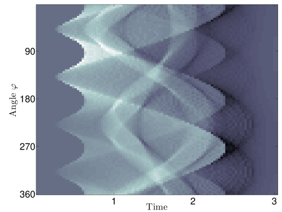
(b) Simulated pressure data.

Figure 4.1: Measurement setup and simulated data. Acoustic pressure is represented by the density in the gray scale.

4.3 Solution of the linearized inverse problem

We solve the forward problem and added random noise as described in the previous subsection. Since we use only boundary sources of illumination in our simulation this corresponds to calculating the simulated forward data

$$v\coloneqq\mathbf{W}_{\Lambda,T}\circ\mathbf{H}_{f,0}(\mu_{a},\mu_{s})+\mathrm{noise}\,.$$

In our simulations the parameters $\mu_{a}$ and $\mu_{s}$ are constant on the boundary. The linearization point $(\mu_{a}^{\star},\mu_{s}^{\star})$ is chosen spatially constant and equal to the respective parameter on the boundary. This represents a situation where the parameters of the tissue on the boundary are known but internal variations in absorption and/or scattering are of interest. The solution at the linearization point is denoted by $v^{\star}\coloneqq\mathbf{W}_{\Lambda,T}\circ\mathbf{H}_{f,0}(\mu_{a}^{\star},\mu_{s}^{\star})$. In our numerical simulations we do not attempt to reconstruct $\mu_{s}$. We linearize around the value at the boundary and fix that value for all our calculations. Reconstruction of $\mu_{s}$ is more difficult because $\mu_{s}$ influences the heating in a more indirect way. Preliminary numerical attempts indicate that different step sizes in the direction of $\mu_{a}$ and $\mu_{s}$ have to be used but reconstruction of also $\mu_{s}$ is a subject of further studies.

As in Subsection 3.3 we write $\mathbf{D}(h_{a})=(\mathbf{H}_{f,0})^{\prime}(\mu_{a}^{\star},\mu_{s}^{\star})(h_{a},0)$ for the Gâtaux derivative of $\mathbf{H}_{f,0}$ at position $(\mu_{a}^{\star},\mu_{s}^{\star})$ in direction $(h_{a},0)$; see Proposition 2.3. We refer to $\mathbf{D}$ as the linearized heating operator. The solution of the linearized inverse problem then consists in finding $h_{a}$ in the set of admissible directions, such that the residuum functional of the linearized problem is minimized,

$$\mathrm{Res}(h_{a})=\|v-v^{\star}-(\mathbf{W}_{\Lambda,T}\circ\mathbf{D})(h_{a})\|^{2}_{2}\rightarrow\min\,.$$ (4.3)

Using the minimizer of the linearized residuum we define the approximate linearized solution as $\mu_{a}=\mu_{a}^{\star}+h_{a}$.

For solving (4.3) we use the Landweber iteration

$$h^{n+1}_{a}=h_{a}^{n}+\lambda\,\mathbf{D}^{\ast}\circ\mathbf{W}_{\Lambda,T}^{\ast}\left(v-v^{\star}-(\mathbf{W}_{\Lambda,T}\circ\mathbf{D})(h_{a}^{n})\right)\quad\text{ for }n\in\mathbb{N}\,,$$ (4.4)

with starting value $h_{a}^{0}=0$, where $\lambda$ is the step size. Note that we do not reconstruct the heating as intermediate step but immediately reconstruct the parameters of interest. Such a single stage approach has advantages especially in the case of multiple measurements with partial data; a more thorough discussion can be found in [42] for example. The heating operator is discretized with the same finite element technique as the forward-problem (see Proposition 2.3) and the adjoint is calculated after discretization as an adjoint matrix. To solve the adjoint wave propagation problem we discretize formula (2.12).

Our stability analysis shows that $\mathbf{W}_{\Lambda,T}\circ\mathbf{D}$ is Fredholm operator (see Theorem 3.8) and, in particular, that $\mathbf{W}_{\Lambda,T}\circ\mathbf{D}$ has closed range. Therefore, for any $v\in L^{2}(\Lambda\times(0,T))$, the Landweber iteration converges to the minimizer of (4.3) with a linear rate of convergence, provided that the step size satisfies $\lambda<2/\|\mathbf{W}_{\Lambda,T}\circ\mathbf{D}\|_{2}^{2}$. In the numerical simulations we used about $50$ iterations after which we already obtained quite accurate results. The convergence speed can further be accelerated by using iterations such as the CG algorithm. See [43] for a comparison and analysis of various iterative methods for the wave inversion process. Theorem 3.8 further implies that the minimizer of (4.3) is unique and satisfies the two-sided stability estimates if (3.17) is satisfied. Evaluated at the linearization point $\mu^{\star}$ inequality (3.17) reads $2\pi\,\|\mu_{a}^{\star}\|_{\infty}\,e^{\|\mu_{s}^{\star}\ell_{+}\|_{\infty}}\,\operatorname{diam}(\Omega)\,\|\Phi^{\star}\|_{\infty}<\min_{x\in\Omega}\left\{\int_{\mathbb{S}^{1}}\Phi^{\star}(x,\theta)\mathrm{d}\theta\right\}$. Assuming, as is reasonable for collinear illumination, that $\Phi^{\star}$ takes its maximum at the boundary we find $2\pi\,\operatorname{diam}(\Omega)\,\|\Phi^{\star}\|_{\infty}=I_{0}N_{\theta}2\sqrt{2}$. Here we have taken $f$ as in (4.2) which satisfies $\|f\|_{\infty}=I_{0}N_{\theta}/(2\pi)$. Geometric considerations show that maximum of $\ell_{+}$ is taken at the center where it takes the value $4\operatorname{arsinh}(1)/\pi$. So, for constant $\mu_{s}^{\star}$ and $N_{\theta}=64$, the above inequality simplifies to

$$\|\mu_{a}^{\star}\|_{\infty}\cdot 3^{\mu_{s}^{\star}}\lesssim\frac{1}{181\,I_{0}}\min_{x\in\Omega}\left\{\int_{\mathbb{S}^{1}}\Phi^{\star}(x,\theta)\mathrm{d}\theta\right\}\,.$$ (4.5)

Condition (4.5) requires quite small values for absorption and scattering at the linearization point and future work will be done to weaken this condition.

4.4 Numerical results

The domain $\Omega=[-1,1]^{2}$ is discretized by a mesh of triangular elements of 6400 degrees of freedom and we divide the angular domain into $N_{\theta}=64$ sub-intervals of equal length. The anisotropy factor is taken as $g=0.8$ throughout all the experiments.

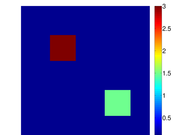
(a) Phantom $\mu_{a}$

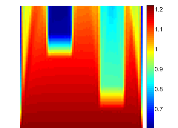
(b) Illumination

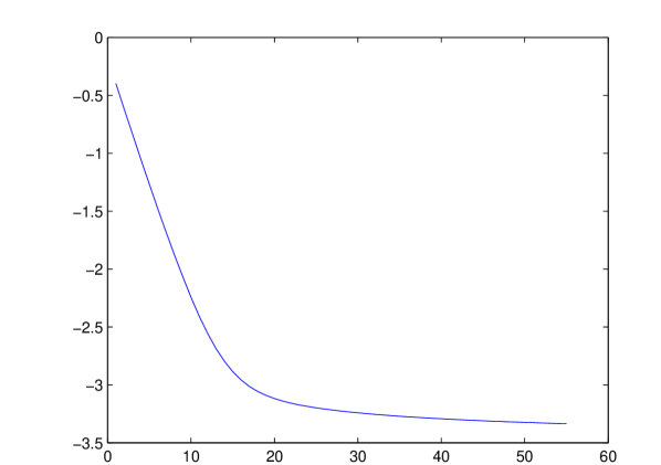
(c) Residual.

(d) Full data

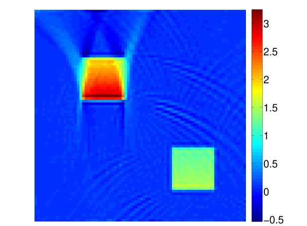
(e) Half data.

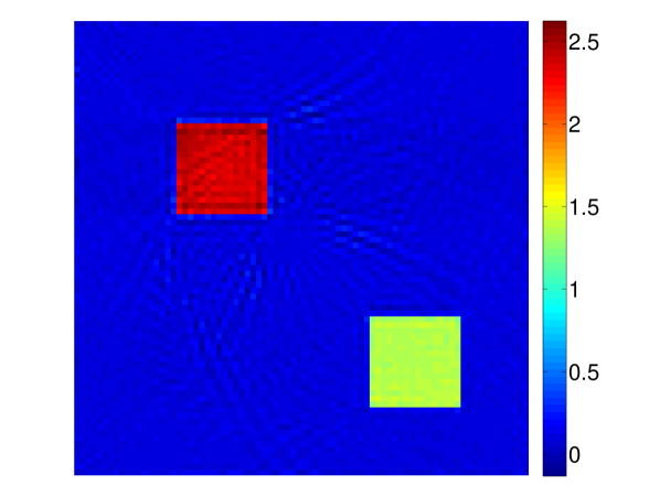
(f) 4 $\times$ half data.

Figure 4.2: Simulation results for low scattering. The scattering coefficient $\mu_{s}=0.1$ is taken constant; the absorption coefficient is shown in 2(a), and the linearization point is given by $\mu_{a}^{\star}=\mu_{s}^{\star}=0.1$.

Small scattering and good contrast in absorbtion

We first consider a rather small and constant scattering $\mu_{s}=0.1$ and good contrast in the absorption, where $\mu_{a}$ was chosen $0.1$ for the background and $1.5$ respectively $3$ in the small boxes in the interior. Observe that this corresponds to low scattering regime, as can be seen by the very well defined shadows behind the obstacles shown in Figure 4.2. The Landweber iteration (4.4) has been applied with the linearization point is $\mu_{a}^{\star}=0.1$ and $\mu_{s}^{\star}=0.1$. The reconstruction for single illumination where pressure measurements are made on the whole circle $\partial B_{1.5}(0)$ surrounding the obstacle is shown in Figure 2(d). All the singularities in $\mu_{a}$ are well resolved. Convergence of the Landweber iteration is fast but we can not expect the residuum functional (4.3) to go to zero as the data may be outside the range of the linearized forward operator. The reconstruction is qualitatively and quantitatively in good accordance with the phantom. Figure 2(e) shows the result for partial acoustic measurements, where the acoustic measurements are made on a semi-circle on the same side as the illumination. Finally, Figure 2(f) uses four consecutive illuminations with partial data (again on a semi-circle on the same side as the illumination). This has been implemented by turning the obstacle (or the measurement apparatus) by $\pi/2$ between consecutive illuminations. One notices that for a single illumination the phantom is still quite well resolved, but the typical partial data artifacts can be observed. These artifacts disappear when incomplete data from multiple measurements are collected in such a way that the union of the observation sets form the whole circle. Due to the illumination from four sides the reconstruction is even much better than in the case of one measurement with full data.

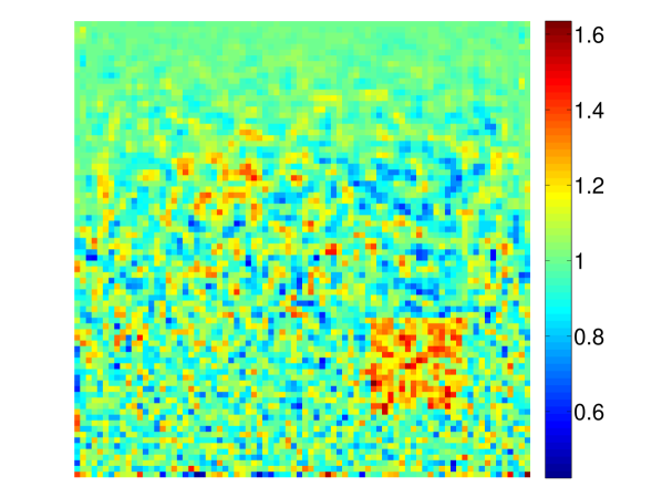
(a) Full data

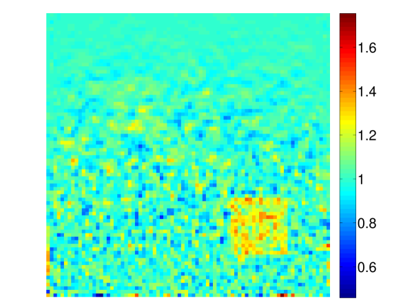
(b) Half data

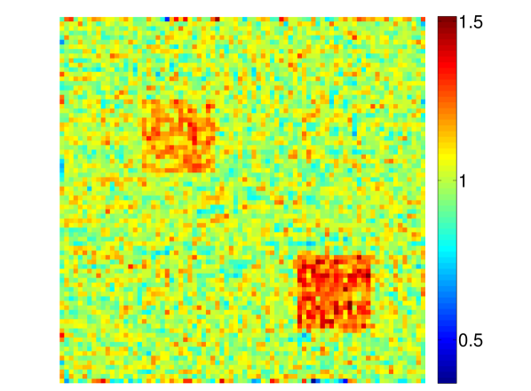
(c) 4 $\times$ half data

Figure 4.3: Reconstruction of low contrast phantom from data with large noise. The actual and linearized scattering parameters have been taken constant and equal to $\mu_{s}=\mu_{s}^{\star}=0.1$.

Low contrast phantom and large noise

For the experiment presented next we decrease the contrast in $\mu_{a}$. To demonstrate the stability of our reconstruction approach we also increase the noise. The scattering parameter $\mu_{s}=0.1$, constant throughout the domain, and the absorption coefficient $\mu_{a}$ is chosen to take the value 1 in the background, and $1.1$ respectively $1.2$ in the obstacles. The noise has a standard deviation of $5\%$. The reconstruction results are shown in Figure 4.3. One notices that the upper left square of very low contrast is only barely visible in the full data situation and probably not recognizable if the phantom is unknown. As expected multiple measurements from different directions increase the signal to noise ratio even if only incomplete data is acquired.

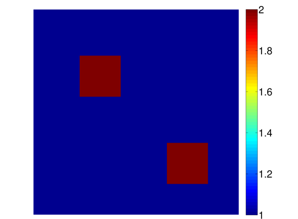
(a) Phantom

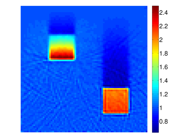
(b) Full data

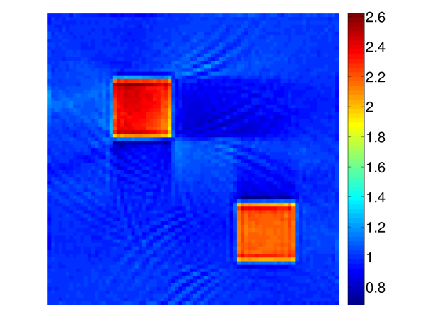
(c) 4 $\times$ half data

Figure 4.4: Reconstruction for increased scattering.The actual absorption and scattering coefficients are shown in the first to pictures and the linearization points have been taken as $\mu_{a}^{\star}=1$ and $\mu_{s}^{\star}=1$.

Increased scattering

In our final experiment we investigate the effect of large scattering. We use the value $1$ for $\mu_{s}$ in the background, and the values $1$ and $8$ in the upper left and lower right obstacle, respectively. The absorption $\mu_{a}$ is chosen equal to $1$ in the background and $2$ in the obstacles. To show the consequences of a wrong guess for the linearization point in $\mu_{s}$ we choose the linearization point to be $\mu_{a}^{\star}=1$ and $\mu_{s}^{\star}=1$. In particular, the actual and linearized scattering coefficients take different valued in the upper left box. The noise standard deviation is taken as $0.5\%$.

Reconstruction results are shown in Figure 4.4. It can be seen that also for larger scattering the edges of the squares are well resolved and the quantitative agreement of the reconstruction is still quite good. If the scattering rate in the interior is larger and thus the linearization point is chosen wrong then the algorithm has a tendency to overestimate the absorption. This is due to the fact that a larger scattering rate also leads to larger absorption by lowering the mean free path and thus potentially increasing the length that light has to travel to pass a high scattering area. Note also that in the vicinity of high scattering areas the intensity increases because light is scattered out of that area with larger probability than in the other direction. Thus the absorption in areas close to high scattering areas is underestimated and the absorption inside is overestimated. This phenomenon can be seen quite well in the upper left rectangle in Figure 4.4.

5 Conclusion and outlook

In this paper we have studied the linearized inverse problem of qPAT using single as well a multiple illumination. We employed the RTE as accurate model for light propagation in the framework of the single stage approach introduced in [42]. We have shown that the linearized heating operator $\mathbf{D}$ is an elliptic pseudodifferential operator of order zero provided that the background fluence is non-vanishing (see Theorems 3.3 and 3.8). This in particular implies the stability of the generalized (Moore-Penrose) inverse of $\mathbf{D}$. Further, we were able to show injectivity and two-sided stability estimates for the linearized inverse problem using single as well a multiple illuminations. These results are presented in Theorems 3.5 and 3.6 for non-vanishing scattering, in Theorem 3.8) for vanishing scattering, and in Theorem  3.9 for multiple illuminations. In the case of non-vanishing scattering our condition guaranteeing injectivity requires quite small values of scattering and absorption at the linearization point. Relaxing such assumptions is an interesting line of future research. Another important aspect is the extension of our stability estimates to the fully non-linear case. Finally, investigating single state qPAT with multiple illuminations for moving object (see [20] for qualitative PAT with moving object) is also a challenging topic.

For numerical computations, the linearization simplifies matters considerable because all the matrices for the solution of the RTE have to be constructed only once. Detailed numerical simulations have been performed to demonstrate the feasibility of solving the linearized problem. From the presented numerical results we conclude that solving the linearized inverse problem gives useful quantitative reconstructions even if no attempt to reconstruct the scattering coefficient has been made. Recovering the absorption and the scattering coefficient simultaneously seems difficult because the scattering leads to a lower order contribution to the data, as can also be seen from the theoretical considerations in Section 3. Nonetheless suitable regularization and preconditioning can lead to reasonable reconstruction results. Such investigations will also be subject of further work.

Appendix A Inversion of the wave equation

Recall the operator $\mathbf{W}_{\Lambda,T}$ is defined by $\mathbf{W}_{\Lambda,T}h=p|_{\Lambda\times(0,T)}$, where $p$ is the solution of(2.9) with initial data $h$ supported inside $\Omega$ and $\Lambda\subseteq\partial D$ is a subset of the closed surface enclosing $\Omega$. Lemma 2.4 states that $\mathbf{W}_{\Lambda,T}\colon L^{2}_{\Omega}(\mathbb{R}^{d})\to L^{2}\left(\Lambda\times(0,T)\right)$ is linear and bounded. The inversion of $\mathbf{W}_{\partial D,T}$ is well studied and several efficient inversion algorithm are available. Such algorithms include explicit inversion formulas [34, 35, 58, 41, 44, 66, 68, 82], series solution [1, 40, 59, 84], time reversal methods [18, 47, 35, 75], and iterative approaches based on the adjoint [5, 15, 43, 48, 71]. For the limited data case, most of the reconstruction methods are of iterative nature (see, e.g., [5, 15, 43, 48, 71]). In this appendix, we describe some theoretical results on the inversion of $\mathbf{W}_{\Lambda,T}$ that are relevant for our purpose.

Lemma A.1 (Uniqueness of reconstruction).

The data $\mathbf{W}_{\Lambda,T}(h)$ uniquely determines $h$ on $\Omega_{\Lambda,T}\coloneqq\bigl{\{}x\in\Omega\mid\operatorname{dist}(x,\Lambda)\leq T\bigr{\}}$.

Proof.

See [35, 75]. ∎

Proposition A.1 in particular implies that $\mathbf{W}_{\Lambda,\Omega}$ is injective from $L^{2}(\Omega)$ to $L^{2}(\Lambda\times(0,T))$ if $\Omega_{\Lambda,T}=\Omega$. This holds, for example, when $T\geq\max_{x\in\Omega}\operatorname{dist}(x,\Lambda)$. However, even if the inverse operator $\mathbf{W}^{-1}$ exists, its computation may be a severely ill-posed problem. Stability of the reconstruction can be obtained if additionally the following visibility condition is satisfied.

Condition A.2 (Visibility condition).

For each $x\in\Omega$ a line passing through $x$ intersects $\Lambda$ at a point of distance less than $T$ from $x$.

Under the visibility condition the following stability result holds.

Lemma A.3 (Stability of inversion).

If the visibility condition A.2 holds, then $\mathbf{W}^{-1}_{\Lambda,T}\colon L^{2}(\Lambda\times(0,T))\to L^{2}(\Omega)$ is bounded.

Proof.

See [75]. ∎

Proposition A.3 in particular implies that under the visibility condition, the inverse operator $\mathbf{W}^{-1}_{\Lambda,T}$ is Lipschitz continuous. On the other hand, if the visibility condition does not hold, then $\mathbf{W}^{-1}_{\Lambda,T}$ is not even conditionally Hölder continuous (see [67]).

Although it is not clear how to directly evaluate $\mathbf{W}_{\Lambda,T}^{-1}$ for partial data, microlocal inversion of $\mathbf{W}_{\Lambda,T}$ is quite straight forward. That is, one can recover the visible singularities of $h$ from $\mathbf{W}_{\Lambda,T}(h)$ by a direct method. To this end, let $\chi_{\Lambda,T}\in C^{\infty}(\partial D\times[0,\infty))$ be a nonnegative function with $\mbox{supp}(\chi_{\Lambda,T})=\Lambda\times[0,T]$. Then, one can decompose

$$\chi_{\Lambda,T}\mathbf{W}_{\Lambda,T}h=\mathbf{W}^{(+)}h+\mathbf{W}^{(-)}h\,,$$

where $\mathbf{W}^{(+)},\mathbf{W}^{(-)}\colon C^{\infty}(\Omega)\to C^{\infty}(\Lambda\times(0,T))$ are Fourier integral operators of order zero. Each of them describes how the singularities of $h$ induce singularities of $\mathbf{W}_{\Lambda,T}h$. Each singularity $(x,\xi)\in\mathrm{WF}(h)$ breaks into two equal parts traveling on opposite rays $\ell_{\pm}(x,\xi)\coloneqq\{x\pm r\xi\mid r>0\}$. Those singularities hit the observation surface $\partial D$ at location $y_{\pm}(x,\xi)$ and time $t_{\pm}(x,\xi)=\left|x-y_{\pm}(x,\xi)\right|$. Their projection on the cotangent bundle of $\partial D\times(0,\infty)$ at $(y_{\pm}(x,\xi),t_{\pm}(x,\xi))$ are the induced singularities of $\chi_{\Lambda,T}\mathbf{W}_{\Lambda,T}h$ if $\chi_{\Lambda,T}(y_{+}(x,\xi),t_{+}(x,\xi))>0$ or $\chi_{\Lambda,T}(y_{-}(x,\xi),t_{-}(x,\xi))>0$. In that case, $(x,\xi)$ is called a visible singularity of $h$. Any visible singularity can be reconstructed by time-reversal, described as follows. For given data $g\colon\partial D\times(0,T)\to\mathbb{R}$, consider the time-reversed problem

$$\left\{\begin{aligned} \partial_{t}^{2}q(x,t)-\Delta q(x,t)&=0\,,&&\text{ for }\left(x,t\right)\in D\times\left(0,T\right)\\ q\left(x,T\right)=\partial_{t}q\left(x,T\right)&=0\,,&&\text{ for }x\in D\\ q\left(x,t\right)&=g(x,t)\,,&&\text{ for }(x,t)\in\partial D\times(0,T)\,.\end{aligned}\right.$$ (A.1)

We define the time reversal operator $\mathbf{A}$ by $\mathbf{A}(g)\coloneqq q(\,\cdot\,,0)$.

Lemma A.4 (Recovery of singularities).

$\mathbf{A}\chi_{\Lambda,T}\mathbf{W}_{\Lambda,T}$ is a pseudo-differential operator of order zero, whose principal symbol is $\tfrac{1}{2}\sum_{\sigma=\pm}\chi_{\Lambda,T}(y_{\sigma}(x,\xi),t_{\sigma}(x,\xi))$.

Proof.

See [75]. ∎

Let $(x,\xi)$ be a visible singularity of $h$. Since $\mathbf{A}\chi_{\Lambda,T}\mathbf{W}_{\Lambda,T}$ is positive at $(x,\xi)$, $(x,\xi)$ is also a singularity of $\mathbf{A}\chi_{\Lambda,T}\mathbf{W}_{\Lambda,T}(h)$. That is, all the visible singularities are reconstructed by the time-reversal method. We, finally, note that the multiplication with a smooth function $\chi_{\Lambda,T}$ is essential, since otherwise the time-reversal procedure introduces artifacts, see [37, 67].

References

- [1] M. Agranovsky and P. Kuchment, Uniqueness of reconstruction and an inversion procedure for thermoacoustic and photoacoustic tomography with variable sound speed, Inverse Probl., 23 (2007), pp. 2089–2102.
- [2] M. Agranovsky, P. Kuchment, and L. Kunyansky, On reconstruction formulas and algorithms for the thermoacoustic tomography, in Photoacoustic imaging and spectroscopy, L. V. Wang, ed., CRC Press, 2009, ch. 8, pp. 89–101.
- [3] H. Ammari, E. Bossy, V. Jugnon, and H. Kang, Reconstruction of the optical absorption coefficient of a small absorber from the absorbed energy density, SIAM J. Appl. Math., 71 (2011), pp. 676–693.
- [4] S. R. Arridge, Optical tomography in medical imaging, Inverse Probl., 15 (1999), pp. R41–R93.
- [5] S. R. Arridge, M. M. Betcke, B. T. Cox, F. Lucka, and B. E. Treeby, On the adjoint operator in photoacoustic tomography, Inverse Probl., 32 (2016), p. 115012 (19pp).
- [6] S. R. Arridge and J. C. Schotland, Optical tomography: forward and inverse problems, Inverse Probl., 25 (2009), p. 123010.
- [7] G. Bal, C. Guo, and F. Monard, Linearized internal functionals for anisotropic conductivities, arXiv preprint arXiv:1302.3354, (2013).
- [8] G. Bal, A. Jollivet, and V. Jugnon, Inverse transport theory of photoacoustics, Inverse Probl., 26 (2010), p. 025011.
- [9] G. Bal and A. Moradifam, Photo-acoustic tomography in a rotating measurement setting, Inverse Probl., 32 (2016), p. 105012.
- [10] G. Bal and S. Moskow, Local inversions in ultrasound-modulated optical tomography, Inverse Problems, 30 (2014), p. 025005.
- [11] G. Bal and K. Ren, Multi-source quantitative photoacoustic tomography in a diffusive regime, Inverse Probl., 27 (2011), pp. 075003, 20.
- [12] G. Bal, K. Ren, G. Uhlmann, and T. Zhou, Quantitative thermo-acoustics and related problems, Inverse Probl., 27 (2011), p. 055007.
- [13] G. Bal and T. Zhou, Hybrid inverse problems for a system of maxwell’s equations, Inverse Probl., 30 (2014), p. 055013.
- [14] P. Beard, Biomedical photoacoustic imaging, Interface focus, 1 (2011), pp. 602–631.
- [15] Z. Belhachmi, T. Glatz, and O. Scherzer, A direct method for photoacoustic tomography with inhomogeneous sound speed, Inverse Probl., 32 (2016), p. 045005.
- [16] M. Bergounioux, X. Bonnefond, T. Haberkorn, and Y. Privat, An optimal control problem in photoacoustic tomography, Math. Mod. Meth. Appl. S., 24 (2014), pp. 2525–2548.
- [17] P. Burgholzer, J. Bauer-Marschallinger, H. Grün, M. Haltmeier, and G. Paltauf, Temporal back-projection algorithms for photoacoustic tomography with integrating line detectors, Inverse Probl., 23 (2007), pp. S65–S80.
- [18] P. Burgholzer, G. J. Matt, M. Haltmeier, and G. Paltauf, Exact and approximate imaging methods for photoacoustic tomography using an arbitrary detection surface, Phys. Rev. E, 75 (2007), p. 046706.
- [19] J. Chen and Y. Yang, Quantitative photo-acoustic tomography with partial data, Inverse Probl., 28 (2012), p. 115014.
- [20] J. Chung and L. Nguyen, Motion Estimation and Correction in Photoacoustic Tomographic Reconstruction, ArXiv e-prints, (2016), https://arxiv.org/abs/1609.08529.
- [21] B. T. Cox, S. A. Arridge, and P. C. Beard, Gradient-based quantitative photoacoustic image reconstruction for molecular imaging, Proc. SPIE, 6437 (2007), p. 64371T.
- [22] B. T. Cox, S. R. Arridge, P. Köstli, and P. C. Beard, Two-dimensional quantitative photoacoustic image reconstruction of absorption distributions in scattering media by use of a simple iterative method, Appl. Opt., 45 (2006), pp. 1866–1875.
- [23] B. T. Cox, J. G. Laufer, S. R. Arridge, and P. C. Beard, Quantitative spectroscopic photoacoustic imaging: a review, J. Biomed. Opt., 17 (2012), p. 0612021.
- [24] R. Dautray and J. Lions, Mathematical analysis and numerical methods for science and technology. Vol. 6, Springer-Verlag, Berlin, 1993.
- [25] A. De Cezaro and T. F. De Cezaro, Regularization approaches for quantitative photoacoustic tomography using the radiative transfer equation, J. Math. Anal. Appl., 429 (2015), pp. 415–438.
- [26] R. DeVore and G. Petrova, The averaging lemma, J. Amer. Math. Soc., 14 (2001), pp. 279–296.
- [27] T. Ding, K. Ren, and S. Vallélian, A one-step reconstruction algorithm for quantitative photoacoustic imaging, Inverse Probl., 31 (2015), p. 095005.
- [28] O. Dorn, A transport-backtransport method for optical tomography, Inverse Probl., 14 (1998), p. 1107.
- [29] H. Egger and M. Schlottbom, Stationary radiative transfer with vanishing absorption, Math. Mod. Meth. Appl. S., 24 (2014), pp. 973–990.
- [30] H. Egger and M. Schlottbom, Numerical methods for parameter identification in stationary radiative transfer, Comput. Optim. Appl., 62 (2015), pp. 67–83.
- [31] S. Ermilov, R. Su, A. Conjusteau, F. Anis, V. Nadvoretskiy, M. Anastasio, and A. Oraevsky, Three-dimensional optoacoustic and laser-induced ultrasound tomography system for preclinical research in mice design and phantom validation, Ultrasonic imaging, 38 (2016), pp. 77–95.
- [32] L. C. Evans, Partial Differential Equations, vol. 19 of Graduate Studies in Mathematics, Amer. Math. Soc., Providence, RI, 1998.
- [33] F. Filbir, S. Kunis, and R. Seyfried, Effective discretization of direct reconstruction schemes for photoacoustic imaging in spherical geometries, SIAM J. Numer. Anal., 52 (2014), pp. 2722–2742.
- [34] D. Finch, M. Haltmeier, and Rakesh, Inversion of spherical means and the wave equation in even dimensions, SIAM J. Appl. Math., 68 (2007), pp. 392–412.
- [35] D. Finch, S. K. Patch, and Rakesh, Determining a function from its mean values over a family of spheres, SIAM J. Math. Anal., 35 (2004), pp. 1213–1240.
- [36] D. Finch and Rakesh, The spherical mean value operator with centers on a sphere, Inverse Probl., 23 (2007), pp. 37–49.
- [37] J. Frikel and E. T. Quinto, Artifacts in incomplete data tomography with applications to photoacoustic tomography and sonar, SIAM J. Appl. Math., 75 (2015), pp. 703–725.
- [38] H. Gao, J. Feng, and L. Song, Limited-view multi-source quantitative photoacoustic tomography, Inverse Probl., 31 (2015), p. 065004.
- [39] F. Golse, P. Lions, B. Perthame, and R. Sentis, Regularity of the moments of the solution of a transport equation, J. Func. Anal., 76 (1988), pp. 110–125.
- [40] M. Haltmeier, Frequency domain reconstruction for photo- and thermoacoustic tomography with line detectors, Math. Models Methods Appl. Sci., 19 (2009), pp. 283–306.
- [41] M. Haltmeier, Universal inversion formulas for recovering a function from spherical means, SIAM J. Math. Anal., 46 (2014), pp. 214–232.
- [42] M. Haltmeier, L. Neumann, and S. Rabanser, Single-stage reconstruction algorithm for quantitative photoacoustic tomography, Inverse Probl., 31 (2015), p. 065005.
- [43] M. Haltmeier and L. V. Nguyen, Iterative methods for photoacoustic tomography with variable sound speed. arXiv:1611.07563, 2016.
- [44] M. Haltmeier and S. Pereverzyev, Jr., The universal back-projection formula for spherical means and the wave equation on certain quadric hypersurfaces, J. Math. Anal. Appl., 429 (2015), pp. 366–382.
- [45] M. Haltmeier, T. Schuster, and O. Scherzer, Filtered backprojection for thermoacoustic computed tomography in spherical geometry, Math. Method. Appl. Sci., 28 (2005), pp. 1919–1937.
- [46] L. Hörmander, Fourier integral operators. I, Acta Math., 127 (1971), pp. 79–183.
- [47] Y. Hristova, P. Kuchment, and L. Nguyen, Reconstruction and time reversal in thermoacoustic tomography in acoustically homogeneous and inhomogeneous media, Inverse Probl., 24 (2008), p. 055006 (25pp).
- [48] C. Huang, K. Wang, L. Nie, and M. A. Wang, L. V.and Anastasio, Full-wave iterative image reconstruction in photoacoustic tomography with acoustically inhomogeneous media, IEEE Trans. Med. Imag, 32 (2013), pp. 1097–1110.
- [49] F. John, Partial Differential Equations, vol. 1 of Applied Mathematical Sciences, Springer Verlag, New York, fourth ed., 1982.
- [50] G. Kanschat, Solution of radiative transfer problems with finite elements, in Numerical methods in multidimensional radiative transfer, Springer, Berlin, 2009, pp. 49–98.
- [51] R. Kowar, On time reversal in photoacoustic tomography for tissue similar to water, SIAM J. Imaging Sci., 7 (2014), pp. 509–527.
- [52] R. A. Kruger, K. K. Kopecky, A. M. Aisen, R. D. R., G. A. Kruger, and W. L. Kiser, Thermoacoustic CT with Radio waves: A medical imaging paradigm, Radiology, 200 (1999), pp. 275–278.
- [53] R. A. Kruger, P. Lui, Y. R. Fang, and R. C. Appledorn, Photoacoustic ultrasound (PAUS) – reconstruction tomography, Med. Phys., 22 (1995), pp. 1605–1609.
- [54] P. Kuchment, The Radon transform and medical imaging, vol. 85, SIAM, 2014.
- [55] P. Kuchment and L. A. Kunyansky, Mathematics of thermoacoustic and photoacoustic tomography, Eur. J. Appl. Math., 19 (2008), pp. 191–224.
- [56] P. Kuchment and D. Steinhauer, Stabilizing inverse problems by internal data, Inverse Probl., 28 (2012), p. 084007.
- [57] P. Kuchment and D. Steinhauer, Stabilizing inverse problems by internal data. ii: non-local internal data and generic linearized uniqueness, Anal. Math. Phys., 5 (2015), pp. 391–425.
- [58] L. A. Kunyansky, Explicit inversion formulae for the spherical mean Radon transform, Inverse Probl., 23 (2007), pp. 373–383.
- [59] L. A. Kunyansky, A series solution and a fast algorithm for the inversion of the spherical mean Radon transform, Inverse Probl., 23 (2007), pp. S11–S20.
- [60] Y. Lou, K. Wang, A. A. Oraevsky, and M. A. Anastasio, Impact of nonstationary optical illumination on image reconstruction in optoacoustic tomography, J. Opt. Soc. Am. A, 33 (2016), pp. 2333–2347.
- [61] A. V. Mamonov and K. Ren, Quantitative photoacoustic imaging in radiative transport regime, Comm. Math. Sci., 12 (2014), pp. 201–234.
- [62] S. McDowall, P. Stefanov, and A. Tamasan, Stability of the gauge equivalent classes in inverse stationary transport, Inverse Probl., 26 (2010), p. 025006.
- [63] M. Mokthar-Kharroubi, Mathematical topics in neutron transport theory, World Scientific, 1997.
- [64] C. Montalto and P. Stefanov, Stability of coupled-physics inverse problems with one internal measurement, Inverse Probl., 29 (2013), p. 125004.
- [65] W. Naetar and O. Scherzer, Quantitative photoacoustic tomography with piecewise constant material parameters, SIAM J. Imaging Sci., 7 (2014), pp. 1755–1774.
- [66] F. Natterer, Photo-acoustic inversion in convex domains, Inverse Probl. Imaging, 6 (2012), pp. 315–320.
- [67] L. Nguyen, On singularities and instability of reconstruction in thermoacoustic tomography, Tomography and inverse transport theory, Contemp. Math., 559 (2011), pp. 163–170.
- [68] L. V. Nguyen, A family of inversion formulas for thermoacoustic tomography, Inverse Probl. Imaging, 3 (2009), pp. 649–675.
- [69] L. V. Nguyen and L. A. Kunyansky, A dissipative time reversal technique for photoacoustic tomography in a cavity, SIAM J. Imaging Sci., 9 (2016), pp. 748–769.
- [70] K. Ren, H. Gao, and H. Zhao, A hybrid reconstruction method for quantitative PAT, SIAM J. Imaging Sci., 6 (2013), pp. 32–55.
- [71] A. Rosenthal, V. Ntziachristos, and D. Razansky, Acoustic inversion in optoacoustic tomography: A review, Curr. Med. Imaging Rev., 9 (2013), pp. 318–336.
- [72] A. Rosenthal, D. Razansky, and V. Ntziachristos, Fast semi-analytical model-based acoustic inversion for quantitative optoacoustic tomography, IEEE Trans. Med. Imag., 29 (2010), pp. 1275–1285.
- [73] T. Saratoon, T. Tarvainen, B. T. Cox, and S. R. Arridge, A gradient-based method for quantitative photoacoustic tomography using the radiative transfer equation, Inverse Probl., 29 (2013), p. 075006.
- [74] P. Stefanov and G. Uhlmann, Optical tomography in two dimensions, Meth. Appl. Anal., 10 (2003), pp. 001–010.
- [75] P. Stefanov and G. Uhlmann, Thermoacoustic tomography with variable sound speed, Inverse Probl., 25 (2009), pp. 075011, 16.
- [76] T. Tarvainen, B. T. Cox, J. P. Kaipio, and S. A. Arridge, Reconstructing absorption and scattering distributions in quantitative photoacoustic tomography, Inverse Probl., 28 (2012), p. 084009.
- [77] M. E. Taylor, Pseudodifferential operators, volume 34 of princeton mathematical series, 1981.
- [78] F. Trèves, Introduction to pseudodifferential and Fourier integral operators Volume 1: pseudodifferential operators, vol. 1, Springer Science & Business Media, 1980.
- [79] K. Wang and M. Anastasio, Photoacoustic and thermoacoustic tomography: Image formation principles, in Handbook of Mathematical Methods in Imaging, Springer, 2011, ch. 18, pp. 781–815.
- [80] L. V. Wang, Multiscale photoacoustic microscopy and computed tomography, Nat. Photonics, 3 (2009), pp. 503–509.
- [81] T. Widlak and O. Scherzer, Stability in the linearized problem of quantitative elastography, Inverse Probl., 31 (2015), p. 035005.
- [82] M. Xu and L. V. Wang, Universal back-projection algorithm for photoacoustic computed tomography, Phys. Rev. E, 71 (2005), p. 016706.
- [83] M. Xu and L. V. Wang, Photoacoustic imaging in biomedicine, Rev. Sci. Instrum., 77 (2006), p. 041101.
- [84] Y. Xu, M. Xu, and L. V. Wang, Exact frequency-domain reconstruction for thermoacoustic tomography–II: Cylindrical geometry, IEEE Trans. Med. Imag., 21 (2002), pp. 829–833.
- [85] L. Yao, Y. Sun, and J. Huabei, Transport-based quantitative photoacoustic tomography: simulations and experiments, Phys. Med. Biol., 55 (2010), pp. 1917–1934.
- [86] Z. Yuan and H. Jiang, A calibration-free, one-step method for quantitative photoacoustic tomography, Med. Phys., 39 (2012), pp. 6895–6899.