A new class of robust two-sample Wald-type tests

Abhik Ghosh1βˆ—, Nirian Martin2, Ayanendranath Basu1 and Leandro Pardo2
1 Indian Statistical Institute, Kolkata, India
2 Complutense University, Madrid, Spain
βˆ—Corresponding author; Email: abhianik@gmail.com
Abstract

Parametric hypothesis testing associated with two independent samples arises frequently in several applications in biology, medical sciences, epidemiology, reliability and many more. In this paper, we propose robust Wald-type tests for testing such two sample problems using the minimum density power divergence estimators of the underlying parameters. In particular, we consider the simple two-sample hypothesis concerning the full parametric homogeneity of the samples as well as the general two-sample (composite) hypotheses involving nuisance parameters also. The asymptotic and theoretical robustness properties of the proposed Wald-type tests have been developed for both the simple and general composite hypotheses. Some particular cases of testing against one-sided alternatives are discussed with specific attention to testing the effectiveness of a treatment in clinical trials. Performances of the proposed tests have also been illustrated numerically through appropriate real data examples.

Keywords: Robust Hypothesis Testing; Two-Sample problems; Minimum Density Power Divergence Estimator; Influence function; Clinical Trial

1 Introduction

Testing of parametric hypothesis is an important paradigm of statistical inference. In many real life applications like medical sciences, biology, epidemiology, sociology, reliability etc., we need to compare data from two independent samples through appropriate two-sample tests of hypotheses. Examples include but not limited to comparing mean of any biomarkers or success of any treatment between control and treatment groups, comparing lifetime of two populations in reliability etc.

Mathematically, let (𝒳​, ​β𝒳, ​P𝜽)𝜽∈𝚯subscript𝒳,Β subscript𝛽𝒳 subscriptπ‘ƒπœ½πœ½πš―\left(\mathcal{X}\text{, }\beta_{\mathcal{X}},\text{ }P_{\boldsymbol{{\boldsymbol{\theta}}}}\right)_{\boldsymbol{{\boldsymbol{\theta}}}\mathbf{\in}\boldsymbol{\Theta}} be the statistical space associated with the random variable X,𝑋X{,} where β𝒳subscript𝛽𝒳\beta_{\mathcal{X}} is the ΟƒπœŽ\sigma-field of Borel subsets AβŠ‚π’³π΄π’³A\subset\mathcal{X} and {P𝜽}𝜽∈𝚯subscriptsubscriptπ‘ƒπœ½πœ½πš―\left\{P_{\boldsymbol{{\boldsymbol{\theta}}}}\right\}_{\boldsymbol{{\boldsymbol{\theta}}}\in\boldsymbol{\Theta}} is a family of probability distributions defined on the measurable space (𝒳​, ​β𝒳)𝒳,Β subscript𝛽𝒳\left(\mathcal{X}\text{, }\beta_{\mathcal{X}}\right) where 𝚯𝚯\boldsymbol{\Theta} is an open subset of ℝpsuperscriptℝ𝑝\mathbb{R}^{p}, with pβ‰₯1.𝑝1p\geq 1. Probability measures P𝜽subscriptπ‘ƒπœ½P_{\boldsymbol{{\boldsymbol{\theta}}}} are assumed to be described by densities fπœ½β€‹(x)=d​P𝜽/d​μ​(x),subscriptπ‘“πœ½π‘₯𝑑subscriptπ‘ƒπœ½π‘‘πœ‡π‘₯f_{\boldsymbol{{\boldsymbol{\theta}}}}\left(x\right)=dP_{\boldsymbol{{\boldsymbol{\theta}}}}/d\mu\left(x\right), where ΞΌπœ‡\mu is a ΟƒπœŽ\sigma-finite measure on (𝒳​, ​β𝒳).𝒳,Β subscript𝛽𝒳\left(\mathcal{X}\text{, }\beta_{\mathcal{X}}\right). We shall denote by β„±={f𝜽:πœ½βˆˆπš―βŠ‚β„p}β„±conditional-setsubscriptπ‘“πœ½πœ½πš―superscriptℝ𝑝\mathcal{F}=\left\{f_{\boldsymbol{{\boldsymbol{\theta}}}}:~{}\boldsymbol{{\boldsymbol{\theta}}\in\Theta\subset}\mathbb{R}^{p}\right\} a set of parametric model densities. On the basis of two independent random samples X1,…,Xnsubscript𝑋1…subscript𝑋𝑛X_{1},...,X_{n} and Y1,….,YmY_{1},....,Y_{m} of sizes n𝑛n and mπ‘šm, respectively, from two densities f𝜽1​(x)subscript𝑓subscript𝜽1π‘₯f_{\mathbf{{\boldsymbol{\theta}}}_{1}}\left(x\right) and f𝜽2​(x)subscript𝑓subscript𝜽2π‘₯f_{\mathbf{{\boldsymbol{\theta}}}_{2}}\left(x\right) belonging to β„±β„±\mathcal{F}, we can solve the problem of complete homogeneity by testing

H0:𝜽1=𝜽2​ versus ​H1:𝜽1β‰ πœ½2.:subscript𝐻0subscript𝜽1subscript𝜽2Β versusΒ subscript𝐻1:subscript𝜽1subscript𝜽2H_{0}:\boldsymbol{{\boldsymbol{\theta}}}_{1}=\boldsymbol{{\boldsymbol{\theta}}}_{2}\text{ versus }H_{1}:\boldsymbol{{\boldsymbol{\theta}}}_{1}\neq\boldsymbol{{\boldsymbol{\theta}}}_{2}. (1)

The classical test statistics for solving the problem of testing given in (1) are the likelihood ratio test, Wald test and Rao test and the unknown parameters are estimated on the basis of the maximum likelihood estimator (MLE). Some new tests statistics have been presented in the literature based on divergence measures; see for instance Basu etΒ al. (2011) and Pardo (2006). It is well-known that the MLE is a BAN estimator, i.e., is efficient asymptotically but at the same time it has serious problems of robustness. In order to avoid that problem, it has been introduced in the statistical literature some procedures of testing based on estimators with good behavior in relation to the robustness. In Basu etΒ al. (2013) the problem considered in (1) was studied on the basis of the density power divergence. They introduced a family of test statistics based on the density power divergence between $f_{\mathbf{{\boldsymbol{\theta}}}_{1}}$ and $f_{\mathbf{{\boldsymbol{\theta}}}_{2}}$ when the parameters are estimated considering the minimum density power divergence estimator (MDPDE) of Basu etΒ al. (1998). For more details about MDPDE see Section 1.1.

After solving the problem considered in (1), we will be able to test in normal populations, i.e., $f_{\mathbf{{\boldsymbol{\theta}}}_{1}}\equiv N(\mu_{1},\sigma_{1})$ and $f_{\mathbf{{\boldsymbol{\theta}}}_{2}}\equiv N(\mu_{2},\sigma_{2}),$ the following problem of complete homogeneity

H0:(ΞΌ1,Οƒ1)=(ΞΌ2,Οƒ2)​ versus ​H1:(ΞΌ1,Οƒ1)β‰ (ΞΌ2,Οƒ2).:subscript𝐻0subscriptπœ‡1subscript𝜎1subscriptπœ‡2subscript𝜎2Β versusΒ subscript𝐻1:subscriptπœ‡1subscript𝜎1subscriptπœ‡2subscript𝜎2H_{0}:(\mu_{1},\sigma_{1})=\left(\mu_{2},\sigma_{2}\right)\text{ versus }H_{1}:(\mu_{1},\sigma_{1})\neq\left(\mu_{2},\sigma_{2}\right).

But there are other interesting problems of homogeneity, for instance, to test

H0:ΞΌ1=ΞΌ2​ versus ​H1:ΞΌ1β‰ ΞΌ2:subscript𝐻0subscriptπœ‡1subscriptπœ‡2Β versusΒ subscript𝐻1:subscriptπœ‡1subscriptπœ‡2H_{0}:\mu_{1}=\mu_{2}\text{ versus }H_{1}:\mu_{1}\neq\mu_{2}

when the variance is the same but unknown, i.e., general composite hypothesis with two samples. This problem with normal population has been considered in Basu etΒ al. (2015) on the basis of introducing a family of test statistics based on the density power divergence measure and estimating the unknown parameters using the MDPDE. The results obtained were excellent in relation to the robustness and efficiency since some tests were presented in which the lost of efficiency in relation to the size and the power was not important but the increase of robustness was very significant. One can think that the problems considered previously can be solved in that way in a very satisfactory way and from a theoretical point of view it is true but from a practical point of view sometimes it is not very easy to get the density power divergence measure between $f_{\mathbf{{\boldsymbol{\theta}}}_{1}}$ and $f_{\mathbf{{\boldsymbol{\theta}}}_{2}}.$ In this paper we are going to present a family of test statistics which are easy to calculate based on the MDPDE for any general two-sample problems with any parametric distribution. These test statistics are called Wald-type test statistics and their usefulness have been illustrated in the literature of one sample testing problems by Basu etΒ al. (2016) and Ghosh et al. (2016). In the present paper, not only we shall present the asymptotic distribution of the Wald-type test statistics for two-sample problems but also a theoretical study of the robustness properties of them along with suitable examples and numerical illustrations.

The rest of the paper is organized as follows: In Section 1.1 we present some results in relation to the MDPDE that will be necessary for the rest of the paper. Section 2 is devoted to present the family of Wald-type tests for solving the problem of complete homogeneity, i.e., the problem considered in (1). After defining the Wald-type tests based on MDPDE, we study its asymptotic distribution as well as the theoretical robustness properties with examples. In Section 3, we present a family of Wald-type tests for general composite hypotheses in two sample context. We shall derive the asymptotic distribution of the Wald-type tests introduced as well as its robustness properties. Illustrations will be provided for the special case of testing partial homogeneity in presence of nuisance parameters like, for example, testing equality of two normal means with unknown (nuisance) variances. In Section 4, we briefly describe the extensions for testing the two-sample hypotheses against one-sided alternatives for some particular cases. Section 5 will present several real life applications of our proposal with interesting data examples from applied sciences like medical, biology, reliability etc. Appropriate simulation studies with some comments on the choice of tuning parameters will be presented in Section 6. The paper ends with a short concluding remark in Section 7. For brevity in presentation, the proofs of all the results have been moved to Appendix A.

1.1 Minimum density power divergence estimator: Asymptotic properties and robustness

Given any two densities $f_{\mathbf{{\boldsymbol{\theta}}}_{1}}$ and $f_{\mathbf{{\boldsymbol{\theta}}}_{2}}$ from $\mathcal{F}$, the density power divergence with a nonnegative tuning parameter $\beta$, is defined as (Basu etΒ al., 1998)

$$d_{\beta}(f_{\mathbf{{\boldsymbol{\theta}}}_{1}},f_{\mathbf{{\boldsymbol{\theta}}}_{2}})=\left\{\begin{array}[]{ll}\int\left\{f_{\mathbf{{\boldsymbol{\theta}}}_{2}}^{1+\beta}(x)-\left(1+\frac{1}{\beta}\right)f_{\mathbf{{\boldsymbol{\theta}}}_{2}}^{\beta}(x)f_{\mathbf{{\boldsymbol{\theta}}}_{1}}(\boldsymbol{x})+\frac{1}{\beta}f_{\mathbf{{\boldsymbol{\theta}}}_{1}}^{1+\beta}(x)\right\}dx,&\text{for}\mathrm{~{}}\beta>0,\\[8.61108pt] \int f_{\mathbf{{\boldsymbol{\theta}}}_{1}}(x)\mathrm{ln}\left(\frac{f_{\mathbf{{\boldsymbol{\theta}}}_{1}}(x)}{f_{\mathbf{{\boldsymbol{\theta}}}_{2}}(x)}\right)dx,&\text{for}\mathrm{~{}}\beta=0.\end{array}\right.$$ (2)

The divergence corresponding to $\beta=0$ may be derived from the general case by taking the continuous limit as $\beta\rightarrow 0^{+}$, and the resulting $d_{0}(f_{\mathbf{{\boldsymbol{\theta}}}_{1}},f_{\mathbf{{\boldsymbol{\theta}}}_{2}})$ turns out to be the Kullback-Leibler divergence.

Let $G$ represent the distribution function corresponding to the density $g$ that generates the data. We model it by the model density $f_{\boldsymbol{\theta}}\in\mathcal{F}$ and we are interested in the estimation of $\boldsymbol{{\boldsymbol{\theta}}}$ based on an observed random sample from $g$. The corresponding minimum density power divergence functional at $G$ with tuning parameter $\beta$, denoted by $\boldsymbol{U}_{\beta}(G)$, is defined as $d_{\beta}(g,f_{\boldsymbol{U}_{\beta}(G)})=\displaystyle\min_{\boldsymbol{{\boldsymbol{{\boldsymbol{\theta}}}}}\in\Theta}d_{\beta}(g,f_{\boldsymbol{{\boldsymbol{\theta}}}})$. Therefore the MDPDE of $\boldsymbol{{\boldsymbol{\theta}}}$ with tuning parameter $\beta$ is given by $\widehat{\boldsymbol{{\boldsymbol{\theta}}}}_{\beta}=\boldsymbol{U}_{\beta}(G_{n}),$ where $G_{n}$ is the empirical distribution function associated with the observed random sample $X_{1},\ldots,X_{n}$ from the population with density $g$. As the last term of equation (2) does not depend on $\boldsymbol{{\boldsymbol{\theta}}}$, $\widehat{\boldsymbol{{\boldsymbol{\theta}}}}_{\beta}$ is given by

$\displaystyle\widehat{\boldsymbol{{\boldsymbol{\theta}}}}_{\beta}$ $\displaystyle=$ $\displaystyle\arg\min_{\boldsymbol{{\boldsymbol{\theta}}}\in\Theta}\left\{\int f_{\boldsymbol{{\boldsymbol{\theta}}}}^{1+\beta}({x})d{x}-\left(1+\frac{1}{\beta}\right)\frac{1}{n}\sum_{i=1}^{n}f_{\boldsymbol{{\boldsymbol{\theta}}}}^{\beta}(X_{i})\right\},~{}~{}~{}~{}\mbox{ if }\beta>0,$ (3)
$\displaystyle\mbox{and }~{}~{}~{}~{}~{}~{}~{}~{}~{}~{}~{}~{}~{}~{}\widehat{\boldsymbol{{\boldsymbol{\theta}}}}_{\beta}$ $\displaystyle=$ $\displaystyle\arg\min_{\boldsymbol{{\boldsymbol{\theta}}}\in\Theta}\left\{-\frac{1}{n}\sum_{i=1}^{n}\mathrm{ln}f_{\boldsymbol{{\boldsymbol{\theta}}}}(X_{i})\right\},~{}~{}~{}~{}~{}~{}~{}~{}~{}~{}~{}~{}~{}~{}~{}~{}~{}~{}~{}~{}~{}~{}~{}~{}~{}~{}~{}~{}~{}~{}~{}~{}~{}\mbox{ if }\beta=0.$ (4)

Notice that $\widehat{\boldsymbol{{\boldsymbol{\theta}}}}_{\beta}$ for $\beta=0$ coincides with the maximum likelihood estimator (MLE). Denoting

$$V_{\boldsymbol{{\boldsymbol{\theta}}}}\left(x\right)=\int f_{\boldsymbol{{\boldsymbol{\theta}}}}^{1+\beta}(\boldsymbol{x})d\boldsymbol{x-}\left(1+\frac{1}{\beta}\right)f_{\boldsymbol{{\boldsymbol{\theta}}}}^{\beta}(x),$$

expression (3) can be written as $\widehat{\boldsymbol{{\boldsymbol{\theta}}}}_{\beta}=\arg\displaystyle\min_{\boldsymbol{{\boldsymbol{\theta}}}\in\Theta}\frac{1}{n}\displaystyle\sum_{i=1}^{n}V_{\boldsymbol{{\boldsymbol{\theta}}}}(X_{i}).$ It shows that the MDPDE is an M-estimator.

The functional $\boldsymbol{T}_{\beta}(G)$ is Fisher consistent; it takes the value $\boldsymbol{{\boldsymbol{\theta}}}$0, the true value of the parameter, when the true density is a member of the model, i.e. $g=f_{\boldsymbol{{\boldsymbol{\theta}}}_{0}}$. Let us assume $g=f_{\boldsymbol{{\boldsymbol{\theta}}}_{0}}$, and define the quantities

$$\boldsymbol{J}_{\beta}\left(\boldsymbol{{\boldsymbol{\theta}}}\right)=\int\boldsymbol{u}_{\boldsymbol{{\boldsymbol{\theta}}}}(\boldsymbol{x})\boldsymbol{u}_{\boldsymbol{{\boldsymbol{\theta}}}}^{T}(\boldsymbol{x})f_{\boldsymbol{{\boldsymbol{\theta}}}}^{1+\beta}(\boldsymbol{x})d\boldsymbol{x},\text{\quad}\boldsymbol{K}_{\beta}\left(\boldsymbol{{\boldsymbol{\theta}}}\right)=\int\boldsymbol{u}_{\boldsymbol{{\boldsymbol{\theta}}}}(\boldsymbol{x})\boldsymbol{u}_{\boldsymbol{{\boldsymbol{\theta}}}}^{T}(\boldsymbol{x})f_{\boldsymbol{{\boldsymbol{\theta}}}}^{1+2\beta}(\boldsymbol{x})d\boldsymbol{x}-\boldsymbol{\xi}_{\beta}\left(\boldsymbol{{\boldsymbol{\theta}}}\right)\boldsymbol{\xi}_{\beta}^{T}\left(\boldsymbol{{\boldsymbol{\theta}}}\right),$$ (5)

where $\boldsymbol{\xi}_{\beta}\left(\boldsymbol{{\boldsymbol{\theta}}}\right)=\int\boldsymbol{u}_{\boldsymbol{{\boldsymbol{\theta}}}}(\boldsymbol{x})f_{\boldsymbol{{\boldsymbol{\theta}}}}^{1+\beta}(\boldsymbol{x})d\boldsymbol{x}$ and $\boldsymbol{u}_{\boldsymbol{{\boldsymbol{\theta}}}}(\boldsymbol{x})=\frac{\partial}{\partial\boldsymbol{{\boldsymbol{\theta}}}}\mathrm{ln}f_{\boldsymbol{{\boldsymbol{\theta}}}}(\boldsymbol{x})$. Then, following Basu etΒ al. (1998, 2011), it can be shown that, under Assumptions (D1)–(D5) of Basu etΒ al. (2011, p.Β 304) to be referred as β€œBasu et al.Β conditions” in the rest of the paper,

$$n^{1/2}({\boldsymbol{\widehat{\boldsymbol{{\boldsymbol{\theta}}}}}}_{\beta}-\boldsymbol{{\boldsymbol{\theta}}}_{0})\underset{n\rightarrow\infty}{\overset{\mathcal{L}}{\longrightarrow}}{N}(\boldsymbol{0}_{p},\boldsymbol{{\boldsymbol{\Sigma}}}_{\beta}(\boldsymbol{{\boldsymbol{\theta}}}_{0})),$$ (6)

where $\boldsymbol{{\boldsymbol{\Sigma}}}_{\beta}(\boldsymbol{{\boldsymbol{\theta}}})=\boldsymbol{J}_{\beta}^{-1}(\boldsymbol{{\boldsymbol{\theta}}})\boldsymbol{K}_{\beta}(\boldsymbol{{\boldsymbol{\theta}}})\boldsymbol{J}_{\beta}^{-1}(\boldsymbol{{\boldsymbol{\theta}}}).$ It is a simple exercise to see that for $\beta=0,$ $\boldsymbol{J}_{\beta=0}\left(\boldsymbol{{\boldsymbol{\theta}}}\right)=\boldsymbol{K}_{\beta=0}\left(\boldsymbol{{\boldsymbol{\theta}}}\right)=\boldsymbol{I}_{F}\left(\boldsymbol{{\boldsymbol{\theta}}}\right),$ being $\boldsymbol{I}_{F}\left(\boldsymbol{{\boldsymbol{\theta}}}\right)$ the Fisher information matrix associated to the model under consideration. Therefore we obtain the classical well known result,

$$n^{1/2}({\boldsymbol{\widehat{\boldsymbol{{\boldsymbol{\theta}}}}}}-\boldsymbol{{\boldsymbol{\theta}}}_{0})\underset{n\rightarrow\infty}{\overset{\mathcal{L}}{\longrightarrow}}{N}(\boldsymbol{0}_{p},\boldsymbol{I}_{F}^{-1}(\boldsymbol{{\boldsymbol{\theta}}}_{0})).$$

Next, the influence function can be used to study the robustness of the MDPDE like any other estimator or test statistic. If the influence function is bounded, the corresponding estimator or the statistic is said to have infinitesimal robustness. Therefore, the influence function particularly can be used to quantify infinitesimal robustness of an estimator or a statistic by measuring the approximate impact on an additional observation to the underlying data. More simply, the influence function $\mathcal{IF}\left(x,\boldsymbol{U}_{\beta},F_{\boldsymbol{{\boldsymbol{\theta}}}_{0}}\right)$ is the first derivative of an estimator or statistic viewed as a functional $\boldsymbol{U}_{\beta}$ and it describes the normalized influence on the estimate or statistic of an infinitesimal observation $x$. We pay special attention to the robustness of the family of Wald-type test statistics introduced in this paper. To do that it is necessary to study the robustness of the MDPDEs. In Basu etΒ al. (1998) it was established that the influence function of the minimum density power divergence functional is

$$\mathcal{IF}\left(x,\boldsymbol{U}_{\beta},F_{\boldsymbol{{\boldsymbol{\theta}}}_{0}}\right)=\lim_{\varepsilon\rightarrow 0}\frac{\boldsymbol{U}_{\beta}\left(F_{\varepsilon}\right)-\boldsymbol{U}_{\beta}\left(F_{\boldsymbol{{\boldsymbol{\theta}}}_{0}}\right)}{\varepsilon}=\boldsymbol{J}_{\beta}^{-1}(\boldsymbol{{\boldsymbol{\theta}}}_{0})\left(\boldsymbol{u}_{\boldsymbol{{\boldsymbol{\theta}}}}\left(x\right)f_{\boldsymbol{{\boldsymbol{\theta}}}_{0}}^{\beta}(x)-\boldsymbol{\xi}\left(\boldsymbol{{\boldsymbol{\theta}}}_{0}\right)\right),$$ (7)

where $F_{\varepsilon}=(1-\varepsilon)F_{\boldsymbol{{\boldsymbol{\theta}}}_{0}}+\varepsilon\wedge_{x}$ is the $\varepsilon$-contaminated distribution of $F_{\boldsymbol{{\boldsymbol{\theta}}}_{0}}$, the distribution function corresponding to $f_{\boldsymbol{\theta}}$, with respect to the point mass distribution $\wedge_{x}$ at $x$. If we assume that $\boldsymbol{J}_{\beta}($ $\boldsymbol{{\boldsymbol{\theta}}}$ ${}_{0})$ and $\boldsymbol{\xi}\left(\boldsymbol{{\boldsymbol{\theta}}}_{0}\right)$ are finite, the influence function is a bounded function of $x$ whenever $\boldsymbol{u}_{\boldsymbol{{\boldsymbol{\theta}}}}\left(x\right)f_{\boldsymbol{{\boldsymbol{\theta}}}_{0}}^{\beta}(x)$ is bounded. And this is the case for most common parametric models at $\beta>0$ implying the robustness of MDPDEs with $\beta>0$.

2 A Simple Two-Sample Problem

Let $X_{1},...,X_{n}$ and $Y_{1},...,Y_{m}$ be two samples of sizes $n$ and $m$ respectively from two populations having distribution belonging to $\mathcal{F}$ with parameters $\boldsymbol{{\boldsymbol{\theta}}}_{1}$ and $\boldsymbol{{\boldsymbol{\theta}}}_{2}$. The most common problem under this setup is to test the complete homogeneity of the two populations. But we have two different situations depending if some of the parameters are known. To clarify this point we can be interested in testing the homogeneity of two normal populations with means and variances unknown or with known variances. The problem of testing the homogeneity of two normal populations with unknown and common variance will be studied in the next Section. In general notation, we shall assume that,

$$\boldsymbol{{\boldsymbol{\theta}}}_{1}=\left(\theta_{1,1},...,\theta_{1,r},\theta_{1,r+1},...,\theta_{1,p}\right)^{T}=\left({}^{\ast}\boldsymbol{{\boldsymbol{\theta}}}_{1}^{T},^{0}\boldsymbol{{\boldsymbol{\theta}}}_{1}^{T}\right)^{T}~{}\mbox{ and }~{}\boldsymbol{{\boldsymbol{\theta}}}_{2}=\left(\theta_{21,1},...,\theta_{2,r},\theta_{2,r+1},...,\theta_{2,p}\right)^{T}=\left({}^{\ast}\boldsymbol{{\boldsymbol{\theta}}}_{2}^{T},^{0}\boldsymbol{{\boldsymbol{\theta}}}_{2}^{T}\right)^{T}~{}~{}~{}~{}~{}$$

with ${}^{0}\boldsymbol{{\boldsymbol{\theta}}}_{1}$ and ${}^{0}\boldsymbol{{\boldsymbol{\theta}}}_{2}$ known $(p-r)$-vectors. Based on $X_{1},...,X_{n}$ we can get the MLE, ${}^{\ast}\widehat{\boldsymbol{{\boldsymbol{\theta}}}}_{1},$ of ${}^{\ast}\boldsymbol{{\boldsymbol{\theta}}}_{1}$ and based on $Y_{1},...,Y_{m}$ the MLE, ${}^{\ast}\widehat{\boldsymbol{{\boldsymbol{\theta}}}}_{2},$ of ${}^{\ast}\boldsymbol{{\boldsymbol{\theta}}}_{2}$. Assuming ${}^{\ast}\boldsymbol{{\boldsymbol{\theta}}}_{1}=^{\ast}\boldsymbol{{\boldsymbol{\theta}}}_{2}$ we can obtain an estimator, ${}_{\left(o\right)}^{\ast}\widehat{\boldsymbol{{\boldsymbol{\theta}}}}_{1}$ of the common value ${}^{\ast}\boldsymbol{{\boldsymbol{\theta}}}_{1}$ by using the two random samples $X_{1},...,X_{n}$ and $Y_{1},...,Y_{m}$ together. It is well-known that, under ${}^{\ast}\boldsymbol{{\boldsymbol{\theta}}}_{1}=^{\ast}\boldsymbol{{\boldsymbol{\theta}}}_{2}$,

$$\sqrt{\frac{mn}{m+n}}\left({}^{\ast}\widehat{\boldsymbol{{\boldsymbol{\theta}}}}_{1}-^{\ast}\widehat{\boldsymbol{{\boldsymbol{\theta}}}}_{2}\right)\underset{n\rightarrow\infty}{\overset{\mathcal{L}}{\longrightarrow}}\mathcal{N}(\boldsymbol{0}_{r},\omega\boldsymbol{I}_{F}^{-1}(^{\ast}\boldsymbol{{\boldsymbol{\theta}}}_{1},^{0}\boldsymbol{{\boldsymbol{\theta}}}_{1})+\left(1-\omega\right)\boldsymbol{I}_{F}^{-1}(^{\ast}\boldsymbol{{\boldsymbol{\theta}}}_{1},^{0}\boldsymbol{{\boldsymbol{\theta}}}_{2}))$$ (8)

with

$$\omega=\lim_{m,n\rightarrow\infty}\frac{m}{m+n}.$$

Based on (8) we can consider the Wald test for testing

H0:βˆ—πœ½1=βˆ—πœ½2Β versusΒ H1:βˆ—πœ½1β‰ βˆ—πœ½2,H_{0}:^{\ast}\boldsymbol{{\boldsymbol{\theta}}}_{1}=^{\ast}\boldsymbol{{\boldsymbol{\theta}}}_{2}\text{ versus }H_{1}:^{\ast}\boldsymbol{{\boldsymbol{\theta}}}_{1}\neq^{\ast}\boldsymbol{{\boldsymbol{\theta}}}_{2},
$\displaystyle\mbox{given by }~{}~{}~{}~{}~{}~{}W_{m,n}$ $\displaystyle=$ $\displaystyle\frac{mn}{m+n}\left({}^{\ast}\widehat{\boldsymbol{{\boldsymbol{\theta}}}}_{1}-^{\ast}\widehat{\boldsymbol{{\boldsymbol{\theta}}}}_{2}\right)^{T}\left(\frac{m\boldsymbol{I}_{F}^{-1}(^{\ast}\widehat{\boldsymbol{{\boldsymbol{\theta}}}}_{1},^{0}\boldsymbol{{\boldsymbol{\theta}}}_{1})}{m+n}+\frac{n\boldsymbol{I}_{F}^{-1}(^{\ast}\widehat{\boldsymbol{{\boldsymbol{\theta}}}}_{2},^{0}\boldsymbol{{\boldsymbol{\theta}}}_{2})}{m+n}\right)^{-1}\left({}^{\ast}\widehat{\boldsymbol{{\boldsymbol{\theta}}}}_{1}-^{\ast}\widehat{\boldsymbol{{\boldsymbol{\theta}}}}_{2}\right)~{}~{}~{}~{}~{}~{}~{}~{}~{}~{}~{}~{}~{}~{}~{}~{}~{}~{}~{}~{}~{}~{}$
$\displaystyle=$ $\displaystyle mn\left({}^{\ast}\widehat{\boldsymbol{{\boldsymbol{\theta}}}}_{1}-^{\ast}\widehat{\boldsymbol{{\boldsymbol{\theta}}}}_{2}\right)^{T}\left(m\boldsymbol{I}_{F}^{-1}(^{\ast}\widehat{\boldsymbol{{\boldsymbol{\theta}}}}_{1},^{0}\boldsymbol{{\boldsymbol{\theta}}}_{1})+n\boldsymbol{I}_{F}^{-1}(^{\ast}\widehat{\boldsymbol{{\boldsymbol{\theta}}}}_{2},^{0}\boldsymbol{{\boldsymbol{\theta}}}_{2})\right)^{-1}\left({}^{\ast}\widehat{\boldsymbol{{\boldsymbol{\theta}}}}_{1}-^{\ast}\widehat{\boldsymbol{{\boldsymbol{\theta}}}}_{2}\right).$

We can observe that in the case that $r=p$ we have $\boldsymbol{I}_{F}^{-1}(^{\ast}\boldsymbol{{\boldsymbol{\theta}}}_{1},^{0}\boldsymbol{{\boldsymbol{\theta}}}_{1})=\boldsymbol{I}_{F}^{-1}(^{\ast}\boldsymbol{{\boldsymbol{\theta}}}_{1},^{0}\boldsymbol{{\boldsymbol{\theta}}}_{2})=\boldsymbol{I}_{F}^{-1}(\boldsymbol{{\boldsymbol{\theta}}}_{0}),$ with $\boldsymbol{{\boldsymbol{\theta}}}_{1}=\boldsymbol{{\boldsymbol{\theta}}}_{2}=\boldsymbol{{\boldsymbol{\theta}}}_{0}$ and the Wald test is given by

$$W_{m,n}=\frac{mn}{m+n}\left(\widehat{\boldsymbol{{\boldsymbol{\theta}}}}_{1}-\widehat{\boldsymbol{{\boldsymbol{\theta}}}}_{2}\right)^{T}\boldsymbol{I}_{F}(^{(0)}\widehat{\boldsymbol{{\boldsymbol{\theta}}}})\left(\widehat{\boldsymbol{{\boldsymbol{\theta}}}}_{1}-\widehat{\boldsymbol{{\boldsymbol{\theta}}}}_{2}\right),$$ (9)

where ${}^{(0)}\widehat{\boldsymbol{{\boldsymbol{\theta}}}}$ denotes the MLE of $\boldsymbol{{\boldsymbol{\theta}}}_{0}$ based on the pooled sample.

Based on (8) in the case of two normal populations, with known variances $\sigma_{1}^{2}$ and $\sigma_{2}^{2}$, we can test $H_{0}:\mu_{1}=\mu_{2}.$ In this case

$$W_{m,n}=mn\frac{\left(\widehat{\mu}_{1}-\widehat{\mu}_{2}\right)^{2}}{m\sigma_{1}^{2}+n\sigma_{2}^{2}}=\frac{\left(\widehat{\mu}_{1}-\widehat{\mu}_{2}\right)^{2}}{\frac{\sigma_{1}^{2}}{n}+\frac{\sigma_{2}^{2}}{m}}.$$

Although it has several nice optimum properties, it is highly non-robust in presence of outliers even in any one sample. Here, we will generalize this Wald test to make it robust by replacing the MLE by the corresponding MDPDEs.

In the following we shall present the results for $r=p$, i.e., to test for the hypothesis in (1). The case $r<p$ can be studied in a similar way.

Let us assume ${}^{(1)}\widehat{{\boldsymbol{\theta}}}_{\beta}$ and ${}^{(2)}\widehat{{\boldsymbol{\theta}}}_{\beta}$ denote the MDPDEs of ${\boldsymbol{\theta}}_{1}$ and ${\boldsymbol{\theta}}_{2}$ respectively, obtained by minimizing the DPD with tuning parameter $\beta$ for each of the two samples separately. Further, under the null hypothesis $H_{0}:{\boldsymbol{\theta}}_{1}={\boldsymbol{\theta}}_{2}={\boldsymbol{\theta}}_{0}$ in (1), we can consider the two samples pooled together as one i.i.d.Β sample of size $m+n$ from a population having density function $f_{{\boldsymbol{\theta}}_{0}}$; let ${}^{(0)}\widehat{{\boldsymbol{\theta}}}_{\beta}$ denote the corresponding MDPDE of ${\boldsymbol{\theta}}_{0}$ with tuning parameter $\beta$ based on the pooled sample. Note that, all the three estimators ${}^{(1)}\widehat{{\boldsymbol{\theta}}}_{\beta}$ , ${}^{(2)}\widehat{{\boldsymbol{\theta}}}_{\beta}$ and ${}^{(0)}\widehat{{\boldsymbol{\theta}}}_{\beta}$ should coincide with ${\boldsymbol{\theta}}_{0}$ asymptotically under $H_{0}$ with probability tending to one. Assuming identifiability of the model family, the difference between the two estimators ${}^{(1)}\widehat{{\boldsymbol{\theta}}}_{\beta}$ and ${}^{(2)}\widehat{{\boldsymbol{\theta}}}_{\beta}$ gives us an idea of the distinction between the two samples and hence indicate any departure from the null hypothesis. So, we define a generalized Wald-type test statistics by

$\displaystyle T_{m,n}^{(\beta)}=\frac{nm}{n+m}~{}\left({}^{(1)}\widehat{{\boldsymbol{\theta}}}_{\beta}-^{(2)}\widehat{{\boldsymbol{\theta}}}_{\beta}\right)^{T}{\boldsymbol{\Sigma}}_{\beta}\left({}^{(0)}\widehat{{\boldsymbol{\theta}}}_{\beta}\right)^{-1}\left({}^{(1)}\widehat{{\boldsymbol{\theta}}}_{\beta}-^{(2)}\widehat{{\boldsymbol{\theta}}}_{\beta}\right).$ (10)

Note that, at $\beta=0$, all the MDPDEs used coincide with corresponding MLEs and hence the generalized Wald-type test statistic $T_{m,n}^{(\beta)}$ coincides with the classical Wald test statistic $W_{m,n}$ in (9).

2.1 Asymptotic Properties

In order to perform any statistical test, we first need to derive the asymptotic distribution of the test statistics under $H_{0}$. Using the asymptotic properties of the MDPDEs presented in Section 1.1, we can easily obtain the asymptotic null distribution of the proposed test statistics $T_{m,n}^{(\beta)}$ which is presented in the following theorem. Throughout the rest of the paper, we will assume Conditions (A)–(D) of Lehmann (1983, p.Β 429) about the assumed model family which we will refer as β€œLehmann conditions”. Also, we consider the following assumption.

Assumption (A):

  1. 1.

    $\frac{m}{m+n}\rightarrow\omega\in(0,1)$ as $m,n\rightarrow\infty$

  2. 2.

    The asymptotic variance-covariance matrix ${\boldsymbol{\Sigma}}_{\beta}({\boldsymbol{\theta}})$ of the MDPDE with tuning parameter $\beta$ is continuous in ${\boldsymbol{\theta}}$.

Theorem 2.1

Suppose the model density satisfies the Lehmann and Basu et al.Β conditions, and Assumption (A) holds. Then the asymptotic distribution of $T_{m,n}^{(\beta)}$ under the null hypothesis in (2) is $\chi_{p}^{2}$, the chi-square distribution with $p$ degrees of freedom.

The asymptotic null distribution of the test in Basu etΒ al. (2013) is a linear combination of chi-square distribution and hence it is somewhat difficult to obtain the critical values of their test in practice. On the contrary, our proposed tests have a simple chi-square limit under the null hypothesis and hence are much easier to perform. Our proposal provides, in this sense, an advantageous procedure for testing.

However, when the null hypothesis is not correct, i.e., 𝜽1β‰ πœ½2subscript𝜽1subscript𝜽2{\boldsymbol{\theta}}_{1}\neq{\boldsymbol{\theta}}_{2}, then the pooled estimator ${}^{(0)}\widehat{{\boldsymbol{\theta}}}_{\beta}$ no longer converges to ${\boldsymbol{\theta}}_{1}$ or ${\boldsymbol{\theta}}_{2}$; rather it will then converges in probability to a new value ${\boldsymbol{\theta}}_{3}$, say, which is a function of ${\boldsymbol{\theta}}_{1}$, ${\boldsymbol{\theta}}_{2}$ and $\omega$. For example, if the estimators are additive in sample data, e.g.Β sample mean, then we will have ${\boldsymbol{\theta}}_{3}=(1-\omega){\boldsymbol{\theta}}_{1}+\omega{\boldsymbol{\theta}}_{2}$. Define $l_{{\boldsymbol{\theta}}_{3},\beta}^{\ast}({\boldsymbol{\theta}}_{1},{\boldsymbol{\theta}}_{2})=({\boldsymbol{\theta}}_{1}-{\boldsymbol{\theta}}_{2})^{T}{\boldsymbol{\Sigma}}_{\beta}({\boldsymbol{\theta}}_{3})^{-1}({\boldsymbol{\theta}}_{1}-{\boldsymbol{\theta}}_{2}).$ Then we have the following result.

Theorem 2.2

Suppose the model density satisfies the Lehmann and Basu et al.Β conditions, and Assumption (A) holds. Then, as $m,n\rightarrow\infty$, we have for any ${\boldsymbol{\theta}}_{1}\neq{\boldsymbol{\theta}}_{2}$

$\displaystyle\sqrt{\frac{mn}{m+n}}\left[l_{{}^{(0)}\widehat{{\boldsymbol{\theta}}}_{\beta},\beta}^{\ast}(^{(1)}\widehat{{\boldsymbol{\theta}}}_{\beta},^{(2)}\widehat{{\boldsymbol{\theta}}}_{\beta})-l_{{\boldsymbol{\theta}}_{3},\beta}^{\ast}({\boldsymbol{\theta}}_{1},{\boldsymbol{\theta}}_{2})\right]\underset{m,n\rightarrow\infty}{\overset{\mathcal{L}}{\longrightarrow}}N\left(0,4\sigma_{{\boldsymbol{\theta}}_{3},\beta}^{2}({\boldsymbol{\theta}}_{1},{\boldsymbol{\theta}}_{2})\right),$ (11)

where $\sigma_{{\boldsymbol{\theta}}_{3},\beta}^{2}({\boldsymbol{\theta}}_{1},{\boldsymbol{\theta}}_{2})=({\boldsymbol{\theta}}_{1}-{\boldsymbol{\theta}}_{2})^{T}{\boldsymbol{\Sigma}}_{\beta}({\boldsymbol{\theta}}_{3})^{-1}\left[\omega{\boldsymbol{\Sigma}}_{\beta}({\boldsymbol{\theta}}_{1})+(1-\omega){\boldsymbol{\Sigma}}_{\beta}({\boldsymbol{\theta}}_{2})\right]{\boldsymbol{\Sigma}}_{\beta}({\boldsymbol{\theta}}_{3})^{-1}({\boldsymbol{\theta}}_{1}-{\boldsymbol{\theta}}_{2}).$

This theorem leads to an approximation to the power function $\pi_{m,n,\alpha}^{(\beta)}({\boldsymbol{\theta}}_{1},{\boldsymbol{\theta}}_{2})=P\left(T_{m,n}^{(\beta)}>\chi_{p,\alpha}^{2}\right)$ of the proposed Wald-type tests for testing (2) at the significance level $\alpha$, where $\chi_{p,\alpha}^{2}$ denotes the $(1-\alpha)$-th quantile of the $\chi_{p}^{2}$ distribution.

Corollary 2.3

Under the assumption of Theorem 2.2, we have

Ο€m,n,Ξ±(Ξ²)​(𝜽1,𝜽2)=1βˆ’Ξ¦n​(n+mn​m2β€‹Οƒπœ½3,β​(𝜽1,𝜽2)​[Ο‡p,Ξ±2βˆ’n​mn+m​l𝜽3,Ξ²βˆ—β€‹(𝜽1,𝜽2)]),𝜽1β‰ πœ½2,formulae-sequencesuperscriptsubscriptπœ‹π‘šπ‘›π›Όπ›½subscript𝜽1subscript𝜽21subscriptΞ¦π‘›π‘›π‘šπ‘›π‘š2subscript𝜎subscript𝜽3𝛽subscript𝜽1subscript𝜽2delimited-[]superscriptsubscriptπœ’π‘π›Ό2π‘›π‘šπ‘›π‘šsuperscriptsubscript𝑙subscript𝜽3π›½βˆ—subscript𝜽1subscript𝜽2subscript𝜽1subscript𝜽2\displaystyle\pi_{m,n,\alpha}^{(\beta)}({\boldsymbol{\theta}}_{1},{\boldsymbol{\theta}}_{2})=1-\Phi_{n}\left(\frac{\sqrt{\frac{n+m}{nm}}}{2\sigma_{{\boldsymbol{\theta}}_{3},\beta}({\boldsymbol{\theta}}_{1},{\boldsymbol{\theta}}_{2})}\left[\chi_{p,\alpha}^{2}-\frac{nm}{n+m}l_{{\boldsymbol{\theta}}_{3},\beta}^{\ast}({\boldsymbol{\theta}}_{1},{\boldsymbol{\theta}}_{2})\right]\right),~{}~{}~{}~{}~{}~{}~{}~{}{\boldsymbol{\theta}}_{1}\neq{\boldsymbol{\theta}}_{2},

for a sequence of distributions $\Phi_{n}(\cdot)$ tending uniformly to the standard normal distribution $\Phi(\cdot)$.

The corollary also helps us to determine the sample size requirement for our proposed test to achieve any pre-specified power level. Further, we have $\pi_{m,n,\alpha}^{(\beta)}({\boldsymbol{\theta}}_{1},{\boldsymbol{\theta}}_{2})\rightarrow 1$ for any 𝜽1β‰ πœ½2subscript𝜽1subscript𝜽2{\boldsymbol{\theta}}_{1}\neq{\boldsymbol{\theta}}_{2} as $m,n\rightarrow\infty$. Hence the proposed test with rejection rule $\left\{T_{m,n}^{(\beta)}>\chi_{p,\alpha}^{2}\right\}$ is consistent.

Corollary 2.4

Under the assumption of Theorem 2.2, the proposed Wald-type test is consistent in the Fraser’s sense.

Next, we look at the performance of the proposed test under the contiguous alternatives. Now, in case of two sample problem, we can have different types of contiguous alternatives. For example, we can assume ${\boldsymbol{\theta}}_{2}$ to be fixed and ${\boldsymbol{\theta}}_{1}$ converging to ${\boldsymbol{\theta}}_{2}$ so that $H_{1,n}^{\prime}:{\boldsymbol{\theta}}_{1}={\boldsymbol{\theta}}_{1,n}={\boldsymbol{\theta}}_{2}+n^{-\frac{1}{2}}{\boldsymbol{\Delta}}_{1}$ for some $p$-vector ${\boldsymbol{\Delta}}_{1}$ of non-zero reals such that ${\boldsymbol{\theta}}_{2}+n^{-\frac{1}{2}}{\boldsymbol{\Delta}}_{1}\in\Theta$. Conversely, we can have ${\boldsymbol{\theta}}_{1}$ to be fixed and $H_{1,m}^{\prime\prime}:{\boldsymbol{\theta}}_{2}={\boldsymbol{\theta}}_{2,m}={\boldsymbol{\theta}}_{1}+m^{-\frac{1}{2}}{\boldsymbol{\Delta}}_{2}$ for some ${\boldsymbol{\Delta}}_{2}\in\mathbb{R}^{p}-\{\boldsymbol{0}\}$ with ${\boldsymbol{\theta}}_{1}+m^{-\frac{1}{2}}{\boldsymbol{\Delta}}_{2}\in\Theta$. Here, we consider a general form of the contiguous alternative given by

$$H_{1,n,m}:{\boldsymbol{\theta}}_{1}={\boldsymbol{\theta}}_{1,n}={\boldsymbol{\theta}}_{0}+n^{-\frac{1}{2}}{\boldsymbol{\Delta}}_{1},~{}~{}{\boldsymbol{\theta}}_{2}={\boldsymbol{\theta}}_{2,m}={\boldsymbol{\theta}}_{0}+m^{-\frac{1}{2}}{\boldsymbol{\Delta}}_{2},~{}~{}~{}~{}~{}~{}({\boldsymbol{\Delta}}_{1},{\boldsymbol{\Delta}}_{2})\in\mathbb{R}^{p}\times\mathbb{R}^{p}-\{(\boldsymbol{0}_{p},\boldsymbol{0}_{p})\},$$ (12)

for some fixed ${\boldsymbol{\theta}}_{0}\in\Theta$. Note that, putting ${\boldsymbol{\Delta}}_{2}=\boldsymbol{0}$ in (12) we get $H_{1,n}^{\prime}$ back from $H_{1,n,m}$, whereas ${\boldsymbol{\Delta}}_{1}=\boldsymbol{0}$ yields $H_{1,m}^{\prime\prime}$. The following theorem gives the asymptotic distribution of the proposed test statistics $T_{m,n}^{(\beta)}$ under this general contiguous alternatives $H_{1,m,n}$.

Theorem 2.5

Suppose the model density satisfies the Lehmann and Basu et al.Β conditions and the assumption (A) holds. Then the asymptotic distribution of $T_{m,n}^{(\beta)}$ under the contiguous alternative $H_{1,n,m}$ given by (12) is $\chi^{2}_{p}(\delta_{\beta})$, the non-central chi-square distribution with $p$ degrees of freedom and non-centrality parameter $\delta_{\beta}=\boldsymbol{W}({\boldsymbol{\Delta}}_{1},{\boldsymbol{\Delta}}_{2})^{T}{\boldsymbol{\Sigma}}_{\beta}({\boldsymbol{\theta}}_{0})^{-1}\boldsymbol{W}({\boldsymbol{\Delta}}_{1},{\boldsymbol{\Delta}}_{2})$ with $\boldsymbol{W}({\boldsymbol{\Delta}}_{1},{\boldsymbol{\Delta}}_{2})=\left[\sqrt{\omega}{\boldsymbol{\Delta}}_{1}-\sqrt{1-\omega}{\boldsymbol{\Delta}}_{2}\right]$.

We can easily obtain the asymptotic power $\pi_{\beta}({\boldsymbol{\Delta}}_{1},{\boldsymbol{\Delta}}_{2})$ under the contiguous alternatives $H_{1,n,m}$ from the above theorem. In particular, denoting the distribution function of a random variable $Z$ by $F_{Z}$, we have

$\displaystyle\pi_{\beta}({\boldsymbol{\Delta}}_{1},{\boldsymbol{\Delta}}_{2})=1-F_{\chi^{2}_{p}(\delta_{\beta})}(\chi_{p,\alpha}^{2}).$ (13)
Example 2.1 (Testing equality of two Normal means with known equal variances)

We first present the simplest possible case of testing two normal means with known equal variance $\sigma^{2}$. Here the model family is $\mathcal{F}=\{N(\theta,\sigma^{2}):\theta\in\mathbb{R}\}$ with $\sigma$ being known. In this case, the asymptotic variance ${{\Sigma}}_{\beta}({{\theta}})$ of the MDPDE with tuning parameter $\beta$ is given by ${{\Sigma}}_{\beta}({{\theta}})=\left(1+\frac{\beta^{2}}{1+2\beta}\right)^{3/2}\sigma^{2}$. Hence, our generalized Wald-type test statistics has much simpler form in this case given by

$$T_{m,n}^{(\beta)}=\frac{mn}{m+n}\left(1+\frac{\beta^{2}}{1+2\beta}\right)^{-3/2}\left(\frac{{}^{(1)}\widehat{{{\theta}}}_{\beta}-^{(2)}\widehat{{{\theta}}}_{\beta}}{\sigma}\right)^{2},$$

and it has $\chi_{1}^{2}$ asymptotic distribution under $H_{0}$. Note that, at $\beta=0$, this test statistic coincides with the classical Wald-test statistic $W_{m,n}=\frac{mn}{m+n}\left(\frac{{}^{(1)}\widehat{{{\theta}}}_{0}-^{(2)}\widehat{{{\theta}}}_{0}}{\sigma}\right)^{2}=\frac{mn}{m+n}\left(\frac{\bar{X}-\bar{Y}}{\sigma}\right)^{2}$, where $\bar{X}$ and $\bar{Y}$ are the sample means of $X_{1},\ldots,X_{m}$ and $Y_{1},\ldots,Y_{n}$ respectively.

Clearly, these tests are consistent for any $\beta\geq 0$ by Corollary 2.4. Further, the asymptotic power of the proposed test under contiguous alternatives $H_{1,m,n}$ can be easily obtained as

$$\pi_{\beta}({{\Delta}}_{1},{{\Delta}}_{2})=1-F_{\chi_{1}^{2}(\delta_{\beta})}(\chi_{1,\alpha}^{2}),$$

with $\delta_{\beta}=\left(1+\frac{\beta^{2}}{1+2\beta}\right)^{-3/2}\sigma^{-2}W({{\Delta}}_{1},{{\Delta}}_{2})^{2}.$ Table 1 presents the values of $\pi_{\beta}({{\Delta}}_{1},{{\Delta}}_{2})$ over $\beta\in[0,1]$ for different values of $W({{\Delta}}_{1},{{\Delta}}_{2})$. Note that, whenever $W({{\Delta}}_{1},{{\Delta}}_{2})=0$, the alternative coincides with null and hence we get back the level of the test and as $W({{\Delta}}_{1},{{\Delta}}_{2})$ increases the power also increases as expected. Clearly, this asymptotic power decreases as $\beta$ increases but this loss is not significant at small positive values of $\beta$. This fact is quite intuitive as the classical Wald-test at $\beta=0$ is asymptotically most powerful under pure model. But, as we will see in the next two subsections, we can gain much higher robustness with respect to the outliers at the cost of this small loss in asymptotic power.

Table 1: Asymptotic contiguous power of the proposed Wald-type test at 95% level for testing equality of two normal means as in Example 2.1 with known common $\sigma^{2}=1$
$\beta$
$W({{\Delta}}_{1},{{\Delta}}_{2})$ 0 0.1 0.3 0.5 0.7 0.9 1
0 0.050 0.050 0.050 0.050 0.050 0.050 0.050
1 0.170 0.169 0.160 0.150 0.140 0.131 0.127
2 0.516 0.511 0.484 0.449 0.413 0.380 0.364
3 0.851 0.847 0.821 0.784 0.742 0.698 0.677
5 0.999 0.999 0.998 0.996 0.992 0.985 0.981

2.2 Influence Function of the Wald-type Test Statistics

The robustness of any two sample test is relatively complicated compared to the one sample case because, here, one may have contamination in either of the two sample or even in both the samples. Let us first derive the Hampel’s influence function (IF) of the two sample Wald-type test statistics to study the robustness of the proposed test. Consider the set-up of previous subsection and denote $G_{1}=F_{{\boldsymbol{\theta}}_{1}}$ and $G_{2}=F_{{\boldsymbol{\theta}}_{2}}$. Then, ignoring the multiplier $\frac{nm}{n+m}$, we can define the statistical functional corresponding to the proposed Wald-type test statistics $T_{m,n}^{(\beta)}$ as

$$T_{\beta}(G_{1},G_{2})=\left(\boldsymbol{U}_{\beta}(G_{1})-\boldsymbol{U}_{\beta}(G_{2})\right)^{T}{\boldsymbol{\Sigma}}_{\beta}^{-1}({\boldsymbol{\theta}}_{0})\left(\boldsymbol{U}_{\beta}(G_{1})-\boldsymbol{U}_{\beta}(G_{2})\right),$$

where $\boldsymbol{U}_{\beta}$ is the MDPDE functional defined in Section 1.1.

Now consider the contaminated distributions $G_{1,\varepsilon}=(1-\varepsilon)G_{1}+\varepsilon\wedge_{x}$ and $G_{2,\varepsilon}=(1-\varepsilon)G_{2}+\varepsilon\wedge_{y}$ where $\varepsilon$ is the contaminated proportion and $x$, $y$ are the point of contamination in the two samples respectively. Then the Hampel’s first-order influence function of our test functional, when the contamination is only in the first sample, is given by

$\displaystyle IF^{(1)}(x;T_{\beta},G_{1},G_{2})$ $\displaystyle=$ $\displaystyle\left.\frac{\partial}{\partial\varepsilon}T_{\beta}(G_{1,\varepsilon},G_{2})\right|_{\varepsilon=0}=2(\boldsymbol{U}_{\beta}(G_{1})-\boldsymbol{U}_{\beta}(G_{2}))^{T}{\boldsymbol{\Sigma}}_{\beta}^{-1}({\boldsymbol{\theta}}_{0})\mathcal{IF}(x;\boldsymbol{U}_{\beta},G_{1}).$

Similarly, if there is contamination only in the second sample, then the corresponding IF is given by

$\displaystyle IF^{(2)}(y;T_{\beta},G_{1},G_{2})$ $\displaystyle=$ $\displaystyle\left.\frac{\partial}{\partial\varepsilon}T_{\beta}(G_{1},G_{2,\varepsilon})\right|_{\varepsilon=0}=-2(\boldsymbol{U}_{\beta}(G_{1})-\boldsymbol{U}_{\beta}(G_{2}))^{T}{\boldsymbol{\Sigma}}_{\beta}^{-1}({\boldsymbol{\theta}}_{0})\mathcal{IF}(y;\boldsymbol{U}_{\beta},G_{1}).$

Finally, if we assume that the contamination is in both the samples, Hampel’s IF turns out to be

$\displaystyle IF(x,y;T_{\beta},G_{1},G_{2})$ $\displaystyle=$ $\displaystyle\left.\frac{\partial}{\partial\varepsilon}T_{\beta}(G_{1,\varepsilon},G_{2,\varepsilon})\right|_{\varepsilon=0}=2(\boldsymbol{U}_{\beta}(G_{1})-\boldsymbol{U}_{\beta}(G_{2}))^{T}{\boldsymbol{\Sigma}}_{\beta}^{-1}({\boldsymbol{\theta}}_{0})\boldsymbol{D}_{\beta}(x,y),$

where $\boldsymbol{D}_{\beta}(x,y)=\left[\mathcal{IF}(x;\boldsymbol{U}_{\beta},G_{1})-\mathcal{IF}(y;\boldsymbol{U}_{\beta},G_{2})\right].$ Now, in particular, if we assume the null hypothesis to be true with $G_{1}=G_{2}=F_{{\boldsymbol{\theta}}_{1}}$, then $\boldsymbol{U}_{\beta}(G_{1})=\boldsymbol{U}_{\beta}(G_{2})={\boldsymbol{\theta}}_{1}$. Therefore, all the above three types of influence function will be zero at the null hypothesis in (2), which implies that the Wald-type tests are robust for all $\beta\geq 0$. This is clearly not informative about the robustness of the tests as we all know the non-robust nature of $T_{m,n}^{(0)}$ (which is the classical Wald test statistic $W_{m,n}$).

Therefore, we need to consider the second order influence function for this case of two sample problem. When there is contamination only in the first sample, the corresponding second order IF is given by

$\displaystyle IF^{(1)}_{2}(x;T_{\beta},G_{1},G_{2})$ $\displaystyle=$ $\displaystyle\frac{\partial^{2}}{\partial^{2}\varepsilon}T_{\beta}(G_{1,\varepsilon},G_{2})\big{|}_{\varepsilon=0}$
$\displaystyle=$ $\displaystyle 2(\boldsymbol{U}_{\beta}(G_{1})-\boldsymbol{U}_{\beta}(G_{2}))^{T}{\boldsymbol{\Sigma}}_{\beta}^{-1}({\boldsymbol{\theta}}_{0})\mathcal{IF}_{2}(x;\boldsymbol{U}_{\beta},G_{1})$
$\displaystyle+2\mathcal{IF}(x;\boldsymbol{U}_{\beta},G_{1})^{T}{\boldsymbol{\Sigma}}_{\beta}^{-1}({\boldsymbol{\theta}}_{0})\mathcal{IF}(x;\boldsymbol{U}_{\beta},G_{1}).$

For the particular case of null distribution ${\boldsymbol{\theta}}_{1}={\boldsymbol{\theta}}_{2}$, it simplifies to

$$IF^{(1)}_{2}(x;T_{\beta},F_{{\boldsymbol{\theta}}_{1}},F_{{\boldsymbol{\theta}}_{1}})=2\mathcal{IF}(x;\boldsymbol{U}_{\beta},F_{{\boldsymbol{\theta}}_{1}})^{T}{\boldsymbol{\Sigma}}_{\beta}^{-1}({\boldsymbol{\theta}}_{0})\mathcal{IF}(x;\boldsymbol{U}_{\beta},F_{{\boldsymbol{\theta}}_{1}}).$$

Similarly, if the contamination is in the second sample only, then the second order IF simplifies to

$$IF^{(2)}_{2}(y;T_{\beta},F_{{\boldsymbol{\theta}}_{1}},F_{{\boldsymbol{\theta}}_{1}})=2\mathcal{IF}(y;\boldsymbol{U}_{\beta},F_{{\boldsymbol{\theta}}_{1}})^{T}{\boldsymbol{\Sigma}}_{\beta}^{-1}({\boldsymbol{\theta}}_{0})\mathcal{IF}(y;\boldsymbol{U}_{\beta},F_{{\boldsymbol{\theta}}_{1}}).$$

Note that these two IFs are bounded with respect to the contamination points $x$ or $y$ if and only if the IF of the corresponding MDPDE used is bounded; but it is the case for all $\beta>0$ under most common parametric models. Hence for any $\beta>0$, the proposed test gives robust inference with respect to contamination in any one of the samples. However, at $\beta=0$ the MDPDE becomes the non-robust MLE having unbounded influence function and so using that estimator makes the classical Wald test statistic to be highly non-robust also.

Finally for the case of contamination in both samples, the corresponding second order IF is given by

$\displaystyle IF_{2}(x,y;T_{\beta},G_{1},G_{2})$ $\displaystyle=$ $\displaystyle\left.\frac{\partial^{2}}{\partial^{2}\varepsilon}T_{\beta}(G_{1,\varepsilon},G_{2,\varepsilon})\right|_{\varepsilon=0}$
$\displaystyle=$ $\displaystyle 2(\boldsymbol{U}_{\beta}(G_{1})-\boldsymbol{U}_{\beta}(G_{2}))^{T}{\boldsymbol{\Sigma}}_{\beta}^{-1}({\boldsymbol{\theta}}_{0})\left[\mathcal{IF}_{2}(x;\boldsymbol{U}_{\beta},G_{1})-\mathcal{IF}_{2}(y;\boldsymbol{U}_{\beta},G_{2})\right]$
$\displaystyle~{}~{}+2\boldsymbol{D}_{\beta}(x,y)^{T}{\boldsymbol{\Sigma}}_{\beta}^{-1}({\boldsymbol{\theta}}_{0})\boldsymbol{D}_{\beta}(x,y).$

In particular, at the null hypothesis $\boldsymbol{\theta}_{1}=\boldsymbol{\theta}_{2}$, we have

$\displaystyle IF_{2}(x,y;T_{\beta},F_{{\boldsymbol{\theta}}_{1}},F_{{\boldsymbol{\theta}}_{1}})=2\boldsymbol{D}_{\beta}(x,y)^{T}{\boldsymbol{\Sigma}}_{\beta}^{-1}({\boldsymbol{\theta}}_{0})\boldsymbol{D}_{\beta}(x,y).~{}~{}~{}~{}~{}~{}~{}$

Note that if $x=y$ then $D_{\beta}(x,y)=0$ and hence this second order influence function is zero implying the robustness of the proposed test with any values of the parameter; this is expected intuitively as the same contamination in both the samples nullifies each other for testing the equivalence of the two samples as in (2). However, if xβ‰ yπ‘₯𝑦x\neq y, then the influence function of our test is bounded if and only if the difference $D_{\beta}(x,y)$ between the influence functions of the MDPDEs used is bounded. This happens whenever the IF of the MDPDE is bounded, i.e., at $\beta>0$.

Refer to caption
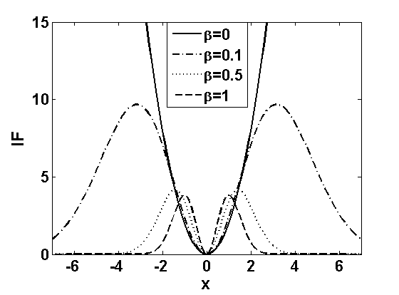
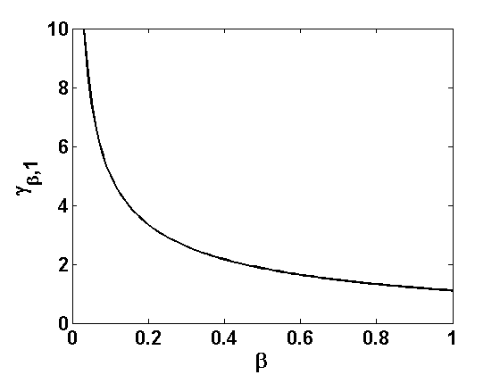
(a) Influence function
Refer to caption
(b) Gross error sensitivity
Figure 1: Second order influence function of the proposed Wald-type test statistics and corresponding gross error sensitivity $\gamma_{\beta,1}$ under contamination only in first sample for testing equality of two normal means as in Example 2.2 with known common $\sigma^{2}=1$
Example 2.2 (Continuation of Example 2.1)

Let us again consider the previous example on testing two normal means as in Example 2.1. We have seen that the proposed Wald-type tests are consistent for all $\beta\geq 0$ but their power against contiguous alternatives decreases slightly as $\beta$ increases. Now let us verify the claimed robustness of these tests.

Clearly, the first order IFs of the test statistics will always be zero. For contamination only in the first sample, the second order IF of the test statistic $T_{\beta}$ at the null hypothesis in (2) has a simpler form given by

$$IF_{2}^{(1)}(x;T_{\beta},F_{{{\theta}}_{1}},F_{{{\theta}}_{1}})=\frac{2}{\sigma^{2}}\left(1+2\beta\right)^{3/2}(x-{{\theta}}_{1})^{2}e^{-\frac{\beta(x-{{\theta}}_{1})^{2}}{\sigma^{2}}}.$$

Figure 1a presents the plot of this second order IF for different values of $\beta\in[0,1]$. It is evident from the figure that the second order IF is unbounded at $\beta=0$ implying the non-robustness of the classical Wald test statistic; but it is bounded for all $\beta>0$ implying the robustness of our proposals. Further, Figure 1b presents the plot of the maximum possible influence of infinitesimal contamination on the test statistics, known as the β€œgross error sensitivity”, computed as

$$\gamma_{\beta,1}=\sup_{x}\left|\left|IF_{2}^{(1)}(x;T_{\beta},F_{{{\theta}}_{1}},F_{{{\theta}}_{1}})\right|\right|=\frac{2}{\sigma^{3}\sqrt{\beta}}\left(1+\frac{\beta}{1+\beta}\right)e^{-\frac{\sqrt{\beta}}{\sigma}}.$$

It clearly shows that the robustness of our proposed test statistics increases as $\beta$ increases (since $\gamma_{\beta,1}$ decreases). Thus, just like the trade-off between efficiency and robustness of MDPDE, the parameter $\beta$ again controls the trade-off between asymptotic contiguous power and robustness for the proposed MDPDE based test statistics.

Similar inferences can also be drawn for contamination only in the second sample.

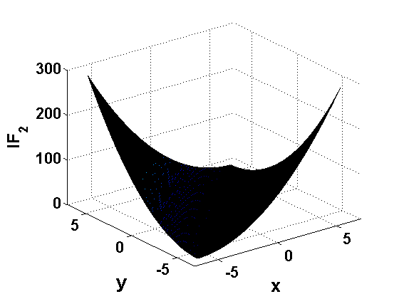
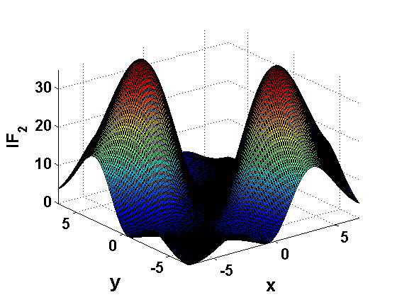
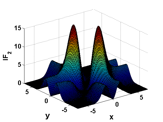
Next consider the case when there is contamination in both the samples. In this case, the second order IF is given by

$$IF_{2}(x,y;T_{\beta},F_{{{\theta}}_{1}},F_{{{\theta}}_{1}})=\frac{2}{\sigma^{2}}\left(1+2\beta\right)^{3/2}\left[(x-{{\theta}}_{1})e^{-\frac{\beta(x-{{\theta}}_{1})^{2}}{2\sigma^{2}}}-(y-{{\theta}}_{1})e^{-\frac{\beta(y-{{\theta}}_{1})^{2}}{2\sigma^{2}}}\right]^{2}.$$

The plot of $IF_{2}(x,y;T_{\beta},F_{{{\theta}}_{1}},F_{{{\theta}}_{1}})$ have been presented in Figure 2, which clearly show the robust nature of our proposals at $\beta>0$ and the non-robust nature of the classical Wald test (at $\beta=0$) unless $x=y$. By looking at the maximum possible influence in this case, we can again see that, even under contamination in both the samples, the robustness of our proposed Wald-type test statistics increases as $\beta$ increases.

Refer to caption
(a) $\beta=0$
Refer to caption
(b) $\beta=0.1$
Refer to caption
(c) $\beta=0.5$
Figure 2: Second order influence function of the proposed Wald-type test statistics under contamination in both the samples for testing equality of two normal means as in Example 2.2 with known common $\sigma^{2}=1$

2.3 Power and Level Influence Functions

The robustness of a test statistic, although necessary, may not be sufficient in all the cases since the performance of any test is finally measured through its level and power. In this section, we consider the effect of contamination on the asymptotic power and level of the proposed Wald-type tests. Due to consistency, the asymptotic power against any fixed alternative will be one. So, we again consider the contiguous alternatives $H_{1,m,n}$ given by (12) along with contamination over these alternatives. Following Hampel et al.Β (1986), the effect of contaminations should tend to zero, as the alternatives tend to the null (i.e., ${\boldsymbol{\theta}}_{1,n}\rightarrow{\boldsymbol{\theta}}_{0}$ and ${\boldsymbol{\theta}}_{2,m}\rightarrow{\boldsymbol{\theta}}_{0}$ as $m,n\rightarrow\infty$) at the same rate to avoid confusion between the neighborhoods of the two hypotheses (also see Huber-Carol (1970), Heritier and Ronchetti (1994), Toma and Broniatowski (2011), Ghosh et al. (2015, 2016) for some one sample applications). Further, in case of the present two sample problem, the contamination can be in any one sample or in both the samples. When the contamination is only in the first sample, we consider the corresponding contamination distribution for the first population as

$$F_{1,n,\varepsilon,x}^{L}=\left(1-\frac{\varepsilon}{\sqrt{n}}\right)F_{{\boldsymbol{\theta}}_{0}}+\frac{\varepsilon}{\sqrt{n}}\wedge_{x}~{}~{}~{}~{}F_{1,n,\varepsilon,x}^{P}=\left(1-\frac{\varepsilon}{\sqrt{n}}\right)F_{{\boldsymbol{\theta}}_{1,n}}+\frac{\varepsilon}{\sqrt{n}}\wedge_{x},$$

for the level and power calculations respectively along with the usual uncontaminated distributions for the second population. 
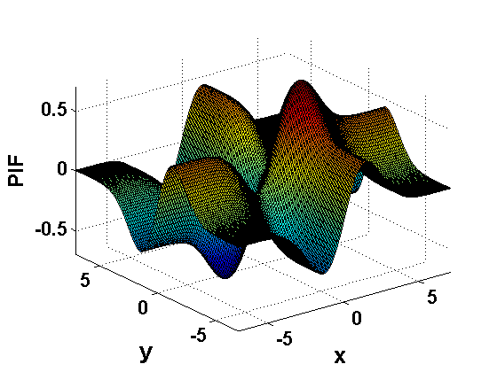
Then the corresponding level influence function (LIF) and the power influence function (PIF) at the null 𝜽1=𝜽2=𝜽0subscript𝜽1subscript𝜽2subscript𝜽0{\boldsymbol{\theta}}_{1}={\boldsymbol{\theta}}_{2}={\boldsymbol{\theta}}_{0} are given by

$$LIF^{(1)}(x;T_{\beta},F_{{\boldsymbol{\theta}}_{0}})=\lim_{m,n\rightarrow\infty}~{}\frac{\partial}{\partial\varepsilon}P_{(F_{1,n,\varepsilon,x}^{L},F_{{\boldsymbol{\theta}}_{0}})}(T_{m,n}^{(\beta)}>\chi_{p,\alpha}^{2})\big{|}_{\varepsilon=0},~{}$$
$$PIF^{(1)}(x;T_{\beta},F_{{\boldsymbol{\theta}}_{0}})=\lim_{m,n\rightarrow\infty}~{}\frac{\partial}{\partial\varepsilon}P_{(F_{1,n,\varepsilon,x}^{P},F_{{\boldsymbol{\theta}}_{2,m}})}(T_{m,n}^{(\beta)}>\chi_{p,\alpha}^{2})\big{|}_{\varepsilon=0}.$$

Similarly, when contamination is assumed to be only in the second sample, then we take the uncontaminated distributions for the first population and the contaminated distribution for the second population as

$$F_{2,m,\varepsilon,y}^{L}=\left(1-\frac{\varepsilon}{\sqrt{m}}\right)F_{{\boldsymbol{\theta}}_{0}}+\frac{\varepsilon}{\sqrt{m}}\wedge_{y}~{}~{}~{}~{}F_{2,m,\varepsilon,y}^{P}=\left(1-\frac{\varepsilon}{\sqrt{m}}\right)F_{{\boldsymbol{\theta}}_{2,m}}+\frac{\varepsilon}{\sqrt{m}}\wedge_{y},$$

for the level and power calculations respectively. Corresponding LIF and PIF at the null ${\boldsymbol{\theta}}_{1}={\boldsymbol{\theta}}_{2}={\boldsymbol{\theta}}_{0}$ are given by

$$LIF^{(2)}(y;T_{\beta},F_{{\boldsymbol{\theta}}_{0}})=\lim_{m,n\rightarrow\infty}~{}\frac{\partial}{\partial\varepsilon}P_{(F_{{\boldsymbol{\theta}}_{0}},F_{2,m,\varepsilon,y}^{L})}(T_{m,n}^{(\beta)}>\chi_{p,\alpha}^{2})\big{|}_{\varepsilon=0},~{}$$
$$PIF^{(2)}(y;T_{\beta},F_{{\boldsymbol{\theta}}_{0}})=\lim_{m,n\rightarrow\infty}~{}\frac{\partial}{\partial\varepsilon}P_{(F_{{\boldsymbol{\theta}}_{1,n}},F_{2,m,\varepsilon,y}^{P})}(T_{m,n}^{(\beta)}>\chi_{p,\alpha}^{2})\big{|}_{\varepsilon=0}.$$

Finally, while considering contamination in both the samples with above contaminated distributions, we define the corresponding LIF and PIF as

$$LIF(x,y;T_{\beta},F_{{\boldsymbol{\theta}}_{0}})=\lim_{m,n\rightarrow\infty}~{}\frac{\partial}{\partial\varepsilon}P_{(F_{1,n,\varepsilon,x}^{L},F_{2,m,\varepsilon,y}^{L})}(T_{m,n}^{(\beta)}>\chi_{p,\alpha}^{2})\big{|}_{\varepsilon=0},~{}$$
$$PIF(x,y;T_{\beta},F_{{\boldsymbol{\theta}}_{0}})=\lim_{m,n\rightarrow\infty}~{}\frac{\partial}{\partial\varepsilon}P_{(F_{1,n,\varepsilon,x}^{P},F_{2,m,\varepsilon,y}^{P})}(T_{m,n}^{(\beta)}>\chi_{p,\alpha}^{2})\big{|}_{\varepsilon=0}.$$

First let us derive the asymptotic distribution of the proposed Wald-type test statistics $T_{m,n}^{(\beta)}$ under the contaminated distributions. Let us define $\widetilde{{\boldsymbol{\Delta}}}_{i}={\boldsymbol{\Delta}}_{i}+\varepsilon\mathcal{IF}(x_{i};\boldsymbol{U}_{\beta},F_{{\boldsymbol{\theta}}_{0}})$ for $i=1,2$ with $x_{1}=x$ and $x_{2}=y$. Then we have the following theorem.

Theorem 2.6

Suppose the model density satisfies the Lehmann and Basu et al.Β conditions and Assumption (A) holds. Then the asymptotic distribution of $T_{m,n}^{(\beta)}$ under any contaminated contiguous alternative distributions $(D_{1},D_{2})$ is $\chi_{p}^{2}\left(\lambda\right)$ where $\lambda$ is the parameter of non-centrality given by $\lambda=\widetilde{\boldsymbol{W}}_{\varepsilon}^{T}{\boldsymbol{\Sigma}}_{\beta}({\boldsymbol{\theta}}_{0})^{-1}\widetilde{\boldsymbol{W}}_{\varepsilon}$, where

$\displaystyle\begin{array}[]{r l l}\widetilde{\boldsymbol{W}}_{\varepsilon}=&\boldsymbol{W}\left(\widetilde{{\boldsymbol{\Delta}}}_{1},{{\boldsymbol{\Delta}}}_{2}\right),&\mbox{if }~{}(D_{1},D_{2})=(F_{1,n,\varepsilon,x}^{P},F_{{\boldsymbol{\theta}}_{2,m}}),\\ =&\boldsymbol{W}\left({{\boldsymbol{\Delta}}}_{1},\widetilde{{\boldsymbol{\Delta}}}_{2}\right),&\mbox{if }~{}(D_{1},D_{2})=(F_{{\boldsymbol{\theta}}_{1,n}},F_{2,m,\varepsilon,y}^{P}),\\ =&\boldsymbol{W}\left(\widetilde{{\boldsymbol{\Delta}}}_{1},\widetilde{{\boldsymbol{\Delta}}}_{2}\right),&\mbox{if }~{}(D_{1},D_{2})=(F_{1,n,\varepsilon,x}^{P},F_{2,m,\varepsilon,y}^{P}).\end{array}$ (17)

From the above theorem, we get the asymptotic power of the proposed Wald-type tests under the contaminated contiguous alternatives as

$$\pi_{\beta}({\boldsymbol{\Delta}}_{1},{\boldsymbol{\Delta}}_{2};\varepsilon)=P_{(D_{1},D_{2})}\left(T_{m,n}^{(\beta)}>\chi^{2}_{p,\alpha}\right)=1-F_{\chi_{p}^{2}\left(\widetilde{\boldsymbol{W}}_{\varepsilon}^{T}{\boldsymbol{\Sigma}}_{\beta}({\boldsymbol{\theta}}_{0})^{-1}\widetilde{\boldsymbol{W}}_{\varepsilon}\right)}(\chi^{2}_{p,\alpha}).$$

Using infinite series expansion of a non-central chi-square distribution function (Kotz etΒ al., 1967), we get

$\displaystyle\pi_{\beta}({\boldsymbol{\Delta}}_{1},{\boldsymbol{\Delta}}_{2};\varepsilon)$ $\displaystyle=$ $\displaystyle\sum_{v=0}^{\infty}C_{v}\left(\widetilde{\boldsymbol{W}}_{\varepsilon},{\boldsymbol{\Sigma}}_{\beta}({\boldsymbol{\theta}}_{0})^{-1}\right)P\left(\chi^{2}_{p+2v}>\chi^{2}_{p,\alpha}\right),$
where $\displaystyle C_{v}(\boldsymbol{t},\boldsymbol{A})=\frac{(\boldsymbol{t}^{T}\boldsymbol{A}\boldsymbol{t})^{v}}{v!2^{v}}e^{-\frac{1}{2}\boldsymbol{t}^{T}\boldsymbol{A}\boldsymbol{t}}.~{}~{}~{}~{}~{}~{}~{}~{}~{}~{}~{}~{}~{}~{}~{}~{}~{}~{}~{}~{}~{}~{}~{}~{}~{}~{}~{}~{}~{}~{}~{}~{}~{}~{}~{}~{}~{}~{}~{}~{}~{}~{}~{}~{}~{}~{}~{}~{}~{}~{}$

In particular, substituting $\varepsilon=0$ in the above theorem, we get back Theorem 2.5 on the asymptotic contiguous power of our tests and hence expression (13) can be written as

$$\pi_{\beta}({\boldsymbol{\Delta}}_{1},{\boldsymbol{\Delta}}_{2})=\pi_{\beta}({\boldsymbol{\Delta}}_{1},{\boldsymbol{\Delta}}_{2};\boldsymbol{0}_{p})=\sum_{v=0}^{\infty}C_{v}\left(\boldsymbol{W}({\boldsymbol{\Delta}}_{1},\boldsymbol{\Delta}_{2}),{\boldsymbol{\Sigma}}_{\beta}({\boldsymbol{\theta}}_{0})^{-1}\right)P\left(\chi^{2}_{p+2v}>\chi^{2}_{p,\alpha}\right).$$

Further, substituting ${\boldsymbol{\Delta}}_{1}={\boldsymbol{\Delta}}_{2}=\boldsymbol{0}_{p}$, we get the asymptotic level of our Wald-type tests under the contamination as $\alpha_{\varepsilon}=\pi_{\beta}(\boldsymbol{0},\boldsymbol{0};\varepsilon)$.

Now we can define the power influence functions of our proposed tests which is nothing but $\left.\frac{\partial}{\partial\varepsilon}\pi_{\beta}({\boldsymbol{\Delta}}_{1},{\boldsymbol{\Delta}}_{2};\varepsilon)\right|_{\varepsilon=0}$ under standard regularity conditions. Using the infinite series expression of a non-central chi-square distribution function, we can derive an explicit form of the PIFs as presented in the following theorem.

Theorem 2.7

Suppose the model density satisfies the Lehmann and Basu et al.Β conditions, and Assumption (A) holds. Then the power influence functions of our proposed Wald-type tests are given by

$\displaystyle PIF^{(1)}(x;T_{\beta},F_{{\boldsymbol{\theta}}_{0}})$ $\displaystyle=$ $\displaystyle\sqrt{\omega}K_{p}^{*}\left(\delta_{\beta}\right)\boldsymbol{W}({\boldsymbol{\Delta}}_{1},\boldsymbol{\Delta}_{2})^{T}{\boldsymbol{\Sigma}}_{\beta}({\boldsymbol{\theta}}_{0})^{-1}\mathcal{IF}(x;\boldsymbol{U}_{\beta},F_{{\boldsymbol{\theta}}_{0}}),$
$\displaystyle PIF^{(2)}(y;T_{\beta},F_{{\boldsymbol{\theta}}_{0}})$ $\displaystyle=$ $\displaystyle\sqrt{1-\omega}K_{p}^{*}\left(\delta_{\beta}\right)\boldsymbol{W}({\boldsymbol{\Delta}}_{1},\boldsymbol{\Delta}_{2})^{T}{\boldsymbol{\Sigma}}_{\beta}({\boldsymbol{\theta}}_{0})^{-1}\mathcal{IF}(y;\boldsymbol{U}_{\beta},F_{{\boldsymbol{\theta}}_{0}}),$
$\displaystyle PIF(x,y;T_{\beta},F_{{\boldsymbol{\theta}}_{0}})$ $\displaystyle=$ $\displaystyle K_{p}^{*}\left(\delta_{\beta}\right)\boldsymbol{W}({\boldsymbol{\Delta}}_{1},\boldsymbol{\Delta}_{2})^{T}{\boldsymbol{\Sigma}}_{\beta}({\boldsymbol{\theta}}_{0})^{-1}\boldsymbol{W}\left(\mathcal{IF}(x;\boldsymbol{U}_{\beta},F_{{\boldsymbol{\theta}}_{0}}),\mathcal{IF}(x;\boldsymbol{U}_{\beta},F_{{\boldsymbol{\theta}}_{0}})\right),$

where $\delta_{\beta}$ and $\boldsymbol{W}({\boldsymbol{\Delta}}_{1},\boldsymbol{\Delta}_{2})$ are as defined in Theorem 2.5 and

$$K_{p}^{*}(s)=e^{-\frac{s}{2}}\sum_{v=0}^{\infty}\frac{s^{v-1}}{v!2^{v}}\left(2v-s\right)P\left(\chi^{2}_{p+2v}>\chi^{2}_{p,\alpha}\right).$$

Note that the PIFs are also a function of the influence function of the MDPDE used and hence they are bounded whenever $\beta>0$. Thus the proposed tests will be robust for all $\beta>0$. However, at $\beta=0$, these PIFs will be unbounded (unless there is contamination at the same points $x=y$ in both the samples) which proves the non-robust nature of the classical Wald test.

Note that, although there is no direct relationship between the IF of test statistics with the corresponding PIF in general, in this present case they are seen to be related indirectly via the IF of the MDPDE. So, using a robust MDPDE with $\beta>0$ in the proposed Wald-type tests will make both the test statistics and its asymptotic power robust under infinitesimal contamination.

Finally, we can find the level influence function of the proposed Wald-type tests either starting from $\alpha_{\varepsilon}$ and following the same steps as in the case of PIFs or just by substituting ${\boldsymbol{\Delta}}_{1}={\boldsymbol{\Delta}}_{2}=\boldsymbol{0}$ in the expression of the PIFs given in Theorem 2.7. In either case, since $\boldsymbol{W}({\boldsymbol{0}},{\boldsymbol{0}})=\boldsymbol{0}$, it turns out that

$$LIF^{(1)}(x;T_{\beta},F_{{\boldsymbol{\theta}}_{0}})=0,~{}~{}~{}LIF^{(2)}(y;T_{\beta},F_{{\boldsymbol{\theta}}_{0}})=0,~{}~{}~{}LIF(x,y;T_{\beta},F_{{\boldsymbol{\theta}}_{0}})=0,$$ (18)

provided the corresponding IF of $\boldsymbol{U}_{\beta}$ is bounded, which is true at $\beta>0$. Hence the asymptotic level of our Wald-type tests is always stable with respect infinitesimal contamination. This fact was also expected as we are using the asymptotic critical values for testing.

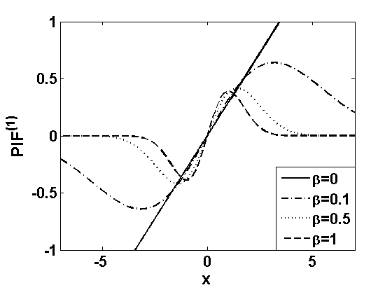
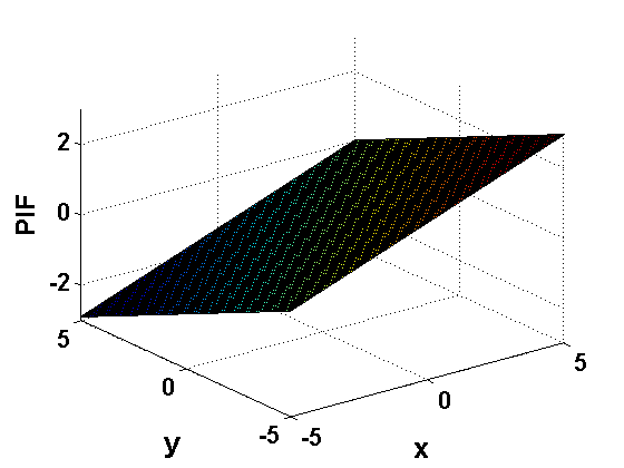
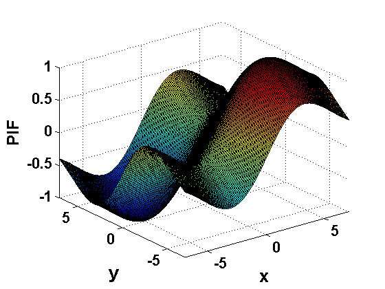
Example 2.3 (Continuation of Examples 2.1 and 2.2)

Let us again consider the problem of testing for normal means as in Examples 2.1 and 2.2. As seen above, the level influence function is always zero implying the level robustness of our proposed Wald-type test for all $\beta>0$. Next, to study the power robustness, we compute the functions $PIF^{(1)}(x;T_{\beta},F_{{{\theta}}_{0}})$ and $PIF(x,y;T_{\beta},F_{{{\theta}}_{0}})$ numerically for different values of $\beta$ with $\theta_{0}=0$ and plot them over the contamination points $x$ and $y$ in Figure 3. $PIF^{(2)}(y;T_{\beta},F_{{{\theta}}_{0}})$ has the same nature as $PIF^{(1)}(x;T_{\beta},F_{{{\theta}}_{0}})$. The figures clearly show the robustness of the proposed Wald-type tests with $\beta>0$, where the robustness increases (i.e., maximum possible PIF decreases) as $\beta$ increases. Further, all the PIFs at $\beta=0$ are unbounded implying the non-robust nature of the classical Wald test.

Refer to caption
(a) Contamination in only first samples
Refer to caption
(b) Contamination in both samples, $\beta=0$
Refer to caption
(c) Contamination in both samples, $\beta=0.1$
Refer to caption
(d) Contamination in both samples, $\beta=0.5$
Figure 3: Power influence functions of the proposed Wald-type test statistics at 95% level for testing equality of two normal means as in Example 2.3 with known common $\sigma^{2}=1$, $W(\Delta_{1},\Delta_{2})=2$ and $\omega=0.5$ ($n=m$).

3 General Composite Hypotheses with Two Samples

In the previous section, we have considered the simplest two sample problem which tests for equality of all the model parameters. However, in practice, we need to test many different complicated hypotheses which cannot be solved just by considering the Wald-type test statistic $T_{m,n}^{(\beta)}$ defined in the previous section. For example, in many real life problems, we are only interested in a proper subset of the parameters ignoring the rest as nuisance parameters; example includes popular mean test taking variance parameter unknown and nuisance. Further, in case of testing for multiplicative heteroscedasticity of two samples, we have to test if the ratio of variance parameters equals a pre-specified limit with means being unknown and nuisance. Neither of them belongs to the problem considered in the previous section.

In this section, we will consider a general class of hypotheses involving two independent samples, which would include most of the above real life testing problems. Suppose ${\boldsymbol{\psi}}({\boldsymbol{\theta}}_{1},{\boldsymbol{\theta}}_{2})$ denote a general function from $\mathbb{R}^{p}\times\mathbb{R}^{p}$ to $\mathbb{R}^{r}$. Then, considering the set-up of the previous section, we want to develop a family of robust tests for the general class of hypothesis given by

H0:𝝍​(𝜽1,𝜽2)=𝟎r​againstH1:𝝍​(𝜽1,𝜽2)β‰ πŸŽr.:subscript𝐻0𝝍subscript𝜽1subscript𝜽2subscript0π‘Ÿagainstsubscript𝐻1:𝝍subscript𝜽1subscript𝜽2subscript0π‘ŸH_{0}:{\boldsymbol{\psi}}({\boldsymbol{\theta}}_{1},{\boldsymbol{\theta}}_{2})=\boldsymbol{0}_{r}~{}~{}~{}\mbox{against}~{}~{}~{}~{}H_{1}:{\boldsymbol{\psi}}({\boldsymbol{\theta}}_{1},{\boldsymbol{\theta}}_{2})\neq\boldsymbol{0}_{r}. (19)

In particular, the problem of testing normal mean with unknown variance can be seen as a particular case of the above general set-up with ${\boldsymbol{\psi}}((\mu_{1},\sigma_{1}^{2}),(\mu_{2},\sigma_{2}^{2}))=\mu_{1}-\mu_{2}$. Further, to test for multiplicative heteroscedasticity, we can take ${\boldsymbol{\psi}}((\mu_{1},\sigma_{1}^{2}),(\mu_{2},\sigma_{2}^{2}))=\frac{\sigma_{1}^{2}}{\sigma_{2}^{2}}-C_{0}$ for some known constant $C_{0}$ and apply the above general set-up. It is interesting to note that, this general class of hypotheses in (19) also contains the simple hypothesis in (2) as its special case with ${\boldsymbol{\psi}}({\boldsymbol{\theta}}_{1},{\boldsymbol{\theta}}_{2})={\boldsymbol{\theta}}_{1}-{\boldsymbol{\theta}}_{2}$.

Now, to define a robust Wald-type test statistics for this general set-up, we again consider the MDPDEs of ${\boldsymbol{\theta}}_{1}$ and ${\boldsymbol{\theta}}_{2}$ with tuning parameter $\beta$ as given by ${}^{(1)}\widehat{{\boldsymbol{\theta}}}_{\beta}$ and ${}^{(2)}\widehat{{\boldsymbol{\theta}}}_{\beta}$ based on the individual samples separately. Note that, whenever $H_{0}$ is true, we should have ${\boldsymbol{\psi}}(^{(1)}\widehat{{\boldsymbol{\theta}}}_{\beta},^{(2)}\widehat{{\boldsymbol{\theta}}}_{\beta})\approx\boldsymbol{0}_{r}$ in large sample and so its observed value provide the indication of any departure from the null hypothesis. Using its asymptotic variance-covariance matrix as a normalizing factor, we define the corresponding Wald-type test statistic as

$$\widetilde{T_{m,n}^{(\beta)}}=\frac{nm}{n+m}~{}{\boldsymbol{\psi}}\left({}^{(1)}\widehat{{\boldsymbol{\theta}}}_{\beta},^{(2)}\widehat{{\boldsymbol{\theta}}}_{\beta}\right)^{T}\widetilde{{\boldsymbol{\Sigma}}_{\beta}}(^{(1)}\widehat{{\boldsymbol{\theta}}}_{\beta},^{(2)}\widehat{{\boldsymbol{\theta}}}_{\beta})^{-1}{\boldsymbol{\psi}}\left({}^{(1)}\widehat{{\boldsymbol{\theta}}}_{\beta},^{(2)}\widehat{{\boldsymbol{\theta}}}_{\beta}\right),$$ (20)

where $\widetilde{{\boldsymbol{\Sigma}}_{\beta}}({\boldsymbol{\theta}}_{1},{\boldsymbol{\theta}}_{2})=\omega{\boldsymbol{\Psi}}_{1}({\boldsymbol{\theta}}_{1},{\boldsymbol{\theta}}_{2})^{T}{\boldsymbol{\Sigma}}_{\beta}({\boldsymbol{\theta}}_{1}){\boldsymbol{\Psi}}_{1}({\boldsymbol{\theta}}_{1},{\boldsymbol{\theta}}_{2})+(1-\omega){\boldsymbol{\Psi}}_{2}({\boldsymbol{\theta}}_{1},{\boldsymbol{\theta}}_{2})^{T}{\boldsymbol{\Sigma}}_{\beta}({\boldsymbol{\theta}}_{2}){\boldsymbol{\Psi}}_{2}({\boldsymbol{\theta}}_{1},{\boldsymbol{\theta}}_{2})$ with

$${\boldsymbol{\Psi}}_{i}({\boldsymbol{\theta}}_{1},{\boldsymbol{\theta}}_{2})=\frac{\partial}{\partial{\boldsymbol{\theta}}_{i}}{\boldsymbol{\psi}}({\boldsymbol{\theta}}_{1},{\boldsymbol{\theta}}_{2})^{T},~{}~{}~{}~{}i=1,2.$$

Note that, at $\beta=0$, the Wald-type test statistics $\widetilde{T_{m,n}^{(0)}}$ is again nothing but the classical Wald test statistics for the general hypothesis (19) and hence our proposal is indeed a generalization of the classical Wald test.

Interestingly, although the general hypothesis contains the hypothesis (2) as its special case, the Wald-type test statistics $\widetilde{T_{m,n}^{(\beta)}}$ with ${\boldsymbol{\psi}}({\boldsymbol{\theta}}_{1},{\boldsymbol{\theta}}_{2})={\boldsymbol{\theta}}_{1}-{\boldsymbol{\theta}}_{2}$ is not the same as the Wald-type test statistics $T_{m,n}^{(\beta)}$ considered in the previous section. However, whenever $\boldsymbol{\Sigma}_{\beta}({\boldsymbol{\theta}})$ is linear in the parameters, these two Wald-type test statistics coincide asymptotically with probability tending to one. In this section, we present the properties of the statistics $\widetilde{T_{m,n}^{(\beta)}}$ with general ${\boldsymbol{\psi}}$-function satisfying the following assumption.

Assumption (B):

  • β€’

    𝚿i​(𝜽1,𝜽2)subscriptπšΏπ‘–subscript𝜽1subscript𝜽2{\boldsymbol{\Psi}}_{i}({\boldsymbol{\theta}}_{1},{\boldsymbol{\theta}}_{2}), $i=1,2$, exist, have rank $r$ and are continuous with respect to its arguments.

3.1 Asymptotic Properties

We again start with the asymptotic null distribution of the proposed Wald-type test statistics $\widetilde{T_{m,n}^{(\beta)}}$ in order to obtain the required critical values for the test.

Theorem 3.1

Suppose the model density satisfies the Lehmann and Basu et al.Β conditions and Assumptions (A) and (B) hold. Then, under the null hypothesis in (19), $\widetilde{T_{m,n}^{(\beta)}}$ asymptotically follows a $\chi_{r}^{2}$ distribution.

Therefore, the level-$\alpha$ critical region for the proposed test based on $\widetilde{T_{m,n}^{(\beta)}}$ for testing (19) is given by

$$\widetilde{T_{m,n}^{(\beta)}}>\chi^{2}_{r,\alpha}.$$

Next, in order to consider an approximation to the asymptotic power for this general test based on $\widetilde{T_{m,n}^{(\beta)}}$, we are going to use the following function

$$\widetilde{l^{*}}({\boldsymbol{\theta}}_{1},{\boldsymbol{\theta}}_{2})={\boldsymbol{\psi}}({\boldsymbol{\theta}}_{1},{\boldsymbol{\theta}}_{2})^{T}\widetilde{{\boldsymbol{\Sigma}}_{\beta}}({\boldsymbol{\theta}}_{1},{\boldsymbol{\theta}}_{2})^{-1}{\boldsymbol{\psi}}({\boldsymbol{\theta}}_{1},{\boldsymbol{\theta}}_{2}).$$
Theorem 3.2

Suppose the model density satisfies the Lehmann and Basu et al.Β conditions and Assumptions (A)-(B) hold. Then, whenever 𝛙​(𝛉1,𝛉2)β‰ πŸŽr𝛙subscript𝛉1subscript𝛉2subscript0π‘Ÿ{\boldsymbol{\psi}}({\boldsymbol{\theta}}_{1},{\boldsymbol{\theta}}_{2})\neq\boldsymbol{0}_{r}, we have

$\displaystyle\sqrt{\frac{mn}{m+n}}\left[\widetilde{l^{*}}(^{(1)}\widehat{{\boldsymbol{\theta}}}_{\beta},^{(2)}\widehat{{\boldsymbol{\theta}}}_{\beta})-\widetilde{l^{*}}({\boldsymbol{\theta}}_{1},{\boldsymbol{\theta}}_{2})\right]\underset{m,n\rightarrow\infty}{\overset{\mathcal{L}}{\longrightarrow}}N\left(0,4\widetilde{l^{*}}({\boldsymbol{\theta}}_{1},{\boldsymbol{\theta}}_{2})\right),~{}\mbox{ as }~{}m,n\rightarrow\infty.$ (21)

Note that, from the above theorem, we can easily obtain an approximation to the power function of the proposed level-$\alpha$ Wald-type tests based on $\widetilde{T_{m,n}^{(\beta)}}$ as

$\displaystyle\widetilde{\pi_{m,n,\alpha}}^{(\beta)}({\boldsymbol{\theta}}_{1},{\boldsymbol{\theta}}_{2})=P\left(\widetilde{T_{m,n}^{(\beta)}}>\chi_{r,\alpha}^{2}\right)=1-\Phi_{n}\left(\frac{\sqrt{\frac{n+m}{nm}}}{2\sqrt{\widetilde{l^{*}}({\boldsymbol{\theta}}_{1},{\boldsymbol{\theta}}_{2})}}\left[\chi_{r,\alpha}^{2}-\frac{nm}{n+m}\widetilde{l^{*}}({\boldsymbol{\theta}}_{1},{\boldsymbol{\theta}}_{2})\right]\right),$

for a sequence of distributions $\Phi_{n}(\cdot)$ tending uniformly to the standard normal distribution $\Phi(\cdot)$, whenever 𝝍​(𝜽1,𝜽2)β‰ πŸŽr𝝍subscript𝜽1subscript𝜽2subscript0π‘Ÿ{\boldsymbol{\psi}}({\boldsymbol{\theta}}_{1},{\boldsymbol{\theta}}_{2})\neq\boldsymbol{0}_{r}. In such cases, it can be easily checked that $\widetilde{\pi_{m,n,\alpha}}^{(\beta)}({\boldsymbol{\theta}}_{1},{\boldsymbol{\theta}}_{2})\rightarrow 1$ as $m,n\rightarrow\infty$. This proves the consistency of our proposed tests.

Corollary 3.3

Under the assumptions of Theorem 3.2, the proposed Wald-type tests based on $\widetilde{T_{m,n}^{(\beta)}}$ are consistent.

Now, let us study the performance of the proposed general two-sample Wald-type tests under the contiguous alternative hypotheses. As discussed in the previous section, there could be different choices for the contiguous alternative hypotheses for any general null hypothesis. Here, following the similar idea as in the alternatives in (12), we consider the general form of the contiguous alternatives given by

$$H_{1,n,m}:{\boldsymbol{\theta}}_{1}={\boldsymbol{\theta}}_{1,n}={\boldsymbol{\theta}}_{10}+n^{-\frac{1}{2}}{\boldsymbol{\Delta}}_{1},~{}~{}{\boldsymbol{\theta}}_{2}={\boldsymbol{\theta}}_{2,m}={\boldsymbol{\theta}}_{20}+m^{-\frac{1}{2}}{\boldsymbol{\Delta}}_{2},~{}~{}~{}~{}~{}~{}({\boldsymbol{\Delta}}_{1},{\boldsymbol{\Delta}}_{2})\in\mathbb{R}^{p}\times\mathbb{R}^{p}-\{(\boldsymbol{0}_{p},\boldsymbol{0}_{p})\},$$ (22)

for some fixed $\left({\boldsymbol{\theta}}_{10},{\boldsymbol{\theta}}_{20}\right)\in\Theta_{0}=\{\left({\boldsymbol{\theta}}_{1},{\boldsymbol{\theta}}_{2}\right)\in\Theta\times\Theta:\boldsymbol{\psi}({\boldsymbol{\theta}}_{1},{\boldsymbol{\theta}}_{2})=0\}$. The asymptotic distribution of $\widetilde{T_{m,n}^{(\beta)}}$ under these alternatives $H_{1,m,n}$ has been presented in the following theorem.

Theorem 3.4

Suppose the model density satisfies the Lehmann and Basu et al.Β conditions and Assumptions (A)-(B) hold. Then the asymptotic distribution of $\widetilde{T_{m,n}^{(\beta)}}$ under $H_{1,n,m}$ in (22) is $\chi^{2}_{r}(\widetilde{\delta_{\beta}})$, where

$$\widetilde{\delta_{\beta}}=\boldsymbol{W}_{\boldsymbol{\psi}}({\boldsymbol{\Delta}}_{1},{\boldsymbol{\Delta}}_{2})^{T}\widetilde{{\boldsymbol{\Sigma}}_{\beta}}({\boldsymbol{\theta}}_{1},{\boldsymbol{\theta}}_{2})^{-1}\boldsymbol{W}_{\boldsymbol{\psi}}({\boldsymbol{\Delta}}_{1},{\boldsymbol{\Delta}}_{2})$$

with $\boldsymbol{W}_{\boldsymbol{\psi}}({\boldsymbol{\Delta}}_{1},{\boldsymbol{\Delta}}_{2})=\left[\sqrt{\omega}{\boldsymbol{\Psi}}_{1}({\boldsymbol{\theta}}_{1},{\boldsymbol{\theta}}_{2})^{T}{\boldsymbol{\Delta}}_{1}+\sqrt{1-\omega}{\boldsymbol{\Psi}}_{2}({\boldsymbol{\theta}}_{1},{\boldsymbol{\theta}}_{2})^{T}{\boldsymbol{\Delta}}_{2}\right].$

The above theorem directly helps us to obtain the asymptotic power $\widetilde{\pi}_{\beta}({\boldsymbol{\Delta}}_{1},{\boldsymbol{\Delta}}_{2})$ of our general Wald-type tests based on $\widetilde{T_{m,n}^{(\beta)}}$ under the contiguous alternatives $H_{1,n,m}$ in (22) as

$$\widetilde{\pi}_{\beta}({\boldsymbol{\Delta}}_{1},{\boldsymbol{\Delta}}_{2})=1-F_{\chi^{2}_{r}(\widetilde{\delta_{\beta}})}(\chi^{2}_{r,\alpha}).$$

3.2 Robustness Properties

Let us now study the robustness properties of the proposed general two-sample Wald-type tests based on $\widetilde{T_{m,n}^{(\beta)}}$. We first consider the influence function of the Wald-type test statistics. Define the statistical functional corresponding to $\widetilde{T_{m,n}^{(\beta)}}$ ignoring the multiplier $\frac{nm}{n+m}$ as

$$\widetilde{T_{\beta}}(G_{1},G_{2})={\boldsymbol{\psi}}\left(\boldsymbol{U}_{\beta}(G_{1}),\boldsymbol{U}_{\beta}(G_{2})\right)^{T}\widetilde{{\boldsymbol{\Sigma}}_{\beta}}^{-1}({\boldsymbol{\theta}}_{1},{\boldsymbol{\theta}}_{2}){\boldsymbol{\psi}}\left(\boldsymbol{U}_{\beta}(G_{1}),\boldsymbol{U}_{\beta}(G_{2})\right),$$

where $\boldsymbol{U}_{\beta}$ is the corresponding MDPDE functional. Then, we can derive the first and second order influence functions of the Wald-type test statistics following the derivations similar to that of Section 2.2. So, here we will skip those derivations for brevity and present only the final results in the following theorem.

Theorem 3.5

Consider the notations of Section 2.2. Under the null hypothesis in (19) with $G_{1}=F_{{\boldsymbol{\theta}}_{10}}$, $G_{2}=F_{{\boldsymbol{\theta}}_{20}}$ and ${\boldsymbol{\psi}}({\boldsymbol{\theta}}_{10},{{\boldsymbol{\theta}}_{20}})=0$, the first and second order influence functions of our general two-sample Wald-type test statistics are given as follows:

  1. 1.

    For contamination only in the $i$-th sample ($i=1,2$) at the point $x_{i}$ ($x_{1}=x,x_{2}=y$)

    $\displaystyle IF^{(i)}(x_{i};\widetilde{T_{\beta}},F_{{\boldsymbol{\theta}}_{10}},F_{{\boldsymbol{\theta}}_{20}})$ $\displaystyle=$ $\displaystyle 0,$
    $\displaystyle IF^{(i)}_{2}(x_{i};\widetilde{T_{\beta}},F_{{\boldsymbol{\theta}}_{i0}},F_{{\boldsymbol{\theta}}_{20}})$ $\displaystyle=$ $\displaystyle 2\mathcal{IF}(x_{i};\boldsymbol{U}_{\beta},F_{{\boldsymbol{\theta}}_{10}})^{T}{\boldsymbol{\Psi}}_{i}({\boldsymbol{\theta}}_{10},{\boldsymbol{\theta}}_{20})^{T}\widetilde{{\boldsymbol{\Sigma}}_{\beta}}({\boldsymbol{\theta}}_{10},{\boldsymbol{\theta}}_{20})^{-1}{\boldsymbol{\Psi}}_{i}({\boldsymbol{\theta}}_{10},{\boldsymbol{\theta}}_{20})\mathcal{IF}(x_{i};\boldsymbol{U}_{\beta},{\boldsymbol{\theta}}_{i0}).$
  2. 2.

    For contamination in both the samples

    $\displaystyle IF(x,y;\widetilde{T_{\beta}},F_{{\boldsymbol{\theta}}_{10}},F_{{\boldsymbol{\theta}}_{20}})$ $\displaystyle=$ $\displaystyle 0$
    $\displaystyle IF_{2}(x,y;\widetilde{T_{\beta}},F_{{\boldsymbol{\theta}}_{10}},F_{{\boldsymbol{\theta}}_{20}})$ $\displaystyle=$ $\displaystyle 2\boldsymbol{Q}_{\beta}(x,y)^{T}\widetilde{{\boldsymbol{\Sigma}}_{\beta}}({\boldsymbol{\theta}}_{10},{\boldsymbol{\theta}}_{20})^{-1}\boldsymbol{Q}_{\beta}(x,y).$

    with $\boldsymbol{Q}_{\beta}(x,y)={\boldsymbol{\Psi}}_{1}({\boldsymbol{\theta}}_{10},{\boldsymbol{\theta}}_{20})^{T}\mathcal{IF}(x;\boldsymbol{U}_{\beta},F_{{\boldsymbol{\theta}}_{10}})+{\boldsymbol{\Psi}}_{2}({\boldsymbol{\theta}}_{10},{\boldsymbol{\theta}}_{20})^{T}\mathcal{IF}(y;\boldsymbol{U}_{\beta},F_{{\boldsymbol{\theta}}_{20}}).$

Clearly, as in the previous case of simple two sample problem in Section 2.2, here also the first order IF of the test statistics are always zero and hence non-informative about their robustness. However, their second order IFs are clearly bounded whenever the IF of the corresponding MDPDE is bounded which holds for all $\beta>0$. Thus, the proposed general two sample Wald-type tests with any $\beta>0$ yield robust solution under contamination in either of the samples or in both. Further, in case of contamination in both the samples, if the IF of the MDPDE is not bounded (at $\beta=0$), then also the corresponding second order IF can be bounded generating robust inference provided the term $\boldsymbol{Q}_{\beta}(x,y)$ is bounded. One example of such situation arises in case of the simpler problem of Section 2 under the choice $x=y$, because in that case ${\boldsymbol{\Psi}}_{1}({\boldsymbol{\theta}}_{10},{\boldsymbol{\theta}}_{20})=-{\boldsymbol{\Psi}}_{2}({\boldsymbol{\theta}}_{10},{\boldsymbol{\theta}}_{20})=\boldsymbol{I}_{p}$, the identity matrix of oder $p$, and hence $\boldsymbol{Q}_{\beta}(x,y)$ becomes identically zero.

Next, we consider the effect of contamination on the asymptotic power and level of the proposed general Wald-type tests based on $\widetilde{T_{m,n}^{(\beta)}}$. For this general case, we consider the contiguous alternatives $H_{1,m,n}$ as defined in (22) but now with the null baseline parameter values as $\boldsymbol{\theta}_{10}$ and $\boldsymbol{\theta}_{20}$ for the two samples respectively instead of the common $\boldsymbol{\theta}_{0}$ and define the level and power influence functions using the corresponding contaminated distributions as in Section 2.3. Following theorem presents the asymptotic distribution of the test statistics under the contiguous and contaminated distributions, where $\widetilde{\boldsymbol{\Delta}}_{i}$s ($i=1,2$) are as defined in Section 2.3.

Theorem 3.6

Suppose the model density satisfies the Lehmann and Basu et al.Β conditions and Assumptions (A)-(B) hold. Then, the asymptotic distribution of the general Wald-type test statistics $\widetilde{T_{m,n}^{(\beta)}}$ under any contaminated contiguous alternative distributions $(D_{1},D_{2})$ is non-central chi-square with $r$ degrees of freedom and non-centrality parameter $\widetilde{\boldsymbol{W}_{\varepsilon}^{*}}^{T}\widetilde{{\boldsymbol{\Sigma}}_{\beta}}({\boldsymbol{\theta}}_{1},{\boldsymbol{\theta}}_{2})^{-1}\widetilde{\boldsymbol{W}_{\varepsilon}^{*}}$, where

$$\begin{array}[]{r l l}\widetilde{\boldsymbol{W}_{\varepsilon}^{*}}=&\boldsymbol{W}_{\boldsymbol{\psi}}(\widetilde{{\boldsymbol{\Delta}}}_{1},{{\boldsymbol{\Delta}}}_{2}),&\mbox{if }~{}(D_{1},D_{2})=(F_{1,n,\varepsilon,x}^{P},F_{{\boldsymbol{\theta}}_{2,m}}),\\ =&\boldsymbol{W}_{\boldsymbol{\psi}}({{\boldsymbol{\Delta}}}_{1},\widetilde{{\boldsymbol{\Delta}}}_{2}),&\mbox{if }~{}(D_{1},D_{2})=(F_{{\boldsymbol{\theta}}_{1,n}},F_{2,m,\varepsilon,y}^{P}),\\ =&\boldsymbol{W}_{\boldsymbol{\psi}}(\widetilde{{\boldsymbol{\Delta}}}_{2},\widetilde{{\boldsymbol{\Delta}}}_{2}),&\mbox{if }~{}(D_{1},D_{2})=(F_{1,n,\varepsilon,x}^{P},F_{2,m,\varepsilon,y}^{P}).\end{array}$$

The above theorem can be used to get the asymptotic power of the proposed general two-sample Wald-type tests under the contiguous contaminated alternatives in terms of an infinite series following Section 2.3 (arguments after Theorem 2.6). This can be also simplified by substituting $\varepsilon=0$ or $\boldsymbol{\Delta}_{1}=\boldsymbol{\Delta}_{2}=\boldsymbol{0}_{p}$ to get asymptotic power under contiguous alternatives or the asymptotic level under contiguous contamination respectively. Further, the resulting infinite series expressions can now be used to obtain the power and level influence functions for this general case. Since the derivations are the same as that of Theorem 2.7, for brevity, we will only present the resulting expressions skipping the details in the following Theorem.

Theorem 3.7

Suppose the model density satisfies the Lehmann and Basu et al.Β conditions, and Assumptions (A)–(B) hold. Then we have the following results for the proposed Wald-type test functional $\widetilde{T}_{\beta}$ for testing the general two-sample hypothesis in (19).

  1. 1.

    The power influence functions are given by

    $\displaystyle PIF^{(1)}(x;\widetilde{{T}_{\beta}},F_{{\boldsymbol{\theta}}_{10}},F_{{\boldsymbol{\theta}}_{20}})$ $\displaystyle=$ $\displaystyle\sqrt{\omega}K_{r}^{*}\left(\widetilde{\delta_{\beta}}\right)\boldsymbol{W}_{\boldsymbol{\psi}}({\boldsymbol{\Delta}}_{1},\boldsymbol{\Delta}_{2})^{T}\widetilde{\boldsymbol{\Sigma}_{\beta}}({\boldsymbol{\theta}}_{0})^{-1}{\boldsymbol{\Psi}}_{1}({\boldsymbol{\theta}}_{10},{\boldsymbol{\theta}}_{20})^{T}\mathcal{IF}(x;\boldsymbol{U}_{\beta},F_{{\boldsymbol{\theta}}_{10}}),$
    $\displaystyle PIF^{(2)}(y;\widetilde{T_{\beta}},F_{{\boldsymbol{\theta}}_{10}},F_{{\boldsymbol{\theta}}_{20}})$ $\displaystyle=$ $\displaystyle\sqrt{1-\omega}K_{r}^{*}\left(\widetilde{\delta_{\beta}}\right)\boldsymbol{W}_{\boldsymbol{\psi}}({\boldsymbol{\Delta}}_{1},\boldsymbol{\Delta}_{2})^{T}\widetilde{\boldsymbol{\Sigma}_{\beta}}({\boldsymbol{\theta}}_{0})^{-1}{\boldsymbol{\Psi}}_{2}({\boldsymbol{\theta}}_{10},{\boldsymbol{\theta}}_{20})^{T}\mathcal{IF}(y;\boldsymbol{U}_{\beta},F_{{\boldsymbol{\theta}}_{20}}),$
    $\displaystyle PIF(x,y;\widetilde{T_{\beta}},F_{{\boldsymbol{\theta}}_{10}},F_{{\boldsymbol{\theta}}_{20}})$ $\displaystyle=$ $\displaystyle K_{r}^{*}\left(\widetilde{\delta_{\beta}}\right)\boldsymbol{W}_{\boldsymbol{\psi}}({\boldsymbol{\Delta}}_{1},\boldsymbol{\Delta}_{2})^{T}\widetilde{\boldsymbol{\Sigma}_{\beta}}({\boldsymbol{\theta}}_{0})^{-1}\boldsymbol{W}_{\boldsymbol{\psi}}\left(\mathcal{IF}(x;\boldsymbol{U}_{\beta},F_{{\boldsymbol{\theta}}_{10}}),\mathcal{IF}(y;\boldsymbol{U}_{\beta},F_{{\boldsymbol{\theta}}_{20}})\right),$

    where $\widetilde{\delta_{\beta}}$ and $\boldsymbol{W}_{\boldsymbol{\psi}}({\boldsymbol{\Delta}}_{1},\boldsymbol{\Delta}_{2})$ are as defined in Theorem 3.4 and Krβˆ—β€‹(s)superscriptsubscriptπΎπ‘Ÿπ‘ K_{r}^{*}(s) is as defined in Theorem 2.7.

  2. 2.

    Provided the IF of the MDPDE $\boldsymbol{U}_{\beta}$ is bounded, the level influence functions are given by

    $$LIF^{(1)}(x;\widetilde{T_{\beta}},F_{{\boldsymbol{\theta}}_{10}},F_{{\boldsymbol{\theta}}_{20}})=0,~{}~{}~{}LIF^{(2)}(y;\widetilde{T_{\beta}},F_{{\boldsymbol{\theta}}_{10}},F_{{\boldsymbol{\theta}}_{20}})=0,~{}~{}~{}LIF(x,y;\widetilde{T_{\beta}},F_{{\boldsymbol{\theta}}_{10}},F_{{\boldsymbol{\theta}}_{20}})=0.$$

Note that for the general two-sample hypothesis (19) also, the LIFs and the PIFs of our proposed test are bounded whenever the influence function of the MDPDE used is bounded which holds for all $\beta>0$. Thus, our proposal with $\beta>0$ is robust also for testing any general two-sample problem.

3.3 Special Case: Testing Partial Homogeneity with Nuisance Parameters

Let us consider a simplified and possibly the most common special case of the general hypothesis in (19), where we test for partial homogeneity of the two samples assuming some parameters to be nuisance. Mathematically, let us consider the partition of the parameters $\boldsymbol{{\boldsymbol{\theta}}}_{1}=\left({}^{\ast}\boldsymbol{{\boldsymbol{\theta}}}_{1}^{T},^{0}\boldsymbol{{\boldsymbol{\theta}}}_{1}^{T}\right)^{T}$ and $\boldsymbol{{\boldsymbol{\theta}}}_{2}=\left({}^{\ast}\boldsymbol{{\boldsymbol{\theta}}}_{2}^{T},^{0}\boldsymbol{{\boldsymbol{\theta}}}_{2}^{T}\right)^{T}$ as in the beginning of Section 2, but now we assume both, ${}^{0}\boldsymbol{{\boldsymbol{\theta}}}_{1}$ and ${}^{0}\boldsymbol{{\boldsymbol{\theta}}}_{2}$, to be unknown and nuisance parameters. Under these notations, we consider the hypothesis of partial homogeneity as given by

H0:𝜽1βˆ—=𝜽2βˆ—Β againstΒ H1:𝜽1βˆ—β‰ πœ½2βˆ—,:subscript𝐻0superscriptsubscript𝜽1βˆ—superscriptsubscript𝜽2βˆ—Β againstΒ subscript𝐻1:superscriptsubscript𝜽1βˆ—superscriptsubscript𝜽2βˆ—\displaystyle H_{0}:{{}^{\ast}}\boldsymbol{{\boldsymbol{\theta}}}_{1}={{}^{\ast}}\boldsymbol{{\boldsymbol{\theta}}}_{2}~{}~{}~{}~{}~{}\mbox{ against }~{}~{}~{}~{}H_{1}:{{}^{\ast}}\boldsymbol{{\boldsymbol{\theta}}}_{1}\neq{{}^{\ast}}\boldsymbol{{\boldsymbol{\theta}}}_{2}, (23)

with ${}^{0}\boldsymbol{{\boldsymbol{\theta}}}_{1}$ and ${}^{0}\boldsymbol{{\boldsymbol{\theta}}}_{2}$ being unknown under both hypotheses. Note that, this special case contains the problem of testing normal mean with unknown variances with ${}^{\ast}\boldsymbol{{\boldsymbol{\theta}}}_{i}$ being the mean and ${}^{0}\boldsymbol{{\boldsymbol{\theta}}}_{i}$ being the variance parameter for each $i=1,2$. In practice we can either assume ${}^{0}\boldsymbol{{\boldsymbol{\theta}}}_{1}=^{0}\boldsymbol{{\boldsymbol{\theta}}}_{2}$ (e.g., equal variances) or 𝜽10β‰ 0𝜽2superscript0superscriptsubscript𝜽10subscript𝜽2{}^{0}\boldsymbol{{\boldsymbol{\theta}}}_{1}\neq^{0}\boldsymbol{{\boldsymbol{\theta}}}_{2} (e.g., unequal variances). Here, we will consider the general case assuming 𝜽10β‰ 0𝜽2superscript0superscriptsubscript𝜽10subscript𝜽2{}^{0}\boldsymbol{{\boldsymbol{\theta}}}_{1}\neq^{0}\boldsymbol{{\boldsymbol{\theta}}}_{2}; other case can also be dealt similarly.

Note that the hypothesis (23) is indeed a special case of the general hypothesis in (19) with $\boldsymbol{\psi}(\boldsymbol{{\boldsymbol{\theta}}}_{1},\boldsymbol{{\boldsymbol{\theta}}}_{2})={{}^{\ast}}\boldsymbol{{\boldsymbol{\theta}}}_{1}-{{}^{\ast}}\boldsymbol{{\boldsymbol{\theta}}}_{2}.$ Hence, the proposed MDPDE based Wald-type test statistics for testing (23) is given by

$$\widetilde{T_{m,n}^{(\beta)}}=\frac{nm}{n+m}~{}\left({}^{(1)\ast}\widehat{{\boldsymbol{\theta}}}_{\beta}-^{(2)\ast}\widehat{{\boldsymbol{\theta}}}_{\beta}\right)^{T}\left[\omega\boldsymbol{\Sigma}_{\beta}^{11}(^{(1)}\widehat{{\boldsymbol{\theta}}}_{\beta})+(1-\omega)\boldsymbol{\Sigma}_{\beta}^{11}(^{(2)}\widehat{{\boldsymbol{\theta}}}_{\beta})\right]^{-1}\left({}^{(1)\ast}\widehat{{\boldsymbol{\theta}}}_{\beta}-^{(2)\ast}\widehat{{\boldsymbol{\theta}}}_{\beta}\right),$$ (24)

where ${}^{(1)\ast}\widehat{{\boldsymbol{\theta}}}_{\beta}$ and ${}^{(2)\ast}\widehat{{\boldsymbol{\theta}}}_{\beta}$ are the first $r$-components of the MDPDEs ${}^{(1)}\widehat{{\boldsymbol{\theta}}}_{\beta}=(^{(1)\ast}\widehat{{\boldsymbol{\theta}}}_{\beta}^{T},^{(1)0}\widehat{{\boldsymbol{\theta}}}_{\beta}^{T})^{T}$ and ${}^{(2)}\widehat{{\boldsymbol{\theta}}}_{\beta}=(^{(2)\ast}\widehat{{\boldsymbol{\theta}}}_{\beta}^{T},^{(2)0}\widehat{{\boldsymbol{\theta}}}_{\beta}^{T})^{T}$ of $\boldsymbol{\theta}_{1}$ and $\boldsymbol{\theta}_{2}$ respectively and $\boldsymbol{\Sigma}_{\beta}^{11}(\boldsymbol{\theta})$ denotes the $r\times r$ principle minor of the asymptotic variance-covariance matrix $\boldsymbol{\Sigma}_{\beta}(\boldsymbol{\theta})=\begin{pmatrix}\begin{array}[]{cc}\boldsymbol{\Sigma}_{\beta}^{11}(\boldsymbol{\theta})&\boldsymbol{\Sigma}_{\beta}^{12}(\boldsymbol{\theta})\\ \boldsymbol{\Sigma}_{\beta}^{12}(\boldsymbol{\theta})^{T}&\boldsymbol{\Sigma}_{\beta}^{22}(\boldsymbol{\theta})\end{array}\end{pmatrix}$. Also note that Assumption (B) always holds for the hypothesis (23). Following Theorem 3.1, the asymptotic distribution of $\widetilde{T_{m,n}^{(\beta)}}$ in (24) under the null hypothesis in (23) is $\chi_{r}^{2}$ and the test is consistent against any fixed alternatives by Corollary 3.3. To study the asymptotic contiguous power in this case, we consider the contiguous alternatives

$$H_{1,n,m}^{\prime}:{{}^{\ast}}{\boldsymbol{\theta}}_{1}={{}^{\ast}}{\boldsymbol{\theta}}_{0}+n^{-\frac{1}{2}}{\boldsymbol{\Delta}}_{1},~{}~{}{{}^{\ast}}{\boldsymbol{\theta}}_{2}={{}^{\ast}}{\boldsymbol{\theta}}_{0}+m^{-\frac{1}{2}}{\boldsymbol{\Delta}}_{2},~{}~{}~{}~{}~{}~{}({\boldsymbol{\Delta}}_{1},{\boldsymbol{\Delta}}_{2})\in\mathbb{R}^{r}\times\mathbb{R}^{r}-\{(\boldsymbol{0}_{r},\boldsymbol{0}_{r})\},$$ (25)

for some fixed ${{}^{\ast}}{\boldsymbol{\theta}}_{0}\in\Theta$. Then, by Theorem 3.4, the asymptotic distribution of the Wald-type test statistics $\widetilde{T_{m,n}^{(\beta)}}$ in (24) under $H_{1,n,m}^{\prime}$ in (25) is a non-central chi-square distribution with $r$ degrees of freedom and non-centrality parameter ${{}^{\ast}}\widetilde{\delta_{\beta}}=\boldsymbol{W}(\boldsymbol{\Delta}_{1},\boldsymbol{\Delta}_{2})^{T}\left[\omega\boldsymbol{\Sigma}_{\beta}^{11}(^{(1)}\widehat{{\boldsymbol{\theta}}}_{\beta})+(1-\omega)\boldsymbol{\Sigma}_{\beta}^{11}(^{(2)}\widehat{{\boldsymbol{\theta}}}_{\beta})\right]^{-1}\boldsymbol{W}(\boldsymbol{\Delta}_{1},\boldsymbol{\Delta}_{2})$ from which the power can be calculated easily.

Next, for examining robustness properties, we define the corresponding test functional following Section 3.2 as given by

$$\widetilde{T_{\beta}}(G_{1},G_{2})=\left({}^{\ast}\boldsymbol{U}_{\beta}(G_{1})-^{\ast}\boldsymbol{U}_{\beta}(G_{2})\right)^{T}\left[\omega\boldsymbol{\Sigma}_{\beta}^{11}(^{(1)}\widehat{{\boldsymbol{\theta}}}_{\beta})+(1-\omega)\boldsymbol{\Sigma}_{\beta}^{11}(^{(2)}\widehat{{\boldsymbol{\theta}}}_{\beta})\right]^{-1}\left({}^{\ast}\boldsymbol{U}_{\beta}(G_{1})-^{\ast}\boldsymbol{U}_{\beta}(G_{2})\right),$$

where ${}^{\ast}\boldsymbol{U}_{\beta}$ denotes first $r$-components of the minimum DPD functional $\boldsymbol{U}_{\beta}$. Then, we can get the IF for this test statistics from Theorem 3.5. In particular, the first order influence function is identically zero for any kind of contamination and hence non-informative. And its second order influence function for contamination in $i$-th sample at the point $x_{i}$ ($i=1,2$) is given by

$$IF^{(i)}_{2}(x_{i};\widetilde{T_{\beta}},F_{{\boldsymbol{\theta}}_{i0}},F_{{\boldsymbol{\theta}}_{20}})=2\mathcal{IF}(x_{i};^{\ast}\boldsymbol{U}_{\beta},F_{{\boldsymbol{\theta}}_{10}})^{T}\left[\omega\boldsymbol{\Sigma}_{\beta}^{11}(^{(1)}\widehat{{\boldsymbol{\theta}}}_{\beta})+(1-\omega)\boldsymbol{\Sigma}_{\beta}^{11}(^{(2)}\widehat{{\boldsymbol{\theta}}}_{\beta})\right]^{-1}\mathcal{IF}(x_{i};^{\ast}\boldsymbol{U}_{\beta},{\boldsymbol{\theta}}_{i0}).$$

and the same for contamination in both samples is given by

$$IF_{2}(x,y;\widetilde{T_{\beta}},F_{{\boldsymbol{\theta}}_{10}},F_{{\boldsymbol{\theta}}_{20}})=2~{}{{}^{\ast}}\boldsymbol{Q}_{\beta}(x,y)^{T}\left[\omega\boldsymbol{\Sigma}_{\beta}^{11}(^{(1)}\widehat{{\boldsymbol{\theta}}}_{\beta})+(1-\omega)\boldsymbol{\Sigma}_{\beta}^{11}(^{(2)}\widehat{{\boldsymbol{\theta}}}_{\beta})\right]^{-1}{{}^{\ast}}\boldsymbol{Q}_{\beta}(x,y),$$

with ${}^{\ast}\boldsymbol{Q}_{\beta}(x,y)=\mathcal{IF}(x;{{}^{\ast}}\boldsymbol{U}_{\beta},F_{{\boldsymbol{\theta}}_{10}})-\mathcal{IF}(y;{{}^{\ast}}\boldsymbol{U}_{\beta},F_{{\boldsymbol{\theta}}_{20}}).$ Similarly, following Theorem 3.7, the level influence functions are always zero and the power influence functions under contiguous contamination in each sample separately or in both the samples are respectively given by

$\displaystyle PIF^{(1)}(x;\widetilde{{T}_{\beta}},F_{{\boldsymbol{\theta}}_{10}},F_{{\boldsymbol{\theta}}_{20}})$ $\displaystyle=$ $\displaystyle\sqrt{\omega}K_{r}^{*}\left({{}^{\ast}}\widetilde{\delta_{\beta}}\right)\boldsymbol{W}({\boldsymbol{\Delta}}_{1},\boldsymbol{\Delta}_{2})^{T}\left[\omega\boldsymbol{\Sigma}_{\beta}^{11}(^{(1)}\widehat{{\boldsymbol{\theta}}}_{\beta})+(1-\omega)\boldsymbol{\Sigma}_{\beta}^{11}(^{(2)}\widehat{{\boldsymbol{\theta}}}_{\beta})\right]^{-1}\mathcal{IF}(x;{{}^{\ast}}\boldsymbol{U}_{\beta},F_{{\boldsymbol{\theta}}_{0}}),$
$\displaystyle PIF^{(2)}(y;\widetilde{T_{\beta}},F_{{\boldsymbol{\theta}}_{10}},F_{{\boldsymbol{\theta}}_{20}})$ $\displaystyle=$ $\displaystyle\sqrt{1-\omega}K_{r}^{*}\left({{}^{\ast}}\widetilde{\delta_{\beta}}\right)\boldsymbol{W}({\boldsymbol{\Delta}}_{1},\boldsymbol{\Delta}_{2})^{T}\left[\omega\boldsymbol{\Sigma}_{\beta}^{11}(^{(1)}\widehat{{\boldsymbol{\theta}}}_{\beta})+(1-\omega)\boldsymbol{\Sigma}_{\beta}^{11}(^{(2)}\widehat{{\boldsymbol{\theta}}}_{\beta})\right]^{-1}\mathcal{IF}(y;{{}^{\ast}}\boldsymbol{U}_{\beta},F_{{\boldsymbol{\theta}}_{0}}),$
$\displaystyle PIF(x,y;\widetilde{T_{\beta}},F_{{\boldsymbol{\theta}}_{10}},F_{{\boldsymbol{\theta}}_{20}})$ $\displaystyle=$ $\displaystyle K_{r}^{*}\left({{}^{\ast}}\widetilde{\delta_{\beta}}\right)\boldsymbol{W}({\boldsymbol{\Delta}}_{1},\boldsymbol{\Delta}_{2})^{T}\left[\omega\boldsymbol{\Sigma}_{\beta}^{11}(^{(1)}\widehat{{\boldsymbol{\theta}}}_{\beta})+(1-\omega)\boldsymbol{\Sigma}_{\beta}^{11}(^{(2)}\widehat{{\boldsymbol{\theta}}}_{\beta})\right]^{-1}$
$\displaystyle~{}~{}~{}~{}~{}~{}\times\boldsymbol{W}\left(\mathcal{IF}(x;{{}^{\ast}}\boldsymbol{U}_{\beta},F_{{\boldsymbol{\theta}}_{0}}),\mathcal{IF}(x;{{}^{\ast}}\boldsymbol{U}_{\beta},F_{{\boldsymbol{\theta}}_{0}})\right),$

where ${{}^{\ast}}\widetilde{\delta_{\beta}}$ and ${{}^{\ast}}\boldsymbol{U}_{\beta}$ are as defined previously in this subsection. The nature of these PIFs are exactly the same as in the previous cases and indicates robustness of our proposals with $\beta>0$.

Example 3.1 (Testing equality of two Normal means with unknown and unequal variances)

We again consider the example of comparing two normal means (say $\mu_{1}$ and $\mu_{2}$), but now with unknown and unequal variances (say $\sigma_{1}^{2}$ and $\sigma_{2}^{2}$) for the two populations. Hence the model family is $\mathcal{F}=\{N(\mu,\sigma^{2}):\boldsymbol{\theta}=(\mu,\sigma)^{T}\in\mathbb{R}\times[0,\infty)\}$ and we want to test for the hypothesis

H0:ΞΌ1=ΞΌ2Β againstΒ H1:ΞΌ1β‰ ΞΌ2,:subscript𝐻0subscriptπœ‡1subscriptπœ‡2Β againstΒ subscript𝐻1:subscriptπœ‡1subscriptπœ‡2\displaystyle H_{0}:{\mu}_{1}={\mu}_{2}~{}~{}~{}~{}~{}\mbox{ against }~{}~{}~{}~{}H_{1}:{\mu}_{1}\neq{\mu}_{2}, (26)

with $\sigma_{1}^{2}$ and $\sigma_{2}^{2}$ being unknown under both hypotheses. Let us denote the MDPDEs based on the $i$-th sample ($i=1,2$) as ${}^{(i)}\widehat{{\boldsymbol{\theta}}}_{\beta}=(^{(i)}\widehat{\mu}_{\beta},^{(i)}\widehat{\sigma}_{\beta})^{T}$ and its asymptotic variance matrix ${\boldsymbol{\Sigma}}_{\beta}({\boldsymbol{\theta}})$ is given by

$${\boldsymbol{\Sigma}}_{\beta}(\mu,\sigma)=\begin{pmatrix}\begin{array}[]{cc}\left(1+\frac{\beta^{2}}{1+2\beta}\right)^{3/2}\sigma^{2}&0\\ 0&\frac{(1+\beta)^{2}}{(2+\beta^{2})^{2}}\left\{\frac{2\zeta_{\beta}}{(1+2\beta)^{5/2}}-\beta^{2}\right\}\end{array}\end{pmatrix},$$

with $\zeta_{\beta}=1+3\beta+5\beta^{2}+7\beta^{3}+6\beta^{4}+2\beta^{5}$. Then, noting that the hypothesis (26) is of the form (23), our proposed generalized Wald-type test statistics (24) simplifies to

$\displaystyle\widetilde{T_{m,n}^{(\beta)}}=\frac{mn}{m+n}\left(1+\frac{\beta^{2}}{1+2\beta}\right)^{-3/2}\frac{\left({}^{(1)}\widehat{{{\mu}}}_{\beta}-^{(2)}\widehat{{{\mu}}}_{\beta}\right)^{2}}{\left(\omega^{(1)}\widehat{{{\sigma}}}_{\beta}^{2}+(1-\omega)^{(2)}\widehat{{{\sigma}}}_{\beta}^{2}\right)},$ (27)

whose null asymptotic distribution is $\chi_{1}^{2}$ from Theorem 3.1. In the particular case of $\beta=0$, we have

Tm,n(0)~=m​nm+n​(ΞΌ^0(1)βˆ’(2)ΞΌ^0)2(ω​σ^02(1)+(1βˆ’Ο‰)​σ^02(2))=m​nm+n​(XΒ―βˆ’YΒ―)2(ω​sX2+(1βˆ’Ο‰)​sY2),~superscriptsubscriptπ‘‡π‘šπ‘›0π‘šπ‘›π‘šπ‘›superscriptsuperscript2superscriptsubscript^πœ‡01subscript^πœ‡02πœ”superscriptsuperscriptsubscript^𝜎0211πœ”superscriptsuperscriptsubscript^𝜎022π‘šπ‘›π‘šπ‘›superscriptΒ―π‘‹Β―π‘Œ2πœ”superscriptsubscript𝑠𝑋21πœ”superscriptsubscriptπ‘ π‘Œ2\widetilde{T_{m,n}^{(0)}}=\frac{mn}{m+n}\frac{\left({}^{(1)}\widehat{{{\mu}}}_{0}-^{(2)}\widehat{{{\mu}}}_{0}\right)^{2}}{\left(\omega{{}^{(1)}}\widehat{{{\sigma}}}_{0}^{2}+(1-\omega){{}^{(2)}}\widehat{{{\sigma}}}_{0}^{2}\right)}=\frac{mn}{m+n}\frac{\left(\bar{X}-\bar{Y}\right)^{2}}{\left(\omega s_{X}^{2}+(1-\omega)s_{Y}^{2}\right)},

where $\bar{X}$ and $\bar{Y}$ are the sample means and $s_{X}^{2}$ and sY2superscriptsubscriptπ‘ π‘Œ2s_{Y}^{2} are the sample variances of $X_{1},\ldots,X_{n}$ and $Y_{1},\ldots,Y_{m}$ respectively, and this is nothing but the classical MLE based Wald test statistic.

We can now study the asymptotic and robustness properties of these proposed Wald-type tests following the theoretical results derived in this section. However, due to the asymptotic independence of the MDPDEs of $\mu$ and $\sigma$ under normal model, all the properties of the Wald-type test statistics in (27) turn out to be similar in nature to those of the proposed Wald-type test with known $\sigma$ as discussed in Examples 2.1, 2.2 and 2.3 with the common variance $\sigma^{2}$ there replaced by $\left[\omega\sigma_{1}^{2}+(1-\omega)\sigma_{2}^{2}\right]$ in the present case. This fact can also be observed intuitively by noting that the Wald-type test statistics in (27) have a similar form as the corresponding Wald-type test statistics for known common $\sigma^{2}$ case (in Example 2.1) with the known value there being replaced by $\left[\omega{{}^{(1)}}\widehat{{{\sigma}}}_{\beta}^{2}+(1-\omega){{}^{(2)}}\widehat{{{\sigma}}}_{\beta}^{2}\right]$. So, we will skip these details for the present general case for brevity. However, examining them, one can easily verify that, in this case of unknown and unequal variances also, the asymptotic contiguous power of the proposed Wald-type test decreases only slightly as $\beta$ increases (exactly in the same rate as in Table 1) but the robustness increases significantly having bounded (second order) influence functions of the Wald-type test statistics and bounded power and level influence functions for all $\beta>0$.

4 The Cases of One-Sided Alternatives

As we have mentioned in the introduction (Section 1), majority of common practical applications of the two-sample problems are in comparing the treatment and control groups in any experimental or clinical trials or any observational studies among two such groups of population. However, in most of such cases, researchers want to test weather there is any improvement in the treatment group over the control groups due to the treatment effects. For example, one might be interested to test if the success rate of cure (modeled by binomial probability model) is reduced, or if the number of attacks of a disease (modeled by Poisson model) decreases in the treat group, or some continuous biomarkers like blood pressure etc.Β (modeled by normal model) changes in the targeted direction from control to treatment group. All of them lead to the one-sided alternatives in contrast to the omnibus two-sided alternatives considered so far in this paper. Although the case of general one-sided alternatives with vector parameters are much difficult to define and dealt with and hence need more targeted future research, our proposal of robust Wald-type tests in this paper can be easily extended for comparing any scalar parameters with one-sided alternatives. Noting that all the above motivating practical scenarios indeed deal with scalar parameter comparison, in this section we extend our proposal to these particular one sample problems.

In general, we consider the class of one-sided version of (19) with $r=1$. So, $\psi(\boldsymbol{\theta}_{1},\boldsymbol{\theta}_{2})$ is a real function of the parameters and we develop the robust test for the one-sided hypothesis given by

$$H_{0}:{{\psi}}({\boldsymbol{\theta}}_{1},{\boldsymbol{\theta}}_{2})=0~{}~{}~{}\mbox{against}~{}~{}~{}~{}H_{1}:{{\psi}}({\boldsymbol{\theta}}_{1},{\boldsymbol{\theta}}_{2})>0.$$ (28)

Note that the one sided version of the simple two-sided hypothesis in (2) with scalar parameters ($p=1$), that contains the motivating examples for Poisson and binomial models and normal model with known variances, belong to this general class (28). Also, this general class of hypotheses contains many more useful cases like testing for increase (or decrease) in normal means with unknown variances.

For testing the one sided hypothesis (28), we define the corresponding robust Wald-type test statistics by taking a signed square-root of our two-sided Wald-type test statistics $\widetilde{T_{m,n}^{(\beta)}}$ in (20)

$$\widetilde{T_{m,n}^{(\beta)P}}=sgn\left({{\psi}}\left({}^{(1)}\widehat{{\boldsymbol{\theta}}}_{\beta},^{(2)}\widehat{{\boldsymbol{\theta}}}_{\beta}\right)\right)\sqrt{\widetilde{T_{m,n}^{(\beta)}}}=\sqrt{\frac{nm}{n+m}}\frac{{\psi}\left({}^{(1)}\widehat{{\boldsymbol{\theta}}}_{\beta},^{(2)}\widehat{{\boldsymbol{\theta}}}_{\beta}\right)}{\sqrt{\widetilde{{\Sigma}_{\beta}}(^{(1)}\widehat{{\boldsymbol{\theta}}}_{\beta},^{(2)}\widehat{{\boldsymbol{\theta}}}_{\beta})}},$$ (29)

where $sgn(\cdot)$ denotes the sign function and note that $\widetilde{{\Sigma}_{\beta}}({\boldsymbol{\theta}}_{\beta},{\boldsymbol{\theta}}_{\beta})$ is a scalar for $r=1$. Then, we have the following null asymptotic distribution.

Theorem 4.1

Under the assumptions of Theorem 3.1, the asymptotic null distribution of the one-sided test statistics $\widetilde{T_{m,n}^{(\beta)P}}$ for testing (28) is standard normal.

Following the above theorem, the level-$\alpha$ critical region for testing the one-sided hypothesis in (28) is given by $\left\{\widetilde{T_{m,n}^{(\beta)P}}>z_{1-\alpha}\right\}$, where $z_{1-\alpha}$ denotes the $(1-\alpha)$-th quantile of the standard normal distribution.

Further, as in the case of two-side alternatives, we can also derive an power approximation of these proposed Wald-type tests at any fixed alternative $(\boldsymbol{\theta}_{1},\boldsymbol{\theta}_{2})$ satisfying $\psi(\boldsymbol{\theta}_{1},\boldsymbol{\theta}_{2})>0$ as follows:

$\displaystyle\widetilde{\pi_{m,n,\alpha}}^{(\beta)P}({\boldsymbol{\theta}}_{1},{\boldsymbol{\theta}}_{2})$ $\displaystyle=$ $\displaystyle P\left(\widetilde{T_{m,n}^{(\beta)P}}>z_{1-\alpha}\right)$
$\displaystyle=$ $\displaystyle P\left(\sqrt{\frac{nm}{n+m}}\frac{\left[{\psi}\left({}^{(1)}\widehat{{\boldsymbol{\theta}}}_{\beta},^{(2)}\widehat{{\boldsymbol{\theta}}}_{\beta}\right)-\psi\left(\boldsymbol{\theta}_{1},\boldsymbol{\theta}_{2}\right)\right]}{\sqrt{\widetilde{{\Sigma}_{\beta}}(^{(1)}\widehat{{\boldsymbol{\theta}}}_{\beta},^{(2)}\widehat{{\boldsymbol{\theta}}}_{\beta})}}>z_{1-\alpha}-\sqrt{\frac{nm}{n+m}}\frac{{\psi}\left(\boldsymbol{\theta}_{1},\boldsymbol{\theta}_{2}\right)}{\sqrt{\widetilde{{\Sigma}_{\beta}}(\boldsymbol{\theta}_{1},\boldsymbol{\theta}_{2})}}\right)$
$\displaystyle=$ $\displaystyle 1-\Phi_{n}\left(z_{1-\alpha}-\sqrt{\frac{nm}{n+m}}\frac{{\psi}\left(\boldsymbol{\theta}_{1},\boldsymbol{\theta}_{2}\right)}{\sqrt{\widetilde{{\Sigma}_{\beta}}(\boldsymbol{\theta}_{1},\boldsymbol{\theta}_{2})}}\right),$

for a sequence of distributions $\Phi_{n}(\cdot)$ tending uniformly to the standard normal distribution $\Phi(\cdot)$, since under the alternative parameter values $(\boldsymbol{\theta}_{1},\boldsymbol{\theta}_{2})$

$$\sqrt{\frac{nm}{n+m}}\frac{\left[{\psi}\left({}^{(1)}\widehat{{\boldsymbol{\theta}}}_{\beta},^{(2)}\widehat{{\boldsymbol{\theta}}}_{\beta}\right)-\psi\left(\boldsymbol{\theta}_{1},\boldsymbol{\theta}_{2}\right)\right]}{\sqrt{\widetilde{{\Sigma}_{\beta}}(^{(1)}\widehat{{\boldsymbol{\theta}}}_{\beta},^{(2)}\widehat{{\boldsymbol{\theta}}}_{\beta})}}\displaystyle\underset{m,n\rightarrow\infty}{\overset{\mathcal{L}}{\longrightarrow}}N(0,1).$$

Now, since ${\psi}\left(\boldsymbol{\theta}_{1},\boldsymbol{\theta}_{2}\right)>0$ under the alternatives in (28), we have $\widetilde{\pi_{m,n,\alpha}}^{(\beta)P}({\boldsymbol{\theta}}_{1},{\boldsymbol{\theta}}_{2})\rightarrow 1$ as $m,n\rightarrow\infty$ and hence the proposed Wald-type tests are consistent for the one-sided alternatives also.

Next to study the contiguous power of the proposed Wald-type tests, we can consider the class of contiguous alternatives in (22) but now with $(\boldsymbol{\Delta}_{1},\boldsymbol{\Delta}_{2})$ being such that ${\psi}\left(\boldsymbol{\theta}_{1,n},\boldsymbol{\theta}_{2,m}\right)>0$ for all $m,n$. This can be equivalently (asymptotic) expressed in terms of the sequence of alternatives

$\displaystyle H_{1,m,n}^{P}~{}:~{}{\psi}\left(\boldsymbol{\theta}_{1,n},\boldsymbol{\theta}_{2,m}\right)=\sqrt{\frac{m+n}{mn}}d,$ (30)

with $d=W_{\psi}\left(\boldsymbol{\Delta}_{1},\boldsymbol{\Delta}_{2}\right)>0$. The following theorem then gives the asymptotic distribution of our Wald-type test statistics under the contiguous alternatives in (30) and the corresponding asymptotic power.

Theorem 4.2

Under the assumptions of Theorem 3.4, the asymptotic distribution of $\widetilde{T_{m,n}^{(\beta)P}}$ in (29) under the sequence of contiguous alternatives in (30) is normal with mean $d/\sqrt{\widetilde{{\Sigma}_{\beta}}(\boldsymbol{\theta}_{1},\boldsymbol{\theta}_{2})}$ and variance 1. Hence, the corresponding asymptotic contiguous power of the proposed Wald-type tests is given by

$\displaystyle\widetilde{\pi}_{\beta}^{P}({\boldsymbol{\Delta}}_{1},{\boldsymbol{\Delta}}_{2})=\widetilde{\pi}_{\beta}^{P}(d)=1-\Phi\left(z_{1-\alpha}-d\big{/}\sqrt{\widetilde{{\Sigma}_{\beta}}(\boldsymbol{\theta}_{1},\boldsymbol{\theta}_{2})}\right).$

Now we can also derive the robustness properties of the proposed Wald-type tests against one-sided alternatives by defining the corresponding statistical function as

$$\widetilde{T_{\beta}}^{P}(G_{1},G_{2})={\psi}\left(\boldsymbol{U}_{\beta}(G_{1}),\boldsymbol{U}_{\beta}(G_{2})\right)\bigg{/}\sqrt{\widetilde{\Sigma_{\beta}}({\boldsymbol{\theta}}_{10},{\boldsymbol{\theta}}_{20})}.$$

Then, under the assumptions of Theorem 3.5 with contamination in only $i$-th sample at the point $x_{i}$ ($i=1,2$), the first order influence function of the proposed Wald-type test statistics at the null hypothesis in (28) is given by

$\displaystyle IF^{(i)}(x_{i};\widetilde{T_{\beta}}^{P},F_{{\boldsymbol{\theta}}_{10}},F_{{\boldsymbol{\theta}}_{20}})$ $\displaystyle=$ $\displaystyle{\boldsymbol{\Psi}}_{i}({\boldsymbol{\theta}}_{10},{\boldsymbol{\theta}}_{20})^{T}\mathcal{IF}(x_{i};\boldsymbol{U}_{\beta},{\boldsymbol{\theta}}_{i0})\bigg{/}\sqrt{\widetilde{\Sigma_{\beta}}({\boldsymbol{\theta}}_{10},{\boldsymbol{\theta}}_{20})},$

and the same for contamination in both the samples is given by

$\displaystyle IF(x_{1},x_{2};\widetilde{T_{\beta}}^{P},F_{{\boldsymbol{\theta}}_{10}},F_{{\boldsymbol{\theta}}_{20}})$ $\displaystyle=$ $\displaystyle{Q}_{\beta}(x_{1},x_{2})\bigg{/}\sqrt{\widetilde{\Sigma_{\beta}}({\boldsymbol{\theta}}_{10},{\boldsymbol{\theta}}_{20})},$

with ${Q}_{\beta}(\cdot,\cdot)$ being as defined in Theorem 3.5 (but is a scalar now). Note that, unlike the two-sided hypotheses, here the first order influence function of the proposed Wald-type test statistics is non-zero. Further, it is bounded whenever te IF of the corresponding MDPDE is bounded, i.e., only for $\beta>0$ and unbounded at $\beta=0$ implying the robustness of our proposal with $\beta>0$.

In order to derive the corresponding level and power influence functions, we consider the same set of hypothesis as in Section 3.2 but now with the restriction ${\psi}\left(\boldsymbol{\theta}_{1,n},\boldsymbol{\theta}_{2,m}\right)>0$ for all $m,n$ under the alternative sequence, which is ensured by assuming $W_{\psi}\left(\boldsymbol{\Delta}_{1},\boldsymbol{\Delta}_{2}\right)>0$. Then, the following theorem gives the asymptotic distribution of the one-sided test statistics $\widetilde{T_{m,n}^{(\beta)P}}$ under the contiguous contaminated distributions.

Theorem 4.3

Under the assumptions of Theorem 3.6, the asymptotic distribution of $\widetilde{T_{m,n}^{(\beta)P}}$ under any contaminated contiguous alternative distributions $(D_{1},D_{2})$ is normal with mean $\widetilde{\boldsymbol{W}_{\varepsilon}^{*}}\big{/}\sqrt{\widetilde{\Sigma_{\beta}}({\boldsymbol{\theta}}_{1},{\boldsymbol{\theta}}_{2})}$ and variance 1, where $\widetilde{\boldsymbol{W}_{\varepsilon}^{*}}$ is as defined in Theorem 3.6 for different $(D_{1},D_{2})$.

Using above theorem and following the arguments similar to those for the two-sided alternatives in Section 3.2, we can get the power influence functions for this case of one-sided alternatives also, which is presented in the next theorem.

Theorem 4.4

Under the assumptions of Theorem 3.7, the power influence functions of our proposed Wald-type test functional $\widetilde{T}_{\beta}^{P}$ for testing the one-sided hypothesis in (28) are given by

$\displaystyle PIF^{(1)}(x;\widetilde{{T}_{\beta}},F_{{\boldsymbol{\theta}}_{10}},F_{{\boldsymbol{\theta}}_{20}})$ $\displaystyle=$ $\displaystyle\frac{\sqrt{\omega}}{\sqrt{\widetilde{\Sigma_{\beta}}({\boldsymbol{\theta}}_{1},{\boldsymbol{\theta}}_{2})}}\phi\left(z_{1-\alpha}-\frac{W_{\psi}\left(\boldsymbol{\Delta}_{1},\boldsymbol{\Delta}_{2}\right)}{\sqrt{\widetilde{\Sigma_{\beta}}({\boldsymbol{\theta}}_{1},{\boldsymbol{\theta}}_{2})}}\right){\boldsymbol{\Psi}}_{1}({\boldsymbol{\theta}}_{10},{\boldsymbol{\theta}}_{20})^{T}\mathcal{IF}(x;\boldsymbol{U}_{\beta},F_{{\boldsymbol{\theta}}_{10}}),$
$\displaystyle PIF^{(2)}(y;\widetilde{T_{\beta}},F_{{\boldsymbol{\theta}}_{10}},F_{{\boldsymbol{\theta}}_{20}})$ $\displaystyle=$ $\displaystyle\frac{\sqrt{1-\omega}}{\sqrt{\widetilde{\Sigma_{\beta}}({\boldsymbol{\theta}}_{1},{\boldsymbol{\theta}}_{2})}}\phi\left(z_{1-\alpha}-\frac{W_{\psi}\left(\boldsymbol{\Delta}_{1},\boldsymbol{\Delta}_{2}\right)}{\sqrt{\widetilde{\Sigma_{\beta}}({\boldsymbol{\theta}}_{1},{\boldsymbol{\theta}}_{2})}}\right){\boldsymbol{\Psi}}_{2}({\boldsymbol{\theta}}_{10},{\boldsymbol{\theta}}_{20})^{T}\mathcal{IF}(y;\boldsymbol{U}_{\beta},F_{{\boldsymbol{\theta}}_{20}}),$
$\displaystyle PIF(x,y;\widetilde{T_{\beta}},F_{{\boldsymbol{\theta}}_{10}},F_{{\boldsymbol{\theta}}_{20}})$ $\displaystyle=$ $\displaystyle\frac{\sqrt{1}}{\sqrt{\widetilde{\Sigma_{\beta}}({\boldsymbol{\theta}}_{1},{\boldsymbol{\theta}}_{2})}}\phi\left(z_{1-\alpha}-\frac{W_{\psi}\left(\boldsymbol{\Delta}_{1},\boldsymbol{\Delta}_{2}\right)}{\sqrt{\widetilde{\Sigma_{\beta}}({\boldsymbol{\theta}}_{1},{\boldsymbol{\theta}}_{2})}}\right){W}_{\psi}\left(\mathcal{IF}(x;\boldsymbol{U}_{\beta},F_{{\boldsymbol{\theta}}_{10}}),\mathcal{IF}(y;\boldsymbol{U}_{\beta},F_{{\boldsymbol{\theta}}_{20}})\right).$

Note that, the nature of these PIFs with respect to the contamination points $x$ and $y$ are exactly same as those in the case of two-sided alternatives except for a multiplicative constant. In particular, they are bounded whenever the influence function of the MDPDE used is bounded, i.e., at $\beta>0$, implying robustness of our proposal.

Finally, we can get the level influence functions from the above theorem by substituting $\boldsymbol{\Delta}_{1}=\boldsymbol{\Delta}_{2}=\boldsymbol{0}$ in the expressions of PIFs. Note that, in this case of one-sided hypothesis testing, the LIFs are not identically zero, but they are bounded only for $\beta>0$ implying again the level stability of our proposed Wald-type tests.

For illustration, we will again present the case of normal model with one-sided alternatives in the following example. Other motivating models with relevant data examples will be provided in the next section.

Example 4.1 (Comparing two Normal means against one-sided alternatives)

Let us again consider the two-sample problem under normal model with unknown and unequal variances as in Example 3.1, but now with the one-sided alternatives so that our target hypothesis is

$\displaystyle H_{0}:{\mu}_{1}={\mu}_{2}~{}~{}~{}~{}~{}\mbox{ against }~{}~{}~{}~{}H_{1}:{\mu}_{1}>{\mu}_{2},$ (31)

with the variance parameters $\sigma_{1}$ and $\sigma_{2}$ being unknown for both hypotheses. Considering the notations of Example 3.1, our proposed test statistics $\widetilde{T_{m,n}^{(\beta)P}}$ is then given by

$\displaystyle\widetilde{T_{m,n}^{(\beta)P}}=\sqrt{\frac{mn}{m+n}}\left(1+\frac{\beta^{2}}{1+2\beta}\right)^{-3/4}\frac{\left({}^{(1)}\widehat{{{\mu}}}_{\beta}-^{(2)}\widehat{{{\mu}}}_{\beta}\right)}{\sqrt{\omega{{}^{(1)}}\widehat{{{\sigma}}}_{\beta}^{2}+(1-\omega){{}^{(2)}}\widehat{{{\sigma}}}_{\beta}^{2}}},$ (32)

which has standard normal asymptotic distribution under the null. Clearly this statistic also coincides with the corresponding classical Wald test statistic at $\beta=0$. Since the test is consistent at any fixed alternatives, we consider the contiguous alternatives $H_{1,m,n}^{P}:\psi(\boldsymbol{\theta}_{1},\boldsymbol{\theta}_{2})=\mu_{1}-\mu_{2}=\sqrt{\frac{m+n}{mn}}d$ with $d>0$, under which the test statistics has asymptotic distribution as normal with mean $\left(1+\frac{\beta^{2}}{1+2\beta}\right)^{-3/4}d\left[\omega\sigma_{1}^{2}+(1-\omega)\sigma_{2}^{2}\right]^{-\frac{1}{2}}$ and variance 1. Corresponding asymptotic contiguous power at different values of $d$ and $\beta$ with $\sigma_{1}^{2}=\sigma_{2}^{2}=1$ and $\omega=0.5$ ($n=m$) is presented in Table 2. Note that, as expected this power decreases only slightly as $\beta$ increases (note the similarity with Table 1).

Table 2: Asymptotic contiguous power of the proposed Wald-type tests at 95% level for testing equality of two normal means against one-sided alternatives as in Example 4.1
$\beta$
$d$ 0 0.1 0.3 0.5 0.7 0.9 1
0 0.050 0.050 0.050 0.050 0.050 0.050 0.050
1 0.260 0.258 0.247 0.233 0.219 0.207 0.201
2 0.639 0.634 0.608 0.574 0.538 0.503 0.487
3 0.912 0.909 0.891 0.865 0.833 0.798 0.780
5 1.000 1.000 0.999 0.998 0.997 0.994 0.991

Further, the influence function of the proposed Wald-type test statistics in this case of one-sided alternatives simplifies to

$$IF_{2}^{(i)}(x_{i};\widetilde{T_{\beta}}^{P},F_{{\boldsymbol{\theta}}_{10}},F_{{\boldsymbol{\theta}}_{20}})=\left[\omega\sigma_{10}^{2}+(1-\omega)\sigma_{20}^{2}\right]^{-\frac{1}{2}}\left(1+2\beta\right)^{3/4}(x_{i}-\mu_{i0})e^{-\frac{\beta(x_{i}-\mu_{i0})^{2}}{2\sigma_{i0}^{2}}},$$

and

$$IF_{2}(x_{1},x_{2};\widetilde{T_{\beta}}^{P},F_{{\boldsymbol{\theta}}_{10}},F_{{\boldsymbol{\theta}}_{20}})=\frac{\left(1+2\beta\right)^{3/4}}{\sqrt{\omega\sigma_{10}^{2}+(1-\omega)\sigma_{20}^{2}}}\left[(x_{1}-\mu_{10})e^{-\frac{\beta(x_{1}-\mu_{10})^{2}}{2\sigma_{10}^{2}}}-(x_{2}-\mu_{20})e^{-\frac{\beta(x_{2}-\mu_{20})^{2}}{2\sigma_{20}^{2}}}\right].$$

Note that these influence functions are square roots of the corresponding influence functions under two-sided alternatives in Example 2.2 except for a multiplicative constant. Further, by the general theory developed above, the corresponding PIFs and LIFs in this case can be shown to be also a constant multiplication of the corresponding PIFs in the two-sided case presented in Example 2.3. Therefore, the boundedness nature of all these influence functions for the one-sided alternative will be similar to those presented in Figures 1a and 3, i.e., bounded at $\beta>0$ and unbounded at $\beta=0$. These again imply the robustness of our proposal with $\beta>0$ over the classical Wald test at $\beta=0$.

5 Real Life Applications

5.1 Poisson Model for Clinical Trial: Adverse Events Data

In our first example we will consider the application of the proposed Wald-type tests with Poisson model to the adverse event data in an Asthma clinical trial conducted by Kerstjens etΒ al. (2012, Table 3). In this two phase randomized controlled trials, 912 patients having asthma and receiving inhaled glucocorticoids and LABAs had been divided into treatment and control groups of the two trials and were randomly assigned a total dose of 5 ΞΌg tiotropium (treatment group) or suitable placebo (control group) once daily for 48 weeks. Then, Kerstjens etΒ al. (2012) investigated the effect of this combined treatment on patient’s lung function and exacerbations.

Table 3: No of Different adverse events reported in Trial 2 of the Kerstjens etΒ al. (2012) clinical trail study
Treatment 91 49 19 12 12 3 13 10 6 3 3 7 6 5 4 4 3 2 0
Control 109 58 20 13 10 10 6 4 5 7 5 1 2 4 4 5 2 2 1

Here we will consider the data on 19 reported adverse effect on the patients in trail 2 of this study, presented in Table 3, that can be modeled by a Poisson distribution with mean ΞΈπœƒ\theta. Note that the first two entry for both the groups (corresponding to the events of Asthma and Decreased rate of peak expiratory flow) clearly stands out as outliers from the remaining observations. Hence, in presence of these two observations the MLE of the Poisson parameters ΞΈ1subscriptπœƒ1\theta_{1} and ΞΈ2subscriptπœƒ2\theta_{2} in treatment and control groups (151515 and 18.4718.4718.47 respectively) turns out to be drastically different from the MLEs without them (8.828.828.82 and 9.659.659.65 respectively). However the robust MDPDEs with larger β𝛽\beta remains stable (see Table 4). Clearly, the number of average adverse effect decreases from control to treatment group; 
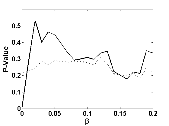
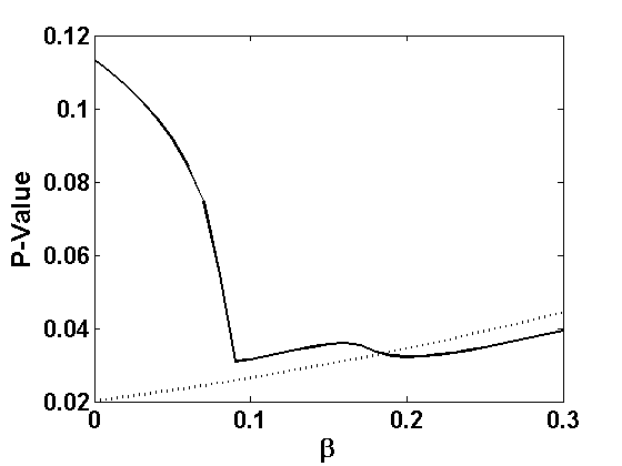
but to check how significant this change is, one might be interested in testing the one-side hypothesis

$$H_{0}:\theta_{2}=\theta_{1}~{}~{}~{}\mbox{against}~{}~{}~{}~{}H_{1}:\theta_{2}>\theta_{1}.$$ (33)

We have applied our proposed Wald-type tests for this problem, as developed in Section 4, to both the full dataset and after deleting the first two outliers from both the groups; the resulting p-values are presented in Figure 4a. Clearly, the classical Wald test results in completely different inference due to the inclusion of these outlying observations – it’s p-value becomes significant from non-significant inference without them (at 95% level). On the other hand, proposed MDPDE based robust Wald-type tests with $\beta>0$ gives stable results (accept the null hypothesis) even in presence of outlying observations.

Table 4: MDPDEs of Poisson parameter $\theta$ for the Adverse Events Data in Table 3
$\beta$
Group 0 0.1 0.3 0.5 0.7 0.9 1
With Treatment 15.00 7.25 6.94 6.35 5.86 6.05 5.70
Outlier Control 18.47 8.25 7.75 7.56 7.53 7.41 7.81
Without Treatment 8.82 7.47 6.44 6.20 6.14 5.58 6.58
Outlier Control 9.65 7.97 7.63 7.61 7.56 7.68 7.75

5.2 Poisson Model for Experimental Trial: Drosophila Data

We next consider another application to the Poisson model with data from an controlled experimental trial with Drosophila flies producing occasional spurious counts. The dataset contains two independent samples on the numbers of recessive lethal mutations observed among the daughters of male flies who are exposed either to a certain degree of chemical to be screened (treatment group) or to control conditions. This dataset has been previously analyzed by many statisticians including Woodruff etΒ al. (1984); Simpson (1989); Basu etΒ al. (2013) who have shown that the response data can be modeled by Poisson distribution, but there are two outlying observations in one sample that affects the likelihood based inference and so the classical Wald test. See Basu etΒ al. (2013, Table 7) for the dataset and the MDPDEs of the Poisson parameters.

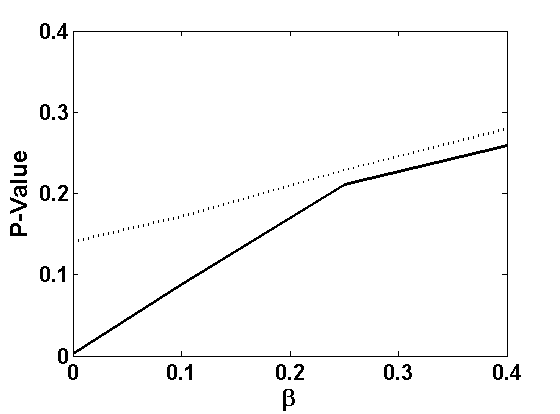
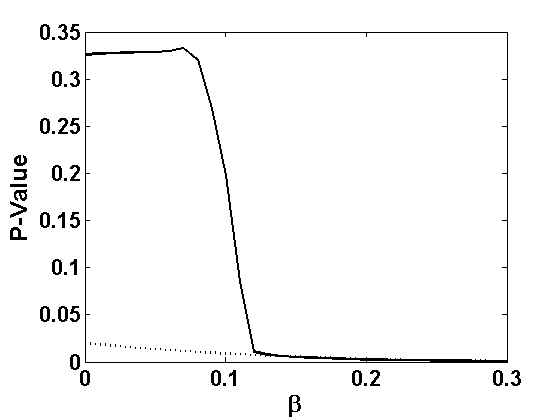
Here, we will apply the proposed Wald-type tests for comparing the Poisson parameters for the two samples, say $\theta_{1}$ and $\theta_{2}$, through testing the one-sided hypothesis in 33. The resulting p-values are presented in Figure 4b. Clearly, in presence of outliers, the classical rejects the null hypothesis indicating that the average number of mutation is significantly more for the second sample, which is the opposite of the true inference obtained after removing these outliers from the second sample. But, the proposed MDPDE based Wald-type tests with $\beta\geq 0.1$ produce robust results even in presence of outliers accepting the null hypothesis.

Refer to caption
(a) Adverse Events Data
Refer to caption
(b) Droshophila Data
Refer to caption
(c) Infant Platelet Count Data
Refer to caption
(d) Hair Zn Content Data
Refer to caption
(e) Cloth Manufacturing data
Refer to caption
(f) Components Life-time Data
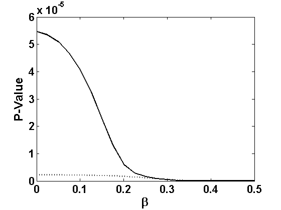
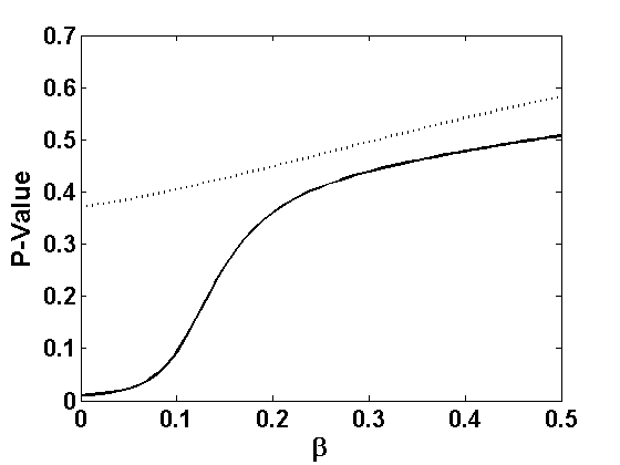
Figure 4: P-values of the proposed Wald-type tests under the real data examples with outliers (solid line) and without outliers (doted line)

5.3 Normal Model for Clinical Trial: Infant Platelet Count Data

We will now present another clinical trial example from Karpatkin etΒ al. (1981) to illustrate the applications under the normal model. This clinical trial was conducted to study if the infant platelet count can be increased by giving steroids to the mothers with autoimmune thrombocytopenia during pregnancy. The study consists of 19 mothers with 12 being given steroid (treatment group) and 7 not given steroid (control group) and the corresponding infant platelet counts (in thousands, per mm3) after delivery are given in Table 5. These can be modeled by a normal model with means $\theta_{1}$, $\theta_{2}$ and the variances $\sigma_{1}^{2}$, $\sigma_{2}^{2}$ for the treatment and control groups respectively. Then, the primary research problem can be solved by testing the one-sided hypothesis in (33) with $\sigma_{1}^{2}$ and $\sigma_{2}^{2}$ being unknown.

Table 5: Infant Platelet count after delivery (in thousands, per mm3) in the Karpatkin etΒ al. (1981) clinical trail study
Treatment 120 124 215 90 67 126 95 190 180 135 399 65
Control 12 20 112 32 60 40 18

The p-values for this testing problem obtained by applying the proposed Wald-type tests, as described in Example 4.1, are presented in Figure 4c for different $\beta\geq 0$. One can easily observe that there is a large outlier value of 399 (thousands) in the treatment group that affects the classical Wald test (at $\beta=0$). However, our MDPDE based proposal with $\beta>0$ produces stable p-value ignoring the effect of the outlying observation.

5.4 Normal Model for Health Study: Hair Zn Content data

Two-sample test under the normal model has many possible applications from which we now present a health study to examine the impact of polluted urban environment over individual health in Sri Lanka. The dataset consist of the zinc (Zn) content of the hair of two independent samples taken from urban (polluted) and rural (unpolluted) Sri Lanka and our target is to check if the Zn content is more for polluted urban residents impacting their health conditions. The dataset was presented in Basu etΒ al. (2015, Table 6) and it has been shown their that each sample can be modeled by normal distributions with means $\theta_{i}$ and variance $\sigma_{i}^{2}$ ($i=1,2$ for rural and urban groups respectively) except for two possible outliers. There is one outlier in each of the samples that affects the MLE based inference while testing for the targeted hypothesis (33) of comparing $\theta_{1}$ and $\theta_{2}$ with unknown $\sigma_{1}^{2}$ and $\sigma_{2}^{2}$.

We have applied the proposed MDPDE based Wald-type test for this problem following Example 4.1 and the resulting p-values are presented in Figure 4d. Clearly, the significance increase of the zinc contents in urban residents cannot be identified by the classical Wald-test in presence of outliers, but our proposal with $\beta\geq 0.1$ gives stable and correct inference ignoring the effect of the outliers.

5.5 Normal Model for Quality Control: Cloth Manufacturing data

Our third and final example with normal model will be in the context of quality control based on the data from the Levi-Strauss clothing manufacturing plant. The dataset consists of 22 measurements on run-up (a percentage measure of wastage in cloth) for each of two particular mills supplying cloths to the plant (Basu etΒ al., 2015, Table 1). To control the quality of the cloths, the plant want to test for the consistency of the run-up measures from the two mills. Since the sample from each mill can be modeled by normal distribution with mean $\theta_{i}$ and variance $\sigma_{i}^{2}$ ($i=1,2$), the objective is then to test for the both sided hypothesis

H0:ΞΈ1=ΞΈ2​againstH1:ΞΈ1β‰ ΞΈ2,:subscript𝐻0subscriptπœƒ1subscriptπœƒ2againstsubscript𝐻1:subscriptπœƒ1subscriptπœƒ2H_{0}:\theta_{1}=\theta_{2}~{}~{}~{}\mbox{against}~{}~{}~{}~{}H_{1}:\theta_{1}\neq\theta_{2}, (34)

with $\sigma_{1}^{2}$ and $\sigma_{2}^{2}$ being unknown under both cases. However, as illustrated in Basu etΒ al. (2015), the dataset contains 3 potential outliers that make the MLE based inference highly non-robust. Hence the classical Wald test rejects the null hypothesis in presence of outliers whereas it accept the null after removing the outliers. When we apply the proposed MDPDE based Wald-type problem, following the description as in Example 3.1, the corresponding p-values (reported in Figure 4e) becomes highly stable for $\beta\geq 1.5$ rejecting the null hypothesis even in presence of the outliers.

5.6 Exponential Model for Reliability Testing: Components Life-time Data

We will end this section with an example of exponential model used in reliability testing between two sets of products’ lifetimes. We will use the (simulated) data from Perng (1978) which consist of the lifetimes (in thousand of hours) of a particular electronic components produced by two different processes (see Table 6). Each sample can be then modeled by exponential distributions with mean $\theta_{i}$ ($i=1,2$). Our objective in reliability testing of the manufacturing process is to test whether the lifetimes for both the process have the same distributions, i.e., if $\theta_{1}=\theta_{2}$ against the both-sided alternatives as in the hypothesis (34). It has been observed that there is no significant difference in the distributions of both the processes and so the null hypothesis should be accepted by any standard test.

Table 6: Lifetimes (in thousand of hours) of a particular electronic components produced by two different processes (Perng, 1978)
Process 1 .044 .134 .142 .158 .216 .625 .649 .658 1.062 1.140 1.159 1.238
Process 2 .060 .174 .237 .272 .335 .391 .670 .902 1.543 1.615 2.013 2.309

Since there is no outliers in this dataset, in order to study the robustness aspect of our proposal we add one outlying value of 20 (assuming a decimal is misplaced by one digit from 2.0) in the second sample. The resulting p-values obtained by the proposed Wald-type tests for both the pure data and with this artificial outlier are presented in Figure 4f for different $\beta$. Clearly, the classical Wald test changes drastically by rejecting null due to insertion of only one outlying observations, but our proposed Wald-type tests with $\beta\geq 0.1$ remains stable and still accept the null hypothesis robustly in presence of the outlier.

6 Simulation Study and the Choice of Tunning Parameter $\beta$

Finally to examine the finite sample performances of our Wald-type tests, we have performed several simulation studies with all the models considered in the previous section for real datasets. However, noting the similarity of the results for different models, for brevity, here we will report the results from only one simulation study under normal model with two-sided alternatives.

We simulate 1000 pair of samples, each of size n=50𝑛50n=50, independently drawn from N​(ΞΈi,1)𝑁subscriptπœƒπ‘–1N(\theta_{i},1) distributions (i=1,2𝑖12i=1,2) and perform the proposed Wald-type tests for testing H0:ΞΈ1=ΞΈ2:subscript𝐻0subscriptπœƒ1subscriptπœƒ2H_{0}:\theta_{1}=\theta_{2} against the two-sided alternative H1:ΞΈ1β‰ ΞΈ2:subscript𝐻1subscriptπœƒ1subscriptπœƒ2H_{1}:\theta_{1}\neq\theta_{2}, once assuming both variances to be known (equal 1) and then assuming variances to be unknown and unequal following Examples 2.1 and 3.1 respectively. 
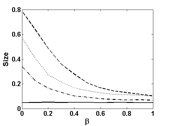
Then, we compute the empirical sizes and powers of the proposed test under these pure data over 100010001000 iterations, where for size calculation we have taken ΞΈ1=ΞΈ2=0subscriptπœƒ1subscriptπœƒ20\theta_{1}=\theta_{2}=0 and for power calculation ΞΈ1=0subscriptπœƒ10\theta_{1}=0, ΞΈ2=1subscriptπœƒ21\theta_{2}=1. Next, to study the robustness performances, we contaminate 100​Ρ%100percentπœ€100\varepsilon\% of second sample in each iteration (for Ξ΅=0.1,0.15,0.2πœ€0.10.150.2\varepsilon=0.1,0.15,0.2) by observations from N​(ΞΈc,1)𝑁subscriptπœƒπ‘1N(\theta_{c},1) distributions and repeat the above simulation to compute empirical sizes and power under contamination. We have taken ΞΈc=3subscriptπœƒπ‘3\theta_{c}=3 and βˆ’33-3 for studying the robustness of size and power respectively. Note that these contamination distributions are not very far from the corresponding true distributions and hence generate reasonably common practical situations. Resulting empirical sizes and powers are reported in Figure 5.

Refer to caption
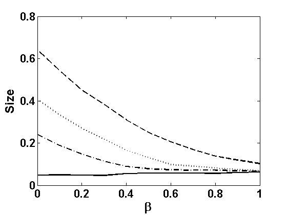
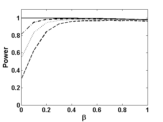
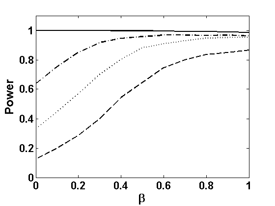
(a) Sizes, known variances
Refer to caption
(b) Sizes, unknown variances
Refer to caption
(c) Powers, known variances
Refer to caption
(d) Powers, unknown variances
Figure 5: Empirical sizes and powers of the proposed Wald-type tests for testing equality of two normal means with both the known and unknown variance case at sample size $n=50$ under pure data (solid line) and with contamination of 10% (dash-doted line), 15% (doted line) and 20% (dashed line)

It can be easily observed from Figure 5 that the size and power of the proposed Wald-type tests under pure data change (increases and decreases respectively) only very slightly with increasing $\beta$, but their stability increases significantly. In particular, under contamination, both size and power of the tests near $\beta=0$, the classical Wald test, changes drastically. But they become stable at larger positive values of $\beta$ for both the cases of known and unknown variances. However, for the cases of known (and correctly specified) variances we get highly stable results near $\beta\approx 0.3,0.4$, whereas we need $\beta\approx 0.5,0.6$ for the case of unknown variances. This is intuitively expected since under the present contamination schemes the variance estimates also changes and so we need more robustness power to get overall stable inference with larger values of $\beta$.

Throughout all our example and simulations above, we have notices that the tuning parameter $\beta$ controls between robustness of the proposed Wald-type tests and its asymptotic contiguous power under pure data. So, we need to chose $\beta$ properly for any practical applications. In particular we note that, in most of the example models, the loss in power is not significant enough at small positive $\beta$, whereas we get highly robust inferences for $\beta\geq 0.3$ (except for few cases with very high contaminations where we may need $\beta\approx 0.4,0.5$). Therefore, an empirical suggestion for the choice of $\beta$ in any application suspecting some contamination could be within the range $\beta\in[0.3,0.5]$ for generating robust inference without significant loss in power.

Although this ad hoc empirical choice of $\beta$ works well enough in most practical datasets suspectable to outliers, many practitioners will prefer a data-driven choice of $\beta$ in case of no idea on the level of contamination in dataset that might produce a better trade-off. In this respect, we note that the performance of the proposed Wald-type tests directly depends on that of the MDPDE (with tuning parameter $\beta$) used in constructing the test statistics. In particular the asymptotic contiguous power of the proposed test has the same nature as the asymptotic efficiency of the corresponding MDPDE whereas all the robustness measures of our tests directly depend on the robustness of the MDPDE through its influence function. So, a suitable data-driven choice of $\beta$ for our Wald-type test statistics also can be equivalently formed by adjusting the trade-off between efficiency and robustness of the MDPDE used. For this second problem, Warwick and Jones (2005) proposed to minimize an estimator of MSE of the MDPDE to chose optimum $\beta$. Based on the first sample $X_{1},\ldots,X_{n}$, they proposed to minimize the estimated MSE

$\displaystyle\widehat{MSE}_{n}(\beta)=\left({{}^{(1)}}\widehat{{\boldsymbol{\theta}}}_{\beta}-{\boldsymbol{\theta}}_{\beta}^{P}\right)^{T}\left({}^{(1)}\widehat{{\boldsymbol{\theta}}}_{\beta}-{\boldsymbol{\theta}}_{\beta}^{P}\right)+\frac{1}{n}Trace\left(\widehat{\boldsymbol{J}}_{\beta,n}^{-1}\widehat{\boldsymbol{K}}_{\beta,n}\widehat{\boldsymbol{J}}_{\beta,n}^{-1}\right)$ (35)

over $\beta$, where ${\boldsymbol{\theta}}_{\beta}^{P}$ is a pilot estimator of the target parameter and $\widehat{\boldsymbol{J}}_{\beta,n}$ and $\widehat{\boldsymbol{K}}_{\beta,n}$ are estimators of the matrices $\boldsymbol{J}_{\beta}$ and $\boldsymbol{K}_{\beta}$ respectively, which can be easily obtained from their expressions by substituting $\boldsymbol{\theta}$ by the MDPDE and integrations by sample means. Although there is no direct choice for ${\boldsymbol{\theta}}_{\beta}^{P}$, Warwick and Jones (2005) suggested, based on an extensive simulation studies, that the MDPDE with $\beta=1$ can serve the purpose well for the i.i.d.Β set-up and we will stick to that suggestion for the present case also (the non-i.i.d.Β cases have been studied in Ghosh and Basu (2013, 2015)). However, the problem in the present two-sample case is that, the optimum $\beta$ obtained by minimizing $\widehat{MSE}_{n}(\beta)$ based on the first sample may not be the same as that obtained for the second sample due to possible different level of contaminations. As a standard solution, we propose the minimization of the total estimated MSE, the sum of the MSE estimates based on two samples separately, over $\beta\in[0,1]$ to obtain the optimum choice of the tuning parameter for the present two-sample testing problem.

Refer to caption
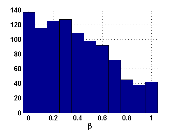
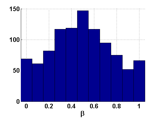
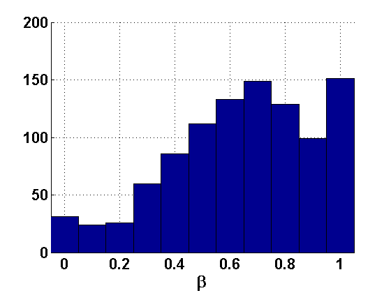
(a) Known var., No contamination
Refer to caption
(b) Known var., 10% contamination
Refer to caption
(c) Known var., 20% contamination
Figure 6: Histograms for optimally chosen tuning parameter $\beta$ under normal models with different contamination levels

We have implemented this proposal for the above simulation study with normal model to check its effectiveness. Figure 6 presents the histograms of the 1000 selected optimum $\beta$ following this proposal for the normal model with known and equal variances under the simulation scheme used for studying size stability above (in Figure 5). Clearly, the mode of these optimum $\beta$s shift from 0 to 1 as the contamination proportion increases yielding the expected trade-off between the power and robustness based on the level of contaminations.

7 Concluding remarks

In this paper, we have considered the problem of testing with two independent samples of i.i.d.Β observations and proposed a class of robust Wald-type tests for both simple and composite hypothesis testing. These Wald-type tests are constructed using the robust minimum density power divergence estimators of the underlying parameters in each sample. The asymptotic and robustness properties of the proposed Wald-type tests have been discussed along with their applications to several important real-life problems like clinical trial, medical experiment, reliability testing and many more.

Although we have discussed all possible types of general two-sample hypotheses, in this paper, we have restricted our attention to the cases where each of the two independent samples is identically distributed. The natural extension of this work will be to develop robust tests for hypotheses involving two independent samples from non-homogeneous populations; this also has many practical applications including comparing the regression lines between two groups of patients in a fixed design clinical trial. Also, one could further explore the possibility of robust hypothesis testing using the minimum density power divergence estimators for two paired samples or for more than two sample cases. we hope to pursue some of this possible extensions in our future research.

Appendix A Proof of Results

A.1 Proof of Theorem 2.1

Using the asymptotic distribution of $\sqrt{n}(^{(1)}\widehat{{\boldsymbol{\theta}}}_{\beta}-{\boldsymbol{\theta}}_{1})$ and $\sqrt{n}(^{(2)}\widehat{{\boldsymbol{\theta}}}_{\beta}-{\boldsymbol{\theta}}_{2})$, we have

$$\sqrt{\frac{mn}{m+n}}\left({}^{(1)}\widehat{{\boldsymbol{\theta}}}_{\beta}-{\boldsymbol{\theta}}_{1}\right)\displaystyle\underset{m,n\rightarrow\infty}{\overset{\mathcal{L}}{\longrightarrow}}N(\boldsymbol{0}_{p},\omega{\boldsymbol{\Sigma}}_{\beta}({\boldsymbol{\theta}}_{1}))$$

and

$$\sqrt{\frac{mn}{m+n}}\left({}^{(2)}\widehat{{\boldsymbol{\theta}}}_{\beta}-{\boldsymbol{\theta}}_{2}\right)\displaystyle\underset{m,n\rightarrow\infty}{\overset{\mathcal{L}}{\longrightarrow}}N(\boldsymbol{0}_{p},(1-\omega){\boldsymbol{\Sigma}}_{\beta}({\boldsymbol{\theta}}_{2})).$$

Hence under $H_{0}:{\boldsymbol{\theta}}_{1}={\boldsymbol{\theta}}_{2}={\boldsymbol{\theta}}_{0}$, we get

$$\sqrt{\frac{mn}{m+n}}\left({}^{(1)}\widehat{{\boldsymbol{\theta}}}_{\beta}-^{(1)}\widehat{{\boldsymbol{\theta}}}_{\beta}\right)\underset{m,n\rightarrow\infty}{\overset{\mathcal{L}}{\longrightarrow}}N(\boldsymbol{0}_{p},{\boldsymbol{\Sigma}}_{\beta}({\boldsymbol{\theta}}_{0})).$$

Further, under $H_{0}$, ${}^{(0)}\widehat{{\boldsymbol{\theta}}}_{\beta}~{}\displaystyle{\overset{\mathcal{P}}{\rightarrow}}~{}{\boldsymbol{\theta}}_{0}$ as $m+n\rightarrow\infty$. Then the theorem follows using the continuity of the matrix ${\boldsymbol{\Sigma}}_{\beta}({\boldsymbol{\theta}})$. $\square$

A.2 Proof of Theorem 2.2

Note that, ${}^{(0)}\widehat{{\boldsymbol{\theta}}}_{\beta}\underset{n,m\rightarrow\infty}{\overset{\mathcal{P}}{\longrightarrow}}{\boldsymbol{\theta}}_{3}$ and hence the asymptotic distribution of $l_{{}^{(0)}\widehat{{\boldsymbol{\theta}}}_{\beta},\beta}^{\ast}(^{(1)}\widehat{{\boldsymbol{\theta}}}_{\beta},^{(2)}\widehat{{\boldsymbol{\theta}}}_{\beta})$ is the same as that of $l_{{\boldsymbol{\theta}}_{3},\beta}^{\ast}(^{(1)}\widehat{{\boldsymbol{\theta}}}_{\beta},^{(2)}\widehat{{\boldsymbol{\theta}}}_{\beta})$. Now, a suitable Taylor series expansion leads to

$\displaystyle l_{{\boldsymbol{\theta}}_{3},\beta}^{\ast}(^{(1)}\widehat{{\boldsymbol{\theta}}}_{\beta},^{(2)}\widehat{{\boldsymbol{\theta}}}_{\beta})-l_{{\boldsymbol{\theta}}_{3},\beta}^{\ast}({\boldsymbol{\theta}}_{1},{\boldsymbol{\theta}}_{2})$ $\displaystyle=$ $\displaystyle\left({}^{(1)}\widehat{{\boldsymbol{\theta}}}_{\beta}-{\boldsymbol{\theta}}_{1}\right)^{T}\frac{\partial}{\partial{\boldsymbol{\theta}}_{1}}l_{{\boldsymbol{\theta}}_{3},\beta}^{\ast}({\boldsymbol{\theta}}_{1},{\boldsymbol{\theta}}_{2})+\left({}^{(2)}\widehat{{\boldsymbol{\theta}}}_{\beta}-{\boldsymbol{\theta}}_{2}\right)^{T}\frac{\partial}{\partial{\boldsymbol{\theta}}_{2}}l_{{\boldsymbol{\theta}}_{3},\beta}^{\ast}({\boldsymbol{\theta}}_{1},{\boldsymbol{\theta}}_{2})$
$\displaystyle+o_{P}\left(||^{(1)}\widehat{{\boldsymbol{\theta}}}_{\beta}-{\boldsymbol{\theta}}_{1}||^{2}\right)+o_{P}\left(||^{(2)}\widehat{{\boldsymbol{\theta}}}_{\beta}-{\boldsymbol{\theta}}_{2}||^{2}\right)$
$\displaystyle=$ $\displaystyle 2\left({}^{(1)}\widehat{{\boldsymbol{\theta}}}_{\beta}-{\boldsymbol{\theta}}_{1}\right)^{T}{\boldsymbol{\Sigma}}_{\beta}({\boldsymbol{\theta}}_{3})^{-1}({\boldsymbol{\theta}}_{1}-{\boldsymbol{\theta}}_{2})-2\left({}^{(2)}\widehat{{\boldsymbol{\theta}}}_{\beta}-{\boldsymbol{\theta}}_{2}\right)^{T}{\boldsymbol{\Sigma}}_{\beta}({\boldsymbol{\theta}}_{3})^{-1}({\boldsymbol{\theta}}_{1}-{\boldsymbol{\theta}}_{2})$
$\displaystyle+o_{P}\left(||^{(1)}\widehat{{\boldsymbol{\theta}}}_{\beta}-{\boldsymbol{\theta}}_{1}||^{2}\right)+o_{P}\left(||^{(2)}\widehat{{\boldsymbol{\theta}}}_{\beta}-{\boldsymbol{\theta}}_{2}||^{2}\right)$
$\displaystyle=$ $\displaystyle 2\left[\left({}^{(1)}\widehat{{\boldsymbol{\theta}}}_{\beta}-^{(2)}\widehat{{\boldsymbol{\theta}}}_{\beta}\right)-\left({\boldsymbol{\theta}}_{1}-{\boldsymbol{\theta}}_{2}\right)\right]^{T}{\boldsymbol{\Sigma}}_{\beta}({\boldsymbol{\theta}}_{3})^{-1}({\boldsymbol{\theta}}_{1}-{\boldsymbol{\theta}}_{2})$
$\displaystyle+o_{P}\left(||^{(1)}\widehat{{\boldsymbol{\theta}}}_{\beta}-{\boldsymbol{\theta}}_{1}||^{2}\right)+o_{P}\left(||^{(2)}\widehat{{\boldsymbol{\theta}}}_{\beta}-{\boldsymbol{\theta}}_{2}||^{2}\right).$

Then, the theorem follows from the above expression by noting that

$$\sqrt{\frac{mn}{m+n}}\left[\left({}^{(1)}\widehat{{\boldsymbol{\theta}}}_{\beta}-^{(2)}\widehat{{\boldsymbol{\theta}}}_{\beta}\right)-\left({\boldsymbol{\theta}}_{1}-{\boldsymbol{\theta}}_{2}\right)\right]\underset{n,m\rightarrow\infty}{\overset{\mathcal{L}}{\longrightarrow}}\mathcal{N}\left(0,\left[\omega{\boldsymbol{\Sigma}}_{\beta}({\boldsymbol{\theta}}_{1})+(1-\omega){\boldsymbol{\Sigma}}_{\beta}({\boldsymbol{\theta}}_{2})\right]\right),$$

as $m,n\rightarrow\infty$ at any 𝜽1β‰ πœ½2subscript𝜽1subscript𝜽2{\boldsymbol{\theta}}_{1}\neq{\boldsymbol{\theta}}_{2}. Here, the last convergence follows from the asymptotic distributions of the MDPDEs ${}^{(1)}\widehat{{\boldsymbol{\theta}}}_{\beta}$ and ${}^{(2)}\widehat{{\boldsymbol{\theta}}}_{\beta}$. $\square$

A.3 Proof of Theorem 2.5

Using the asymptotic distribution of $\sqrt{n}(^{(1)}\widehat{{\boldsymbol{\theta}}}_{\beta}-{\boldsymbol{\theta}}_{1,n})$ and $\sqrt{n}(^{(2)}\widehat{{\boldsymbol{\theta}}}_{\beta}-{\boldsymbol{\theta}}_{2,m})$ under $H_{1,n,m}$ and continuity of ${\boldsymbol{\Sigma}}_{\beta}({\boldsymbol{\theta}}_{0})$, we have ${}^{(2)}\widehat{{\boldsymbol{\theta}}}_{\beta}\underset{m\rightarrow\infty}{\overset{\mathcal{P}}{\longrightarrow}}{\boldsymbol{\theta}}_{0}$,

$$\sqrt{\frac{mn}{m+n}}\left({}^{(1)}\widehat{{\boldsymbol{\theta}}}_{\beta}-{\boldsymbol{\theta}}_{0}\right)\underset{m,n\rightarrow\infty}{\overset{\mathcal{L}}{\longrightarrow}}N(\sqrt{\omega}{\boldsymbol{\Delta}}_{1},\omega{\boldsymbol{\Sigma}}_{\beta}({\boldsymbol{\theta}}_{0}))$$

and

$$\sqrt{\frac{mn}{m+n}}\left({}^{(2)}\widehat{{\boldsymbol{\theta}}}_{\beta}-{\boldsymbol{\theta}}_{0}\right)\underset{m,n\rightarrow\infty}{\overset{\mathcal{L}}{\longrightarrow}}N(\sqrt{1-\omega}{\boldsymbol{\Delta}}_{2},(1-\omega){\boldsymbol{\Sigma}}_{\beta}({\boldsymbol{\theta}}_{0})).$$

Hence, under $H_{1,n,m}$, we get

$$\sqrt{\frac{mn}{m+n}}\left({}^{(1)}\widehat{{\boldsymbol{\theta}}}_{\beta}-^{(1)}\widehat{{\boldsymbol{\theta}}}_{\beta}\right)\underset{m,n\rightarrow\infty}{\overset{\mathcal{L}}{\longrightarrow}}N(\sqrt{\omega}{\boldsymbol{\Delta}}_{1}-\sqrt{1-\omega}{\boldsymbol{\Delta}}_{2},{\boldsymbol{\Sigma}}_{\beta}({\boldsymbol{\theta}}_{0})),$$

from which the theorem follows immediately. $\square$

A.4 Proof of Theorem 2.6

We will only prove the case $(D_{1},D_{2})=(F_{1,m,\varepsilon,x}^{P},F_{2,n,\varepsilon,y}^{P})$. Other two cases will follow similarly.

Let us denote ${\boldsymbol{\theta}}_{1,n}^{\ast}=\boldsymbol{U}_{\beta}(F_{1,m,\varepsilon,x}^{P})$ and ${\boldsymbol{\theta}}_{2,m}^{\ast}=\boldsymbol{U}_{\beta}(F_{2,n,\varepsilon,y}^{P})$. Then using the continuity of ${\boldsymbol{\Sigma}}_{\beta}({\boldsymbol{\theta}}_{0})$, we get under $(D_{1},D_{2})=(F_{1,m,\varepsilon,x}^{P},F_{2,n,\varepsilon,y}^{P})$, the asymptotic distribution of $\sqrt{n}(^{(1)}\widehat{{\boldsymbol{\theta}}}_{\beta}-{\boldsymbol{\theta}}_{1,n}^{\ast})$ and $\sqrt{n}(^{(2)}\widehat{{\boldsymbol{\theta}}}_{\beta}-{\boldsymbol{\theta}}_{2,m}^{\ast})$ are both $p$-variate normal with mean zero and variance ${\boldsymbol{\Sigma}}_{\beta}({\boldsymbol{\theta}}_{0})$. Further, suitable Taylor series expansion yields

$\displaystyle{\boldsymbol{\theta}}_{1,n}^{\ast}$ $\displaystyle=$ $\displaystyle{\boldsymbol{\theta}}_{1,n}+\frac{\varepsilon}{\sqrt{n}}\mathcal{IF}(x;\boldsymbol{U}_{\beta},F_{{\boldsymbol{\theta}}_{1,n}})+o(n^{-1/2})$
$\displaystyle=$ $\displaystyle{\boldsymbol{\theta}}_{0}+\frac{{\boldsymbol{\Delta}}_{1}}{\sqrt{n}}+\frac{\varepsilon}{\sqrt{n}}\mathcal{IF}(x;\boldsymbol{U}_{\beta},F_{{\boldsymbol{\theta}}_{1,n}})+o(n^{-1/2})$
$\displaystyle=$ $\displaystyle{\boldsymbol{\theta}}_{0}+\frac{\widetilde{{\boldsymbol{\Delta}}_{1}}}{\sqrt{n}}+o(n^{-1/2}).$

Similarly, we have

$${\boldsymbol{\theta}}_{2,m}^{\ast}={\boldsymbol{\theta}}_{0}+\frac{\widetilde{{\boldsymbol{\Delta}}_{2}}}{\sqrt{n}}+o(n^{-1/2}).$$

Combining all these, we get

$$\sqrt{\frac{mn}{m+n}}\left({}^{(1)}\widehat{{\boldsymbol{\theta}}}_{\beta}-{\boldsymbol{\theta}}_{0}\right)\displaystyle\underset{m,n\rightarrow\infty}{\overset{\mathcal{L}}{\longrightarrow}}N(\sqrt{\omega}\widetilde{{\boldsymbol{\Delta}}}_{1},\omega{\boldsymbol{\Sigma}}_{\beta}({\boldsymbol{\theta}}_{0}))$$

and

$$\sqrt{\frac{mn}{m+n}}\left({}^{(2)}\widehat{{\boldsymbol{\theta}}}_{\beta}-{\boldsymbol{\theta}}_{0}\right)\displaystyle\underset{m,n\rightarrow\infty}{\overset{\mathcal{L}}{\longrightarrow}}N(\sqrt{1-\omega}\widetilde{{\boldsymbol{\Delta}}}_{2},(1-\omega){\boldsymbol{\Sigma}}_{\beta}({\boldsymbol{\theta}}_{0})).$$

Hence, under $(D_{1},D_{2})=(F_{1,m,\varepsilon,x}^{P},F_{2,n,\varepsilon,y}^{P})$, we get

$$\sqrt{\frac{mn}{m+n}}\left({}^{(1)}\widehat{{\boldsymbol{\theta}}}_{\beta}-^{(1)}\widehat{{\boldsymbol{\theta}}}_{\beta}\right)\underset{m,n\rightarrow\infty}{\overset{\mathcal{L}}{\longrightarrow}}N(\sqrt{\omega}\widetilde{{\boldsymbol{\Delta}}}_{1}-\sqrt{1-\omega}\widetilde{{\boldsymbol{\Delta}}}_{2},{\boldsymbol{\Sigma}}_{\beta}({\boldsymbol{\theta}}_{0}))$$

and hence the theorem follows immediately. $\square$

A.5 Proof of Theorem 3.1

Using suitable Taylor series expansion, we get

$\displaystyle\boldsymbol{\psi}(^{(1)}\widehat{{\boldsymbol{\theta}}}_{\beta},^{(2)}\widehat{{\boldsymbol{\theta}}}_{\beta})$ $\displaystyle=$ $\displaystyle\boldsymbol{\psi}({\boldsymbol{\theta}}_{1},{\boldsymbol{\theta}}_{2})+\boldsymbol{\Psi}_{1}({\boldsymbol{\theta}}_{1},{\boldsymbol{\theta}}_{2})^{T}(^{(1)}\widehat{{\boldsymbol{\theta}}}_{\beta}-{\boldsymbol{\theta}}_{1})+\boldsymbol{\Psi}_{2}({\boldsymbol{\theta}}_{1},{\boldsymbol{\theta}}_{2})^{T}(^{(2)}\widehat{{\boldsymbol{\theta}}}_{\beta}-{\boldsymbol{\theta}}_{2})$ (36)
$\displaystyle~{}~{}~{}~{}~{}~{}~{}~{}+o_{P}\left(||^{(1)}\widehat{{\boldsymbol{\theta}}}_{\beta}-{\boldsymbol{\theta}}_{1}||\right)+o_{P}\left(||^{(2)}\widehat{{\boldsymbol{\theta}}}_{\beta}-{\boldsymbol{\theta}}_{2}||\right).$

Now, from the asymptotic distribution of $\sqrt{n}(^{(1)}\widehat{{\boldsymbol{\theta}}}_{\beta}-{\boldsymbol{\theta}}_{1})$ and $\sqrt{n}(^{(2)}\widehat{{\boldsymbol{\theta}}}_{\beta}-{\boldsymbol{\theta}}_{2})$ it follows that

$$\sqrt{\frac{mn}{m+n}}\boldsymbol{\Psi}_{1}({\boldsymbol{\theta}}_{1},{\boldsymbol{\theta}}_{2})^{T}\left({}^{(1)}\widehat{{\boldsymbol{\theta}}}_{\beta}-{\boldsymbol{\theta}}_{1}\right)\displaystyle\underset{m,n\rightarrow\infty}{\overset{\mathcal{L}}{\longrightarrow}}N(0,\omega\boldsymbol{\Psi}_{1}({\boldsymbol{\theta}}_{1},{\boldsymbol{\theta}}_{2})^{T}{\boldsymbol{\Sigma}}_{\beta}({\boldsymbol{\theta}}_{1})\boldsymbol{\Psi}_{1}({\boldsymbol{\theta}}_{1},{\boldsymbol{\theta}}_{2}))$$

and

$$\sqrt{\frac{mn}{m+n}}\boldsymbol{\Psi}_{2}({\boldsymbol{\theta}}_{1},{\boldsymbol{\theta}}_{2})^{T}\left({}^{(2)}\widehat{{\boldsymbol{\theta}}}_{\beta}-{\boldsymbol{\theta}}_{2}\right)\displaystyle\underset{m,n\rightarrow\infty}{\overset{\mathcal{L}}{\longrightarrow}}N(0,(1-\omega)\boldsymbol{\Psi}_{2}({\boldsymbol{\theta}}_{1},{\boldsymbol{\theta}}_{2})^{T}{\boldsymbol{\Sigma}}_{\beta}({\boldsymbol{\theta}}_{2})\boldsymbol{\Psi}_{2}({\boldsymbol{\theta}}_{1},{\boldsymbol{\theta}}_{2})).$$

Hence under $H_{0}:\boldsymbol{\psi}({\boldsymbol{\theta}}_{1},{\boldsymbol{\theta}}_{2})=\boldsymbol{0}_{r}$, we get

$$\sqrt{\frac{mn}{m+n}}\boldsymbol{\psi}\left({}^{(1)}\widehat{{\boldsymbol{\theta}}}_{\beta},^{(2)}\widehat{{\boldsymbol{\theta}}}_{\beta}\right)\underset{m,n\rightarrow\infty}{\overset{\mathcal{L}}{\longrightarrow}}N(\boldsymbol{0}_{r},\widetilde{{\boldsymbol{\Sigma}}_{\beta}}({\boldsymbol{\theta}}_{1},{\boldsymbol{\theta}}_{2})).$$

Finally, by the consistency of the MDPDEs and the continuity of the matrices $\boldsymbol{\Psi}_{1}$, $\boldsymbol{\Psi}_{2}$ and ${\boldsymbol{\Sigma}}_{\beta}$, it follows that $\widetilde{{\boldsymbol{\Sigma}}_{\beta}}(^{(1)}\widehat{{\boldsymbol{\theta}}}_{\beta}^{(2)}\widehat{{\boldsymbol{\theta}}}_{\beta})~{}\displaystyle{\overset{\mathcal{P}}{\rightarrow}}~{}\widetilde{{\boldsymbol{\Sigma}}_{\beta}}({\boldsymbol{\theta}}_{1},{\boldsymbol{\theta}}_{2})$ as $m+n\rightarrow\infty$, from which the theorem follows immediately. $\square$

A.6 Proof of Theorem 3.2

Using an appropriate Taylor series expansion, we get

$\displaystyle\widetilde{l^{*}}(^{(1)}\widehat{{\boldsymbol{\theta}}}_{\beta},^{(2)}\widehat{{\boldsymbol{\theta}}}_{\beta})-\widetilde{l^{*}}({\boldsymbol{\theta}}_{1},{\boldsymbol{\theta}}_{2}=\left({}^{(1)}\widehat{{\boldsymbol{\theta}}}_{\beta}-{\boldsymbol{\theta}}_{1}\right)^{T}\frac{\partial}{\partial{\boldsymbol{\theta}}_{1}}\widetilde{l^{*}}({\boldsymbol{\theta}}_{1},{\boldsymbol{\theta}}_{2})+\left({}^{(2)}\widehat{{\boldsymbol{\theta}}}_{\beta}-{\boldsymbol{\theta}}_{2}\right)^{T}\frac{\partial}{\partial{\boldsymbol{\theta}}_{2}}\widetilde{l^{*}}({\boldsymbol{\theta}}_{1},{\boldsymbol{\theta}}_{2})$
$\displaystyle~{}~{}~{}~{}~{}~{}~{}~{}~{}~{}~{}~{}~{}~{}~{}~{}~{}~{}~{}~{}~{}~{}~{}~{}~{}~{}~{}~{}+o_{P}\left(||^{(1)}\widehat{{\boldsymbol{\theta}}}_{\beta}-{\boldsymbol{\theta}}_{1}||^{2}\right)+o_{P}\left(||^{(2)}\widehat{{\boldsymbol{\theta}}}_{\beta}-{\boldsymbol{\theta}}_{2}||^{2}\right)$
$\displaystyle=$ $\displaystyle 2\left({}^{(1)}\widehat{{\boldsymbol{\theta}}}_{\beta}-{\boldsymbol{\theta}}_{1}\right)^{T}\boldsymbol{\Psi}_{1}({\boldsymbol{\theta}}_{1},{\boldsymbol{\theta}}_{2})\widetilde{{\boldsymbol{\Sigma}}_{\beta}}({\boldsymbol{\theta}}_{1},{\boldsymbol{\theta}}_{2})^{-1}\boldsymbol{\psi}({\boldsymbol{\theta}}_{1},{\boldsymbol{\theta}}_{2})+2\left({}^{(2)}\widehat{{\boldsymbol{\theta}}}_{\beta}-{\boldsymbol{\theta}}_{2}\right)^{T}\boldsymbol{\Psi}_{2}({\boldsymbol{\theta}}_{1},{\boldsymbol{\theta}}_{2})\widetilde{{\boldsymbol{\Sigma}}_{\beta}}({\boldsymbol{\theta}}_{1},{\boldsymbol{\theta}}_{2})^{-1}\boldsymbol{\psi}({\boldsymbol{\theta}}_{1},{\boldsymbol{\theta}}_{2})$
$\displaystyle~{}~{}~{}~{}~{}~{}~{}~{}~{}~{}~{}~{}~{}~{}~{}~{}~{}~{}~{}~{}~{}~{}~{}~{}~{}~{}+o_{P}\left(||^{(1)}\widehat{{\boldsymbol{\theta}}}_{\beta}-{\boldsymbol{\theta}}_{1}||^{2}\right)+o_{P}\left(||^{(2)}\widehat{{\boldsymbol{\theta}}}_{\beta}-{\boldsymbol{\theta}}_{2}||^{2}\right)$
$\displaystyle=$ $\displaystyle 2\left[\boldsymbol{\Psi}_{1}({\boldsymbol{\theta}}_{1},{\boldsymbol{\theta}}_{2})^{T}\left({}^{(1)}\widehat{{\boldsymbol{\theta}}}_{\beta}-{\boldsymbol{\theta}}_{1}\right)+\boldsymbol{\Psi}_{2}({\boldsymbol{\theta}}_{1},{\boldsymbol{\theta}}_{2})^{T}\left({}^{(2)}\widehat{{\boldsymbol{\theta}}}_{\beta}-{\boldsymbol{\theta}}_{2}\right)\right]^{T}\widetilde{{\boldsymbol{\Sigma}}_{\beta}}({\boldsymbol{\theta}}_{1},{\boldsymbol{\theta}}_{2})^{-1}\boldsymbol{\psi}({\boldsymbol{\theta}}_{1},{\boldsymbol{\theta}}_{2})$
$\displaystyle~{}~{}~{}~{}~{}~{}~{}~{}~{}~{}~{}~{}~{}~{}~{}~{}~{}~{}~{}~{}~{}~{}~{}~{}~{}~{}~{}~{}+o_{P}\left(||^{(1)}\widehat{{\boldsymbol{\theta}}}_{\beta}-{\boldsymbol{\theta}}_{1}||^{2}\right)+o_{P}\left(||^{(2)}\widehat{{\boldsymbol{\theta}}}_{\beta}-{\boldsymbol{\theta}}_{2}||^{2}\right).$

Then, the theorem follows from the asymptotic distributions of the MDPDEs ${}^{(1)}\widehat{{\boldsymbol{\theta}}}_{\beta}$ and ${}^{(2)}\widehat{{\boldsymbol{\theta}}}_{\beta}$. $\square$

A.7 Proof of Theorem 3.4

Using the asymptotic distribution of $\sqrt{n}(^{(1)}\widehat{{\boldsymbol{\theta}}}_{\beta}-{\boldsymbol{\theta}}_{1,n})$ and $\sqrt{n}(^{(2)}\widehat{{\boldsymbol{\theta}}}_{\beta}-{\boldsymbol{\theta}}_{2,m})$ under $H_{1,n,m}$ and continuity of ${\boldsymbol{\Sigma}}_{\beta}({\boldsymbol{\theta}}_{0})$, we have, as $m,n\rightarrow\infty$, ${}^{(2)}\widehat{{\boldsymbol{\theta}}}_{\beta}\displaystyle\mathop{\rightarrow}^{\mathcal{P}}{\boldsymbol{\theta}}_{0}$,

$$\sqrt{\frac{mn}{m+n}}\left({}^{(1)}\widehat{{\boldsymbol{\theta}}}_{\beta}-{\boldsymbol{\theta}}_{10}\right)\displaystyle\underset{m,n\rightarrow\infty}{\overset{\mathcal{L}}{\longrightarrow}}N(\sqrt{\omega}{\boldsymbol{\Delta}}_{1},\omega{\boldsymbol{\Sigma}}_{\beta}({\boldsymbol{\theta}}_{1}))$$

and

$$\sqrt{\frac{mn}{m+n}}\left({}^{(2)}\widehat{{\boldsymbol{\theta}}}_{\beta}-{\boldsymbol{\theta}}_{20}\right)\displaystyle\underset{m,n\rightarrow\infty}{\overset{\mathcal{L}}{\longrightarrow}}N(\sqrt{1-\omega}{\boldsymbol{\Delta}}_{2},(1-\omega){\boldsymbol{\Sigma}}_{\beta}({\boldsymbol{\theta}}_{2})).$$

Hence, following the proof of Theorem 2.5, we get under $H_{1,n,m}$

$$\sqrt{\frac{mn}{m+n}}\boldsymbol{\psi}\left({}^{(1)}\widehat{{\boldsymbol{\theta}}}_{\beta},^{(2)}\widehat{{\boldsymbol{\theta}}}_{\beta}\right)\underset{m,n\rightarrow\infty}{\overset{\mathcal{L}}{\longrightarrow}}N\left(\left[\sqrt{\omega}\boldsymbol{\Psi}_{1}({\boldsymbol{\theta}}_{1},{\boldsymbol{\theta}}_{2})^{T}{\boldsymbol{\Delta}}_{1}+\sqrt{1-\omega}\boldsymbol{\Psi}_{2}({\boldsymbol{\theta}}_{1},{\boldsymbol{\theta}}_{2})^{T}{\boldsymbol{\Delta}}_{2}\right],\widetilde{{\boldsymbol{\Sigma}}_{\beta}}({\boldsymbol{\theta}}_{1},{\boldsymbol{\theta}}_{2})\right),$$

from which the theorem follows immediately. $\square$

A.8 Proof of Theorems 3.6 and 3.7

These proofs are similar to that of Theorems 2.6 and 2.7 and hence omitted. $\square$

References

  • Basu etΒ al. (1998) Basu, A., Harris, I. R., Hjort, N. L., and Jones, M. C. (1998). Robust and efficient estimation by minimising a density power divergence. Biometrika, 85, 549–559.
  • Basu etΒ al. (2013) Basu, A., Mandal, A., Martin, N. and Pardo, L. (2013). Testing statistical hypotheses based on the density power divergence. Annals of Institute of Statistical Mathematics, 65, 319–348.
  • Basu etΒ al. (2015) Basu, A., Mandal, A., Martin, N. and Pardo, L. (2015). Robust tests for the equality of two normal means based on the density power divergence. Metrika, 78(5), 611–634.
  • Basu etΒ al. (2016) Basu, A., Mandal, A., Martin, N. and Pardo, L. (2016) Generalized Wald-type tests based on minimum density power divergence estimators. Statistics, 50(1), 1–26.
  • Basu etΒ al. (2011) Basu, A., Shioya, H. and Park, C. (2011). Statistical Inference: The Minimum Distance Approach. Chapman & Hall/CRC, Boca Raton, FL.
  • Ghosh and Basu (2013) Ghosh, A., and Basu, A. (2013). Robust estimation for independent non-homogeneous observations using density power divergence with applications to linear regression. Electronic Journal of Statistics, 7, 2420–2456.
  • Ghosh and Basu (2015) Ghosh, A., and Basu, A. (2015). Robust estimation for non-homogeneous data and the selection of the optimal tuning parameter: the density power divergence approach. Journal of Applied Statistics, 42(9), 2056–2072.
  • Ghosh et al. (2015) Ghosh, A., Basu, A., and Pardo, L. (2015). On the robustness of a divergence based test of simple statistical hypotheses. Journal of Statistical Planning and Inference, 116, 91–108.
  • Ghosh et al. (2016) Ghosh, A., Mandal, A., Martin, N. and Pardo, L. (2016). Influence analysis of robust Wald-type tests. Journal of Multivariate Analysis, 147, 102–126.
  • Hampel etΒ al. (1986) Hampel, F.Β R., Ronchetti, E., Rousseeuw, P.Β J., and Stahel W.(1986). Robust Statistics: The Approach Based on Influence Functions. New York, USA: John Wiley & Sons.
  • Heritier and Ronchetti (1994) Heritier, S. and Ronchetti, E. (1994). Robust bounded-influence tests in general parametric models. Journal of the American Statistical AssociationΒ 89, 897–904.
  • Huber-Carol (1970) Huber-Carol, C. (1970). Etude asymptotique de tests robustes. Ph.Β D. thesis, ETH, Zurich.
  • Karpatkin etΒ al. (1981) Karpatkin, M., Porges, R. F., and Karpatkin, S. (1981). Platelet counts in infants of women with autoimmune thrombocytopenia: effect of steroid administration to the mother. New England Journal of Medicine, 305(16), 936-939.
  • Kerstjens etΒ al. (2012) Kerstjens , H.A.M., Engel , M., Dahl , R., Paggiaro, P., Beck, E., Vandewalker, M., Sigmund, R., Seibold, W., Moroni-Zentgraf, P., and Bateman, E.D. (2012). Tiotropium in Asthma Poorly Controlled with Standard Combination Therapy New England Journal of Medicine, 367, 1198–1207.
  • Kotz etΒ al. (1967) Kotz, S., Johnson, N.Β L., and Boyd, D.Β W. (1967). Series representations of distributions of quadratic forms in normal variables.Β I.Β Non-central case. Annals of Mathematical StatisticsΒ 38, 838–848.
  • Lehmann (1983) Lehmann, E.Β L. (1983). Theory of Point Estimation. John Wiley & Sons.
  • Pardo (2006) Pardo, L. (2006). Statistical Inference based on Divergences. CRC/Chapman-Hall.
  • Perng (1978) Perng, S. K. (1978). A test for equality of two exponential distributions. Statistica neerlandica, 32(2), 93-102.
  • Simpson (1989) Simpson, D.Β G. (1989). Hellinger deviance test: efficiency, breakdown points, and examples. Journal of the American Statistical AssociationΒ  84, 107–113.
  • Toma and Broniatowski (2011) Toma, A., and Broniatowski, M. (2011). Dual divergence estimators and tests: robustness results. Journal of Multivariate Analysis, 102(1), 20–36
  • Warwick and Jones (2005) Warwick, J., and Jones, M.Β C. (2005). Choosing a robustness tuning parameter. Journal of Statistical Computation and Simulation, 75, 581–588.
  • Woodruff etΒ al. (1984) Woodruff, R.Β C., Mason, J.Β M., Valencia, R., and Zimmering, A. (1984). Chemical mutagenesis testing in drosophila β€” I: Comparison of positive and negative control data for sex-linked recessive lethal mutations and reciprocal translocations in three laboratories. Environmental MutagenesisΒ 6, 189–202.