Time-invariant LDPC convolutional codes

Abstract

Spatially coupled codes have been shown to universally achieve the capacity for a large class of channels. Many variants of such codes have been introduced to date. We discuss a further such variant that is particularly simple and is determined by a very small number of parameters. More precisely, we consider time-invariant low-density convolutional codes with very large constraint lengths.

We show via simulations that, despite their extreme simplicity, such codes still show the threshold saturation behavior known from the spatially coupled codes discussed in the literature. Further, we show how the size of the typical minimum stopping set is related to basic parameters of the code. Due to their simplicity and good performance, these codes might be attractive from an implementation perspective.

I Introduction

Spatially coupled codes have been shown to universally achieve the capacity for a large class of channels, [1, 2, 3, 4]. Many variants of such codes have been introduced to date. For the purpose of analysis it is convenient to consider highly random ensembles. For implementation purposes it is convenient to eliminate as much randomness as possible, e.g., by considering constructions based on protographs.

We ask how much “randomness” is required for such codes to perform well. A natural setting is to look at the origins of spatially coupled codes and to consider low-density parity-check (LDPC) convolutional codes with large constraint lengths. But rather than considering time-variant LDPC convolutional codes, we consider time-invariant such codes (and hence the number of parameters that describe such codes is very small). As we will see, even these extremely simple codes exhibit in simulations the threshold saturation phenomenon that is well-known from the standard spatially coupled codes discussed in the literature.

Let us recall. LDPC block codes are linear codes defined by parity-check matrices where the number of non-zero elements per parity-check is small and independent of the blocklength. Due to the small degrees of the checks such codes can be decoded “well” by a message-passing decoder. To be more precise: For well-designed ensembles, the threshold (when we consider ensembles of codes whose blocklength tends to infinity) under belief propagation decoding is close to the Shannon limit, [5, 6]. Nevertheless this threshold is typically strictly smaller than the threshold that would be achievable if we were able to implement maximum a posteriori (MAP) decoding, which is the optimal decoding strategy.

LDPC convolutional codes can be seen as convolutional codes (with very large constraint lengths) defined by parity-check equations with only a small number of non-zero taps (and the number of taps is independent of the constraint length). Standard convolutional codes are typically decoded by means of the Viterbi algorithm, whose complexity is exponential in the constraint length. For the codes that we consider the constraint length is hundreds or even thousands. Decoding via the Viterbi algorithm is therefore not feasible. But, just as for LDPC block codes, these codes can be decoded “well” via a message-passing algorithm due to the low-density nature of the parity-checks. There is one big difference to block codes, however. Whereas for block codes the iterative decoding threshold is generically strictly smaller than the MAP threshold, for convolutional codes with a proper “seeding” at the boundary, the two thresholds coincide. This phenomenon has been dubbed threshold saturation in the literature, [3] and has been observed (and in some cases proved) for various spatially coupled ensembles.

For the LDPC convolutional codes that are discussed in the literature, it is assumed that the filter coefficients are time variant. For some instances (like the ensembles that are most suitable for proofs) the amount of randomness that is required scales with the length of the code. For other instances, in particular for the type of spatially coupled codes that are defined by “unwrapping” a block code, the randomness is proportional to the memory of the code, [7].

We consider time-invariant LDPC convolutional codes. Each such code is defined by only $\Theta(n(n-k)\log_{2}(W))$ bits, where $W$ is a “window” design parameter that determines the “effective” blocklength of the code. The parameter $n$ is equal to the number of streams of the code, and $k/n$ is the rate of the code. We show via simulations that, despite their extreme simplicity, such codes show the threshold saturation behavior known from standard spatially coupled codes discussed in the literature. Further, we show how the typical minimum stopping set size is related to the basic parameters of the code. Due to their simplicity and good performance, these codes might be attractive from an implementation perspective.

This paper has two objectives. First, we want to investigate how little randomness is needed in order to construct good spatially coupled codes. Second, we want to point out the strong analogy that exists between block and convolutional codes. In both cases, there are no polynomial time algorithms known that accomplish decoding close to capacity when we consider the dense case. But when we restrict ourselves to codes defined by sparse parity-check constraints then the message-passing algorithm works well. The major difference is that for block codes the iterative decoding threshold is generically strictly worse than the MAP threshold whereas for convolutional codes they generically coincide.

In order to bring out this analogy even clearer we will start from scratch and quickly review some basics of coding theory. This is done in Section II. In Section III we then describe the exact ensemble that we consider. It is particularly simple and suitable for analysis. In Section IV we show that the size of the minimum stopping sets that we should expect in such a code grows exponentially in the degree of the check nodes. Finally, in Section V we present some basic simulations. We limit ourselves to the binary erasure channel (BEC) for ease of exposition but the general phenomenon is not limited to this channel.

II Binary Linar Codes

II-A Block Codes

Definition 1 ($(n,k)$ Block Code – Parity View).

An $(n,k)$ linear binary block code ${\mathcal{B}}$ can be defined by

$${\mathcal{B}}=\{\mathbf{y}\in\{0,1\}^{n}:\mathbf{H}\mathbf{y}^{\top}=0\},$$

where

$$\mathbf{H} =\left(\begin{array}[]{cccc}h_{1,1}&h_{1,2}&\cdots&h_{1,n}\\ \vdots&\vdots&\ddots&\vdots\\ h_{n-k,1}&h_{n-k,2}&\cdots&h_{n-k,n}\\ \end{array}\right)$$

is a binary matrix of dimensions $(n-k)\times n$. It is called the parity-check matrix.

There are very good codes in such an ensemble. In fact, if we allow MAP decoding then such codes achieve capacity for a large class of channels (e.g., the class of binary-input memoryless output-symmetric channels).

Unless such codes have further structure, no algorithms are known that can accomplish decoding close to the threshold in polynomial time. In fact, the best known generic decoding algorithms have complexity $O(2^{\text{min}\{k,n-k\}})$.

II-B Convolutional Codes

Let ${\mathcal{F}}(D)$ be the set of formal power sums in the indeterminate $D$ with binary coefficients $\sum_{i\geq 0}a_{i}D^{i}$ and only non-negative powers of $D$.

Definition 2 ($(n,k)$ Convolutional Code – Parity View).

An $(n,k)$ convolutional code ${\mathcal{C}}$ can be defined by

$${\mathcal{C}}=\{\mathbf{y}(D)\in{\mathcal{F}}(D):\mathbf{H}(D)\mathbf{y}(D)=0\},$$

where

$$\mathbf{H}(D) =\left(\begin{array}[]{cccc}\mathbf{h}_{1,1}(D)&\mathbf{h}_{1,2}(D)&\cdots&\mathbf{h}_{1,n}(D)\\ \vdots&\vdots&\ddots&\vdots\\ \mathbf{h}_{n-k,1}(D)&\mathbf{h}_{n-k,2}(D)&\cdots&\mathbf{h}_{n-k,n}(D)\\ \end{array}\right)$$

is a matrix of dimensions $(n-k)\times n$ with entries $\mathbf{h}_{i,j}(D)$ that are polynomials in $D$. It is called the parity-check matrix.

The memory $M$ of the code is defined as

$$M=\max_{1\leq i\leq n-k;1\leq j\leq n}\text{deg}[\mathbf{h}_{i,j}(D)],$$

and the constraint length $L_{c}$ is defined as

$$L_{c}=\sum_{i=1}^{n-k}\max_{1\leq j\leq n}\text{deg}[\mathbf{h}_{i,j}(D)].$$

Optimal decoding of such codes is typically accomplished by running the so-called Viterbi algorithm. Its complexity is exponential in the constraint length. Similarly to block codes, convolutional codes are capacity-achieving for a wide range of channels under optimal decoding at least if we allow the filter tap coefficients to be time-variant, [8].

II-C Low-Density Parity-Check Block Codes

Much of the advance in modern coding theory and practice has come about by looking at sparse versions of block codes, [9, 10, 11]. More precisely, we consider codes defined via parity-check matrices where the parity-check matrix is sparse / has a low-density of non-zero entries. Many versions of such LDPC block codes have been discussed in the literature. In the simplest case we can assume that every row of $\mathbf{H}$ has $r$ non-zero entries and every column has $l$ non-zero entries. This is called an $(l,r)$-regular LDPC code.

For LDPC block codes decoding is typically done via a message passing algorithm. As we discussed in the introduction, such codes, if well designed, have thresholds very close to the Shannon capacity. But typically the threshold under iterative decoding is strictly smaller than the threshold under MAP decoding, [12].

II-D Low-Density Parity-Check Convolutional Codes

As for block codes, we can consider convolutional codes defined by low-density parity-check matrices. More precisely, we let the memory tend to infinity but we keep the number of non-zero tap coefficients per row constant, independent of the memory.

We then use a standard message-passing algorithm on the Tanner graph of the code, rather than a Viterbi algorithm. Since the check degrees are constant, the complexity of the message-passing algorithm is linear in the overall length of the code.

It is important to point out that the codes we consider are similar to the standard codes discussed in the literature, i.e., they are LDPC convolutional codes. But we consider time-invariant codes whereas typically time-variant versions are discussed in the literature. The exact construction we consider is described in the next section.

III Construction

In the previous section we discussed already the generic class of LDPC convolutional codes. The following construction is particularly convenient from the point of view of analysis. But we caution the reader than many other variants are possible and might in fact be preferable.

Definition 3 ($(n,k,W)$ Ensemble).

The $(n,k,W)$ ensemble is an ensemble of codes of rate $k/n$. Each code is defined on $n$ streams and has $n-k$ shift-invariant parity-checks. Each of these $n-k$ parity-checks has degree $n$ and it has exactly one tap for each of the $n$ streams. Each such tap is picked independently of all other choices uniformly at random from the set $\{0,\cdots,W-1\}$.

Let us go back to our previous definition of convolutional codes. The parameter $W$ is typically close but always slightly larger than the memory $M$ of the code. Further, we see that each code in this ensemble is defined by a parity-check matrix $\mathbf{H}(D)$ whose entries $\mathbf{h}_{i,j}(D)$ are monomials where the degree of the monomial is a random variable uniformly distributed in $\{0,\cdots,W-1\}$. Figure 1 below shows the standard filter diagram where the number of input streams $n=4$, the number of shift-invariant parity-checks $k=2$, and $W=6$. Note that for the ensembles we consider $W$ should be hundreds or thousands. The $n$ and $k$ are typically small and only constrained by two facts: First, the rate is equal to $k/n$. Second, as we will discuss in the next section, the size of the minimum stopping set grows (exponentially) in $n-k$ and so $n-k$ should not be too small.

Figure 1: Filter diagram: $n=4$, $k=2$, and $W=6$.

The reader might wonder why we are making this choice and only allow monomials, whereas our previous generic definition allowed polynomials as long as only a small number of taps is non-zero. This choice is mainly motivated by the fact that this ensemble is particularly easy to analyze when we are looking at the size of the minimum stopping set. In practice even better performance can likely be achieved by allowing several non-zero taps and we leave the question of how to find “optimal” filter choices as an interesting open problem.

As we mentioned before, the main difference to the standard definition of LDPC convolutional codes in the literature is that the codes we consider are time-invariant. They are therefore defined by only a handful of integer numbers. More precisely, each code in the ensemble $(n,k,W)$ is determined by $n(n-k)$ integer numbers in $\{0,\cdots,W-1\}$. Hence, $n(n-k)\log_{2}W$ bits sufficient to describe such a code. Consequently, an exhaustive search for for the “best" code in this ensemble needs to go over at most $W^{n(n-k)}$ codes. If we think of $W$ as the “effective” blocklength then the construction complexity of such codes is polynomial in the blocklength, namely, of order $W^{n(n-k)}$.

Encoding for members of the $(n,k,W)$ ensemble is particularly simple if the code has the so-called “stair-case” property (defined below). Recall that we have $n-k$ shift-invariant parity-checks, each having $n$ taps, one on each stream. We can use the last $k$ streams to contain information bits, and the bits on the first $n-k$ streams can be evaluated deterministically using the bits on the last $k$ streams. Assume now that we can order (label) the shift-invariant parity-checks from $1$ to $n-k$ in a way that the associated tap of the $i$-th check on the $i$-th stream is placed before the tap of the $(i+1)$-th check on the $(i+1)$-th stream (we name this configuration “staircase”). The encoding can then be done in the order determined by the “staircase”.

IV Stopping Sets

Recall that every code in the $(n,k,W)$ ensemble is defined by only $n(n-k)\log_{2}(W)$ bits which determine the $n-k$ “filters”. The parity-checks are then defined by all shifts of these filters. This means that there is a lot of “dependence” among the various parity-checks. Does such a code have a large error floor?

We will investigate this question for the BEC by giving a bound on the size of minimum stopping set, see [13], for a typical realization, where “typical” refers to the randomness in picking the non-zero taps.

Lemma 1 (Minimum Stopping Set Size).

With probability $1-O(1/W)$, every stopping set contained in a randomly chosen code generated from the $(n,k,W)$ ensemble has size at least $\bigl{\lceil}3^{n-k}/\sqrt{2(n-k)}\bigr{\rceil}$.

Note: The term $O(1/W)$ contains constants that depend on $n$. In general, as will be clear from the proof, the larger $n$ the larger we will have to choose $W$.

Proof.

We begin by describing some basic properties of the positions of the taps when $W$ is large enough. We will use Figure 2 as our running example. Recall that a code in the ensemble is specified by $n$ streams as well as $n-k$ shift-invariant parity-checks. We denote the $i$-th shift-invariant parity-check by $c_{i}$. From now on we will use the two phrases “check type $c_{i}$” and “shift-invariant parity-check $c_{i}$” interchangeably. A check type $c_{i}$ is determined by $n$ taps, one for each stream. Let us denote by $v_{i,j}$ the tap on stream $j$ that is associated to check $c_{i}$. From now on, we assume that the $i$-th stream is placed on the horizontal line $y=i$ in the two dimensional plane. The taps on each stream are placed at integer positions such that any two consecutive taps differ by a unit. Consider two distinct taps $v_{i,j}$ and $v_{i,j^{\prime}}$ that are connected to check $c_{i}$. We denote by $v_{i,j\to j^{\prime}}$ the vector whose starting point is $v_{i,j}$ and whose endpoint is $v_{i,j^{\prime}}$ (see Figure 2). It is a $2$-dimensional vector with integer components. The first component contains the difference of the stream indices. The second component contains the difference of the time indices.

Figure 2:

It is not hard to show that, with probability $1-O(1/W)$, all the vectors $v_{i,j\to j^{\prime}}$ are distinct. Consider now a stopping set and assume without loss of generality (w.l.o.g.) that it contains a variable node on the first stream. Let us denote this variable by $z$. Recall now that each check has exactly one connection to each stream. Hence, for each $i\in\{1,2,\cdots,c=n-k\}$, there is a check node of type $i$ (appropriately shifted) that is connected to $z$. But whenever this happens, the corresponding check must have at least one more non-zero variable that it is connected to at this time, since otherwise we do not have a stopping set. Equivalently, we can say that for each $i$, there exists a vector $v_{i,1\to j}$ such that if we start at $z$, and move along $v_{i,1\to j}$, then we end up at a variable node which is also part of the stopping set. This itself already leads to a lower bound on the size of a stopping set (namely the bound $1+c=1+n-k$) since, as we mentioned above, the various vectors are with high probability distinct.

But we can get better bounds by continuing to “grow out” the stopping set (think of a tree rooted at $z$). So assume that we start at the variable $z$. This variable has $c$ children that are distinct with high probability. Now let us look at the children of these children and so on, up to depth $\ell$, $\ell\leq c$.

More precisely, given any sequence of distinct check types $(i_{1},i_{2},\cdots,i_{\ell})$, we can associate a sequence of vectors $(v_{i_{1},1\to j_{1}},v_{i_{2},j_{1}\to j_{2}},\cdots,v_{i_{\ell},j_{\ell}\to j_{\ell+1}})$ such that if we start at node $z$ and move along the path created by these vectors then all the nodes that we visit along this path belong to the stopping set. If all these nodes were all distinct (for all such paths of distinct types) we would get a very simple lower bound on the stopping set. As we will see now, it can happen that some of the nodes are in fact the same. But we will be able to lower bound the number of distinct such nodes.

Define the set $T$ as

$$T=\big{\{}(i_{1},i_{2},\cdots,i_{\ell})\mid\ell\in[0,c],i_{1},\cdots,i_{\ell}\text{ are distinct}\big{\}}.$$

Note that we allow the empty (null) sequence to be included in $T$. We now construct a rooted tree (rooted in whose vertices are members of $T$. This tree has the empty string as its root node, and every $(i_{1},i_{2},\cdots,i_{\ell})\in T$ is adjacent to $(i_{1},i_{2},\cdots,i_{\ell-1})$ as its parent node. In this way the depth of a node $(i_{1},i_{2},\cdots,i_{\ell})\in T$ is equal to $\ell$. Consider any path $P$ in the tree that starts at the root node and ends at a sequence $(i_{1},i_{2},\cdots,i_{\ell})\in T$. Define $\bar{i}_{j}\triangleq(i_{1},i_{2},\cdots,i_{j})$ for each $j\in[\ell]$. We also denote the root node by $\bar{i}_{0}$. Therefore, the path $P$ can be represented as $P=\bar{i}_{0}-\bar{i}_{1}-\cdots-\bar{i}_{\ell}$.

Recall from above that we can assume w.l.o.g. that the stopping set has a node on the first stream which we denote by $z$. From what we have discussed up to now, given any stopping set we can assign to each sequence $\bar{i}\in T$ a number $n_{\bar{i}}\in[n]$ such that the following property holds. For any path $P=\bar{i}_{0}-\bar{i}_{1}-\cdots-\bar{i}_{\ell}$, consider the following trajectory: we start at node $z$ and move along the vectors $v_{i_{j},n_{\bar{i}_{j-1}}\to n_{\bar{i}_{j}}}$ for each $j\in[\ell]$, one after the other, then all the variable nodes that we visit along the way should belong to the stopping set.

We need to count the number of repetitions among the variables $v_{\bar{i}}$ for $\bar{i}\in T$ (and this leads to a lower bound on the size of the stopping set). Consider two sequences $\bar{i}\triangleq(i_{1},i_{2},\cdots,i_{\ell})\in T$ and $\bar{h}\triangleq(h_{1},h_{2},\cdots,h_{\ell^{\prime}})\in T$. With probability $1-O(1/W)$, we have $v_{\bar{i}}=v_{\bar{h}}$ only if $\ell=\ell^{\prime}$ and the two sets of vectors $\{v_{{i_{j}},n_{\bar{i}_{j-1}}\to n_{\bar{i}_{j}}}\}_{j\in[\ell]}$ and $\{v_{{h_{j}},n_{\bar{h}_{j-1}}\to n_{\bar{h}_{j}}}\}_{j\in[\ell]}$ are the same (up to a permutation). With this condition, for a sequence $\bar{i}$, the number of repetitions of $v_{\bar{i}}$ can be upper bounded as follows. For $t\in[n]$, let

$$x_{t}=\big{|}\{j\in[\ell]:n_{\bar{i}_{j}}=t\}\big{|}.$$

Note that $\sum_{t\in[n]}x_{t}=\ell$. The number of repetitions of $v_{\bar{i}}$ is upper bounded by $\prod_{t\in[n]}x_{t}!$. We can thus upper bound the number of repetitions by

$$B_{\ell}\triangleq\max\bigg{\{}\prod_{t\in[n]}x_{t}!\,\,{\mid}\,\,(x_{1},x_{2},\cdots,x_{n}):\sum_{t\in[n]}x_{t}=\ell\bigg{\}}.$$

By using the inequality $a!b!\leq(a+b)!$, we can further write $B_{\ell}\leq\max\{a!b!\mid a+b=\ell\}$, and thus

$$B_{\ell}\leq\left\{\begin{array}[]{ll}\big{(}\frac{\ell}{2}!\big{)}^{2}&\text{if }\ell\text{ is even},\\ \\ \big{(}\frac{\ell-1}{2}!\big{)}\big{(}\frac{\ell+1}{2}!\big{)}&\text{if }\ell\text{ is odd}.\end{array}\right.$$ (1)

Finally, the number of sequences $\bar{i}\in T$ with length $\ell$ is precisely $c!/(c-\ell)!$. Putting all these together, we obtain the following lower bound on the size of any stopping set (which holds with probability $1-O(1/W)$):

$$\sum_{\ell\in[c]}\frac{1}{B_{\ell}}\frac{c!}{(c-\ell)!} \geq\sum_{\ell\in[c]}\frac{2^{\ell}}{\sqrt{2\ell}}{{c}\choose{\ell}}$$

$$\geq\frac{1}{\sqrt{2c}}\sum_{\ell\in[c]}2^{\ell}{{c}\choose{\ell}}\geq\frac{3^{c}}{\sqrt{2c}},$$

where we have used (1) and Stirling’s bounds. ∎

V Simulation Results

We now get to our numerical experiments. More precisely, we consider the “terminated” case: on each stream the number of variable nodes is $10^{6}$, and on both sides of each stream $W$ additional variable nodes are fixed to be $0$ (seeding). We assume that the all-zero codeword was transmitted over the binary erasure channel (BEC) with parameter $\epsilon$ and we use the peeling decoder, see [11].

Figure 3 shows the empirical bit erasure probability versus the channel parameter $\epsilon$, for the cases $n=6$ and $W\in\{40,200,1000,5000\}$. The empirical average is over $100$ random samples from the ensemble (where the randomness is over the choice of code and the channel realization). As we can see, the curves become steeper and steeper in the waterfall region and move rightward as $W$ becomes larger and larger. This is consistent with the fact that $W$ is proportional to the “effective” block length.

In addition we see in this figure the error floor due to small stopping sets. We can compare this error floor to our analytic predictions. Note that the “slope” of the error floor curve tells us the size of the stopping set that causes this error floor. I.e., if the curve has the form $\alpha\epsilon^{d}$ then $d$ is the size of the stopping set. For $W=40$ we get an estimate of $d\approx 12$ and for $W=1000$ we have the estimate $d\approx 15$. These results are consistent with our lower bound of Lemma 1 in Section IV, since $\lceil 3^{3}/\sqrt{6}\rceil=12$.

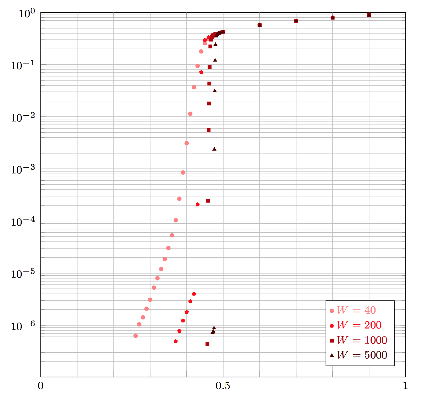
Figure 3: $n=6$ and $W\in\{40,200,1000,5000\}$.

The cases $n\in\{8,10\}$ and $W\in\{1000,5000\}$ are shown in Figure  4. Note that in order to see the error floor in this case one would have to simulate the curves to considerably lower probabilities since even for $n=8$ and $k=4$ we have already $\lceil 3^{4}/\sqrt{8}\rceil=29$. We see that compared to the case $n=6$ the threshold is even closer to the Shannon capacity, consistent with the threshold saturation phenomenon.

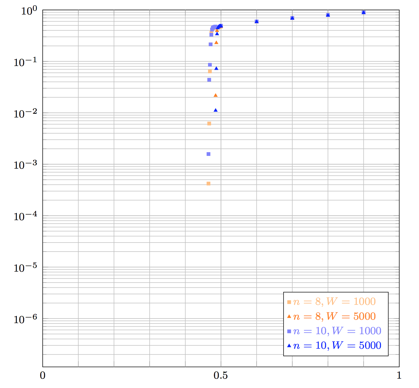
Figure 4: $n\in\{8,10\}$ and $W\in\{1000,5000\}$.

VI Conclusions

We introduced time-invariant low-density convolutional codes. These codes are defined by a very small number of bits. We have seen that despite their simplicity these codes perform very well. We have given some simple lower bound on the minimum stopping set size of such codes which grows exponentially in the number of shift-invariant parity-checks.

References

- [1] A. J. Felström and K. S. Zigangirov, “Time-varying periodic convolutional codes with low-density parity-check matrix,” IEEE Trans. Inform. Theory, vol. 45, no. 6, pp. 2181–2190, Sept. 1999.
- [2] M. Lentmaier, A. Sridharan, K. S. Zigangirov, and J. D. J. Costello, “Iterative decoding threshold analysis for LDPC convolutional codes,” IEEE Trans. Inform. Theory, vol. 56, no. 10, pp. 5274–5289, Oct. 2010.
- [3] S. Kudekar, T. Richardson, and R. Urbanke, “Threshold saturation via spatial coupling: Why convolutional ldpc ensembles perform so well over the bec,” in 2010 IEEE International Symposium on Information Theory, June 2010, pp. 684–688.
- [4] A. Yedla, Y. Y. Jian, P. S. Nguyen, and H. D. Pfister, “A simple proof of Maxwell saturation for coupled scalar recursions,” IEEE Transactions on Information Theory, vol. 60, no. 11, pp. 6943–6965, Nov 2014.
- [5] M. Luby, M. Mitzenmacher, A. Shokrollahi, D. A. Spielman, and V. Stemann, “Practical loss-resilient codes,” in Proc. of the 29th annual ACM Symposium on Theory of Computing, 1997, pp. 150–159.
- [6] T. Richardson, A. Shokrollahi, and R. Urbanke, “Design of capacity-approaching irregular low-density parity-check codes,” IEEE Trans. Inform. Theory, vol. 47, no. 2, pp. 619–637, Feb. 2001.
- [7] R. M. Tanner, “A recursive approach to low complexity codes,” IEEE Trans. Inform. Theory, vol. 27, no. 5, pp. 533–547, Sept. 1981.
- [8] A. J. Viterbi and J. K. Omura, Principles of Digital Communication and Coding. McGraw-Hill, 1979.
- [9] R. G. Gallager, “Low-density parity-check codes,” IRE Trans. Inform. Theory, vol. 8, pp. 21–28, Jan. 1962.
- [10] C. Berrou, A. Glavieux, and P. Thitimajshima, “Near Shannon limit error-correcting coding and decoding,” in Proc. of the IEEE Int. Conf. Commun. (ICC), Geneve, Switzerland, May 1993, pp. 1064–1070.
- [11] T. Richardson and R. Urbanke, Modern Coding Theory. Cambridge University Press, 2008.
- [12] C. Méasson, A. Montanari, and R. Urbanke, “Maxwell’s construction: The hidden bridge between maximum-likelihood and iterative decoding,” in Proc. of the IEEE Int. Symposium on Inform. Theory (ISIT), Chicago, 2004, p. 225.
- [13] C. Di, D. Proietti, T. Richardson, E. Telatar, and R. Urbanke, “Finite length analysis of low-density parity-check codes on the binary erasure channel,” IEEE Trans. Inform. Theory, vol. 48, pp. 1570–1579, Jun. 2002.