Theory of antiferromagnetic Heisenberg spins on breathing pyrochlore lattice

Abstract

Spin-singlet orders are studied for the antiferromagnetic Heisenberg model with spin $S>\frac{1}{2}$ on a breathing pyrochlore lattice, where tetrahedron units are weakly coupled and exchange constants have two values $0<J^{\prime}\ll J$. The ground state has a thermodynamic degeneracy at $J=0$, and I have studied lattice symmetry breaking associated to lifting this degeneracy. Third-order perturbation in $J^{\prime}$ for general spin $S$ shows that the effective Hamiltonian has a form of three-tetrahedron interactions of pseudospins $\bm{\tau}$, which is identical to that previously derived for $S=\frac{1}{2}$, and I have calculated their matrix elements for general $S$. For this effective Hamiltonian, I have obtained its mean-field ground state and investigated the possibility of lattice symmetry breaking for the cases of $S$=$\frac{3}{2}$ and 1. In contrast to the $S$=$\frac{1}{2}$ case, $\bm{\tau}$’s response to conjugate field has a $Z_{3}$ anisotropy in its internal space, and this stabilizes the mean-field ground state. The mean-field ground state has a characteristic spatial pattern of spin correlations related to the lattice symmetry breaking. Spin structure factor $S(\mathbf{q})$ is calculated and found to have symmetry broken parts with amplitudes of the same order as the isotropic part.

171 Frustration

1 Introduction

Frustrated magnets are a playground of the experimental and theoretical studies for the quest of new quantum phases FM1 ; FM2 . Thermodynamic degeneracy of the classical ground-state manifold is the most important ingredient, and the question is how this degeneracy is lifted to select a unique quantum ground state if it exists. Several cases still select some types orders of magnetic dipole moments despite frustration effects, but there also exist three other cases from the viewpoint of symmetry breaking: (i) Spin rotation symmetry is broken, but the order parameter is not a conventional magnetic dipole but something more exotic like quadrupole or vector chirality. (ii) While spin rotation symmetry is not broken, another type of symmetry is broken like lattice symmetry. (iii) No symmetry is broken: this case corresponds to a spin liquid but the liquid behavior does not determine if spin gap is finite or zero. Valence bond crystal (VBC) state Sachdev ; Lhuillier is a representative example of the case (ii), and the lattice rotation and/or translation symmetry is broken. Affleck-Kennedy-Lieb-Tasaki (AKLT) state AKLT is an example of the case (iii) and the spin gap is finite.

Generally speaking, exotic quantum phases are stabilized in frustrated magnets, if the frustration is strong enough and also if quantum fluctuations are large enough. The first condition is related to lattice geometry, and the Kagomé and pyrochlore lattices are the most typical examples in dimensions two and three, respectively. As for the second condition, factors enhancing quantum fluctuations include a high symmetry of the Hamiltonian, a low spatial dimensionality, and a small value of spin $S$.

The antiferromagnetic Heisenberg model on the pyrochlore lattice is a canonical example of frustrated quantum systems in three dimensions Reimers ; Harris ; Canals ; Yamashita ; Koga ; Tsunetsugu1 ; Tsunetsugu2 ; Henley . This lattice is a network of corner-sharing tetrahedron units, and thus each unit is highly frustrated. The pioneering mean-field analysis Reimers showed a huge degeneracy of the semiclassical ground-state manifold, manifested by the presence of zero-energy excitations in all over the Brillouin zone Tsunetsugu3 . Over a decade ago I studied the quantum limit $S$=$\frac{1}{2}$ of this model and examined the possibility of exotic orders like scalar chirality Tsunetsugu1 . This expectation came from the fact that the doubly degenerate ground states in each tetrahedron unit have opposite scalar chiralities. I derived an effective Hamiltonian in the subspace where every tetrahedron unit is within the two-dimensional local ground-state multiplet of spin singlet and analyzed that Hamiltonian. The result showed that the ground state does not have a scalar chirality order but it is a mixture of local singlet dimers and/or tetramers and thus the lattice symmetry is broken Tsunetsugu1 ; Tsunetsugu2 . The spatial pattern of these dimers/tetramers is quite complicated and this is due to frustration in their configuration. Three-quarters of tetrahedron units have a specific favorable configuration of dimer pairs, but the remaining quarter of units have no favorable configuration. This is a frustration in the mean-field level, and quantum fluctuations select a uniform order of either dimer pairs or tetramers in the remaining part Tsunetsugu2 .

In my previous study for the $S$=$\frac{1}{2}$ case, I introduced one parameter for controlling geometrical frustration. The original pyrochlore lattice was split into two parts: one is the set of pointing-up tetrahedron units and the other is the set of bonds connecting these units. The control parameter is the ratio of exchange constants for the two parts $J^{\prime}/J$, and I approached the original model ($J^{\prime}/J$=1) by perturbation starting from the decoupled limit $J^{\prime}/J$=0 Tsunetsugu1 ; Tsunetsugu2 . A different split was also examined by another group Koga but my split had the advantage of keeping the tetrahedral lattice symmetry.

A few years ago, Okamoto et al. Okamoto1 noticed that Cr ions in the compounds LiGa_1-xIn_xCr₄O₈ ($0\leq x\leq 1$) constitute a network corresponding to my previous perturbative expansion and named this sublattice breathing pyrochlore. Despite the same lattice structure, this system differs from my previous model in the point that Cr ions have spin $S$=$\frac{3}{2}$. The In end ($x=1$) has largest breathing and shows an antiferromagnetic phase transition at the temperature $T_{N}$=13-14 K Tanaka ; Okamoto2 . This is much smaller compared with the modulus of the Weiss temperature $|\theta_{W}|$=332 K, showing the effects of frustration. This magnetic phase is very fragile against reducing In-ion concentration, disappearing at around $x\sim 0.9$, and the system remains paramagnetic down to the lowest temperature 2 K. This may indicate that nonmagnetic ground state is stabilized in the breathing pyrochlore lattice. Therefore, it is interesting to reinvestigate the problem now for the case of $S$=$\frac{3}{2}$ and also for general $S$, and I will examine how the results depend on $S$. It will turn out that for $S>\frac{1}{2}$ there appears a generic anisotropy in dimer/tetramer configuration and this stabilizes a specific spatial modulation of spin correlations. This will be manifested in the wave-vector dependence of the energy-integrated spin structure factor $S(\mathbf{q})$, and I will calculate its explicit form.

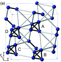
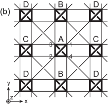
Figure 1: (a) Cubic unit cell of breathing pyrochlore lattice. Tetrahedron units made of short bonds (black) with strong $J$ are connected by long bonds (gray) with weak $J^{\prime}$. A-D are the sublattice labels of the tetrahedron units. (b) A slice of breathing pyrochlore lattice projected onto the $xy$-plane. The parts shown by thick lines are tetrahedron units. The layer of the units A and D is located above that of B and C in this part. Numbers 1-4 are the site labels in each tetrahedron unit.

2 Model

In this paper, I study the ground state of a spin-$S$ Heisenberg model on a breathing pyrochlore lattice, and apply the results to the $S=\frac{3}{2}$ case, which may be realized in the Cr compound Li$X$Cr₄O₈. The original pyrochlore lattice is a network of two types of corner-sharing tetrahedra, and they have the same size. In breathing pyrochlore lattice, one type of tetrahedra expand in size and the other type shrink, but neither of them change their shape of regular tetrahedron. See Fig. 1(a). The Hamiltonian to study is a spin-$S$ Heisenberg model with antiferromagnetic interactions between nearest neighbor sites on the breathing pyrochlore lattice, and I will analyze the cases of $S=\frac{3}{2}$ and 1 in detail. Exchange coupling has two values depending on bond length in the breathing lattice structure

$$H =J\sum_{\mathbf{r}}\sum_{1\leq i<j\leq 4}\!\!\mathbf{S}_{i}(\mathbf{r})\cdot\mathbf{S}_{j}(\mathbf{r})+J^{\prime}\sum_{\langle(i,\mathbf{r}),(j,\mathbf{r}^{\prime})\rangle}\!\!\!\!\mathbf{S}_{i}(\mathbf{r})\cdot\mathbf{S}_{j}(\mathbf{r}^{\prime})$$ (1a)

$$=\sum_{\mathbf{r}}H_{\mathrm{unit}}(\mathbf{r})+\sum_{\langle\mathbf{r},\mathbf{r}^{\prime}\rangle}H_{1}(\mathbf{r},\mathbf{r}^{\prime}),$$ (1b)

where $\mathbf{r}$ denotes the position of small tetrahedron and $i,j$ are the site labels as shown in Fig. 1(b). Six bonds in each small tetrahedron unit have strong interaction $J>0$, while the units are coupled by long bonds with weak antiferromagnetic interaction $0<J^{\prime}(\ll J)$. In the following, I will call small tetrahedra with strong bonds tetrahedron units, and then they are connected by weak bonds in large tetrahedra. Throughout this paper, I use $N$ to denote the number of spins, and then the number of tetrahedron units is $\frac{1}{4}N$. Note that the Hamiltonian is invariant upon exchanging $J$ and $J^{\prime}$ due to the lattice symmetry.

I studied in Refs. Tsunetsugu1 ; Tsunetsugu2 this model for the $S=\frac{1}{2}$ case and discovered a complex pattern of spin dimers and tetramers in the ground state. I will later focus on the special cases of $S=\frac{3}{2}$ and $S=1$ afterwards, but first study this Hamiltonian for general $S$ to compare the cases of different spin quantum numbers $S$.

3 Spin singlet states in one tetrahedron unit

Following Refs. Tsunetsugu1 ; Tsunetsugu2 , I employ an approach of degenerate perturbation in $J^{\prime}/J$. The first step is to understand eigenstates in the limit of decoupled tetrahedra ($J^{\prime}$=0). The Hamiltonian of a single tetrahedron unit at position $\mathbf{r}$ is

$$H_{\mathrm{unit}}(\mathbf{r})=J\!\sum_{1\leq i<j\leq 4}\mathbf{S}_{i}(\mathbf{r})\cdot\mathbf{S}_{j}(\mathbf{r})=J[{\textstyle\frac{1}{2}}\,\mathbf{S}_{\mathrm{unit}}^{2}(\mathbf{r})-2S(S+1)].$$ (2)

Here, $\mathbf{S}_{\mathrm{unit}}(\mathbf{r})=\sum_{i=1}^{4}\mathbf{S}_{i}(\mathbf{r})$ is the total spin of this unit and its quantum number is an integer $0\leq S_{\mathrm{unit}}\leq 4S$. Therefore, the eigenenergies of $H_{\mathrm{unit}}(\mathbf{r})$ are determined by the unit spin alone as $E_{\mathrm{unit}}=J[{\textstyle\frac{1}{2}}\,S_{\mathrm{unit}}(S_{\mathrm{unit}}+1)-2S(S+1)]$ and the ground-state manifold coincides with the entire space of $S_{\mathrm{unit}}$=0. These results have been well-known including the fact that the ground states in each unit have degeneracy $2S+1$, and thus the ground-state degeneracy in the entire system is $(2S+1)^{N/4}$ where $N$ is the number of original spins Tsunetsugu1 . This corresponds to the residual entropy that is precisely 25% of the total entropy irrespective of the value of $S$.

The issue of this study is how the weak inter-unit interactions $J^{\prime}$ release the macroscopic entropy and which type of ground state is selected. Since anything interesting happens in the spin-singlet space, the spin rotation symmetry has no chance to be broken, and it is the lattice symmetry that can be broken. To examine this issue, symmetry argument is useful and I will check how the $(2S+1)$-fold ground states in each unit are transformed with operations of the point group symmetry. Each unit has the tetrahedral symmetry $T_{d}$, and this point group has 5 types of irreducible representations (irreps) group : 2 one-dimensional ones (A₁ and A₂), 1 two-dimensional one (E), and 2 three-dimensional ones (T₁ and T₂).

To perform calculation, we need an explicit form of $(2S+1)$-states in the space of $S_{\mathrm{unit}}=0$. A convenient choice is the following one

$$\Phi_{l}=\sum_{l_{z}=-l}^{l}C(l,l_{z})\phi^{(12)}(l,l_{z})\otimes\phi^{(34)}(l,-l_{z}),\ \ \mathbf{S}_{\mathrm{unit}}^{2}\Phi_{l}=0,$$ (3)

where $l$ is an integer satisfying $0\,$$\leq$$\,l$$\,\leq$$\,2S$. Here, $\phi^{(12)}(l,l_{z})$ is the wavefunction in which the two spins $\mathbf{S}_{1}$ and $\mathbf{S}_{2}$ couple to form a state with the composite spin $l$ and its $z$-projection $l_{z}$, while the remaining two spins $\mathbf{S}_{3}$ and $\mathbf{S}_{4}$ do the same in $\phi^{(34)}(l,-l_{z})$ but with the opposite $z$-projection. These two-spin wavefunctions are written with single-spin bases as

$$\phi^{(ij)}(l,l_{z})=\sum_{m=\max\{-S,l_{z}-S\}}^{\min\{S,l_{z}+S\}}\langle S,S,m,l_{z}-m|l,l_{z}\rangle|S,m\rangle_{i}\otimes|S,l_{z}-m\rangle_{j},$$ (4)

where $\langle S,S,m,l_{z}-m|l,l_{z}\rangle$ is the Clebsch-Gordan (CG) coefficient of combining two angular momenta Messiah , and these wavefunctions have the symmetry

$$\phi^{(ji)}(l,l_{z})=(-1)^{2S+l}\phi^{(ij)}(l,l_{z}).$$ (5)

These two composite spins couple and finally form a total spin singlet in a tetrahedron unit. The prefactor $C$ in Eq. (3) is also given by a CG coefficient and this is simple because the total spin is singlet

$$C(l,l_{z})=\langle l,l,l_{z},-l_{z}|0,0\rangle=\frac{(-1)^{l-l_{z}}}{\sqrt{2l+1}}=C(l,-l_{z}).$$ (6)

These $(2S+1)$ wavefunctions $\{\Phi_{l}\}$ constitute a complete orthonormal set in the $S_{\mathrm{unit}}$=0 space at each tetrahedron unit.

I have classified these $\Phi_{l}$’s according to the $T_{d}$ point group symmetry. This was done by calculating the characters of the symmetry operations, and the details of calculation are explained in Appendix A. The result turns out interesting. For any value of individual spin $S$, all of the $2S+1$ ground states in the tetrahedron unit belong to $A_{1}$, $A_{2}$, and $E$ irreps, while no ground states transform as the three-dimensional irrep $T_{1}$ or $T_{2}$. I have calculated the multiplicity of these irreps and the result is $\bigl{\{}\Phi_{l}\bigr{\}}_{l=0}^{2S}=n_{1+}A_{1}\oplus n_{1-}A_{2}\oplus n_{2}E$ with

$$n_{1\pm}={\textstyle\frac{1}{6}}(2S+1\pm 3\chi_{2}+2\chi_{5}),\ n_{2}={\textstyle\frac{1}{3}}(2S+1-\chi_{5}).$$ (7)

Here, $\chi_{2}$=$\mbox{mod }(2S-1,2)$ and $\chi_{5}$=$\mbox{mod }(2S-1,3)-1$.

4 Effective Hamiltonian for general $S$

Now, I am going to derive an effective Hamiltonian that lifts the macroscopic degeneracy of the ground states in the limit of decoupled tetrahedra. To this end, one needs a degenerate perturbation in the weak interaction $J^{\prime}$, and I succeeded in this task for the $S=\frac{1}{2}$ case after a lengthy calculation of many matrix elements Tsunetsugu1 ; Tsunetsugu2 . For larger spins, the local Hilbert space increases its dimension, and this makes calculations more impracticable and difficult. Therefore, I took a different strategy and tried to simplify the formulation in perturbation as much as possible. I have achieved a huge simplification in the third-order perturbation, and this works for any value of spin $S$. With this simplified formulation, my previous result for the $S=\frac{1}{2}$ case is also easily reproduced.

The effective Hamiltonian is to be derived for describing dynamics in the low-energy subspace where all the local states at tetrahedron units are within the spin-singlet manifold, and let me comment on its validity. The use of such an effective Hamiltonian is justified under two conditions. The first condition is the presence of a finite spin gap $\Delta_{s}>0$. The size of the spin gap depends on the ratio of two exchange constants, $\Delta_{s}=J\bar{\Delta}(\frac{J^{\prime}}{J};S)$ with $\bar{\Delta}(0;S)=1$, and the first condition is satisfied at least for small $\frac{J^{\prime}}{J}$. The second condition is that the energy range of consideration should be smaller than the spin gap, $\varDelta E<\Delta_{s}$, where $\varDelta E$ is measured from the ground-state energy. For studying the high-energy region $\varDelta E>\Delta_{s}$, it is necessary to take account of the subspaces with $S_{\mathrm{unit}}\geq 1$ on the same footing as the $S_{\mathrm{unit}}=0$ subspace, which is beyond the approximation of this effective Hamiltonian.

Before demonstrating how perturbation calculation is simplified, I now introduce matrix elements necessary for that and discuss their symmetry. They are two-spin correlations defined for a pair of ground states in one tetrahedron unit

$$\langle\Phi_{\alpha}|S_{i}^{\mu}S_{j}^{\nu}|\Phi_{\beta}\rangle={\textstyle\frac{1}{3}}\delta_{\mu\nu}f_{\alpha\beta}^{(ij)},\ \ f_{\alpha\beta}^{(ij)}=\langle\Phi_{\alpha}|\mathbf{S}_{i}\cdot\mathbf{S}_{j}|\Phi_{\beta}\rangle,$$ (8)

Here, $\mu,\nu\in\{x,y,z\}$ are spin index, and the result is diagonal in spin space because spin-singlet states are rotationally invariant. For the same site correlation, it is trivial, simply $f_{\alpha\beta}^{(ii)}$=$S(S+1)\langle\Phi_{\alpha}|\Phi_{\beta}\rangle$. Using the fact that the two states are both spin singlet, one can further prove important symmetries of $f^{(ij)}$ for $i$$\neq$$j$. For a site pair in a tetrahedron unit, let call the remaining two sites its conjugate site pair; e.g., for the site pair 1-2, its conjugate pair is 3-4. For the site pair $i$-$j$, let us define

$$f_{\alpha\beta}^{(ij)}=:-c_{0}\langle\Phi_{\alpha}|\Phi_{\beta}\rangle+\bigl{(}{\mathsf{F}}^{(ij)}\bigr{)}_{\alpha\beta},\ \ c_{0}={\textstyle\frac{1}{3}}S(S+1),$$ (9)

and then $\mathsf{F}^{(ij)}$ is identical to the value for its conjugate site pair:

$${\mathsf{F}}^{(12)}={\mathsf{F}}^{(34)},\ {\mathsf{F}}^{(13)}={\mathsf{F}}^{(24)},\ {\mathsf{F}}^{(14)}={\mathsf{F}}^{(23)},$$ (10)

and the sum of these vanish

$${\mathsf{F}}^{(12)}+{\mathsf{F}}^{(13)}+{\mathsf{F}}^{(14)}=0.$$ (11)

These $\mathsf{F}$’s are a square matrix with dimension $2S+1$. These relations (10) and (11) will be referred to in the following as conjugate-pair equivalence and neutrality identity, respectively.

Before going to perturbation calculations, I quickly prove Eqs. (10) and (11). For the conjugate-pair equivalence, it is sufficient to prove $f_{\alpha\beta}^{(12)}$=$f_{\alpha\beta}^{(34)}$, and the following proof does not depend on the choice of site pair $i$-$j$. Let $\mathbf{S}_{\mathrm{unit}}$ be the total spin in the tetrahedron unit, $\mathbf{S}_{\mathrm{unit}}$=$\sum_{i=1}^{4}\mathbf{S}_{i}$, and here I drop the label of the unit position $\mathbf{r}$, since all the calculations are limited in one unit. For any tetrahedron singlet state $\Phi_{\alpha}$, the most important relation is

$$\mathbf{S}_{\mathrm{unit}}|\Phi_{\alpha}\rangle=\mathbf{0},\ \ \langle\Phi_{\alpha}|\mathbf{S}_{\mathrm{unit}}=\mathbf{0}.$$ (12)

Another relation to use is the identity $\mathbf{S}_{i}\cdot\mathbf{S}_{j}=\frac{1}{2}\mathbf{S}_{ij}^{2}-S(S+1)$, where $\mathbf{S}_{ij}\equiv\mathbf{S}_{i}+\mathbf{S}_{j}$ is the composite spin of the pair. Then, the relation to prove is equivalent to

$$\langle\Phi_{\alpha}|\mathbf{S}_{12}^{2}|\Phi_{\beta}\rangle=\langle\Phi_{\alpha}|\mathbf{S}_{34}^{2}|\Phi_{\beta}\rangle.$$ (13)

Using $\mathbf{S}_{\mathrm{unit}}$, the 3-4 site pair can be represented by quantities related to the 1-2 site pair

$$\langle\Phi_{\alpha}|\mathbf{S}_{34}^{2}|\Phi_{\beta}\rangle=\langle\Phi_{\alpha}|(\mathbf{S}_{\mathrm{unit}}-\mathbf{S}_{12})\cdot(\mathbf{S}_{\mathrm{unit}}-\mathbf{S}_{12})|\Phi_{\beta}\rangle=\langle\Phi_{\alpha}|\mathbf{S}_{12}^{2}|\Phi_{\beta}\rangle.$$ (14)

This completes the proof of the conjugate-pair equivalence.

Using the conjugate-pair equivalence for three pairs, one can rewrite the neutrality identity as follows

$$\Bigl{\langle}\Phi_{\alpha}\Big{|}S(S+1)+{\textstyle\frac{1}{2}}\sum_{1\leq i<j\leq 4}\mathbf{S}_{i}\cdot\mathbf{S}_{j}\Big{|}\Phi_{\beta}\Bigr{\rangle}=0.$$ (15)

It is straightforward to prove this, since the left-hand side is nothing but $\langle\Phi_{\alpha}|\frac{1}{4}\mathbf{S}_{\mathrm{unit}}^{2}|\Phi_{\beta}\rangle$=0. Thus, the neutrality identity is also proved.

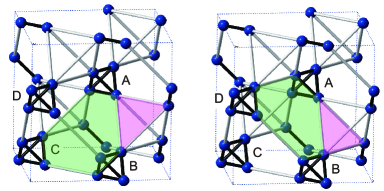
Figure 2: Two types of paths appearing in the third-order perturbation. Shown are 2 pairs of hexagon and triangular loops that share the same long bond connecting A and B units. Each loop contains 3 long bonds.

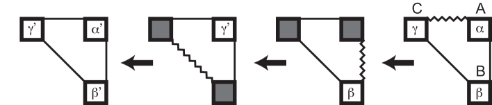
Figure 3: One process in the third-order perturbation for the tetrahedron units $A$-$C$. This starts from the product state of three singlets $\big{|}\Phi_{\alpha}^{A}\Phi_{\beta}^{B}\Phi_{\gamma}^{C}\bigr{\rangle}$, and each zigzag bond depicts a perturbation $J^{\prime}S_{i}(\mathbf{r})\cdot S_{j}(\mathbf{r}^{\prime})$ to be operated. Shadowed units are tetrahedra excited to $S_{\mathrm{unit}}$=1, while all the others remain in $S_{\mathrm{unit}}$=0. Different orders of operating three perturbations generate 5 other processes, and all of them have the same contribution as the process shown here, since the three perturbations commute to each other.

We are now ready to start a degenerate perturbation for constructing an effective Hamiltonian. In perturbation in $J^{\prime}$, first-order terms vanish and second-order terms only yield a constant energy shift for all states

$$\varDelta E_{0}^{(2)}=-\frac{J^{\prime 2}}{6J}\bigl{[}S(S+1)\bigr{]}^{2}\times\frac{3}{2}N,$$ (16)

where $\frac{3}{2}N$ is the total number of long bonds. Therefore, the leading terms that lift the degeneracy are third order ones, which was explicitly derived for the $S=\frac{1}{2}$ case Tsunetsugu1 . Beware that there are two types of third-order terms. One corresponds to perturbation paths on triangular loops made of weak bonds alone, and they contribute only a constant energy shift again,

$$\varDelta E_{0}^{(3)}=\frac{J^{\prime 3}}{6J^{2}}\bigl{[}S(S+1)\bigr{]}^{3}\times N,$$ (17)

where $N$ should be read as the number of the triangular loops, which is identical to the number of original spins.

The other type is what we need and corresponds to perturbation paths on hexagon loops each of which includes three weak bonds. Two examples of the latter type are shown in Fig. 2. The colored hexagon loop in the left panel includes the three tetrahedron units $ABC$ and the corresponding third-order perturbation term is given by

$$\bigl{\langle}\Phi_{\alpha^{\prime}}^{A}\Phi_{\beta^{\prime}}^{B}\Phi_{\gamma^{\prime}}^{C}\big{|}H_{\mathrm{eff}}(ABC)\big{|}\Phi_{\alpha}^{A}\Phi_{\beta}^{B}\Phi_{\gamma}^{C}\bigr{\rangle}$$

$$={3!J^{\prime 3}}\sum_{v_{1},v_{2}}\frac{\bigl{\langle}\Phi_{\alpha^{\prime}}^{A}\Phi_{\beta^{\prime}}^{B}\Phi_{\gamma^{\prime}}^{C}\big{|}\mathbf{S}_{4}(A)\cdot\mathbf{S}_{1}(B)\big{|}v_{2}\bigr{\rangle}\bigl{\langle}v_{2}\big{|}\mathbf{S}_{3}(B)\cdot\mathbf{S}_{4}(C)\big{|}v_{1}\bigr{\rangle}}{\varDelta\varepsilon_{ABC}(v_{2})\,\varDelta\varepsilon_{ABC}(v_{1})}$$

$$\hskip 113.81102pt\times\bigl{\langle}v_{1}\big{|}\mathbf{S}_{1}(C)\cdot\mathbf{S}_{3}(A)\big{|}\Phi_{\alpha}^{A}\Phi_{\beta}^{B}\Phi_{\gamma}^{C}\bigr{\rangle}$$ (18a)

$$=\frac{3!J^{\prime 3}}{(2J)^{2}}\Bigl{\langle}\Phi_{\alpha^{\prime}}^{A}\Phi_{\beta^{\prime}}^{B}\Phi_{\gamma^{\prime}}^{C}\Big{|}[\mathbf{S}_{4}(A)\cdot\mathbf{S}_{1}(B)][\mathbf{S}_{3}(B)\cdot\mathbf{S}_{4}(C)][\mathbf{S}_{1}(C)\cdot\mathbf{S}_{3}(A)]\Big{|}\Phi_{\alpha}^{A}\Phi_{\beta}^{B}\Phi_{\gamma}^{C}\Bigr{\rangle}$$ (18b)

$$=\frac{3!J^{\prime 3}}{(2J)^{2}}\sum_{\mu_{1},\mu_{2},\mu_{3}}\Bigl{[}\bigl{\langle}\Phi_{\alpha^{\prime}}\big{|}{S}_{4}^{\mu_{1}}{S}_{3}^{\mu_{3}}\big{|}\Phi_{\alpha}\bigr{\rangle}\Bigr{]}_{A}\Bigl{[}\bigl{\langle}\Phi_{\beta^{\prime}}\big{|}{S}_{1}^{\mu_{1}}{S}_{3}^{\mu_{2}}\big{|}\Phi_{\beta}\bigr{\rangle}\Bigr{]}_{B}\Bigl{[}\bigl{\langle}\Phi_{\gamma^{\prime}}\big{|}{S}_{4}^{\mu_{2}}{S}_{1}^{\mu_{3}}\big{|}\Phi_{\gamma}\bigr{\rangle}\Bigr{]}_{C}$$ (18c)

$$=\frac{J^{\prime 3}}{6J^{2}}\,{f}^{(12)}_{A,\alpha^{\prime}\alpha}\,{f}^{(13)}_{B,\beta^{\prime}\beta}\,{f}^{(14)}_{C,\gamma^{\prime}\gamma},$$ (18d)

where $v$’s are excited states of the system of the units $ABC$ and $\varDelta\varepsilon_{ABC}(v)$ is their excitation energy measured from the ground state value. Note that the conjugate-pair equivalence has been used for the unit $A$, $f^{(34)}=f^{(12)}$. One process is depicted in Fig. 3 and this corresponds to the matrix elements in Eq. (18a). The factor $3!$ comes from the fact that different orders of three $\mathbf{S}\cdot\mathbf{S}$’s have all the same contribution. The sums $\sum_{v_{1},v_{2}}$ are originally taken over all the excited states of the units $ABC$, but matrix elements are nonvanishing only with those $v$’s in which two units are excited to $S_{\mathrm{unit}}$=1 and one unit remains $S_{\mathrm{unit}}$=0. Therefore, the excitation energy is always $\varDelta\epsilon_{ABC}(v)$=$2J$ for any of those $v$, and one can move the energy denominators to outside the sum. I should emphasize that this is a special feature of the present model, and this simplifies calculations. After doing this, one can modify the sum $\sum_{v_{1},v_{2}}$ now with including the ground states. This modification does not change the result, because the additionally included ground states have only zero matrix elements. The modified sum for the virtual states is taken over the entire Hilbert space of the three units, and therefore we can safely drop this sum, $(\sum_{\mathrm{excited\ states}}+\sum_{\mathrm{ground\ states}})|v\rangle\langle v|=1$. Thus, Eq. (18b) is obtained, and it is straightforward to rewrite that into the final step (18d). There, the unit index $A$-$C$ is added in the subscript to show explicitly which unit contributes to each $f$ factor.

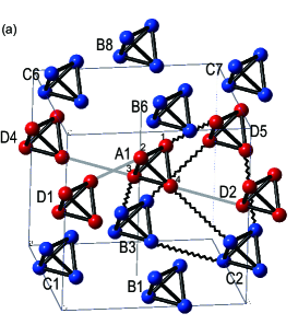
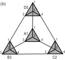
Figure 4: (a) Network of effective interactions. Since tetrahedron units form a face center cubic lattice, each unit is surrounded by 12 nearest neighbors. The number accompanying $A$-$D$ is the label of cubic unit cell. The central unit $A$1 is surrounded by 4 $D$-units in the same layer, and 4 $B$- and also 4 $C$-units in the layer either below or above. Long bonds connecting $A$ and $D$’s are also shown. Setting one of its vertices as an apex, each unit form a quartet of tetrahedron units together with three neighbors. Shown with zigzag lines is the case where the apex is the site 2 of the unit $A$1. This quartet has three hexagon loops that attach the $A$1 unit, and each loop corresponds to one term in the effective Hamiltonian (22). Therefore, the Hamiltonian has 12 terms containing $\bm{\tau}_{A1}$. (b) Connectivity of 4 units in the tetrahedron quartet selected in (a). The numbers 1-4 are site index in each unit.

The neutrality identity implies that only two of the operators $\mathsf{F}^{(1j)}$’s are independent in each tetrahedron unit, and I choose the following two

$$\tau_{1}=\mathsf{F}^{(12)},\ \ \tau_{2}={\textstyle\frac{1}{\sqrt{3}}}(\mathsf{F}^{(13)}-\mathsf{F}^{(14)}).$$ (19)

I have checked that these operators transform as basis of the $E$-irrep upon operations in the $T_{d}$ point group, and

$$\mathsf{F}^{(12)}=\mathbf{e}_{0}\cdot\bm{\tau},\ \ \mathsf{F}^{(13)}=\mathbf{e}_{1}\cdot\bm{\tau},\ \ \mathsf{F}^{(14)}=\mathbf{e}_{2}\cdot\bm{\tau},\ \$$ (20)

with $\mathbf{e}_{m}=\mathbf{e}(\mbox{$\theta$=$2m\pi/3$})$ where $\mathbf{e}(\theta)=(\cos\theta,\sin\theta)$. As will be shown in Eq. (28) and Appendix B, all of the operators $\{\mathsf{F}^{1j}\}$ have eigenvalues

$$\lambda_{l}=-{\textstyle\frac{2}{3}}S(S+1)+{\textstyle\frac{1}{2}}l(l+1),\ \ \ (l\in\{0,1,\cdots,2S\}).$$ (21)

The full effective Hamiltonian in the third order is obtained by repeating the same calculation for all the tetrahedron triads participating to the shortest hexagon loops in the breathing pyrochlore lattice. With these new operators $\bm{\tau}$, the effective Hamiltonian for the spin-$S$ Heisenberg model (1b) is represented as

$$H_{\mathrm{eff}}=-J_{\mathrm{eff}}\!\!\!\!\!\sum_{\langle\mathbf{r},\mathbf{r}^{\prime},\mathbf{r}^{\prime\prime}\rangle}\!\!\bigl{(}c_{0}-\mathbf{e}_{0}\cdot\bm{\tau}_{\mathbf{r}}\bigr{)}\bigl{(}c_{0}-\mathbf{e}_{1}\cdot\bm{\tau}_{\mathbf{r}^{\prime}}\bigr{)}\bigl{(}c_{0}-\mathbf{e}_{2}\cdot\bm{\tau}_{\mathbf{r}^{\prime\prime}}\bigr{)},$$ (22)

where the parameters are

$$J_{\mathrm{eff}}=\frac{J}{6}\left(\frac{J^{\prime}}{J}\right)^{3}>0,\hskip 14.22636ptc_{0}={\textstyle\frac{1}{3}}S(S+1).$$ (23)

Here the sum is taken over all the tetrahedron triads explained before. As explained in the caption of Fig. 4, the number of terms in $H_{\mathrm{eff}}$ is $12\times\frac{1}{4}N\times\frac{1}{3}=N$, where $N$ is the number of original spins and the factor $\frac{1}{3}$ comes from the fact that each term of this three-unit interaction is counted three times. Corresponding to the choice of three units out of the four sublattices $A$-$D$, $H_{\mathrm{eff}}$ has 4 types of terms and the prefactors $\mathbf{e}_{m}$’s in Eq. (22) should be chosen as follows depending on sublattices

$$\begin{array}[]{cccc}&\ \ \mathbf{e}_{0}&\ \ \mathbf{e}_{1}&\ \ \mathbf{e}_{2}\\ \hline\cr\mbox{type }(1)&A&B&C\\ \phantom{\mbox{type }}(2)&B&A&D\\ \phantom{\mbox{type }}(3)&C&D&A\\ \phantom{\mbox{type }}(4)&D&C&B\\ \hline\cr\end{array}$$ (24)

One should note that each $\mathbf{e}_{m}$ appears once and only once in each triple product term in Eq. (22). The prefactor $\mathbf{e}_{m}$ is determined by how its tetrahedron unit is connected to the hexagon loop. It is $\mathbf{e}_{0}$ if the unit is connected with the site pair 1-2 or 3-4, $\mathbf{e}_{1}$ for 1-3 or 2-4, and $\mathbf{e}_{2}$ for 1-4 or 2-3.

This effective Hamiltonian derived for general $S$ is identical to the one obtained in the previous studies for the $S=\frac{1}{2}$ case Tsunetsugu1 ; Tsunetsugu2 . The only but essential difference is that $\bm{\tau}_{\mathbf{r}}$ now operates in the local singlet space which has the dimension $2S+1$. For $S=\frac{1}{2}$, $\bm{\tau}$ are a half of Pauli matrices and $c_{0}$=$\frac{1}{4}$, and the Hamiltonian  (22) reduces to the effective model in Refs. Tsunetsugu1 ; Tsunetsugu2 up to the numerical factors. Expanding the triple products in $H_{\mathrm{eff}}$, it is again found that all the terms linear in $\bm{\tau}$ vanish for any $S$.

Before proceeding to the next step, I briefly comment on the classical limit $S=\infty$, and explain that the present perturbative approach fails there. With increasing $S$ to infinity, while the quantum Hamiltonian converges to the classical Heisenberg model, the quantum ground state does not continuously evolve to the ground state of the classical model. The reason is the following.

As explained at the beginning of this section, the use of the effective Hamiltonian is limited to the ground state and the low-energy sector of the original Heisenberg model where the excitation energy is smaller than the spin gap $\varDelta E<\Delta_{s}=J\bar{\Delta}_{s}(\frac{J^{\prime}}{J};S)$. In the $S=\infty$ limit, the classical Heisenberg model is defined with classical unit vectors $\mathbf{s}_{i}(\mathbf{r})$’s as $H_{\mathrm{cl}}=J_{\mathrm{cl}}\sum_{\mathbf{r},i<j}\mathbf{s}_{i}(\mathbf{r})\cdot\mathbf{s}_{j}(\mathbf{r})$ $+J^{\prime}_{\mathrm{cl}}\sum_{\langle(i,\mathbf{r}),(j,\mathbf{r}^{\prime})\rangle}\mathbf{s}_{i}(\mathbf{r})\cdot\mathbf{s}_{j}(\mathbf{r}^{\prime})$. To converge to this upon increasing $S$ in the quantum Hamiltonian (1a), one needs to renormalize spin variables as $\mathbf{S}_{i}(\mathbf{r})=S\mathbf{s}_{i}(\mathbf{r})$, and this requires a proper scaling of the exchange constants

$$J=\frac{J_{\mathrm{cl}}}{S^{2}},\ \ J^{\prime}=\frac{J^{\prime}_{\mathrm{cl}}}{S^{2}},$$ (25)

where $J_{\mathrm{cl}}$ and $J^{\prime}_{\mathrm{cl}}$ are constants independent of $S$. This immediately implies that $\varDelta E<\frac{J_{\mathrm{cl}}}{S^{2}}\bar{\Delta}_{s}(\frac{J^{\prime}_{\mathrm{cl}}}{J_{\mathrm{cl}}};S)\rightarrow 0$ with $S\rightarrow\infty$, and the energy region of the effective model shrinks to zero in the classical limit. Thus, the low-energy region of the quantum Hamiltonian (1a) with finite $S$ is not continuously connected to that in the classical Heisenberg model. In particular, the $S=\infty$ limit is a singular point for the ground state: the spin rotation symmetry is not broken in the ground state for any finite $S$, but it is broken in the classical ground state. Therefore, it is impossible to formulate an expansion of $\frac{1}{S}$ type starting from the classical limit. This contrasts with the case of magnetically ordered states, where the $\frac{1}{S}$-expansion correctly describes the ordered ground state and magnon excitations in the corresponding quantum system. The classical Heisenberg model on the pyrochlore lattice is itself exotic, and the ground state is thermodynamically degenerate Reimers ; Benton .

5 Spin-pair operators $\bm{\tau}$ for general $S$

To analyze the effective Hamiltonian, one needs to know an explicit form of $\bm{\tau}$ operators, and this is another challenge for $S>\frac{1}{2}$. In this section, I am going to calculate the matrix elements of $\bm{\tau}$ in terms of the basis states $\{\Phi_{l}\}$ defined in Eq. (3). It turns out useful to introduce uniform and staggered components of spin pair,

$$\mathbf{S}_{ij}\equiv\mathbf{S}_{i}+\mathbf{S}_{j},\ \ \mathbf{N}_{ij}\equiv\mathbf{S}_{i}-\mathbf{S}_{j},\ \$$ (26)

and their ladder operators, $S_{ij}^{\pm}\equiv S_{ij}^{x}\pm iS_{ij}^{y}$ and $N_{ij}^{\pm}\equiv N_{ij}^{x}\pm iN_{ij}^{y}$.

The spin-pair wavefunction $\phi^{(12)}(l,l_{z})$ is an eigenvector of $\mathbf{S}_{12}^{2}$ with the eigenvalue $l(l+1)$ for any $l_{z}$. Therefore, this is also the case for our basis functions in the $S_{\mathrm{unit}}=0$ subspace of tetrahedron unit, and

$$l(l+1)\Phi_{l}=\mathbf{S}_{12}^{2}\Phi_{l}=2\bigl{[}S(S+1)+\mathbf{S}_{1}\cdot\mathbf{S}_{2}\bigr{]}\Phi_{l}.$$ (27)

This immediately leads to the matrix elements of $\tau_{1}$

$$\bigl{(}\tau_{1}\bigr{)}_{l^{\prime}l}=F_{l^{\prime}l}^{(12)}=\langle\Phi_{l^{\prime}}|{\textstyle\frac{1}{3}}S(S+1)+\mathbf{S}_{1}\cdot\mathbf{S}_{2}|\Phi_{l}\rangle=\bigl{[}{\textstyle\frac{1}{2}}l(l+1)-{\textstyle\frac{2}{3}}S(S+1)\bigr{]}\delta_{l^{\prime}l}.$$ (28)

This matrix is diagonal and traceless, $\sum_{l=0}^{2S}(\tau_{1})_{ll}=0$. The largest and smallest eigenvalues are $\frac{1}{3}S(4S+1)$ and $-\frac{2}{3}S(S+1)$, respectively.

The calculation of $\tau_{2}=\frac{1}{\sqrt{3}}(\mathsf{F}^{(13)}-\mathsf{F}^{(14)})=\frac{1}{\sqrt{3}}(2\mathsf{F}^{(13)}-\mathsf{F}^{(12)})$ is more elaborate, since the operation of $\mathbf{S}_{1}\cdot\mathbf{S}_{3}$ or $\mathbf{S}_{1}\cdot\mathbf{S}_{4}$ hybridizes different $\Phi_{l}$’s and four-spin nature of the wavefunctions complicates its evaluation. As shown in Appendix B, $\mathsf{F}^{(13)}$ is related to $\mathsf{F}^{(12)}$ by a unitary transformation, but this needs an involved calculation of many 9$j$- or 6$j$-symbols. I have found a practical way of directly calculating $\tau_{2}$ for general $S$, and I explain this in the following.

Matrix element $(\tau_{2})_{l^{\prime}l}$ is given by the overlap integral between $\Phi_{l^{\prime}}$ and $\tilde{\Psi}_{l}\equiv 2(\mathbf{S}_{1}\cdot\mathbf{S}_{3}-\mathbf{S}_{1}\cdot\mathbf{S}_{4})\Phi_{l}$ multiplied by factor $\frac{1}{2\sqrt{3}}$. It is important to notice that $\tilde{\Psi}_{l}$ is in the subspace of $S_{\mathrm{unit}}=0$. This is because the relation $[\mathbf{S}_{\mathrm{unit}}^{2},\mathbf{S}_{1}\cdot\mathbf{S}_{j}]=0$ leads to the eigenvalue equation

$$\mathbf{S}_{\mathrm{unit}}^{2}\tilde{\Psi}_{l}=2\bigl{(}\mathbf{S}_{1}\cdot\mathbf{S}_{3}-\mathbf{S}_{1}\cdot\mathbf{S}_{4}\bigr{)}\,\mathbf{S}_{\mathrm{unit}}^{2}\Phi_{l}=0.$$ (29)

Next, I rewrite $\tilde{\Psi}_{l}$ to a symmetric form for simplifying further calculation. The definition gives $\tilde{\Psi}_{l}=(\mathbf{S}_{12}+\mathbf{N}_{12}\bigr{)}\cdot\mathbf{N}_{34}\Phi_{l}$, and the conjugate-pair equivalence leads to another expression $\tilde{\Psi}_{l}=2(\mathbf{S}_{2}\cdot\mathbf{S}_{4}-\mathbf{S}_{2}\cdot\mathbf{S}_{3})\Phi_{l}=\bigl{(}-\mathbf{S}_{12}+\mathbf{N}_{12}\bigr{)}\cdot\mathbf{N}_{34}\Phi_{l}$. Averaging these two, one obtains a more symmetric form

$$\tilde{\Psi}_{l}=\mathbf{N}_{12}\cdot\mathbf{N}_{34}\Phi_{l},$$ (30)

and I am going to calculate this.

Now, let us examine more details of $\tilde{\Psi}_{l}$. It reads in terms of pair wavefunctions as

$$\tilde{\Psi}_{l}=\sum_{l_{z}}C(l,l_{z})\Bigl{\{}N_{12}^{z}\phi^{(12)}(l,l_{z})\otimes N_{34}^{z}\phi^{(34)}(l,-l_{z})$$

$$\hskip 28.45274pt+{\textstyle\frac{1}{2}}\Bigl{[}N_{12}^{+}\phi^{(12)}(l,l_{z})\otimes N_{34}^{-}\phi^{(34)}(l,-l_{z})+N_{12}^{-}\phi^{(12)}(l,l_{z})\otimes N_{34}^{+}\phi^{(34)}(l,-l_{z})\Bigr{]}\Bigr{\}}.$$ (31)

The goal is to express this in terms of our singlet basis functions $\{\Phi_{l^{\prime}}\}$. I have not been able to find the formula of operating $\mathbf{N}$ in the literature, and so I need to derive it.

I start with the part operated by $N^{z}$ operator. The definition of the pair wavefunction (4) leads to

$$N_{12}^{z}\phi^{(12)}(l,l_{z})=\sum_{m}\,\Bigl{[}(2m-l_{z})\langle S,S,m,l_{z}-m|l,l_{z}\rangle\Bigr{]}\,|S,m\rangle_{1}\otimes|S,l_{z}-m\rangle_{2}.$$ (32)

Among various recursion formulas of the CG coefficient, useful is the one that changes the composite angular momentum Messiah ,

$$(2m-l_{z})\langle S,S,m,l_{z}-m|l,l_{z}\rangle=\sqrt{l^{2}-l_{z}^{2}}\,B_{S}(l)\, \langle S,S,m,l_{z}-m|l-1,l_{z}\rangle$$

$$+\sqrt{(l+1)^{2}-l_{z}^{2}}\,B_{S}(l+1)\, \langle S,S,m,l_{z}-m|l+1,l_{z}\rangle,$$ (33)

with

$$B_{S}(l)\equiv\left[\frac{(2S+1)^{2}-l^{2}}{4l^{2}-1}\right]^{1/2},$$ (34)

and the projection $l_{z}$ does not change here. Since the coefficients on the right-hand side of Eq. (33) do not depend on $m$, this leads to the same formula for the pair wavefunction

$$N_{12}^{z}\phi^{(12)}(l,l_{z})=\sqrt{l^{2}-l_{z}^{2}}\,B_{S}(l)\,\phi^{(12)}(l-1,l_{z})+\sqrt{(l+1)^{2}-l_{z}^{2}}\,B_{S}(l+1)\,\phi^{(12)}(l+1,l_{z}).$$ (35)

Operation of the ladder operators $N_{12}^{\pm}$ is more difficult to perform. Instead of their direct operation, it is useful to notice the following identity

$$N_{12}^{\pm}=\pm\bigl{[}N_{12}^{z},S_{12}^{\pm}].$$ (36)

and operate these commutators instead. In this case, one knows all the necessary matrix elements. Operating $S_{12}^{\pm}$ changes $l_{z}$ by $\pm 1$, and $N_{12}^{z}$ changes $l$ by $\pm 1$. The result is

$$N_{12}^{\pm}\phi^{(12)}(l,l_{z})=\pm\sqrt{(l\mp l_{z}-1)(l\mp l_{z})}\ B_{S}(l)\ \phi^{(12)}(l-1,l_{z}\pm 1)\phantom{.}$$

$$\mp\sqrt{(l\pm l_{z}+1)(l\pm l_{z}+2)}\ B_{S}(l+1)\ \phi^{(12)}(l+1,l_{z}\pm 1).$$ (37)

With these results, we go back to Eq. (31) and sum over $l_{z}$ on the right-hand side. This summation contains two types of products concerning the composite spin: $\phi^{(12)}(l+\varDelta l,\cdot)\otimes\phi^{(34)}(l+\varDelta l,\cdot)$, and $\phi^{(12)}(l+\varDelta l,\cdot)\otimes\phi^{(34)}(l-\varDelta l,\cdot)$, where $\varDelta l=\pm 1$. Those of the latter type do not belong to the subspace of $S_{\mathrm{unit}}=0$, since the two composite spins differ. As proved before, $\tilde{\Psi}_{l}$ is a wavefunction in the $S_{\mathrm{unit}}=0$ subspace, and therefore these cross terms cancel to each other. The products of the former type contribute to the singlet components $\Phi_{l-1}$ and $\Phi_{l+1}$ as $\tilde{\Psi}_{l}=-2\sqrt{3}[f_{S}(l)\Phi_{l-1}+f_{S}(l+1)\Phi_{l+1}],$ with the coefficient

$$f_{S}(l)\equiv\,\frac{l}{2\sqrt{3}}\,\frac{(2S+1)^{2}-l^{2}}{\sqrt{4l^{2}-1}}.$$ (38)

This completes the calculation of $\tau_{2}$. The matrix elements are given by

$$\bigl{(}\tau_{2}\bigr{)}_{l^{\prime}l}=-f_{S}(l)\,\delta_{l^{\prime},l-1}-f_{S}(l+1)\,\delta_{l^{\prime},l+1},$$ (39)

and this matrix is tridiagonal with zero diagonal elements.

6 Mean field theory of the effective model

6.1 Mean field equation

The final step is the task of solving the effective Hamiltonian $H_{\mathrm{eff}}$. I do this by a mean field approximation at zero temperature. First, I examine in this section this problem for general $S$, and later in the following sections obtain explicit solutions for the cases of $S=\frac{3}{2}$ and 1 and discuss the results in detail. This approach is equivalent to approximating the ground state by a product of local wavefunctions of all the tetrahedron units and those local wavefunctions are to be optimized. I further assume that the spatial pattern has the cubic unit cell with 16 original spins, corresponding to the four tetrahedron units $A$-$D$ in Fig. 1, and the translation symmetry is not broken further. In this case, a trial product state reads as

$$\Psi_{\mathrm{trial}}=\bigotimes_{\mathbf{R}}\Bigl{[}\psi_{A}(\mathbf{r}_{A}+\mathbf{R})\otimes\psi_{B}(\mathbf{r}_{B}+\mathbf{R})\otimes\psi_{C}(\mathbf{r}_{C}+\mathbf{R})\otimes\psi_{D}(\mathbf{r}_{D}+\mathbf{R})\Bigr{]},$$ (40)

where $\mathbf{R}$ denotes the position of cubic unit cell. Each $\psi_{X}$ is a (2$S$+1)-dimensional trial wavefunction in the unit $X$, and $\{\psi_{A},\cdots,\psi_{D}\}$ are to be determined by energy minimization. Equivalently, one may define the “order parameters” by a set of 4 two-dimensional real vectors $\{\langle\bm{\tau}_{X}\rangle\}_{X=A}^{D}$, where $\langle\bm{\tau}_{X}\rangle=\langle\psi_{X}|\bm{\tau}|\psi_{X}\rangle$, and determine them by minimizing the mean field energy

$$E_{\mathrm{MF}}={\textstyle\frac{16}{N}}\bigl{\langle}\Psi_{\mathrm{trial}}\big{|}H_{\mathrm{eff}}\big{|}\Psi_{\mathrm{trial}}\bigr{\rangle}= 4J_{\mathrm{eff}}\bigl{(}1+P_{AB}P_{CD}+P_{AC}P_{BD}+P_{AD}P_{BC}\bigr{)}$$

$$\times\bigl{(}-c_{0}+\mathbf{e}_{0}\cdot\langle\bm{\tau}_{A}\rangle\bigr{)}\bigl{(}-c_{0}+\mathbf{e}_{1}\cdot\langle\bm{\tau}_{B}\rangle\bigr{)}\bigl{(}-c_{0}+\mathbf{e}_{2}\cdot\langle\bm{\tau}_{C}\rangle\bigr{)}.$$ (41)

where $c_{0}=\frac{5}{4}$ in the $S=\frac{3}{2}$ case and $\frac{1}{3}S(S+1)$ for general $S$. $\mathbf{e}_{m}=(\cos\frac{2m\pi}{3},\sin\frac{2m\pi}{3})$ as before and $P_{XY}$ denotes the operation that exchanges the units $X$ and $Y$. Beware that $\langle\bm{\tau}_{X}\rangle$ is related to two-spin correlation in the unit $X$

$$\langle\mathbf{S}_{1}\cdot\mathbf{S}_{j}\rangle_{X}=-c_{0}+\mathbf{e}_{j-2}\cdot\langle\bm{\tau}_{X}\rangle.\ \ (j\in\{2,3,4\})$$ (42)

This relation holds for general $S$.

Minimizing $E_{\mathrm{MF}}$ with respect to $\psi_{X}$ reduces to an eigenvalue problem, $H_{\mathrm{MF}}^{X}\psi_{X}=\epsilon_{X}\psi_{X}$, with the mean field Hamiltonian

$$H_{\mathrm{MF}}^{X}/(4J_{\mathrm{eff}})=-\mathbf{h}_{X}\cdot\bm{\tau}_{X},$$ (43)

and the mean field at the unit $A$ is given by

$$\mathbf{h}_{A}=-\mathbf{e}_{0}\bigl{(}-c_{0}+\mathbf{e}_{1}\!\cdot\!\langle\bm{\tau}_{B}\rangle\bigr{)}\bigl{(}-c_{0}+\mathbf{e}_{2}\!\cdot\!\langle\bm{\tau}_{C}\rangle\bigr{)}-\mathbf{e}_{1}\bigl{(}-c_{0}+\mathbf{e}_{2}\!\cdot\!\langle\bm{\tau}_{D}\rangle\bigr{)}\bigl{(}-c_{0}+\mathbf{e}_{0}\!\cdot\!\langle\bm{\tau}_{B}\rangle\bigr{)}$$

$$\hskip 28.45274pt-\mathbf{e}_{2}\bigl{(}-c_{0}+\mathbf{e}_{0}\!\cdot\!\langle\bm{\tau}_{C}\rangle\bigr{)}\bigl{(}-c_{0}+\mathbf{e}_{1}\!\cdot\!\langle\bm{\tau}_{D}\rangle\bigr{)}.$$ (44)

Similar results are also obtained for the other units $BCD$. One needs to determine $\langle\bm{\tau}_{A}\rangle,\cdots,\langle\bm{\tau}_{D}\rangle$ self-consistently.

6.2 Single-unit problem

To solve the self-consistent equations in the mean field approach, one needs to calculate $\langle\bm{\tau}_{X}\rangle$ for a given mean field field $\mathbf{h}_{X}$, and I now discuss this problem in more detail. Calculations up to this stage are common for general $S$. However, solutions of the single unit problem have different characters depending on the value of $S$, and the case of $S=\frac{1}{2}$ is exceptional as I will show below.

Eigenstates of $H_{\mathrm{MF}}^{X}$ are completely determined by the direction $\zeta$ of the mean field, $\mathbf{h}_{X}/|\mathbf{h}_{X}|\equiv\mathbf{e}(\zeta)$. Therefore, it is sufficient to define the dimensionless Hamiltonian and consider its ground state $\psi_{0}(\zeta)$:

$$\bar{H}_{\mathrm{MF}}(\zeta)=-\mathbf{e}(\zeta)\cdot\bm{\tau},\ \ \bar{H}_{\mathrm{MF}}(\zeta)\psi_{0}(\zeta)=\epsilon_{0}(\zeta)\psi_{0}(\zeta).$$ (45)

Here $\epsilon_{0}(\zeta)$ is the dimensionless ground-state energy and this generally depends on the field direction $\zeta$. The only exception is the case of $S=\frac{1}{2}$, where $\tau_{1}$ and $\tau_{2}$ are both half Pauli matrix and therefore $\epsilon_{0}(\zeta)=-\frac{1}{2}$ for any $\zeta$.

Regarding the field direction dependence, it is important to notice that as will be proved later, the $T_{d}$ point group of the tetrahedron unit implies the following properties of the ground state energy $\epsilon_{0}(\zeta)$ for any $S$

$$\epsilon_{0}\bigl{(}\zeta\pm{\textstyle\frac{2\pi}{3}})=\epsilon_{0}(\zeta),\ \ \epsilon_{0}(-\zeta)=\epsilon_{0}(\zeta).\ \$$ (46)

This shows that the field anisotropy has the $Z_{3}$ symmetry, and also means that $\epsilon_{0}(\zeta)$ is extreme for the 6 directions

$$\epsilon_{0}^{\prime}(\zeta)=0,\ \ \ \mbox{at }\zeta={\textstyle\frac{\pi}{3}}\times(\mbox{integer})$$ (47)

where ^′ denotes the derivative with respect to $\zeta$. Since $\bar{H}_{MF}(0)=-\tau_{1}$ and $\bar{H}_{MF}(\pi)=+\tau_{1}$, the extreme values of $\epsilon_{0}(\zeta)$ are given by $\tau_{1}$’s largest and smallest eigenvalues obtained in Eq. (28)

$$\epsilon_{0}^{\mathrm{min}}=\epsilon_{0}(0)=-{\textstyle\frac{1}{3}}S(4S+1),\ \ \ \epsilon_{0}^{\mathrm{max}}=\epsilon_{0}(\pi)=-{\textstyle\frac{2}{3}}S(S+1).$$ (48)

Note that the above arguments claim only local extremeness and do not guarantee these are global maximum or minimum in the whole $\zeta$ region. However, calculations for $S=\frac{3}{2}$ and 1 show that they are the global maximum and minimum, and this suggests this also holds for general $S$.

The strength of the $Z_{3}$ anisotropy is characterized by the ratio of the minimum and maximum values of the ground state energy

$$R_{\mathrm{anis}}\equiv\frac{\ \epsilon_{0}^{\mathrm{min}}}{\ \epsilon_{0}^{\mathrm{max}}}=2-\frac{3}{2S+2}\geq 1.$$ (49)

For $S=\frac{1}{2}$, this parameter reduces to $R_{\mathrm{anis}}=1$, and the anisotropy completely vanishes. For larger $S$, the anisotropy monotonically increases with $S$ and approaches 2 in the $S=\infty$ limit. One should note that this anisotropy parameter also gives the ratio of the maximum and minimum moduli of the order parameter vector $R_{\mathrm{anis}}=\max_{\zeta}|\langle\bm{\tau}(\zeta)\rangle|/\min_{\zeta}|\langle\bm{\tau}(\zeta)\rangle|=|\langle\bm{\tau}(0)\rangle|/|\langle\bm{\tau}(\pi)\rangle|$.

Now, I quickly prove the symmetries (46). The first and second equalities are related to the two symmetry operations $P_{5}$ and $P_{4}$ in the tetrahedron unit, respectively, introduced in Appendix A. $P_{5}$ is a 3-fold rotation about the site 1, while $P_{4}$ is a diagonal mirror operation that exchanges the sites 1 and 2. These operations transform $\bm{\tau}$ operators as follows

$$P_{5}\,\tau_{1}\,{}^{t}\!P_{5}=P_{5}\,\mathsf{F}^{(12)}\,{}^{t}\!P_{5}=\mathsf{F}^{(13)}=-{\textstyle\frac{1}{2}}\,\tau_{1}+{\textstyle\frac{\sqrt{3}}{2}}\,\tau_{2},$$ (50a)

$$P_{5}\,\tau_{2}\,{}^{t}\!P_{5}=P_{5}\,{\textstyle\frac{1}{\sqrt{3}}}\bigl{(}\mathsf{F}^{(13)}-\mathsf{F}^{(14)}\bigr{)}\,{}^{t}\!P_{5}={\textstyle\frac{1}{\sqrt{3}}}\bigl{(}\mathsf{F}^{(14)}-\mathsf{F}^{(12)}\bigr{)}=-{\textstyle\frac{\sqrt{3}}{2}}\,\tau_{1}-{\textstyle\frac{1}{2}}\,\tau_{2},$$ (50b)

$$P_{4}\,\tau_{1}\,{}^{t}\!P_{4}=\tau_{1},\ \ P_{4}\,\tau_{2}\,{}^{t}\!P_{4}=-\tau_{2},$$ (50c)

where ${}^{t}\!P_{n}=P_{n}^{-1}$ and Eq. (104) is used for the first two relations. For the relations with $P_{4}$, I have used $(P_{4})_{l^{\prime}l}=(-1)^{2S+l}\delta_{l^{\prime}l}$ as well as Eqs. (28) and (39). Note that these operations are equivalent to rotation and mirror in the $\bm{\tau}$-space

$$P_{4}\,\bm{\tau}\,{}^{t}\!P_{4}=\left(\begin{array}[]{cc}1&0\\ 0&-1\end{array}\right)\bm{\tau},\hskip 11.38092ptP_{5}\,\bm{\tau}\,{}^{t}\!P_{5}={}^{t}R\bigl{(}{\textstyle\frac{2}{3}\pi}\bigr{)}\bm{\tau},\hskip 11.38092pt\mbox{where }R(\theta)\equiv\left(\begin{array}[]{cc}\cos\theta&-\sin\theta\\ \sin\theta&\cos\theta\end{array}\right).$$ (51)

Using these relations, it is straightforward to show the following transformation for the Hamiltonian

$$P_{5}\,\bar{H}_{\mathrm{MF}}(\zeta)\,{}^{t}\!P_{5}=\bar{H}_{\mathrm{MF}}\bigl{(}\zeta+{\textstyle\frac{2\pi}{3}}\bigr{)},\ \ P_{4}\,\bar{H}_{\mathrm{MF}}(\zeta)\,{}^{t}\!P_{4}=\bar{H}_{\mathrm{MF}}(-\zeta).$$ (52)

Since $P_{5}$ and $P_{4}$ are both orthogonal matrix, this guarantees that the 6 cases of $\pm\zeta$, $\pm\zeta+\frac{2\pi}{3}$, and $\pm\zeta-\frac{2\pi}{3}$ have the identical energy spectrum, and the properties (46) are proved. The ground state wavefunctions are related as

$$\psi_{0}\bigl{(}\zeta+{\textstyle\frac{2\pi}{3}}\bigr{)}=P_{5}\psi_{0}(\zeta),\ \ \psi_{0}(-\zeta)=P_{4}\psi_{0}(\zeta).$$ (53)

Let me also discuss the order parameter defined for the ground state, $\langle\bm{\tau}(\zeta)\rangle\equiv$ $\langle\psi_{0}(\zeta)|\bm{\tau}|\psi_{0}(\zeta)\rangle$. This expectation value is also transformed as shown in Eq. (51) with symmetry operations, and therefore manifests symmetry breaking of the $T_{d}$ point group. Once the ground-state energy is obtained, one can calculate this without using $\psi_{0}(\zeta)$. To this end, the Hellmann-Feynman theorem Hellmann is useful and this yields the result

$$\langle\bm{\tau}(\zeta)\rangle=-\epsilon_{0}(\zeta)\mathbf{e}(\zeta)-\epsilon_{0}^{\prime}(\zeta)\mathbf{e}^{\prime}(\zeta),$$ (54)

where ^′ again denotes the derivative with respect to $\zeta$. This means that the component parallel to the applied field has amplitude $-\epsilon_{0}(\zeta)$. The transverse component has amplitude $-\epsilon_{0}^{\prime}(\zeta)$, and thus does not vanish unless the mean field points to any of the symmetric directions $\zeta=\frac{1}{3}\pi$$\times$(integer).

Figure 5: (a) Eigenenergies of $\bar{H}_{\mathrm{MF}}(\zeta)$ for the $S=\frac{3}{2}$ case. (b) Trajectory of $\langle\bm{\tau}\rangle$ calculated for the ground state of $\bar{H}_{\mathrm{MF}}(\zeta)$ is a rounded triangle. Spin correlations $\langle\mathbf{S}_{1}\cdot\mathbf{S}_{2+m}\rangle+\frac{5}{4}$ =$\mathbf{e}_{m}\cdot\langle\bm{\tau}\rangle\equiv a_{m}$ ($m=0,1,2$) are projections of the three vertices of the equilateral triangle constructed from the vector $\langle\bm{\tau}\rangle$. For any wavefunction, its expectation value $\langle\bm{\tau}\rangle$ is located on this trajectory or in its interior region.

7 Mean-field ground state of the $S=\frac{3}{2}$ case

I now begin investigating specific cases and start from the case of $S=\frac{3}{2}$, which is relevant for the compound Li$X$Cr₄O₈Okamoto1 ; Tanaka ; Okamoto2 , and will obtain the mean-field ground state of the effective Hamiltonian.

In this case, the $S_{\mathrm{unit}}=0$ space has dimension 4 and its basis states belong to the $A_{1}$-, $A_{2}$-, and E-irreps of the $T_{d}$ point group

$$\Phi_{A_{1}}=\bigl{(}\sqrt{7}\Phi_{1}-\sqrt{3}\Phi_{3}\bigr{)}/\sqrt{10},\hskip 5.69046pt \Phi_{A_{2}}=\bigl{(}\Phi_{0}-\sqrt{5}\Phi_{2}\bigr{)}/\sqrt{6},$$

$$\Phi_{Eu}=\bigl{(}\sqrt{3}\Phi_{1}+\sqrt{7}\Phi_{3}\bigr{)}/\sqrt{10},\hskip 5.69046pt \Phi_{Ev}=-\bigl{(}\sqrt{5}\Phi_{0}+\Phi_{2}\bigr{)}/\sqrt{6}.$$ (55)

Here, $\{\Phi_{l}\}_{l=0}^{3}$ were defined in Eq. (3).

7.1 $\bm{\tau}$ operators in the $S=\frac{3}{2}$ case and solution of a single unit problem

With this basis set $\{\Phi_{A_{1}},\Phi_{A_{2}},\Phi_{Eu},\Phi_{Ev}\}$, it is straightforward to represent $\tau_{1}$ and $\tau_{2}$. The results read

$$\tau_{1}=\frac{1}{2}\left[\begin{array}[]{cccc}0&0&-\sqrt{21}&0\\ 0&0&0&\sqrt{5}\\ -\sqrt{21}&0&4&0\\ 0&\sqrt{5}&0&-4\end{array}\right],\ \ \tau_{2}=\frac{1}{2}\left[\begin{array}[]{cccc}0&0&0&\sqrt{21}\\ 0&0&\sqrt{5}&0\\ 0&\sqrt{5}&0&4\\ \sqrt{21}&0&4&0\end{array}\right].\ \$$ (56)

One important point is that they have no matrix elements in the subspace spanned by $\Phi_{A_{1}}$ and $\Phi_{A_{2}}$. This is a consequence of the fact that $\bm{\tau}$ operators transform as bases of the $E$-irrep, since the product representations $A_{1}\otimes E$ and $A_{2}\otimes E$ contain neither $A_{1}$ or $A_{2}$ irrep.

The result above shows an interesting difference between these two operators. To see this, let us divide the local $S_{\mathrm{unit}}=0$ space to two subspaces $V_{+}$ and $V_{-}$ that are spanned by $\{\Phi_{A_{1}},\Phi_{Eu}\}$ and $\{\Phi_{A_{2}},\Phi_{Ev}\}$, respectively. I should note that $V_{-}$ is the space of wavefunctions which change sign upon exchange of spins 1 and 2 (i.e., permutation $P_{4}$ in Appendix A) or equivalently 3 and 4, $\Phi\in V_{-}\rightarrow P_{4}\Phi=-\Phi$, while $\Phi\in V_{+}\rightarrow P_{4}\Phi=+\Phi$. Then, $\tau_{1}$ has no finite matrix elements between $V_{+}$ and $V_{-}$, while $\tau_{2}$’s finite matrix elements are only between them. This is another manifestation of the transformation (50c).

The eigenvalues of $\tau_{1}$ are $-\frac{5}{2},-\frac{3}{2},\frac{1}{2},\frac{7}{2}$, while $\tau_{2}$’s eigenvalues are $\pm\bigl{(}21/4+\sqrt{21}\bigr{)}^{1/2}$ and $\pm\bigl{(}21/4-\sqrt{21}\bigr{)}^{1/2}$. $\tau_{1}$’s eigenvalues $-\frac{5}{2}$ and $\frac{1}{2}$ have eigenvectors in $V_{-}$, while $-\frac{3}{2}$ and $\frac{7}{2}$ have eigenvectors in $V_{+}$.

The mean-field Hamiltonian $\bar{H}_{\mathrm{MF}}(\zeta)$ is now explicitly represented by a $4\times 4$ matrix. I have diagonalized it and found that its four eigenenergies are all non-degenerate for any direction $\zeta$ as shown in Fig. 5(a). The lowest eigenvalue is

$$\epsilon_{0}(\zeta)=-g(\zeta)-\sqrt{\frac{21}{4}-g(\zeta)^{2}+\frac{2}{g(\zeta)}\cos 3\zeta\ },$$ (57)

where $g(\zeta)$ is a positive parameter given by

$$g(\zeta)^{2}=\frac{7}{4}+\frac{\sqrt{21}}{2}\cos\left[\frac{1}{3}\cos^{-1}\left(\frac{49+32\cos^{2}3\zeta}{21^{3/2}}\right)\right].$$ (58)

and $\bigl{[}\frac{21}{8}\bigl{(}1+\sqrt{\frac{5}{21}}\bigr{)}\bigr{]}^{1/2}\approx 1.9763\leq g(\zeta)\leq 2$. As shown in Fig. 5(a), $\epsilon_{0}(\zeta)$ is minimum for the three field directions $\zeta=2m\pi/3$ ($m$=0, 1, 2) while maximum for $\zeta=(2m+1)\pi/3$. The order parameter $\langle\bm{\tau}(\zeta)\rangle$ is calculated from the formula (54) and its trajectory is plotted in Fig. 5(b). This implies that the size of the local order parameter is limited as $|\langle\bm{\tau}\rangle|\leq\frac{7}{2}$ for any state in the $S_{\mathrm{unit}}=0$ subspace, and $-\frac{5}{2}\leq\mathbf{e}_{m}\cdot\langle\bm{\tau}\rangle\leq\frac{7}{2}$, which is equivalent to $-\frac{15}{4}=-S(S+1)\leq\langle\mathbf{S}_{1}\cdot\mathbf{S}_{j}\rangle\leq\frac{9}{4}=S^{2}$.

The neutrality identity (11) imposes a further constraint on the three $\langle\mathbf{S}_{1}\cdot\mathbf{S}_{j}\rangle$’s. Since their sum $-S(S+1)$ agrees with the lower bound of $\langle\mathbf{S}_{1}\cdot\mathbf{S}_{j}\rangle$, the partial sum of any two correlations is bounded from above

$$\langle\mathbf{S}_{1}\cdot\mathbf{S}_{j_{1}}\rangle+\langle\mathbf{S}_{1}\cdot\mathbf{S}_{j_{2}}\rangle=-S(S+1)-\langle\mathbf{S}_{1}\cdot\mathbf{S}_{j_{3}}\rangle\leq-S(S+1)+S(S+1)=0,\ \$$ (59)

where three $j$’s are all different. This manifests no possibility of two ferromagnetic spin pairs in any tetrahedron unit. Almost always, just two pairs should be antiferromagnetic and the remaining one should be ferromagnetic in the ground state. The only exception is the case of a pair of spin-singlet dimers: one $\langle\mathbf{S}_{1}\cdot\mathbf{S}_{j}\rangle$ is antiferromagnetic and the other two are zero. As far as $|\langle\bm{\tau}(\zeta)\rangle|$ is minimum at $\zeta=\pi$, this result holds for general $S$, because the neutral identity and the $\tau_{1}$’s lower bound are common for all $S$. However, beyond the mean-field approximation or at finite temperature, which I do not discuss in the present work, $\langle\bm{\tau}\rangle$ shrinks to a point in the interior region in Fig. 5(b), and it is also possible that all the three spin pairs are antiferromagnetic, if the shrinking is large.

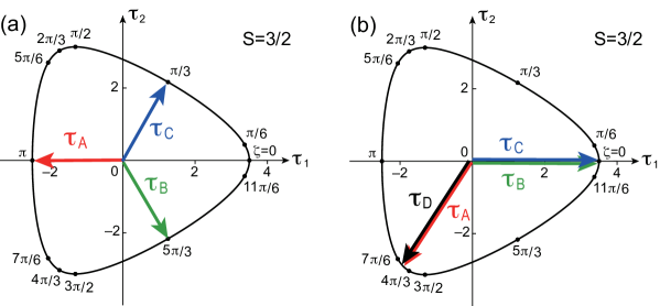
Figure 6: (a) The unique mean-field ground state for the triad of tetrahedron units $ABC$. (b) One of the mean-field ground states for the four units $ABCD$. This is also a solution in the bulk.

7.2 Solution for a triad of tetrahedron units

With this result, let us to find the lowest-energy solution for one tetrahedron triad, e.g. $ABC$. The corresponding mean field energy is

$$E_{\mathrm{MF}}(ABC)=-4J_{\mathrm{eff}}\Bigl{(}{\textstyle\frac{5}{4}}-\mathbf{e}_{0}\cdot\langle\bm{\tau}_{A}\rangle\Bigr{)}\Bigl{(}{\textstyle\frac{5}{4}}-\mathbf{e}_{1}\cdot\langle\bm{\tau}_{B}\rangle\Bigr{)}\Bigl{(}{\textstyle\frac{5}{4}}-\mathbf{e}_{2}\cdot\langle\bm{\tau}_{C}\rangle\Bigr{)},$$ (60)

and the mean field is, for example, $\mathbf{h}_{A}=-\mathbf{e}_{0}\bigl{(}{\textstyle\frac{5}{4}}-\mathbf{e}_{1}\cdot\langle\bm{\tau}_{B}\rangle\bigr{)}\bigl{(}{\textstyle\frac{5}{4}}-\mathbf{e}_{2}\cdot\langle\bm{\tau}_{C}\rangle\bigr{)}$. The lowest-energy solution is the one in which $\mathbf{e}(\theta_{X})\cdot\langle\bm{\tau}_{X}\rangle$=$-\frac{5}{2}$ for all the units $X$’s and its energy is $E_{\mathrm{MF}}(ABC)/(4J_{\mathrm{eff}})=-(15/4)^{3}\approx$$-52.73$. This means that the order parameters are $\langle\bm{\tau}(\zeta)\rangle$ with $\zeta$=$\pi$, $\frac{5}{3}\pi$, and $\frac{1}{3}\pi$ for $\theta_{X}$=0, $\frac{2}{3}\pi$, and $\frac{4}{3}\pi$. Thus, the mean field points towards the direction opposite to $\mathbf{e}(\theta_{X})$ at all the units, and the three $\langle\bm{\tau}\rangle$’s form an equilateral triangle. See Fig. 6(a). This solution has interesting spin correlations. In each tetrahedron unit, only one pair of bonds have a strong antiferromagnetic correlation

$$\langle\mathbf{S}_{1}\cdot\mathbf{S}_{2}\rangle_{A}=\langle\mathbf{S}_{3}\cdot\mathbf{S}_{4}\rangle_{A}=\langle\mathbf{S}_{1}\cdot\mathbf{S}_{3}\rangle_{B}=\langle\mathbf{S}_{2}\cdot\mathbf{S}_{4}\rangle_{B}=\langle\mathbf{S}_{1}\cdot\mathbf{S}_{4}\rangle_{C}=\langle\mathbf{S}_{2}\cdot\mathbf{S}_{3}\rangle_{C}=-{\textstyle\frac{15}{4}},$$ (61)

and $\langle\mathbf{S}_{i}\cdot\mathbf{S}_{j}\rangle_{X}=0$ for the other bonds. It is important to notice that these strong bonds are parts of the hexagon loop that connects the three tetrahedron units in $J^{\prime}$ perturbation. The strong bonds form a Kekulé pattern of antiferromagnetic correlation on the hexagon loop. The same behavior was already discovered in the $S=\frac{1}{2}$ case, and this is the origin of stability of the state obtained  Tsunetsugu1 ; Tsunetsugu2 ; Moessner .

7.3 Solution in the bulk

Let us examine the stability of this configuration when the fourth unit $D$ is attached. This also gives a solution in the bulk. Since the effective interaction takes effect for each triad of tetrahedron units, this attachment increases the number of interacting triads from 1 to 4. For the solution obtained in Sec. 7.2, I have found that all the new interactions relating to $D$ vanish as will be shown below. The mean field at the new unit $D$ is

$$\mathbf{h}_{D}=-\mathbf{e}_{0}\bigl{(}{\textstyle\frac{5}{4}}-\mathbf{e}_{1}\!\cdot\!\langle\bm{\tau}_{C}\rangle\bigr{)}\bigl{(}{\textstyle\frac{5}{4}}-\mathbf{e}_{2}\!\cdot\!\langle\bm{\tau}_{B}\rangle\bigr{)}-\mathbf{e}_{1}\bigl{(}{\textstyle\frac{5}{4}}-\mathbf{e}_{2}\!\cdot\!\langle\bm{\tau}_{A}\rangle\bigr{)}\bigl{(}{\textstyle\frac{5}{4}}-\mathbf{e}_{0}\!\cdot\!\langle\bm{\tau}_{C}\rangle\bigr{)}$$

$$\hskip 31.2982pt-\mathbf{e}_{2}\bigl{(}{\textstyle\frac{5}{4}}-\mathbf{e}_{0}\!\cdot\!\langle\bm{\tau}_{B}\rangle\bigr{)}\bigl{(}{\textstyle\frac{5}{4}}-\mathbf{e}_{1}\!\cdot\!\langle\bm{\tau}_{A}\rangle\bigr{)},$$ (62)

and this vanish if $\langle\bm{\tau}\rangle_{X}$ ($X=A,B,C$) are fixed as before, because each $(\frac{5}{4}-\mathbf{e}_{m}\cdot\langle\bm{\tau}_{X}\rangle)$ is zero in the equation above. Therefore, $\langle\bm{\tau}_{D}\rangle$ is undetermined and may point to any direction with no energy cost. This does not affect the mean fields $\mathbf{h}_{A-C}$, as far as $\langle\bm{\tau}_{A-C}\rangle$ are fixed to the values of the three-unit solution. For example, in Eq. (44) for $\mathbf{h}_{A}$, the parts $\mathbf{e}_{0}\cdot\langle\bm{\tau}_{B}\rangle$= $\mathbf{e}_{0}\cdot\langle\bm{\tau}_{C}\rangle$=$-\frac{1}{2}\langle\tau_{1,A}\rangle=\frac{5}{4}$ remove the contribution of $\langle\bm{\tau}_{D}\rangle$. Therefore, this is a self-consistent solution of the four-unit problem, and its total energy of the four units is identical to that of the three-unit solution. Thus the energy per triad increases. This situation happens in the $S=\frac{1}{2}$ case and its mean-field ground state in the four units $ABCD$ is continuously degenerate such that the direction of one $\langle\bm{\tau}\rangle$ is arbitrary  Tsunetsugu1 ; Tsunetsugu2 .

The situation completely changes in the $S$=$\frac{3}{2}$ case. The solution above is one self-consistent solution, but there exists another solution with a lower energy. This difference comes from the 3-fold anisotropy in the $\bm{\tau}$ space in the $S=\frac{3}{2}$ case, i.e., dependence of the ground state energy on the field direction $\epsilon_{0}(\zeta)$. I have numerically solved the mean-field equations for the 4 two-dimensional vectors $\{\langle\bm{\tau}_{X}\rangle\}$ ($X=A,B,C,D$), and found that the ground state is unique except 12-fold degeneracy due to the $T_{d}$ symmetry. All the 12 solutions have paired order parameters. One solution has the following ground state at each unit

$$\psi_{0}(A)=\psi_{0}(D) =\sqrt{0.2902}\,\Phi_{A_{1}}+\sqrt{0.0064}\,\Phi_{A_{2}}$$

$$\phantom{=}+\sqrt{0.7034}\,\bigl{(}\cos\xi_{AD}\,\Phi_{E_{u}}+\sin\xi_{AD}\,\Phi_{E_{v}}\bigr{)},\ \ \ (\xi_{AD}=-0.3473\pi)$$ (63a)

$$\psi_{0}(B)=\psi_{0}(C) =-{\textstyle\sqrt{\frac{3}{10}}}\,\Phi_{A_{1}}+{\textstyle\sqrt{\frac{7}{10}}}\,\Phi_{E_{u}}.$$ (63b)

Its order parameters pair up as

$$\langle\bm{\tau}_{A}\rangle=\langle\bm{\tau}_{D}\rangle\approx(-1.8969,-2.9187)=\langle\bm{\tau}(1.253\pi)\rangle,\ \ \langle\bm{\tau}_{B}\rangle=\langle\bm{\tau}_{C}\rangle=({\textstyle\frac{7}{2}},0)=\langle\bm{\tau}(0)\rangle.$$ (64)

and this corresponds to spin correlations

$$\begin{array}[]{cccc}\mbox{units}&\ \langle\mathbf{S}_{1}\cdot\mathbf{S}_{2}\rangle&\ \langle\mathbf{S}_{1}\cdot\mathbf{S}_{3}\rangle&\ \langle\mathbf{S}_{1}\cdot\mathbf{S}_{4}\rangle\\ \hline\cr\mbox{$A$ and $D$}&-3.1469&-2.8293&2.2261\\[2.0pt] \mbox{$B$ and $C$}&{\textstyle\frac{9}{4}}&-3&-3\end{array}$$ (65)

With these values, all the 4 three-body couplings in Eq. (41) for different triads have a negative value and thus lower the energy from the value for a tetrahedron triad, $E_{\mathrm{MF}}/(4J_{\mathrm{eff}})\approx-84.986<-52.73$. See also Table 1. This energy is the value for an isolated cluster of 4 tetrahedron units. I emphasize again that this is also a mean-field ground state in the bulk, and the bulk energy per cubic unit cell is four times of this value. Therefore the energy per spin is $E_{\mathrm{MF}}(\mbox{per spin})/(4J_{\mathrm{eff}})=-84.986\times\frac{4}{16}=-21.25$. This value does not contain the part of constant energy shift of orders $J^{\prime 2}/J$ and $J^{\prime 3}/J^{2}$.

Let me explain the degeneracy of this mean-field ground state. In the solution above, two $\langle\bm{\tau}\rangle$’s point along one of the trigonal axes $\mathbf{e}_{0}$. The other two $\langle\bm{\tau}\rangle$’s are slightly tilted from another trigonal axis $\mathbf{e}_{2}$, but that tilt is small (about $\frac{1}{60}\pi$). This solution is degenerate in two ways. First, it is degenerate with respect to change $\tau_{2}\rightarrow-\tau_{2}$. Secondly, the choice of two tetrahedron units are also arbitrary. One should note however that the trigonal axis to which their $\langle\bm{\tau}\rangle$’s point depends on which units are chosen. For example, in the case shown above, the units $B$ and $C$ have $\langle\bm{\tau}\rangle$ pointing to $\mathbf{e}_{0}$, which is related to 1-2 and 3-4 site pairs as shown in Eq. (42). This corresponds to the lattice structure, in which the $B$ unit is positioned from the nearest $C$ unit along the direction of either 1-2 or 3-4 bond. Since there are 6 ways of choosing two from $ABCD$, the total degeneracy of the mean-field ground state is $2\times 6$=12, and these solutions are related to each other by symmetry operations of the $T_{d}$ point group.

Table 1: Spin correlations between neighboring tetrahedron units in one mean-field ground state for the $S=\frac{3}{2}$ case. Each triple product corresponds to one term in $E_{\mathrm{MF}}$, and the four products are all negative. $X_{0}$ in the triple product $\pi(X_{0})$=$\langle\mathbf{S}_{1}\cdot\mathbf{S}_{2}\rangle_{X}$$\langle\mathbf{S}_{1}\cdot\mathbf{S}_{3}\rangle_{X^{\prime}}$$\langle\mathbf{S}_{1}\cdot\mathbf{S}_{4}\rangle_{X^{\prime\prime}}$ denotes the label of missing sublattice $X_{0}=\{A,B,C,D\}-\{X,X^{\prime},X^{\prime\prime}\}$.

$X$	$X^{\prime}$	$X^{\prime\prime}$	$\langle\mathbf{S}_{1}\cdot\mathbf{S}_{2}\rangle_{X}\!$	$\langle\mathbf{S}_{1}\cdot\mathbf{S}_{3}\rangle_{X^{\prime}}\!$	$\langle\mathbf{S}_{1}\cdot\mathbf{S}_{4}\rangle_{X^{\prime\prime}}\!$	triple product
A	B	C	$-3.1469$	$-3.0000$	$-3.0000$	$\pi(D)$=$-28.322$
B	A	D	$\phantom{-}2.2500$	$-2.8293$	$\phantom{-}2.2261$	$\pi(C)$=$-14.171$
C	D	A	$\phantom{-}2.2500$	$-2.8293$	$\phantom{-}2.2261$	$\pi(B)$=$-14.171$
D	C	B	$-3.1469$	$-3.0000$	$-3.0000$	$\pi(A)$=$-28.322$

8 Spin correlation in the mean-field ground state in the $S=\frac{3}{2}$ case

I now use two-spin correlations $\langle\mathbf{S}_{i}\cdot\mathbf{S}_{j}\rangle$ and reexamine symmetry breaking in the mean-field ground state obtained in the previous section. There are two types of these correlations: one type is the correlations on short bonds inside tetrahedron unit and the other is those on long bonds between neighboring units. As will be shown below, spin correlations are finite only between nearest-neighbor sites within the perturbative approach used in the present work. However, they manifest spontaneous breaking of the point group symmetry in spin-singlet order.

Spin correlations inside tetrahedron unit are already obtained during the calculation of the mean-field ground state, and their values are listed in Eq. (65). Recall that it is sufficient to see $f^{(1j)}=\langle\mathbf{S}_{1}\cdot\mathbf{S}_{j}\rangle$ ($j$=2, 3, and 4) because of the conjugate-pair equivalence. In the mean-field ground state for the $S=\frac{3}{2}$ case, two pairs have antiferromagnetic correlations and the other one is ferromagnetic in all the units. In two units among the four ($B$ and $C$ in Eq. (65)), the two antiferromagnetic correlations have the identical value $-3$, while they differ in the other two units.

8.1 Spin correlations between neighboring tetrahedron units for general $S$

Correlations between different units require a more elaborate calculation. This is because original spin degrees of freedom $\{\mathbf{S}_{j}(\mathbf{r})\}$ are traced out and the effective Hamiltonian has only spin-pair operators $\{\bm{\tau}(\mathbf{r})\}$ in each unit. In the effective Hamiltonian approach, correlations of traced-out degrees of freedom are to be calculated from the hybridization of ground-state wave function with excited states, and this generally needs additional careful perturbative calculation. For example, for the large-$U$ limit of the half-filled Hubbard model, Bulaevskii et al. derived an expression of charge density and current in terms of spin operators hubbard . In the present case, we can circumvent complicated calculation and obtain result quickly. The technique to use is Hellmann-Feynman theorem Hellmann . Let us temporarily generalize the original Hamiltonian such that weak couplings on long bonds are all different depending their positions, $J^{\prime}\rightarrow J_{ij}^{\prime}(\mathbf{r},\mathbf{r}^{\prime})$, and then its ground state energy is a function of these parameters, $E_{\mathrm{gs}}[\{J^{\prime}_{ij}(\mathbf{r},\mathbf{r}^{\prime})\}]$. Its derivative with respect to one parameter is the corresponding spin correlation, and we finally set all the parameters to a uniform value $J^{\prime}$ to come back to the original homogeneous Hamiltonian

$$\langle\mathbf{S}_{j_{1}}(\mathbf{r}_{1})\cdot\mathbf{S}_{j_{2}}(\mathbf{r}_{2})\rangle=\left.\frac{\partial E_{\mathrm{gs}}\bigl{[}\{J^{\prime}_{ij}(\mathbf{r},\mathbf{r}^{\prime})\}\bigr{]}}{\partial J^{\prime}_{j_{1},j_{2}}(\mathbf{r}_{1},\mathbf{r}_{2})}\right|_{\mathrm{all}\ J^{\prime}_{ij}(\mathbf{r},\mathbf{r}^{\prime})=J^{\prime}}.$$ (66)

The approximation in the present work replaces the ground state energy $E_{\mathrm{gs}}[\cdots]$ by $\varDelta E_{0}^{(2)}[\cdots]+\varDelta E_{0}^{(3)}[\cdots]+E_{\mathrm{MF}}[\cdots]$. Here, the last term is the mean-field ground state energy of $H_{\mathrm{eff}}$ and the first two terms are the energy shift in the second- and third-order perturbation

$$\varDelta E_{0}^{(2)}\bigl{[}\bigl{\{}J^{\prime}_{ij}(\mathbf{r},\mathbf{r}^{\prime})\bigr{\}}\bigr{]}=-\frac{\,3c_{0}^{2}\,}{2J}\sum_{\langle\mathbf{r},\mathbf{r}^{\prime}\rangle}J^{\prime}_{ij}(\mathbf{r},\mathbf{r}^{\prime})^{2},$$ (67a)

$$\varDelta E_{0}^{(3)}\bigl{[}\bigl{\{}J^{\prime}_{ij}(\mathbf{r},\mathbf{r}^{\prime})\bigr{\}}\bigr{]}=\phantom{-}\frac{\,9c_{0}^{3}\,}{2J^{2}}\!\sum_{\langle\mathbf{r}_{1},\mathbf{r}_{2},\mathbf{r}_{3}\rangle}J^{\prime}_{i,j}(\mathbf{r}_{1},\mathbf{r}_{2})J^{\prime}_{j,k}(\mathbf{r}_{2},\mathbf{r}_{3})J^{\prime}_{k,i}(\mathbf{r}_{3},\mathbf{r}_{1}).$$ (67b)

Recall that the combination of neighboring units, $\langle\mathbf{r},\mathbf{r}^{\prime}\rangle$ or $\langle\mathbf{r}_{1},\mathbf{r}_{2},\mathbf{r}_{3}\rangle$, automatically fixes the positions of connected sites, $ij$ or $ijk$. These energy shifts contribute a homogeneous part of spin correlations on long bonds

$$C_{\mathrm{inter}}\equiv\left.\frac{\partial(\varDelta E_{\mathrm{0}}^{(2)}+\varDelta E_{\mathrm{0}}^{(3)})\bigl{[}\bigl{\{}J^{\prime}_{ij}(\mathbf{r},\mathbf{r}^{\prime})\bigr{\}}\bigr{]}}{\partial J^{\prime}_{j_{1},j_{2}}(\mathbf{r}_{1},\mathbf{r}_{2})}\right|_{\mathrm{all}\ J^{\prime}_{ij}(\mathbf{r},\mathbf{r}^{\prime})=J^{\prime}}\!\!=-3c_{0}^{2}\,\rho+9c_{0}^{3}\,\rho^{2},$$ (68)

where $\rho\equiv J^{\prime}/J$ and the fact that each long bond is a part of two triangular loops is used for the part of $\varDelta E_{0}^{(3)}$.

Non-uniform correlations come from the mean-field energy $E_{\mathrm{MF}}[\cdots]$. Since we need a result only for its first order derivative, one can use for $E_{\mathrm{MF}}[\cdots]$ the value given from Eq. (41) by replacing $J_{\mathrm{eff}}$ with those local values calculated from $J_{ij}^{\prime}(\mathbf{r},\mathbf{r}^{\prime})$’s

$$E_{\mathrm{MF}}[\{J^{\prime}_{ij}(\mathbf{r},\mathbf{r}^{\prime})\}] =\frac{1}{6J^{2}}\sum_{\langle\mathbf{r}_{1},\mathbf{r}_{2},\mathbf{r}_{3}\rangle}J^{\prime}_{i_{1},j_{1}}(\mathbf{r}_{1},\mathbf{r}_{2})J^{\prime}_{j_{2},k_{1}}(\mathbf{r}_{2},\mathbf{r}_{3})J^{\prime}_{k_{2},i_{2}}(\mathbf{r}_{3},\mathbf{r}_{1})$$

$$\hskip 28.45274pt\times\bigl{(}-c_{0}+\mathbf{e}_{0}\cdot\langle\bm{\tau}_{\mathbf{r}_{1}}\rangle\bigr{)}\bigl{(}-c_{0}+\mathbf{e}_{1}\cdot\langle\bm{\tau}_{\mathbf{r}_{2}}\rangle\bigr{)}\bigl{(}-c_{0}+\mathbf{e}_{2}\cdot\langle\bm{\tau}_{\mathbf{r}_{3}}\rangle\bigr{)}.$$ (69)

This replacement is exact up to the first order in each coupling in $\{J_{ij}^{\prime}(\mathbf{r},\mathbf{r}^{\prime})\}$. The positions of connected sites, $i_{1},\cdots,i_{2}$, are also uniquely determined by the choice of three units $\langle\mathbf{r}_{1},\mathbf{r}_{2},\mathbf{r}_{3}\rangle$. Note that each weak coupling $J^{\prime}_{ij}(\mathbf{r},\mathbf{r}^{\prime})$ appears just in two terms in the sum above. It is helpful to notice that one does not need to consider the contribution of order parameter deformation $\partial\langle\bm{\tau}_{\mathbf{r}}\rangle/\partial J^{\prime}_{ij}(\mathbf{r}_{1},\mathbf{r}_{2})$ in Eq. (66). This is because the deformation couples to $\delta E_{\mathrm{MF}}/\delta\langle\bm{\tau}_{\mathbf{r}}\rangle$, and this vanishes since the mean-field solution minimizes $E_{\mathrm{MF}}$.

In the present case, all the bonds connecting the same pair of units $XX^{\prime}$ have an identical value of spin correlations. For example, in Fig. 4(a), $A1$ unit is connected to surrounding four $D$ units, and spin correlations are all the same: $\langle\mathbf{S}_{2}(A1)\cdot\mathbf{S}_{1}(D1)\rangle$= $\langle\mathbf{S}_{4}(A1)\cdot\mathbf{S}_{3}(D2)\rangle$= $\langle\mathbf{S}_{3}(A1)\cdot\mathbf{S}_{4}(D4)\rangle$= $\langle\mathbf{S}_{1}(A1)\cdot\mathbf{S}_{2}(D5)\rangle$. This value is given by summing the contributions of constant energy shift and the mean field energy

$$\langle\mathbf{S}_{i}(A)\cdot\mathbf{S}_{j}(D)\rangle =C_{\mathrm{inter}}+{\textstyle\frac{1}{6}}\rho^{2}\left[\bigl{(}-c_{0}+\mathbf{e}_{0}\cdot\langle\bm{\tau}_{C}\rangle\bigr{)}\bigl{(}-c_{0}+\mathbf{e}_{1}\cdot\langle\bm{\tau}_{D}\rangle\bigr{)}\bigl{(}-c_{0}+\mathbf{e}_{2}\cdot\langle\bm{\tau}_{A}\rangle\bigr{)}\right.$$

$$\hskip 62.59596pt\left.+\bigl{(}-c_{0}+\mathbf{e}_{0}\cdot\langle\bm{\tau}_{B}\rangle\bigr{)}\bigl{(}-c_{0}+\mathbf{e}_{1}\cdot\langle\bm{\tau}_{A}\rangle\bigr{)}\bigl{(}-c_{0}+\mathbf{e}_{2}\cdot\langle\bm{\tau}_{D}\rangle\bigr{)}\right]$$ (70a)

$$=C_{\mathrm{inter}}+{\textstyle\frac{1}{6}}\rho^{2}\bigl{[}\pi(B)+\pi(C)\bigr{]},$$ (70b)

where $\pi(X)$’s are triple products defined in Table 1. The part of $E_{\mathrm{MF}}$ contributes two terms $\pi(B)$ and $\pi(C)$ corresponding to 2 hexagon loops shown in Fig. 2.

For correlations of other pairs of sublattices, similar results are obtained and the combinations of the three units on the right-hand side are easily read from Eq. (41)

$$I_{X_{1}X_{2}}\equiv\langle\mathbf{S}_{i}(X_{1})\cdot\mathbf{S}_{j}(X_{2})\rangle=C_{\mathrm{inter}}+{\textstyle\frac{1}{6}}\rho^{2}\bigl{[}\pi(Y_{1})+\pi(Y_{2})\bigr{]},\ \ \ (X_{1}\neq X_{2})$$ (71)

where $Y$’s are determined by the complementary condition $\{Y_{1},Y_{2}\}=\{A,B,C,D\}-\{X_{1},X_{2}\}$. For example, $I_{AC}$ is related to $\pi(B)+\pi(D)$. This leads to an important identity for the spin correlations between neighboring units, and this is a relation about correlations on different pairs of long bonds

$$I_{AB}+I_{CD}=I_{AC}+I_{BD}=I_{AD}+I_{BC}=2C_{\mathrm{inter}}+{\textstyle\frac{1}{6}}\rho^{2}\sum_{X=A}^{D}\pi(X)=:2\bar{I}_{\mathrm{inter}}.$$ (72)

One should note that this identity holds generally for any mean-field solution. In the solution obtained in the previous section for the $S=\frac{3}{2}$ case, the order parameters pair up as $\langle\bm{\tau}_{A}\rangle$=$\langle\bm{\tau}_{D}\rangle$ and $\langle\bm{\tau}_{B}\rangle$=$\langle\bm{\tau}_{C}\rangle$, which leads to $\langle\pi(A)\rangle$=$\langle\pi(D)\rangle$ and $\langle\pi(B)\rangle$=$\langle\pi(C)\rangle$, but this degeneracy is not necessary for the above identity.

Like the case of the effective Hamiltonian, the results for the spin correlations obtained up to this stage hold for general $S$.

Figure 7: Two-spin correlations in the $S=\frac{3}{2}$ Heisenberg model on the breathing pyrochlore lattice. In each tetrahedron unit, antiferromagnetic correlations are shown by straight lines and their line width schematically shows $|\mathbf{S}_{i}\cdot\mathbf{S}_{j}|$, while zigzag lines show ferromagnetic correlations. Dashed lines show weak antiferromagnetic correlations between neighboring units, and they are of order $(J^{\prime}/J)^{1}$ at most.

8.2 Results of the $S=\frac{3}{2}$ case

I now apply the derived formula to the $S=\frac{3}{2}$ case and calculate spin correlations on long bonds connecting neighboring tetrahedron units. For this case, the constant value is $C_{\mathrm{inter}}=-\frac{75}{16}\rho+\frac{1125}{64}\rho^{2}\approx-4.6875\rho+17.578\rho^{2}$. Triple products $\pi(X)$’s are already calculated and listed in Table 1. Using these results up to $\rho^{2}$, the spin correlations on the long bonds are given as

$$\left\{\begin{array}[]{lll}\displaystyle I_{XY}=\langle\mathbf{S}_{i}(X)\cdot\mathbf{S}_{j}(Y)\rangle&=-{\textstyle\frac{75}{16}}\rho+10.4959\rho^{2}&=:I_{0},\hskip 14.22636pt\bigl{(}X\in\{A,D\},\ Y\in\{B,C\}\bigr{)}\\[5.0pt] \displaystyle I_{AD}=\langle\mathbf{S}_{i}(A)\cdot\mathbf{S}_{j}(D)\rangle&=-{\textstyle\frac{75}{16}}\rho+12.8544\rho^{2}&=:I_{1},\\[5.0pt] \displaystyle I_{BC}=\langle\mathbf{S}_{i}(B)\cdot\mathbf{S}_{j}(C)\rangle&=-{\textstyle\frac{75}{16}}\rho+\phantom{1}8.1371\rho^{2}&=:I_{2}.\end{array}\right.$$ (73)

This result shows that all the long bonds between tetrahedron units have an antiferromagnetic correlation, at least if the exchange coupling on long bonds is small enough $\rho\ll 1$. This is natural since the exchange coupling $J^{\prime}$ on long bonds is antiferromagnetic. The $\rho^{2}$ terms contribute ferromagnetic correlations, and this comes from the constant energy shift $\varDelta E_{0}^{(3)}$. As $\pi(X)<0$ for all $X$’s, $E_{\mathrm{MF}}$ yields antiferromagnetic contribution and this part is the origin of the difference between the three $I$’s. This result (73) is for one of the degenerate mean-field ground states, and spin correlations in other states are obtained by a symmetry operation in the $T_{d}$ point group.

Figure 7 illustrates spin correlations on short bonds in tetrahedron units as well as those on long bonds connecting neighboring units. The original tetrahedral symmetry $T_{d}$ of the units are lowered to $D_{2d}$ in the two units with higher symmetry and $D_{2}$ in the other two units. Note that $D_{2}$ is the lowest possible symmetry, since the equivalence relations should hold, and this is the point group symmetry of the entire system.

8.3 Spin structure factor for the $S=\frac{3}{2}$ case

Finally, I analyze spin structure factor. For that, I use the following definition

$$S_{\mu\nu}(\mathbf{q})\equiv\frac{1}{N}\sum_{\mathbf{r},i}\sum_{\mathbf{r}^{\prime},j}\langle{S}_{i}^{\mu}(\mathbf{r}){S}_{j}^{\nu}(\mathbf{r}^{\prime})\rangle e^{-i\mathbf{q}\cdot(\mathbf{r}+\bm{\delta}_{i}-\mathbf{r}^{\prime}-\bm{\delta}_{j})}={\textstyle\frac{1}{3}}\delta_{\mu\nu}S(\mathbf{q}),$$ (74)

where $\bm{\delta}_{i}$ and $\bm{\delta}_{j}$ are the position of the $i$-th and $j$-th spin in tetrahedron unit. Instead of considering structure factor for each $ij$-pair, I alternatively define this for $\mathbf{q}$ in the extended Brillouin zone, not limited to the reduced zone. $S(\mathbf{q})$ has no Bragg peaks and is isotropic in the spin space, because of the absence of magnetic dipole order, and this is a smooth function of $\mathbf{q}$. Naturally, one divides $S(\mathbf{q})$ into two parts which correspond to correlations inside tetrahedron units and those between units:

$$S(\mathbf{q})=S_{\mathrm{intra}}(\mathbf{q})+S_{\mathrm{inter}}(\mathbf{q}).$$ (75)

The first part is calculated from spin correlations on short bonds, and the result is given by

$$S_{\mathrm{intra}}(\mathbf{q})={\textstyle\frac{15}{4}}+\bar{f}^{(12)}\gamma_{xy}(\mathbf{q}\,a_{S})+\bar{f}^{(13)}\gamma_{zx}(\mathbf{q}\,a_{S})+\bar{f}^{(14)}\gamma_{yz}(\mathbf{q}\,a_{S}),$$ (76)

where the constant term is $S(S+1)$. Here, the form factor is $\gamma_{\mu\nu}(\bar{\mathbf{q}})=\cos(2\bar{q}_{\mu})\cos(2\bar{q}_{\nu})$ with $\sqrt{2}a_{s}$ being the length of short bonds in tetrahedron units. $\bar{f}^{(ij)}=\frac{1}{4}\sum_{X=A}^{D}\langle\mathbf{S}_{i}\cdot\mathbf{S}_{j}\rangle_{X}$ is the average spin correlation between the spin pair $i$ and $j$ inside tetrahedron unit, and this is anisotropic in space depending on the bond direction;

$$\bar{f}^{(12)}=-0.4485,\ \bar{f}^{(13)}=-2.9147,\ \bar{f}^{(14)}=-0.3870,$$ (77)

and I have used the conjugate-pair equivalence, $\bar{f}_{12}=\bar{f}_{34}$ etc. To see the spatial anisotropy in more detail, I rewrite the $\mathbf{q}$-dependence and separate the part with cubic symmetry

$$S_{\mathrm{intra}}(\mathbf{q})={\textstyle\frac{15}{4}}+\bar{f}_{\mathrm{cub}}\,\gamma_{\mathrm{cub}}(\mathbf{q}\,a_{S})+\bar{f}_{u}\gamma_{u}(\mathbf{q}\,a_{S})+\bar{f}_{v}\gamma_{v}(\mathbf{q}\,a_{S}),$$ (78)

where

$$\gamma_{\mathrm{cub}}=\gamma_{xy}+\gamma_{yz}+\gamma_{zx},\ \gamma_{u}={\textstyle\frac{1}{\sqrt{6}}}(2\gamma_{xy}-\gamma_{yz}-\gamma_{zx}),\ \gamma_{v}={\textstyle\frac{1}{\sqrt{2}}}(\gamma_{yz}-\gamma_{zx}),$$ (79)

and the amplitudes are given by

$$\bar{f}_{\mathrm{cub}}={\textstyle\frac{1}{3}}(\bar{f}^{(12)}+\bar{f}^{(14)}+\bar{f}^{(13)})=-{\textstyle\frac{1}{3}}S(S+1)=-{\textstyle\frac{5}{4}},$$

$$\bar{f}_{u}={\textstyle\frac{1}{\sqrt{6}}}(2\bar{f}^{(12)}-\bar{f}^{(14)}-\bar{f}^{(13)})=0.9817,\hskip 19.91684pt\bar{f}_{v}={\textstyle\frac{1}{\sqrt{2}}}(\bar{f}^{(14)}-\bar{f}^{(13)})=1.7874,$$ (80)

The cubic part of the $\mathbf{q}$-dependence is $\gamma_{\mathrm{cub}}$, and $\gamma_{u}$ and $\gamma_{v}$ represent spatially anisotropic components of spin correlations that transforms following $E$-irrep of the $T_{d}$ point group.

The contribution of correlations between neighboring tetrahedron units is generally given as

$$S_{\mathrm{inter}}(\mathbf{q})={\textstyle\frac{1}{4}}\Bigl{[}(I_{AB}+I_{CD})\gamma_{yz}(\mathbf{q}\,a_{L})+(I_{AC}+I_{BD})\gamma_{zx}(\mathbf{q}\,a_{L})+(I_{AD}+I_{BC})\gamma_{xy}(\mathbf{q}\,a_{L})\Bigr{]},$$ (81)

where $\sqrt{2}a_{L}$ is the length of long bonds connecting tetrahedron units. $I_{XY}$’s values are listed in Eq. (73). The identity (72) guarantees that the three $\gamma$’s have a common amplitude, and its value is $\frac{1}{2}\bar{I}_{\mathrm{inter}}=-\frac{75}{32}\rho+5.2480\rho^{2}$. Adding up the two parts, one obtains the final result of the spin structure factor

$$S(\mathbf{q})={\textstyle\frac{15}{4}} \Bigl{[}1-{\textstyle\frac{1}{3}}\gamma_{\mathrm{cub}}(\mathbf{q}\,a_{S})-\bigl{(}{\textstyle\frac{5}{8}}\rho-1.3995\rho^{2}\bigr{)}\gamma_{\mathrm{cub}}(\mathbf{q}\,a_{L})+0.2618\gamma_{u}(\mathbf{q}\,a_{S})+0.4766\gamma_{v}(\mathbf{q}\,a_{S})\Bigr{]},$$ (82)

where the constant part $S(S+1)=\frac{15}{4}$ is factored out and again $\rho=\frac{J^{\prime}}{J}$.

9 Mean field ground state of the effective model in the $S=1$ case

Now that we have found that the mean-field ground state in the breathing pyrochlore model differ between the two cases of $S=\frac{1}{2}$ and $\frac{3}{2}$, a natural question arises about the intermediate case of $S=1$. It turns out that the result is similar to the $S=\frac{3}{2}$ case, and I will sketch calculations.

In the case of $S=1$, the $S_{\mathrm{unit}}=0$ space at each tetrahedron unit has now dimension 3 and consists of basis states belonging to $A_{1}$- and $E$-irreps

$$\Phi_{A_{1}}={\textstyle\frac{1}{3}}\bigl{(}\sqrt{5}\Phi_{0}+2\Phi_{2}\bigr{)},\hskip 8.5359pt\Phi_{Eu}={\textstyle\frac{1}{3}}\bigl{(}2\Phi_{0}-\sqrt{5}\Phi_{2}\bigr{)},\hskip 8.5359pt\Phi_{Ev}=-\Phi_{1}.$$ (83)

The effective Hamiltonian is the one in Eq. (22) as before, but the constant is $c_{0}=\frac{2}{3}$ and the two operators are now represented as follows with the local basis set $\{\Phi_{A_{1}},\Phi_{Eu},\Phi_{Ev}\}$,

$$\tau_{1}=\frac{1}{3}\left[\begin{array}[]{ccc}0&-2\sqrt{5}&0\\ -2\sqrt{5}&1&0\\ 0&0&-1\end{array}\right],\ \ \tau_{2}=\frac{1}{2}\left[\begin{array}[]{ccc}0&0&2\sqrt{5}\\ 0&0&1\\ 2\sqrt{5}&1&0\end{array}\right].\ \$$ (84)

Figure 8: One mean-field ground state of the effective Hamiltonian for $S=1$. Trajectory is the ground state value of $\langle\bm{\tau}(\zeta)\rangle$, and the expectation value $\langle\psi|\bm{\tau}|\psi\rangle$ calculated for any state $\psi$ should be located on or inside this trajectory. Two bounds are $\langle\tau_{1}(\zeta=0)\rangle=\frac{5}{3}$ and $\langle\tau_{1}(\pi)\rangle=-\frac{4}{3}$.

I have used the mean field approximation again for the $S=1$ case, and it goes exactly the same as before. A necessary calculation is a solution of the eigenvalue problem for a $3\times 3$ matrix of the local mean field Hamiltonian (43). I have diagonalized the reduced Hamiltonian $\bar{H}_{\mathrm{MF}}(\zeta)$, and found that its lowest eigenvalue is given as

$$\epsilon_{0}(\zeta)=-\frac{2\sqrt{7}}{3}\cos\left[\frac{1}{3}\cos^{-1}\left(\frac{10}{7^{3/2}}\cos 3\zeta\right)\right].$$ (85)

At the tetrahedron unit where the mean field $\mathbf{h}$ points to the direction $\mathbf{e}(\mathbf{\zeta})$, the order parameter is given by Eq. (54) with this new result. Its trajectory upon varying $\zeta$ from 0 to $2\pi$ is plotted in Fig. 8, and this has a shape of rounded triangle as in the $S=\frac{3}{2}$ case. This manifests anisotropy in the order parameter space, but the anisotropy is smaller compared to the $S=\frac{3}{2}$ case. As shown in Eq. (49), the anisotropy defined in the order parameter space is $R_{\mathrm{anis}}=\frac{5}{4}$, which is smaller than $R_{\mathrm{anis}}=\frac{7}{5}$ for $S=\frac{3}{2}$.

The mean-field ground state for a tetrahedron triad does not depend on the $S$ value and the order parameters at the units $ABC$ have the same configuration as the one shown in Fig. 6(a). A mean-field ground state in the tetrahedron quartet $ABCD$ is also a solution in the bulk. Minimizing the mean field energy (40) with respect to the four order parameters $\langle\bm{\tau}\rangle$’s, I have searched ground states and found 12 solutions. One of them is

$$\langle\bm{\tau}_{A}\rangle=\langle\bm{\tau}_{D}\rangle\approx(-1.0064,-1.2917)=\langle\bm{\tau}(1.215\pi)\rangle,\ \ \langle\bm{\tau}_{B}\rangle=\langle\bm{\tau}_{C}\rangle=({\textstyle\frac{5}{3}},0)=\langle\bm{\tau}(0)\rangle.$$ (86)

These values are plotted in Fig. 8, and this solution has the same nature of the solution in the $S=\frac{3}{2}$ case in Fig. 6(b). The spin correlations are as follows

$$\begin{array}[]{cccc}\mbox{units}&\langle\mathbf{S}_{1}\cdot\mathbf{S}_{2}\rangle&\langle\mathbf{S}_{1}\cdot\mathbf{S}_{3}\rangle&\langle\mathbf{S}_{1}\cdot\mathbf{S}_{4}\rangle\\ \hline\cr\mbox{$A$ and $D$}&-1.6731&-1.2821&0.9552\\[2.0pt] \mbox{$B$ and $C$}&1&-{\textstyle\frac{3}{2}}&-{\textstyle\frac{3}{2}}\end{array}$$ (87)

Triple products in $E_{\mathrm{MF}}$ are all negative: $\pi(A)=\pi(D)=-3.7645$ and $\pi(B)=\pi(C)=-1.2247$. The relative difference between these two values is larger compared to the result for the $S=\frac{3}{2}$ case shown in Table  1. This is because $|\langle\bm{\tau}_{A,D}\rangle|$ is shorter than $|\langle\bm{\tau}_{B,C}\rangle|$ by about 1.8% here, while the reduction is only 0.5% in the $S=\frac{3}{2}$ case.

I have repeated the same calculation as in Sec. 8.3 and calculated spin structure factor for the $S=1$ case

$$S(\mathbf{q})=2 \Bigl{[}1-{\textstyle\frac{1}{3}}\gamma_{\mathrm{cub}}(\mathbf{q}\,a_{S})-\bigl{(}{\textstyle\frac{1}{3}}\rho-0.4588\rho^{2}\bigr{)}\gamma_{\mathrm{cub}}(\mathbf{q}\,a_{L})+0.2022\gamma_{u}(\mathbf{q}\,a_{S})+0.3955\gamma_{v}(\mathbf{q}\,a_{S})\Bigr{]},$$ (88)

where again $\rho=\frac{J^{\prime}}{J}$. Compared to the $S=\frac{3}{2}$ case, the structure factor has smaller amplitudes in its anisotropic parts $\gamma_{u}$ and $\gamma_{v}$. This is related to the fact that the anisotropy $R_{\mathrm{anis}}$ in the order parameter is smaller for $S=1$.

10 Summary

In this paper, I have studied the ground state of the antiferromagnetic spin-$S$ Heisenberg spin model on a breathing pyrochlore lattice, and examined a spontaneous breaking of lattice symmetry in the spin-singlet subspace. This lattice has two types of bonds, short and long, and the ratio of the corresponding exchange couplings $J^{\prime}/J$ controls frustration. In the limit of $J^{\prime}$=0, the ground state is thermodynamically degenerate and the main issue is what is the ground state when $0<J^{\prime}\ll J$ and what type of spatial pattern do spin correlations show in the symmetry broken ground state.

Based on the third-order perturbation in $J^{\prime}$, I have derived an effective Hamiltonian for general $S$, and examined spin-singlet orders with broken lattice symmetry. It is noticeable that the effective Hamiltonian has a form of three-tetrahedron interactions that is identical to the one of the $S$=$\frac{1}{2}$ case previously studied, and I have shown this with the help of newly found two identities of spin-pair operators. This Hamiltonian is represented in terms of two types of pseudospin operators $\bm{\tau}$, and they describe nonuniform correlations of four spins inside the unit. Despite of the identical form of the Hamiltonian, the dimension of $\bm{\tau}$’s local Hilbert space increases as $2S+1$ with spin. Since their matrix elements were not known, I have used algebras of four-spin composition and calculated these matrix elements for general $S$.

Using these results, I have analyzed the effective model by a mean-field approximation and investigated its ground state for the special cases of $S$=$\frac{3}{2}$ and 1. I have found that the response of pseudospins has a $Z_{3}$ anisotropy in $(\tau_{1},\tau_{2})$ space when $S>\frac{1}{2}$, and this has a critical effect on pseudospin orders. In contrast to the previous case of $S$=$\frac{1}{2}$, the ground state of four tetrahedron units has only a few stable configurations, and they have no further frustration when the configuration is repeated in space. Thus, this is the ground state of the entire system within the mean-field approximation. Actually, the ground state is uniquely determined in the sense that multiple solutions are related to each other by the lattice symmetry.

I have studied in detail spatial pattern of spin correlations in the ground state. Each tetrahedron unit exhibits one of the two types of internal spin correlations as shown in Fig. 7. Among six bonds in each unit, four bonds have either strong or weak antiferromagnetic spin correlations, while the other two bonds have ferromagnetic correlations. As for correlations between different units, they are always antiferromagnetic. I have also calculated the spin structure factor $S(\mathbf{q})$, which may be compared to the energy-integrated value of neutron inelastic scattering. It is found that the amplitude of symmetry broken parts $\bar{f}_{u}$, $\bar{f}_{v}$ is comparable to the symmetric part $\bar{f}_{\mathrm{cub}}$.

Quantum fluctuations between different units are neglected in the present work, but two features may justify this approximation. One is the three-dimensionality of the lattice, and quantum fluctuations are much smaller than in lower-dimensional cases. The second reason is the presence of the $Z_{3}$ anisotropy. A half of the local order parameters point to one of the directions that minimize the anisotropy energy, and the other half also only slightly tilt from another lowest-energy direction. Therefore, their fluctuations are expected not so large.

Finally, I make a comment on the implication of the present result for interpreting experiment results in the Li$X$Cr₄O₈ compounds. It is not fair to compare the theoretical results of this work to experimental work, since the present theory does not take account of two important features in these materials. One is the magnetoelastic effects, i.e., coupling of spins and phonons. This is particularly important because the ground state of the spin system breaks the lattice translation and rotation symmetries. Coupling to the corresponding phonon modes should have a large contribution to the ground state energy, and this may change relative stability among different quantum states. The other is the spin anisotropy due to large $S$-value. It is legitimate to assume that orbital angular moments of Cr ions are quenched as a starting point, but fluctuations in Cr valency are not zero and this leads to anisotropic corrections to the Heisenberg couplings. I believe that despite these points the results and predictions in the present work are useful for discussing magnetic parts of possible symmetry breaking in the breathing pyrochlore materials.

Appendix A Classification of tetrahedron singlet states

In this appendix, I classify the $(2S+1)$-fold singlet ground states in tetrahedron unit according to $T_{d}$ point group symmetry. This point group has one trivial and four other conjugacy classes of symmetry operations, and the nontrivial classes are represented by the following permutations of the four sites

$$\mbox{IC${}_{4}$: }(1423)=P_{2},\ \ \mbox{C${}_{2}$: }(12)(34)=P_{3},\ \ \mbox{$\sigma_{d}$: }(12)(3)(4)=P_{4},\ \ \mbox{C${}_{3}$: }(1)(234)=P_{5},$$ (89)

where each parenthesis denotes the cyclic permutation of its contained sites Messiah . For a permutation $P_{n}$ in each conjugacy class, its representation in terms of the singlet states is thus given by

$$\bigl{(}P_{n}\bigr{)}_{l^{\prime},l}=\langle\Phi_{l^{\prime}}|P_{n}|\Phi_{l}\rangle.$$ (90)

Since operating permutation $P$ changes the way of spin combination in the basis states (3), it is convenient to generalize the definition of basis states to

$$\Phi_{l}^{(ij)(mn)}=\sum_{l_{z}=-l}^{l}C(l,l_{z})\phi^{(ij)}(l,l_{z})\otimes\phi^{(mn)}(l,-l_{z}),$$ (91)

and the original ones are $\Phi_{l}=\Phi_{l}^{(12)(34)}$. The properties (5) and $C(l,-l_{z})=C(l,l_{z})$ lead to the following symmetry in the generalized basis states

$$\Phi_{l}^{(ij)(mn)}=(-1)^{2S+l}\Phi_{l}^{(ji)(mn)}=(-1)^{2S+l}\Phi_{l}^{(ij)(nm)}=\Phi_{l}^{(ji)(nm)},$$ (92)

$$\Phi_{l}^{(mn)(ij)}=\Phi_{l}^{(ij)(mn)}.$$ (93)

It is ready to calculate the representation matrix for $P_{3}$, $P_{4}$, and $P_{2}$. Operating these permutations, we obtain

$$P_{3}\Phi_{l}=\Phi_{l}^{(21)(43)}=\Phi_{l},\ \ P_{4}\Phi_{l}=\Phi_{l}^{(21)(34)}=(-1)^{2S+l}\Phi_{l},\ \ P_{2}\Phi_{l}=\Phi_{l}^{(43)(12)}=(-1)^{2S+l}\Phi_{l},$$ (94)

and therefore the representation matrix is $(P_{2})_{ll^{\prime}}=(P_{4})_{ll^{\prime}}=(-1)^{2S+l}\delta_{ll^{\prime}}$ and $(P_{3})_{ll^{\prime}}=\delta_{ll^{\prime}}$. The character of their corresponding conjugacy classes is the trace of the representation matrices, and the result is $\chi(IC_{4})=\chi(\sigma_{d})=\mbox{mod }(2S-1,2)$ and $\chi(C_{2})=2S+1$.

As for $P_{5}$, we need to directly calculate the matrix element

$$\bigl{(}P_{5}\bigr{)}_{l^{\prime}l}=\langle\Phi_{l^{\prime}}^{(12)(34)}|\Phi_{l}^{(13)(42)}\rangle=(-1)^{2S+l}\langle\Phi_{l^{\prime}}^{(12)(34)}|\Phi_{l}^{(13)(24)}\rangle.$$ (95)

This overlap of the two wavefunctions is a complicated factor that is related to the combination of four spins in two ways. Therefore it is possible to represent this with the Wigner’s $9j$-symbol Messiah

$$\langle\Phi_{l^{\prime}}^{(12)(34)}|\Phi_{l}^{(13)(24)}\rangle=(2l+1)(2l^{\prime}+1)\left\{\begin{array}[]{ccc}S&S&l^{\prime}\\ S&S&l^{\prime}\\ l&l&0\end{array}\right\}.$$ (96)

This can be further simplified by using a reduction formula of the $9j$-symbol to a $6j$-symbol Messiah , and we obtain

$$\bigl{(}P_{5}\bigr{)}_{l^{\prime}l}=\langle\Phi_{l^{\prime}}^{(12)(34)}|P_{5}|\Phi_{l}^{(12)(34)}\rangle=(-1)^{l^{\prime}}\sqrt{(2l+1)(2l^{\prime}+1)}\left\{\begin{array}[]{ccc}S&S&l^{\prime}\\ S&S&l\end{array}\right\}.$$ (97)

Finally, the character of the $C_{3}$ conjugacy class is

$$\chi(C_{3})=\mbox{Tr }P_{5}=\sum_{l=0}^{2S}(-1)^{l}(2l+1)\left\{\begin{array}[]{ccc}S&S&l\\ S&S&l\end{array}\right\}=\mbox{mod }(2S-1,3)-1,$$ (98)

where the last expression is derived based on the numerical results up to $S=6$.

Table 2: Character table of the $T_{d}$ group. The last row is for the representation in terms of tetrahedron singlet states $\{\Phi_{l}\}$. See Ref. group for the irreps.

$T_{d}$	$E$	6$IC_{4}$	3$C_{2}$	6$\sigma_{d}$	8$C_{3}$
A1	1	$\phantom{-}1$	$\phantom{-}1$	$\phantom{-}1$	$\phantom{-}1$
A2	1	$-1$	$\phantom{-}1$	$-1$	$\phantom{-}1$
E${}_{\phantom{2}}$	2	$\phantom{-}0$	$\phantom{-}2$	0	$-1$
T1	3	$\phantom{-}1$	$-1$	$-1$	$\phantom{-}0$
T2	3	$-1$	$-1$	1	$\phantom{-}0$
$\Gamma_{\Phi}$	$2S+1$	$\mbox{mod }(2S-1,2)$	$2S+1$	$\mbox{mod }(2S-1,2)$	$\mbox{mod }(2S-1,3)-1$

Table 3: Multiplicity of the three irreps in $\Gamma_{\Phi}^{(S)}$ for $S\leq 4$. $\chi_{2}$=$\chi(IC_{4})$ and $\chi_{5}$=$\chi(C_{3})$. The multiplicity is 0 for the $T_{1}$- and $T_{2}$-irreps.

$S$	$\chi_{2}$	$\chi_{5}$	$n(\mathrm{A}_{1};S)$	$n(\mathrm{A}_{2};S)$	$n(\mathrm{E};S)$
$\textstyle\frac{1}{2}$	0	$-1$	0	0	1
1	1	$\phantom{-}0$	1	0	1
$\textstyle\frac{3}{2}$	0	$\phantom{-}1$	1	1	1
2	1	$-1$	1	0	2
$\textstyle\frac{5}{2}$	0	$\phantom{-}0$	1	1	2
3	1	$\phantom{-}1$	2	1	2
$\textstyle\frac{7}{2}$	0	$-1$	1	1	3
4	1	$\phantom{-}0$	2	1	3

The character of the conjugacy classes is listed in Table 2, and it is interesting that the result is periodic in $S$ with period 3 except for the $E$ and $C_{2}$ classes.

Using this character table, one can reduce the representation $\Gamma_{\Phi}^{(S)}$ by the tetrahedron singlet states $\{\Phi_{l}\}$ to the irreps group : $\Gamma_{\phi}^{(S)}=\sum_{\Gamma}n(\Gamma;S)\Gamma$ where $\Gamma$’s are the five irreps. The multiplicity is

$$n(\mathrm{A}_{1};S)=\frac{2S+1+3\chi_{2}+2\chi_{5}}{6},\ \ n(\mathrm{A}_{2};S)=\frac{2S+1-3\chi_{2}+2\chi_{5}}{6},\ \$$

$$n(\mathrm{E};S)=\frac{2S+1-\chi_{5}}{3},\ \ n(\mathrm{T}_{1};S)=n(\mathrm{T}_{2};S)=0,$$ (99)

where $\chi_{2}=\chi(IC_{4})=\mbox{mod }(2S-1,2)$ and $\chi_{5}=\chi(C_{3})=\mbox{mod }(2S-1,3)-1$. The results are shown for $S\leq 4$ in Table  3. The periodicity in $\chi_{2}$ and $\chi_{5}$ leads to the following recursion formula

$$n(\mathrm{A}_{1};S+3)=n(\mathrm{A}_{1};S)+1,\ \ n(\mathrm{A}_{2};S+3)=n(\mathrm{A}_{2};S)+1,\ \ n(\mathrm{E};S+3)=n(\mathrm{E};S)+2.$$ (100)

Appendix B Relation of $F_{l^{\prime}l}^{(12)}$, $F_{l^{\prime}l}^{(13)}$ and $F_{l^{\prime}l}^{(14)}$

In this appendix, I explain how to calculate matrix elements of $\mathbf{S}_{1}\cdot\mathbf{S}_{j}$ between two basis states $\Phi_{l}$’s in the $S_{\mathrm{unit}}=0$ subspace in a tetrahedron unit. These states are defined in Eq. (3) in terms of two spin-pair wavefunctions $\phi^{(12)}(l,l_{z})$ and $\phi^{(34)}(l,-l_{z})$. Introducing composite spin operators $\mathbf{S}_{ij}\equiv\mathbf{S}_{i}+\mathbf{S}_{j}$, this $\phi^{(12)}(l,l_{z})$ is an eigenstate of $\mathbf{S}_{12}^{2}$ with eigenvalue $l(l+1)$. Summing up for $l_{z}$, the same is true about $\Phi_{l}$ and

$$l(l+1)\Phi_{l}=\mathbf{S}_{12}^{2}\Phi_{l}=2\bigl{[}S(S+1)+\mathbf{S}_{1}\cdot\mathbf{S}_{2}\bigr{]}\Phi_{l}=2\bigl{[}S(S+1)+\mathbf{S}_{3}\cdot\mathbf{S}_{4}\bigr{]}\Phi_{l}.$$ (101)

Therefore, $\Phi_{l}$ is an eigenstate of $\mathbf{S}_{1}\cdot\mathbf{S}_{2}$ and its eigenvalue is $\frac{1}{2}l(l+1)-S(S+1)$ and therefore

$$F_{l^{\prime}l}^{(12)}\equiv\langle\Phi_{l^{\prime}}|{\textstyle\frac{1}{3}}S(S+1)+\mathbf{S}_{1}\cdot\mathbf{S}_{2}|\Phi_{l}\rangle=\bigl{[}{\textstyle\frac{1}{2}}l(l+1)-{\textstyle\frac{2}{3}}S(S+1)\bigr{]}\delta_{l^{\prime}l}.$$ (102)

This matrix is traceless, $\sum_{l=0}^{2S}F_{ll}^{(12)}=0$.

Matrix elements of $\mathbf{S}_{1}\cdot\mathbf{S}_{3}$ and $\mathbf{S}_{1}\cdot\mathbf{S}_{4}$ need more elaborate calculations, since the spin pair 1-3 or 1-4 does not match the construction of the basis states $\Phi_{l}$’s. It is useful to notice that these are related to each other through the cyclic permutation $P_{5}$ introduced in Eq. (89). The operation $P_{5}$ changes the sites 2, 3, and 4 to 3, 4, and 2, respectively, while $P_{5}^{-1}=P_{5}^{2}$ changes to 4, 2, and 3. Therefore, one obtains

$$\mathbf{S}_{1}\cdot\mathbf{S}_{3}=P_{5}\bigl{(}\mathbf{S}_{1}\cdot\mathbf{S}_{2}\bigr{)}P_{5}^{-1},\ \ \mathbf{S}_{1}\cdot\mathbf{S}_{4}=P_{5}^{-1}\bigl{(}\mathbf{S}_{1}\cdot\mathbf{S}_{2}\bigr{)}P_{5}.$$ (103)

This immediately leads to the relations between $F^{(1j)}$’s:

$$\mathsf{F}^{(13)}=P_{5}\,\mathsf{F}^{(12)}\,{}^{t}\!P_{5},\ \ \mathsf{F}^{(14)}={}^{t}\!P_{5}\,\mathsf{F}^{(12)}\,P_{5},\ \$$ (104)

where the orthogonality of $P_{5}$ is used.

Finally, I use these results for the special case of $S=\frac{3}{2}$. $\mathsf{F}^{(12)}$ is diagonal and obtained above. Nontrivial result is about $\mathsf{F}^{(13)}$. Evaluating the $6j$-symbols, the transformation matrix (97) is obtained with the basis set $\{\Phi_{0},\cdots,\Phi_{3}\}$ as

$$P_{5}=\frac{1}{20}\left[\begin{array}[]{cccc}-5&5\sqrt{3}&-5\sqrt{5}&5\sqrt{7}\\ -5\sqrt{3}&11&-\sqrt{15}&-3\sqrt{21}\\ -5\sqrt{5}&\sqrt{15}&15&\sqrt{35}\\ -5\sqrt{7}&-3\sqrt{21}&-\sqrt{35}&-1\end{array}\right].$$ (105)

Using this, the first relation in Eq. (104) leads to

$$\mathsf{F}^{(13)}=\frac{1}{20}\left[\begin{array}[]{cccc}25&-25\sqrt{3}&0&0\\ -25\sqrt{3}&15&-8\sqrt{15}&0\\ 0&-8\sqrt{15}&-5&-3\sqrt{35}\\ 0&0&-3\sqrt{35}&-35\end{array}\right].$$ (106)

Its diagonal part is $-\frac{1}{2}\tau_{1}$, while the off-diagonal part is $\frac{\sqrt{3}}{2}\tau_{2}$. This result of $\tau_{2}$ agrees with the direct calculation (39).

References

- (1) “Introduction to Frustrated Magnetism”, (eds.) C. Lacroix, P. Mendels, F. Mila, (Springer, 2011).
- (2) “Frustrated Spin Systems” (2nd Edition), (ed.) H.T. Diep, (World Scientific, 2013).
- (3) S. Sachdev, “Quantum Phase Transition”, Chap. 13, (Cambridge Univ. Press, 1999).
- (4) C. Lhuillier and G. Misguich, “Introduction to Quantum Spin Liquids”, in Ref. FM1 and references therein.
- (5) I. Affleck, T. Kennedy, E. H. Lieb, and H. Tasaki, \CMP115,477,1988
- (6) J. N. Reimers, A. J. Berlinsky, and A.-C. Shi, \PRB43,865,1991
- (7) A. B. Harris, J. Berlinsky, and C. Bruder, J. Appl. Phys. 69, 5200, (1991).
- (8) B. Canals and C. Lacroix, \PRL80,2933,1998
- (9) Y. Yamashita and K. Ueda, \PRL85,4960,2000
- (10) A. Koga and N. Kawakami, \PRB63,144432,2001
- (11) H. Tsunetsugu, \JPSJ70,640,2001
- (12) H. Tsunetsugu, \PRB65,024415,2001
- (13) C. L. Henley, \PRL96,047201,2006
- (14) H. Tsunetsugu, J. Phys. Chem. Solids 63, 1325 (2002).
- (15) Y. Okamoto, G. J. Nilsen, J. P. Attfield, and Z. Hiroi, \PRL110,097203,2013
- (16) Y. Tanaka, M. Yoshida, M. Takigawa, Y. Okamoto, and Z. Hiroi, \PRL113,227204,2014
- (17) Y. Okamoto, G. Nilsen, T. Nakazono, and Z. Hiroi, \JPSJ84,043707,2015
- (18) T. Inui, Y. Tanabe, and Y. Onodera, “Group Theory and Its Applications in Physics”, (Springer, 1996).
- (19) A. Messiah, “Quantum Mechanics” Vol. II, Appendix C, (North-Holland, 1962).
- (20) O. Benton and N. Shannon, \JPSJ84,104710,2015
- (21) See, for example, G. Giuliani and G. Vignale, “Quantum Theory of the Electron Liquid”, (Cambridge University Press, 2005).
- (22) This origin of stability was also pointed out by R. Moessner (private communication).
- (23) L.N. Bulaevskii, C.D. Batista, M.V. Mostovoy, and D.I. Khomskii, \PRB78,024402,2008