Sequential Dirichlet Process Mixtures of Multivariate Skew $t$-distributions for
Model-based Clustering of Flow Cytometry Data

Abstract

Flow cytometry is a high-throughput technology used to quantify multiple surface and intracellular markers at the level of a single cell. This enables to identify cell sub-types, and to determine their relative proportions. Improvements of this technology allow to describe millions of individual cells from a blood sample using multiple markers. This results in high-dimensional datasets, whose manual analysis is highly time-consuming and poorly reproducible. While several methods have been developed to perform automatic recognition of cell populations, most of them treat and analyze each sample independently. However, in practice, individual samples are rarely independent (e.g. longitudinal studies). Here, we propose to use a Bayesian nonparametric approach with Dirichlet process mixture (DPM) of multivariate skew $t$-distributions to perform model based clustering of flow-cytometry data. DPM models directly estimate the number of cell populations from the data, avoiding model selection issues, and skew $t$-distributions provides robustness to outliers and non-elliptical shape of cell populations. To accommodate repeated measurements, we propose a sequential strategy relying on a parametric approximation of the posterior. We illustrate the good performance of our method on simulated data, on an experimental benchmark dataset, and on new longitudinal data from the DALIA-1 trial which evaluates a therapeutic vaccine against HIV. On the benchmark dataset, the sequential strategy outperforms all other methods evaluated, and similarly, leads to improved performance on the DALIA-1 data. We have made the method available for the community in the R package NPflow.

Key words: Automatic gating; Bayesian Nonparametrics; Dirichlet process; Flow cytometry; HIV; Mixture model; Skew t-distribution

1 Introduction

Flow cytometry is a high-throughput technology used to quantify multiple surface and intracellular markers at the level of single cell. More specifically, cells are stained with multiple fluorescently-conjugated monoclonal antibodies directed to cell surface receptors (such as CD4) or intracellular markers (such as cytokines) to determine the type of cell, their differentiation and their functionality. With the improvement of this technology leading currently to the measurement of up to 18 at the same time (using 18 colors for Flow cytometry), multi-parametric description of millions of individual cells can be generated.

Analysis of such data is generally performed manually. This results in analyses that are: i) poorly reproducible (Aghaeepour et al., 2013), ii) expensive (highly time-consuming) and iii) as a result of ii), focused on specific cell populations (i.e. specific combination of markers), ignoring other cell populations. There has been an effort in the recent years to offer automated solutions to overcome these limitations (Lo et al., 2008; Aghaeepour et al., 2013; Gondois-Rey et al., 2016). Quite a lot of different methodological approaches have been proposed to perform automatic recognition of cell populations from flow cytometry data. Clustering methods related to the k-means were proposed, such as L2kmeans (Aghaeepour et al., 2013), flowMeans (Aghaeepour et al., 2011). Model based clustering methods relying on finite mixture models such as flowCust/merge (Lo et al., 2008; Finak et al., 2009), FLAME (Pyne et al., 2009), SWIFT (Naim et al., 2014) were also proposed, as well as dimension reduction methods such as MM and MMPCA (Sugár and Sealfon, 2010), SamSPECTRAL (Zare et al., 2010), FLOCK (Qian et al., 2010). All those approaches requires the number of cell populations to be fixed in advance, and resort to various criteria to determine the number of cell populations. Finally, several authors (Chan et al., 2008; Lin et al., 2013; Cron et al., 2013; Dundar et al., 2014), proposed nonparametric Bayesian mixture models of Gaussian distributions, that directly estimate the number of cell populations. All these methods, except those of Lin et al. (2013), of Cron et al. (2013) and of Dundar et al. (2014), were evaluated by Aghaeepour et al. (2013).

However, there is still room for improvement, especially in the estimation of the suitable number of cell populations as well as in the identification of rare cell populations. In addition, most of those previous approaches have been proposed for single sample analysis, except for Cron et al. (2013) who proposed to use hierarchical Dirichlet process mixture (DPM) of Gaussian distribution models to analyze multiple samples simultaneously. Yet in the case of repeated measurements of flow cytometry data, it can be useful to perform analysis as the samples are acquired (samples are often collected across several time points in a population of patients). In such a case, one would want to use previously acquired sample as informative prior information in the analysis of a new sample. In this paper, the proposed approach includes a strategy of sequential approximations of the posterior distribution for multiple data samples, presented in Section 3.2. Our approach offers three advantages: i) it quantifies the uncertainty around the posterior clustering estimate, ii) it can make use prior knowledge to inform on the structure of the data, potentially building up on previous analyses, and iii) it allows the analysis of multiple samples without requiring to process all the data at once, alleviating both the computational burden and the necessity for all data to be readily available before any analysis can be performed.

The automatic recognition of cell populations from flow cytometry data is a difficult task which can be seen as an unsupervised clustering problem (Lo et al., 2008). It is characterized by two big challenges. First, the total number of cell populations to identify is unknown. Second, the empirical distributions of the populations are heavily skewed, even when optimal transformation of the data is applied (Lo et al., 2008; Pyne et al., 2009; Lo and Gottardo, 2012), and the data generally present many outliers. To address all these points together, our approach consider a Bayesian nonparametric model-based approach, where the flow cytometry data are assumed to be drawn from a DPM skew-$t$ distributions. First, this approach enables the number of cell populations to be inferred from the data, and avoids the challenging problem of model selection. Second, it has been demonstrated that the Gaussian assumption for the parametric shape of a cell population fits poorly flow cytometry data (Mosmann et al., 2014). Indeed, even after state-of-the-art transformation of raw cytometry data, such as the biexponential transformation (Finak et al., 2010), cell population distributions are typically skewed. Pyne et al. (2009) have showed the advantages of the skew $t$-distribution (Azzalini and Capitanio, 2003) for modeling cell subpopulations in flow cytometry data. The skew $t$-distribution is a generalization of the skewed normal distribution, with a heavier tail which makes it more robust to outliers. Frühwirth-Schnatter and Pyne (2010) proposed a finite mixture model of skew $t$-distributions. We extend this model to the infinite mixture case in a Bayesian nonparametric framework. Of interest, quantifying the uncertainty around the estimated partition is straightforward in this Bayesian paradigm, from the posterior distribution of the partition. While a skewed distribution could be fit either by a skew-t or a mixture of Gaussians, using the latter requires to separate the estimation of the overall number of clusters from the skewness, while the proposed approach jointly estimate those two and thus takes into account the uncertainty associated with both. Furthermore, the use of a Bayesian framework enables the use of informative priors. In the case of repeated measurements for instance, we propose to sequentially estimate the posterior partition of flow cytometry using posterior information from time point $t$ as prior information for time point $t+1$.

The proposed approach is applied to simulated data, to a benchmark clinical dataset from Aghaeepour et al. (2013), and to an original experimental dataset from a phase I HIV clinical trial DALIA-1. The method is implemented in the R package NPflow, available on the CRAN at https://CRAN.R-project.org/package=NPflow.

2 Statistical Model

2.1 Problem set-up

In this Section we first consider that we have only one sample per subject. The case of the sequential estimation of multiple datasets will be addressed in Section 3.2. We consider that we have data $\boldsymbol{y}_{c}\in\mathds{R}^{d}$, $c=1,\ldots,C$ corresponding to the vector of fluorescence intensities measured for the cell $c$. Typically, the observations $\boldsymbol{y}_{c}$ have been transformed (to help visualization and gating) from the raw measurements of fluorescence through a biexponential or Box-Cox transformation (Finak et al., 2010). We assume that these observations are independent and identically distributed (i.i.d.) from some unknown distribution $F$:

$$\boldsymbol{y}_{c}|G\overset{\tiny{i.i.d.}}{\sim}F\text{ for }c=1\ldots,C$$ (1)

where $F$ is a mixture of distributions:

$$F(\boldsymbol{y})=\int_{\boldsymbol{\Theta}}f_{\boldsymbol{\theta}}(\boldsymbol{y})G(d\boldsymbol{\theta})$$ (2)

with $f_{\theta}(\boldsymbol{y})$ a known probability density function, parameterized by $\boldsymbol{\theta}\in\Theta$, a set of parameters, and defining the shape of a cluster. $G$ is the unknown mixing distribution, which carries the weights and locations of the mixture components. In a parametric approach, $G=\sum_{k=1}^{K}\pi_{k}\delta_{\boldsymbol{\theta}_{k}}$ where $\pi_{k}$ is the weight of the $k^{\text{th}}$ mixture component. Maximum likelihood or Bayesian estimates of $F$ can be derived for such models (Biernacki et al., 2000). In a nonparametric perspective (where the number of clusters is unknown) $G$ is written as an infinite sum of atoms: $G=\sum_{k=1}^{+\infty}\pi_{k}\delta_{\boldsymbol{\theta}_{k}}$. The Dirichlet process is a conjugate prior for the infinite atomic discrete distribution, which makes it very useful for unsupervised clustering approaches.

2.2 Dirichlet process mixture model

We assume that the random mixing distribution $G$ is drawn from a Dirichlet process (Ferguson, 1973):

$$G\sim\text{DP}(\alpha,G_{0})$$ (3)

where $\text{DP}(\alpha,G_{0})$ denotes the Dirichlet process of scale parameter $\alpha>0$ and base probability distribution $G_{0}$. A draw $G\sim\text{DP}(\alpha,G_{0})$ is almost surely discrete and takes the following form (Sethuraman, 1994):

$$G=\sum_{k=1}^{+\infty}\pi_{k}\delta_{\boldsymbol{\theta}_{k}}$$ (4)

where the $\theta_{k}$ are i.i.d. from the base distribution $G_{0}$ and independent of the weights, $\boldsymbol{\pi}=(\pi_{k})_{k=1,2,\ldots}$, which are drawn from a so-called “stick-breaking” distribution:

$$\pi_{k}=\beta_{k}\prod_{j=1}^{k-1}(1-\beta_{j})$$

with $\beta_{k}\overset{\tiny{i.i.d.}}{\sim}\text{Beta}(1,\alpha)$ for $k=1,2,\ldots$  . We write $\boldsymbol{\pi}\sim\text{GEM}(\alpha)$ the Griffiths-Engen-McCloskey (GEM) distribution (Pitman, 2006). The model defined by Equations (1), (2) and  (3) yields the following hierarchical model known as a Dirichlet process mixture model (Lo, 1984; Escobar and West, 1995; Teh, 2010) with a Gamma hyperprior on the concentration parameter $\alpha$:

$$\alpha|a,b \sim\text{Gamma}(a,b)$$ (5a)

$$\boldsymbol{\pi}\,\big{|}\,\alpha \sim\text{GEM}(\alpha)$$ (5b)

for $$k=1,2,\ldots$$

$$\boldsymbol{\theta}_{k}\,\big{|}\,G_{0} \sim G_{0}$$ (5c)

for $$c=1,2,\ldots,C$$

$$\ell_{c}\,\big{|}\,\boldsymbol{\pi} \sim\text{Mult}(\boldsymbol{\pi})$$ (5d)

$$y_{c}\,\big{|}\,\ell_{c},(\boldsymbol{\theta}_{k}) \sim f_{\boldsymbol{\theta}_{\ell_{c}}}$$ (5e)

where $\ell_{c}$ is an allocation variable indicating to which cluster is associated cell $c$.

The base distribution $G_{0}$ tunes the prior information we have about the cluster locations. The parameter $\alpha$ tunes the prior distribution on the overall number of clusters $K$ that will be discovered within $C$ data. In particular we have $\mathds{E}[K]=\sum_{c=0}^{C-1}\frac{\alpha}{\alpha+c}$.

2.3 Multivariate skew-t distribution

We now consider the choice of the parametric density $f_{\theta}$ which is a skew-t distribution.

2.3.1 Skew-normal distribution

Frühwirth-Schnatter and Pyne (2010) present a parametrization of the multivariate skew Normal distribution defined by Azzalini and Valle (1996) which leads to the following probability density function:

$$f_{\mathcal{SN}}(\boldsymbol{y};\boldsymbol{\xi},\boldsymbol{\Omega},\boldsymbol{\eta})=2\phi(\boldsymbol{y}-\boldsymbol{\xi};\boldsymbol{\Omega})\Phi(\boldsymbol{\eta}^{\prime}\boldsymbol{\omega}^{-1}(\boldsymbol{y}-\boldsymbol{\xi}))$$ (6)

with $\phi(\cdot;\boldsymbol{\Omega})$ the probability density function of the multivariate Normal distribution with zero mean $\mathcal{N}(0,\Omega)$ and $\Phi(\cdot)$ the cumulative density function of the standard univariate Normal distribution $\mathcal{N}(0,1)$.

Frühwirth-Schnatter and Pyne (2010) propose a random-effects model representation of such a skew Normal distribution, with truncated normal random effects:

$$\boldsymbol{Y}=\boldsymbol{\xi}+\boldsymbol{\psi}Z+\boldsymbol{\varepsilon}$$ (7)

with $Z\sim\mathcal{N}_{[0;+\infty[}(0,1)$ a truncated univariate standard Normal distribution and $\boldsymbol{\varepsilon}\sim\mathcal{N}(\boldsymbol{0},\boldsymbol{\Sigma})$ a multivariate Normal distibution with zero mean. The original parameters can be recovered from:

$$\boldsymbol{\Omega}=\boldsymbol{\Sigma}+\boldsymbol{\psi}\boldsymbol{\psi}^{\prime},\quad\boldsymbol{\eta}=\frac{1}{\sqrt{1-\boldsymbol{\psi}^{\prime}\boldsymbol{\Omega}^{-1}\boldsymbol{\psi}}}\boldsymbol{\omega}\boldsymbol{\Omega}^{-1}\boldsymbol{\psi}$$ (8)

2.3.2 The skew t-distribution

Let $\boldsymbol{X}\sim\mathcal{SN}(\boldsymbol{0},\boldsymbol{\Omega},\eta)$ and $W\sim\text{Gamma}(\frac{\nu}{2},\frac{\nu}{2})$. If $\boldsymbol{Y}$ has the following stochastic representation:

$$\boldsymbol{Y}=\boldsymbol{\xi}+\frac{1}{\sqrt{W}}\boldsymbol{X}$$ (9)

then it follows a multivariate skew $t$-distribution $\boldsymbol{Y}\sim\mathcal{ST}(\boldsymbol{\xi},\boldsymbol{\Omega},\boldsymbol{\eta},\nu)$ (Azzalini and Capitanio, 2003). Equation (9) can be expressed as the following random effect model

$$\boldsymbol{Y}=\boldsymbol{\xi}+\boldsymbol{\psi}\frac{Z}{\sqrt{W}}+\frac{\boldsymbol{\epsilon}}{\sqrt{W}}$$ (10)

Following the same parametrization as Frühwirth-Schnatter and Pyne (2010), we write the density of a multivariate skew t-distibution as:

$$f_{\mathcal{ST}}(\boldsymbol{y};\boldsymbol{\xi},\boldsymbol{\Omega},\boldsymbol{\eta},\nu)= 2f_{\mathcal{T}}(\boldsymbol{y};\boldsymbol{\xi},\boldsymbol{\Omega},\nu)$$ (11)

$$\times T_{\nu+d}\left(\boldsymbol{\eta}^{\prime}\boldsymbol{\omega}^{-1}(\boldsymbol{y}-\boldsymbol{\xi})\sqrt{\frac{\nu+d}{\nu+Q_{y}}}\right)$$

with $\boldsymbol{\omega}=\sqrt{Diag(\boldsymbol{\Omega})}$, $Q_{y}=(\boldsymbol{y}-\boldsymbol{\xi})^{\prime}\boldsymbol{\Omega}^{-1}(\boldsymbol{y}-\boldsymbol{\xi})$, $f_{\mathcal{T}}$ the multivariate Student $t$-distribution probability density function, and $T_{\nu}$ the cumulative distribution function of the scalar standard Student $t$-distribution with $\nu$ degrees of freedom. Figure 1 shows an example of such distributions, highlighting the skewness of both the skew Normal and the skew t and the heavier tail of the skew t distribution.

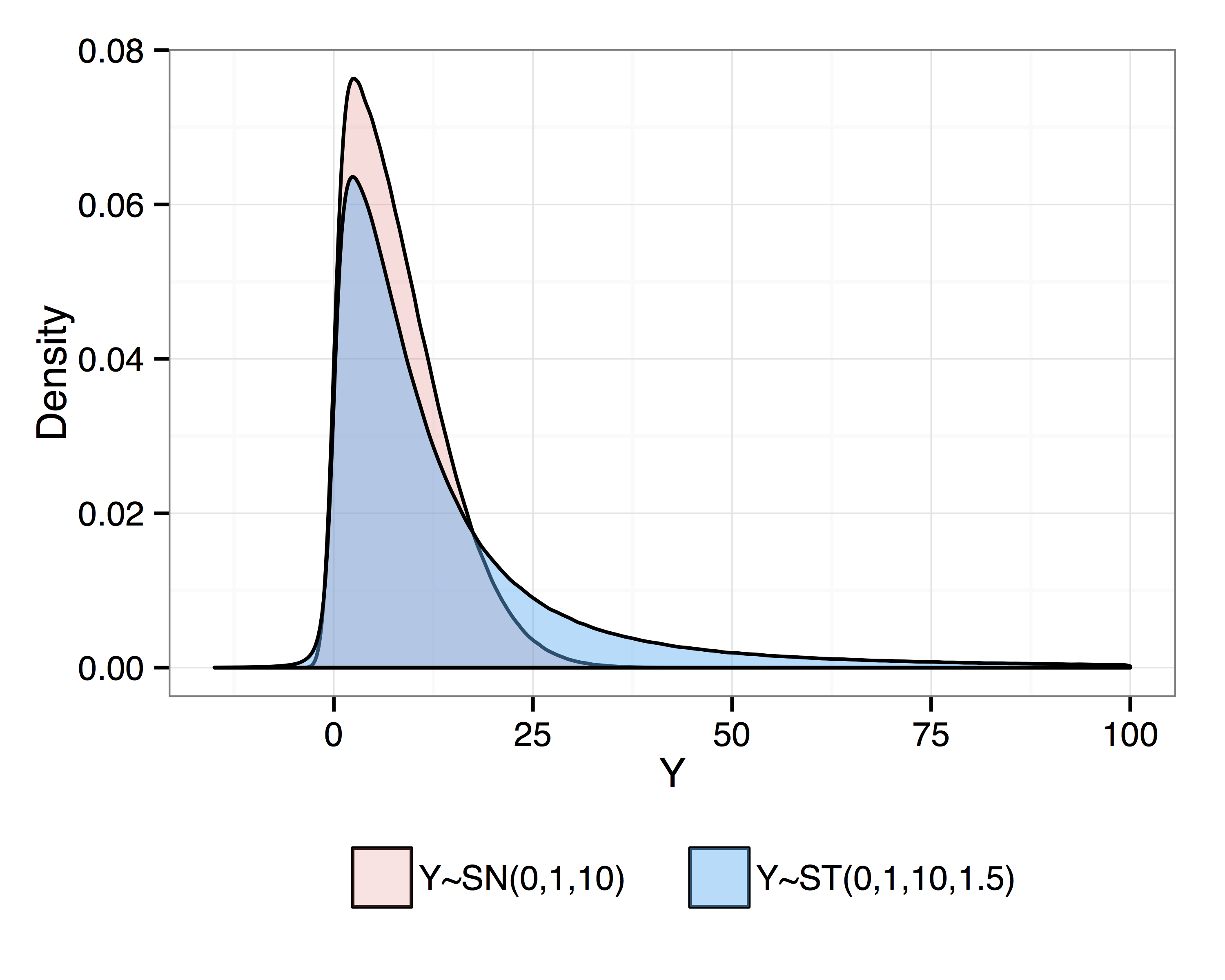
Figure 1: Density probability function of univariate skew Normal $\mathcal{SN}(\xi=0,\psi=10,\sigma=1)$ and skew t $\mathcal{ST}(\xi=0,\psi=10,\sigma=1,\nu=1.5)$ distributions

2.4 Dirichlet process mixture of skew $t$-distribution

Let $G_{0}$ be the base distribution of a Dirichlet process in a DPM combining model (5) with a random-effects model representation (10) of the skew $t$-distribution. $G_{0}$ is the product of a structured Normal inverse Wishart ($sNiW$) and of a prior on $\nu$, the degree of freedom of the skew-t: $G_{0}=sNiW(\xi_{0},\psi_{0},B_{0},\Lambda_{0},\lambda_{0})P_{0,\nu}$. Our proposed model is fully written as follows:

$$\alpha|a,b \sim\text{Gamma}(a,b)$$ (12a)

$$\boldsymbol{\pi}\,\big{|}\,\alpha \sim\text{GEM}(\alpha)$$ (12b)

for $$k=1,2,\ldots$$

$$\boldsymbol{\xi}_{k},\boldsymbol{\psi}_{k},\boldsymbol{\Sigma}_{k},\nu_{k}\ \sim G_{0}$$ (12c)

for $$c=1,2,\ldots,C$$

$$\ell_{c}\,\big{|}\,\boldsymbol{\pi} \sim\text{Mult}(\boldsymbol{\pi})$$ (12d)

$$\gamma_{c}\,\big{|}\,\ell_{c},(\nu_{k}) \sim\text{Gamma}\left(\frac{\nu_{\ell_{c}}}{2},\frac{\nu_{\ell_{c}}}{2}\right)$$ (12e)

$$s_{c}\,\big{|}\,\gamma_{c} \sim\mathcal{N}_{[0,+\infty[}\left(0,\frac{1}{\gamma_{c}}\right)$$ (12f)

$$\boldsymbol{y}_{c}\,\big{|}\,\ell_{c},\gamma_{c},s_{c},(\boldsymbol{\xi}_{k},\boldsymbol{\psi}_{k},\boldsymbol{\Sigma}_{k}) \sim\mathcal{N}\left(\boldsymbol{\xi}_{\ell_{c}}+\boldsymbol{\psi}_{\ell_{c}}s_{c},\frac{1}{\gamma_{c}}\boldsymbol{\Sigma}_{\ell_{c}}\right)$$ (12g)

2.5 Discussion on the model assumptions

In model (12), the base distribution parameter $G_{0}$ conveys the prior information on the cluster parametric shape. For the parameters $\boldsymbol{\xi_{k}}$, $\boldsymbol{\psi_{k}}$ and $\boldsymbol{\Sigma_{k}}$, we have conditional conjugacy with the random-effects model representation using joint priors taking the form of a structured Normal-inverse-Wishart distribution. See Appendix A for details. Frühwirth-Schnatter and Pyne (2010) pointed out that the prior on $\boldsymbol{\Sigma}_{k}$ can have a big impact on the posterior number of clusters. Indeed, setting the scale of the prior on $\boldsymbol{\Sigma}_{k}$ too small will result in an inflated number of clusters in the posterior, whereas too large values tend to cluster all the observations together. Adding a Wishart hyperprior on $\boldsymbol{\Sigma}_{k}$, that carries on conjugacy with the inverse-Wishart, enables us to reduce this impact of the prior (Frühwirth-Schnatter and Pyne, 2010; Huang and Wand, 2013). Assuming prior independence between each $\nu_{k}$ and also from the three parameters mentioned above, we can use any of the three priors proposed in Juárez and Steel (2010) for instance (such as an objective Jeffrey’s prior, see Appendix A).

3 Estimation

3.1 Posterior Estimation via Gibbs sampling

For making inference on the model (12), MCMC methods can be used to sample the partition $\{\ell_{1:C}\}$ and the corresponding cluster parameters $\{\theta^{*}_{k}\}=\left\{\{\boldsymbol{\xi}^{*}_{k}\},\{\boldsymbol{\psi}^{*}_{k}\},\{\boldsymbol{\Sigma}^{*}_{k}\},\{\nu^{*}_{k}\}\right\}$ from the marginal posterior distribution. Extending results from Frühwirth-Schnatter and Pyne (2010) and Caron et al. (2014), it is possible to implement an efficient and valid partially collapsed Gibbs sampler with a Metropolis-Hastings step (van Dyk and Park, 2008; van Dyk and Jiao, 2015). The use of slice sampling (Neal, 2003; Kalli et al., 2011) enables the straightforward parallelization of the latent allocation sampling (thanks to conditional conjugacy) in such an MCMC algorithm (even in the skew-normal and skew-$t$ cases), which can lead to substantial computation speed up when the number of observations $C$ (cells) per sample increases. Each iteration of our Gibbs sampler proceeds in the following order (details are provided Appendix A):

1. Update the concentration parameter $\alpha$ given the previous partition $\{\ell_{1:C}\}$ using the data augmentation technique from Escobar and West (1995).

2. Update the mixing distribution $G$ given $\alpha$, $\{\boldsymbol{\xi}_{k}\}$, $\{\boldsymbol{\psi}_{k}\}$, $\{\boldsymbol{\Sigma}_{k}\}$ and the base distribution $G_{0}$ via slice sampling.

3. For $c=1,\dots,C$ update the individual skew parameter $s_{c}$ given $\{\boldsymbol{\xi}_{k}\}$, $\{\boldsymbol{\psi}_{k}\}$, $\{\boldsymbol{\Sigma}_{k}\}$ and the new $\ell_{c}$.

4. Update $\{\boldsymbol{\xi}_{k}\}$, $\{\boldsymbol{\psi}_{k}\}$, $\{\boldsymbol{\Sigma}_{k}\}$ given the base distribution $G_{0}$, the updated partition $\{\ell_{1:C}\}$ and the updated individual skew parameters $\{s_{1:C}\}$.

5. Finally jointly update the degrees of freedom and the individual scale factors $(\{\nu_{k}\},\{\gamma_{1:C}\})$ in an Metropolis-Hastings (M-H) within Gibbs step. First an M-H step is performed to update the $\{\nu_{k}\}$ where the $\{\gamma_{1:C}\}$ are integrated out, immediately followed by a Gibbs step to sample the $\{\gamma_{1:C}\}$ from their full conditional distribution. This ensures that the reduced conditioning performed in the M-H step does not change the stationary distribution of the Markov chain (van Dyk and Jiao, 2015) – see Appendix A.

3.2 Sequential Posterior Approximation

In flow cytometry experiments it is common to actually have multiple datasets $\boldsymbol{y}^{(i)}$ (with $i=1,\dots,I$) corresponding to multiple individuals, or repeated measurements of the same individual. In such cases, it is of interest to use previous time points or previous samples results as prior information, in order to leverage all the information available to estimate the mixture. However, specifying prior information to Dirichlet process mixture models is not straightforward (Kessler et al., 2015). Here we propose to use the posterior MCMC draws obtained from previous dataset $\boldsymbol{y}^{(i)}$ as prior information to analyze the next dataset $\boldsymbol{y}^{(i+1)}$. To do so, first let’s consider the hierarchical model using all observations from both $\boldsymbol{y}^{(i)}$ and $\boldsymbol{y}^{(i+1)}$ at once :

$$\alpha \sim Gamma(a,b)$$ (13a)

$$G|\alpha \sim DP(\alpha,G_{0})$$ (13b)

$$\boldsymbol{y}^{(i)},\boldsymbol{y}^{(i+1)}|G \overset{\tiny{i.i.d.}}{\sim}\int_{\boldsymbol{\Theta}}f_{\boldsymbol{\theta}}(\cdot)dG(\boldsymbol{\theta})$$ (13c)

We are interested in estimating $p(G|\boldsymbol{y}^{(i)},\boldsymbol{y}^{(i+1)})\propto p(G|\boldsymbol{y}^{(i)})p(\boldsymbol{y}^{(i+1)}|G)$. The idea is to first approximate $p(G|\boldsymbol{y}^{(i)})$ by a Dirichlet process through MCMC draws from the model described in 2.1:

$$p(G|\boldsymbol{y}^{(i)})\simeq\int DP(G;\alpha,G_{1})Gamma(\alpha;a_{1},b_{1})d\alpha$$ (14)

where $G_{1}$, $a_{1}$, $b_{1}$ are parameters to be estimated from the MCMC approximation of the true posterior: i) $\widehat{a_{1}}$ and $\widehat{b_{1}}$ can be taken as MLE estimates from the MCMC samples $\alpha^{(j)}$ ; ii) $\widehat{G_{1}}$ is a parametric approximation of the posterior mixing distribution $G_{1}$ (the true posterior is not suitable for being directly plugged in as a base distribution parameter of another $DP$ as it is nonparametric). In the case of a skew t-distributions mixture model, we approximate $G_{1}$ with the following joint distribution: $G_{1}\simeq(sNiW,P_{0,\nu})$ where $P_{0,\nu}$ is the chosen prior for the skew t-distribution degrees of freedom. To estimate $G_{1}$, we estimate the Maximum a posteriori (MAP) from the posterior MCMC samples (see Appendix B).

Now using this posterior parametric approximation, we have the same hierarchical model as before but conditional on $\boldsymbol{y}^{(i)}$:

$$\alpha|\boldsymbol{y}^{(i)} \sim Gamma(\widehat{a_{1}},\widehat{b_{1}})$$ (15a)

$$G|\alpha,\boldsymbol{y}^{(i)} \sim DP(\alpha,\widehat{G_{1}})$$ (15b)

$$\boldsymbol{y}^{(i+1)}|G,\boldsymbol{y}^{(i)} \overset{\tiny{i.i.d.}}{\sim}\int_{\boldsymbol{\Theta}}f_{\boldsymbol{\theta}}(\cdot)dG(\boldsymbol{\theta})$$ (15c)

Note that under this approximate posterior model, the cluster parameters $\boldsymbol{\theta}_{k}^{*}$ are i.i.d. from $G_{1}$. Such an approach can be iterated a number of times, if for instance several time points are observed, iteratively approximating the successive posteriors. This approach allows to finally account for all the previous information in the mixture model estimation.

3.3 Point estimate of the clustering

Getting a representation of the partition posterior distribution is difficult (Medvedovic and Sivaganesan, 2002). One can use the maximum a posteriori, i.e. using the point estimation form the MCMC sample that maximize the posterior density. However this ignores all the information about the uncertainty around the partition gained through the Bayesian approach.

Another way is to rather consider a co-clustering posterior probability (or similarity) matrix $\zeta$ on each pair $(c,d)$ of observations. Such a matrix can be estimated by averaging the co-clustering matrices from all the explored partitions in the posterior MCMC draws:

$$\widehat{\zeta}_{cd}=\frac{1}{N}\sum_{i=1}^{N}\delta_{\ell_{c}^{(i)}\ell_{d}^{(i)}}$$ (16)

where $N$ is the number of MCMC draws from the posterior and $\delta_{kl}=1$ if $k=l$, $0$ otherwise. An optimal partition point estimate $\{\widehat{\ell}_{1:C}\}$ can then be derived in regard of this similarity matrix through stochastic search with the explored partitions in the posterior MCMC draws (Dahl, 2006), by using a pairwise coincidence loss function (Lau and Green, 2007) such as the one proposed by Binder (1978, 1981) which optimizes the Rand index (Fritsch and Ickstadt, 2009):

$$\{\widehat{\ell}_{1:C}\}=\underset{\{\ell^{(i)}_{1:C}\}\in\left\{\{\ell^{(1)}_{1:C}\},\dots,\{\ell^{(N)}_{1:C}\}\right\}}{\operatorname{arg\,min}}\sum_{c=1}^{C-1}\sum_{d=c+1}^{C}2\left(\delta_{\ell_{c}^{(i)}\ell_{d}^{(i)}}-\widehat{\zeta}_{cd}\right)^{2}$$ (17)

The computational cost of this approach, though, is of the order $\mathcal{O}(NC^{2})$ due to the necessity of computing all the similarity matrices.

A different optimal partition point estimate $\{\tilde{\ell}_{1:C}\}$ can also be derived using the $\mathcal{F}$-measure as our loss function. The $\mathcal{F}$-measure is widely used as a way to summarize the accordance between 2 methods, one being considered as a reference (gold-standard). It is the harmonic mean of the precision and recall:

$$\mathcal{F}=\dfrac{2PrRe}{Pr+Re}$$ (18)

In order to use the $\mathcal{F}$-measure to evaluate our clustering method, we rely on the definition proposed in the online methods from Aghaeepour et al. (2013). In this setting of unsupervised clustering, the precision $Pr$ is the number of cells correctly assigned to a given cluster divided by the total number of cells assigned to that cluster (also called Positive Predictive Value). The recall $Re$ is the number of cells correctly assigned to a given cluster divided by the number of cells that should be assigned to this cluster according to the gold-standard. Since in our problem the labels of the different clusters are exchangeable, the $\mathcal{F}$-measure is computed for each combination of the reference clusters and the predicted clusters. Let $G=\{g_{1},\dots,g_{m}\}$ be a set of $m$ reference clusters and $H=\{h_{1},\dots,h_{n}\}$ be set of $n$ predicted clusters. For each combination pair $(q,r)$ of a reference cluster $g_{q}$ and a predicted cluster $h_{r}$, the $\mathcal{F}$-measure is computed as follows:

$$Pr(h_{r},g_{q})=\dfrac{|g_{q}\cap h_{r}|}{|h_{r}|}\quad\text{and}\quad Pr(h_{r},g_{q})=\dfrac{|g_{q}\cap h_{r}|}{|g_{q}|}$$ (19)

$$\mathcal{F}(h_{r},g_{q})=\dfrac{2Pr(g_{q},h_{r})Re(g_{q},h_{r})}{Pr(g_{q},h_{r})+Re(g_{q},h_{r})}$$ (20)

This $\mathcal{F}$-measure is comprised in $[0,1]$, and the closer it is to 1 the better the agreement is between the predicted cluster and the reference cluster. The total $\mathcal{F}$-measure for a predicted partition $H$ given a gold-standard $G$ is then define as the weighted sum of the best matched $\mathcal{F}$-measure:

$$\mathcal{F}_{tot}(H,G)=\frac{1}{\sum_{q=1}^{m}|g_{q}|}\sum_{q=1}^{m}|g_{q}|\,\underset{r\in\{1,\dots,n\}}{\operatorname{max}}\,\mathcal{F}(h_{r},g_{q})$$ (21)

This total $\mathcal{F}$-measure is again between $0$ and $1$, and the closer it is to 1 the better the predicted partition agrees with the gold-standard. The optimal partition point estimate in respects of this $\mathcal{F}$-measure is then obtained with the partition that maximizes its average $\mathcal{F}$-measure over all the other explored partitions in the posterior MCMC draws:

$$\{\tilde{\ell}_{1:C}\}=\underset{\{\ell^{(i)}_{1:C}\}\in\left\{\{\ell^{(1)}_{1:C}\},\dots,\{\ell^{(N)}_{1:C}\}\right\}}{\operatorname{arg\,max}}\,\frac{1}{N}\sum_{\begin{subarray}{c}j=1\\ j\neq i\end{subarray}}^{N}\mathcal{F}_{tot}\left(\{\ell^{(i)}_{1:C}\},\{\ell^{(j)}_{1:C}\}\right)$$ (22)

Note the $\mathcal{F}$-measure is computed here only between sampled partitions, and a gold-standard partition is unnecessary.

4 Simulations Study

4.1 Non informative prior

First, to assess the performances of the Dirichlet process mixture of skew $t$ distributions model in a simple clustering case, 100 simulations in 2-dimensions were performed. In each simulation 2000 observations were drawn from 4 distinct clusters representing respectively 50%, 30%, 15% and 5% of the data. After 10,000 MCMC iterations (9,000 iterations burnt and a thining of 5 gave 200 partitions sampled from the posterior; the chain was initialized with 30 clusters), the resulting mean $\mathcal{F}$-measure was 0.998 when comparing the partition point estimate obtained from our approach with the true clustering of the simulated data. In 97% of the cases, the partition point estimate had 4 clusters (i.e. the true number of clusters in the simulated data), while it had 3 or 5 clusters in the remaining 3%. Figure 2 shows an example of the partition point estimate obtained for one of those simulation run.

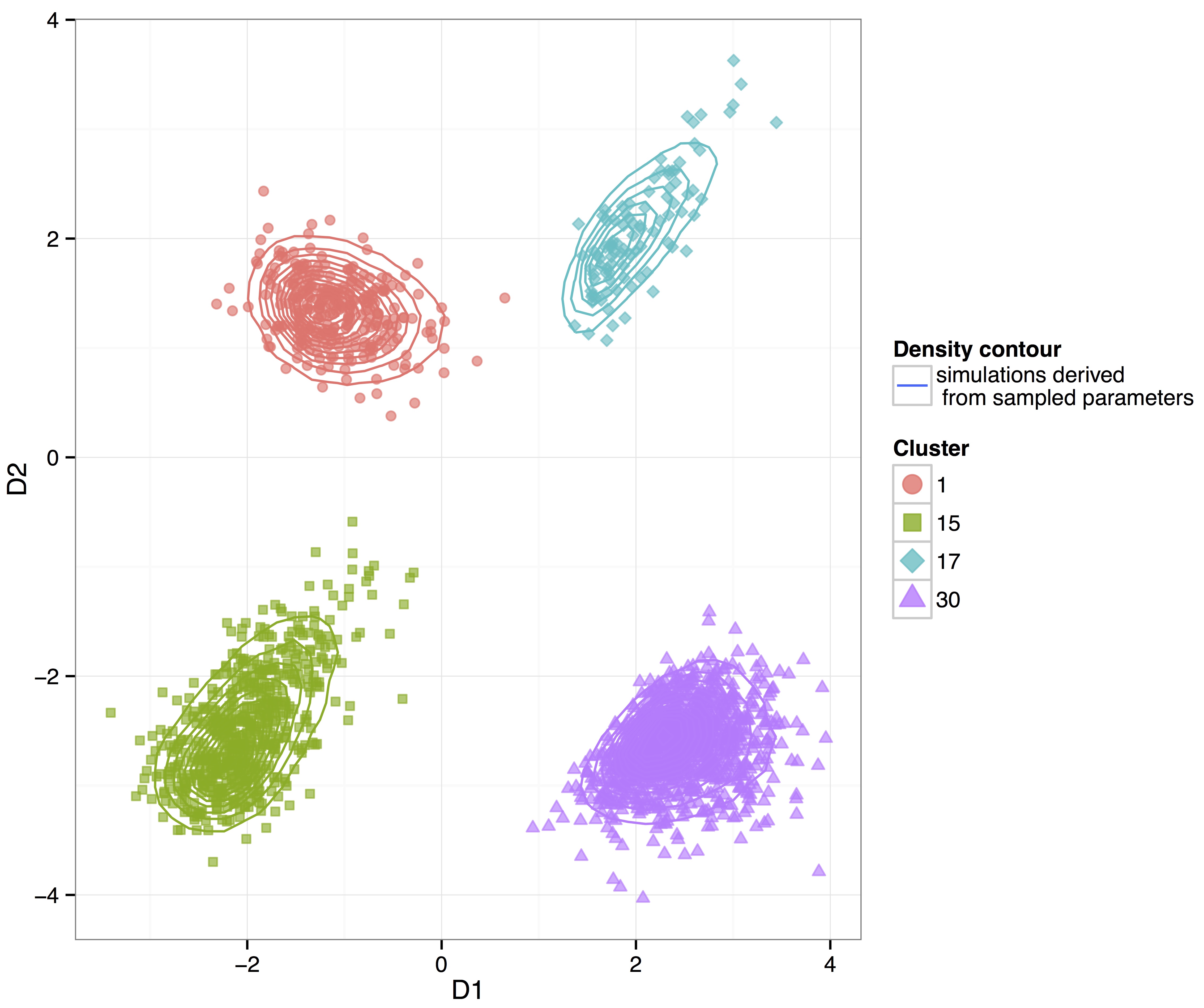
Figure 2: Partition point estimate from one of the first 100 2-dimensional simulations

4.2 Sequential posterior approximation plugged-in as informative prior

To illustrate how the sequential posterior approximation strategy compares to the standard non informative prior setting, we ran simulations where we considered two samples derived from the same infinite mixture model. The first sample is simulated for a time $t$, and the second sample at $t+1$. As all observations originate from the exact same distribution, regardless of the sample, the hypothesis of the sequential posterior approximation strategy is satisfied. One of the major gain observed is the time to convergence for the partition. Using an informative prior derived from the sample at time $t$ to estimate the partition of the sample from $t+1$ makes it more than three time faster to converge according to the Gelman-Rubin statistics.

In further simulations, we also investigated the performance of this sequential posterior approximation strategy. As opposed to using the standard non informative prior, it shows substantial gains when the amount of information brought by the prior is substantial compared to the amount available from the data at $t+1$ alone. As the amount of information available at $t+1$ increases, the gain from using this strategy can become less noticeable, as shown using the $\mathcal{F}$-measure in Figure 3. But even when as many observations are available at $t+1$ as at $t$, the accuracy for rare cell populations is still improved by using an informative prior. This is not necessary visible at the scale of the total $\mathcal{F}$-measure, because it is masked by the larger clusters. However, when computing a limited $\mathcal{F}$-measure, that only takes into account smaller clusters (see Appendix C), the use of an informative prior in this sequential strategy seems to always improves the clustering accuracy for smaller clusters (see Supplementary Figure S1 in Appendix C).

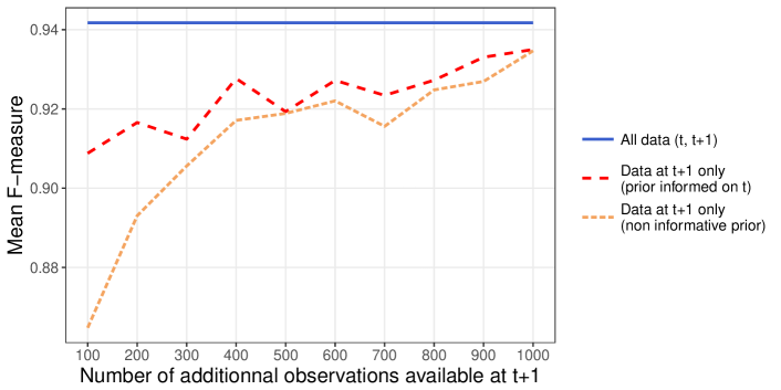
Figure 3: Mean $\mathcal{F}$-measure according to the number of observations available at $t+1$, while 1,000 observations are available at $t$, over 300 simulations

5 Application to real datasets

5.1 Benchmark Graft versus Host Disease dataset

The Graft versus Host Disease (GvHD) dataset is a public dataset that was first analysed (manually gated) in Brinkman et al. (2007), with the objective of identifying cellular signature that correlates or predict Graft versus Host disease. The GvHD data were used as benchmark data in the FlowCAP challenge Aghaeepour et al. (2013). Flow cytometry data was collected for 12 sample, and original manual gates are being regarded as the true cell clustering (actually a consensus over eight manual operators, from eight different operators). In order to try to mitigate further the well known reproducibility issues with manual gating (Ge and Sealfon, 2012; Aghaeepour et al., 2013), only the most concordant clusters between the 8 gatings ($\mathcal{F}$-measure above 0.8) were used for comparing with the automated results, as was done in Aghaeepour et al. (2013). The data were downloaded from the FlowCAP project website [http://flowcap.flowsite.org/] as part of the FlowCAP-I challenge [http://flowcap.flowsite.org/codeanddata/FlowCAP-I.zip]. Table 1 shows the performance of our proposed approach NPflow on this dataset, in the context of the other approaches reviewed by Aghaeepour et al. (2013). The $\mathcal{F}$-measure is computed for all samples available for a given dataset and the mean over all samples is reported, as well as bootstrap 95% Confidence Intervals. No algorithm is performing significantly better than NPflow thus placing NPflow among the top methods for automatic gating, and the sequential approach yields a $\mathcal{F}$-measure higher than any other method.

Table 1: Mean $\mathcal{F}$-measures across all the 12 samples from the GvHD benchmark dataset

Method	$\mathcal{F}$-measure
NPflow	0.85 (0.80, 0.90)
NPflow-seq	0.89 (0.85, 0.94)
ADICyt	0.81 (0.72, 0.88)
CDP	0.52 (0.46, 0.58)
FLAME	0.85 (0.77, 0.91)
FLOCK	0.84 (0.76, 0.90)
flowClust/Merge	0.69 (0.55, 0.79)
flowMeans	0.88 (0.82, 0.93)
FlowVB	0.85 (0.79, 0.91)
L2kmeans	0.64 (0.57, 0.72)
MM	0.83 (0.74, 0.91)
MMPCA	0.84 (0.74, 0.93)
SamSPECTRAL	0.87 (0.81, 0.93)
SWIFT	0.63 (0.56, 0.70)

All estimates except for our proposed NPflow approach are from Aghaeepour et al. (2013). 95% Confidence Intervals are calculated on 10,000 bootstrap samples of the $\mathcal{F}$-measures.

The GvHD benchmark data are not longitudinal data. However, the sequential posterior model can still improve the results by using each individual sample sequentially. Using this dataset, the mean $\mathcal{F}$-measure reached 0.89 (0.85, 0.94) with the sequential approach, compared to a value of 0.85 (0.80, 0.90) with the standard NPflow model (Table 1). The sequential strategy exhibits the highest $\mathcal{F}$-measure for the GvHD dataset, making it the best approach for unsupervised automatic gating compared to competing methods evaluated in Aghaeepour et al. (2013).

5.2 Original DALIA-1 data

We also applied our method to an original dataset from DALIA-1, a phase I trial evaluating a therapeutic vaccine against HIV (Lévy et al., 2014). The vaccine candidate was based on ex-vivo generated interferon-$\alpha$ dendritic cells loaded with HIV-1 lipo-peptides, and activated with lipopolysaccharide. The objectives of the trial were to evaluate the safety of the strategy and to evaluate the immune response to the vaccine. For our purpose here, we are interested in the 12 HIV positive patients who had their cellular populations quantified at 18 time-points during the trial. More specifically, we focused on two time points (at week 24 and week 26 of the trial) immediately following antiretroviral treatment (HAART) interruption which took place at week 24. Following this interruption, the increase of viral replication is associated with changes in cell populations (Thiébaut et al., 2005; Lévy et al., 2012). Here we especially looked at the effector CD4+ T-cells, defined as CD45RA+CD27- among the CD3+CD4+ cells (Larbi and Fulop, 2014), that are one of the first cell populations to be affected during the viral rebound (Lévy et al., 2012). Since flow-cytometry measurements were repeated at each time points for each patients, we used the sequential strategy at week 26, in the hope to use the information from week 24 to better identify the effector CD4+ T-cell population at the next time point. Figure 4 illustrates the overall efficiency gain at week 26 from using the sequential strategy. The average limited $\mathcal{F}$-measure (compared to available manual gating used as gold-standard) on those 12 samples is $0.5$ for NPflow with a non-informative prior, and increase to $0.59$ with the sequential strategy. By comparison, flowMeans (the second best method on the GvHD dataset) gives an average limited $\mathcal{F}$-measure of $0.51$ (see Appendix D for details). Figure 5 gives an example of a patient for which the sequential strategy was especially improving the identification of the effector CD4+ T-cells. In this case, the percentage of effector CD4+ T-cells was estimated at 31.7 by the manual gating, at 7.5 by NPflow, and at 38.1 by the sequential strategy. Figure 6 shows the general increase of effector CD4+ T-cell proportions for every patients after treatment interruption (see Appendix D for more details).

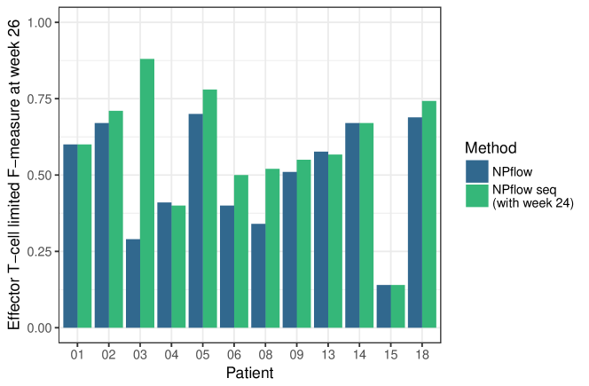
Figure 4: Limited $\mathcal{F}$-measures for the effector CD4+ T-cell population from the DALIA-1 trial two weeks after HAART interruption for NPflow with or without the sequential strategy, compared to manual gating.

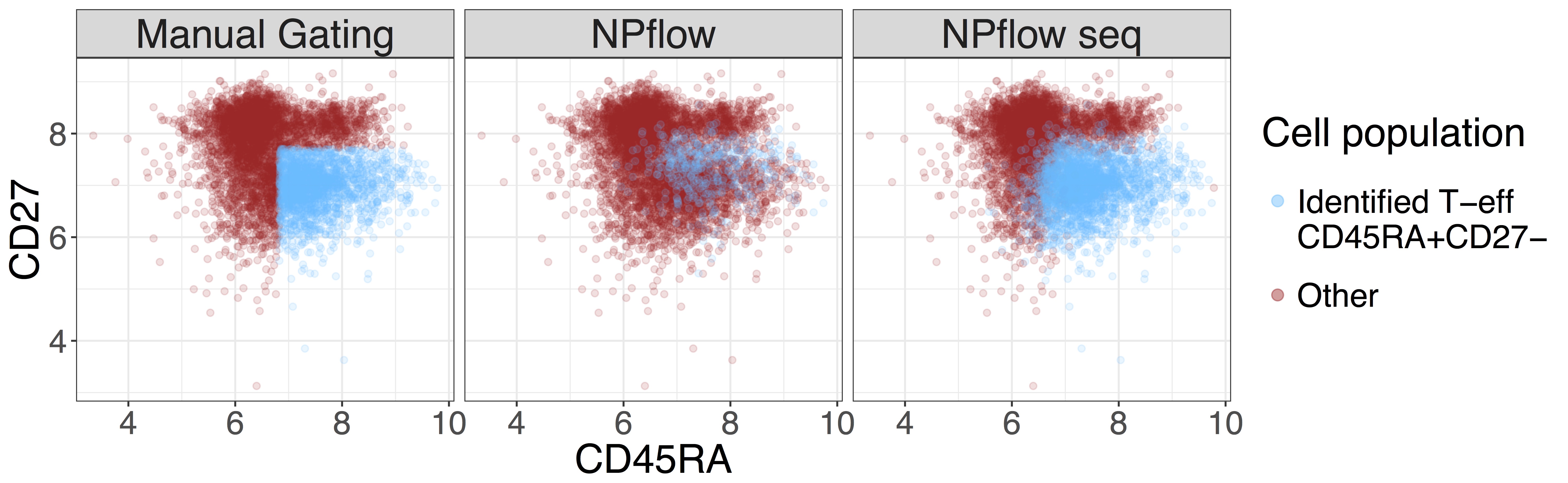
Figure 5: CD3+CD4+ cells of patient 3 from the DALIA-1 trial two weeks after HAART interruption (at week 26).

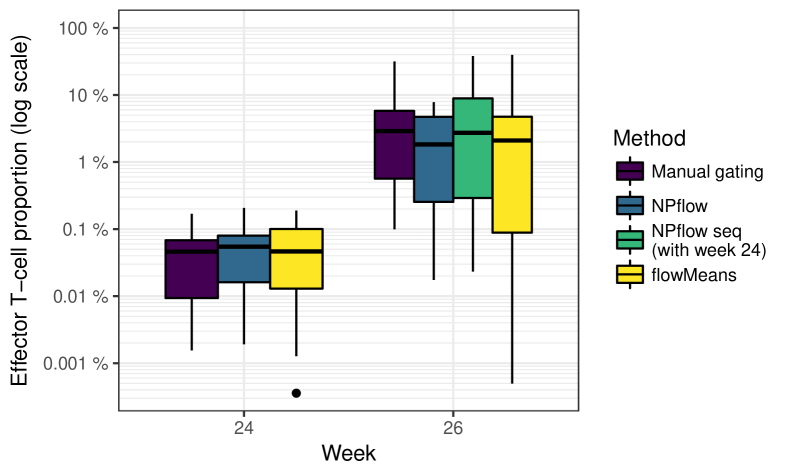
Figure 6: Evolution of the proportion of effector CD4+ T-cells in the DALIA-1 trial following HAART interruption (from manual gating).

In addition to providing a point estimate of the partition, our method also quantifies the uncertainty around the posterior clustering through posterior co-clustering probabilities. Figure 7 displays such a co-clustering posterior probabilities matrix. Where we can clearly identify 4 core clusters, with some uncertainty corresponding to marginal cells that are in between overlapping populations.

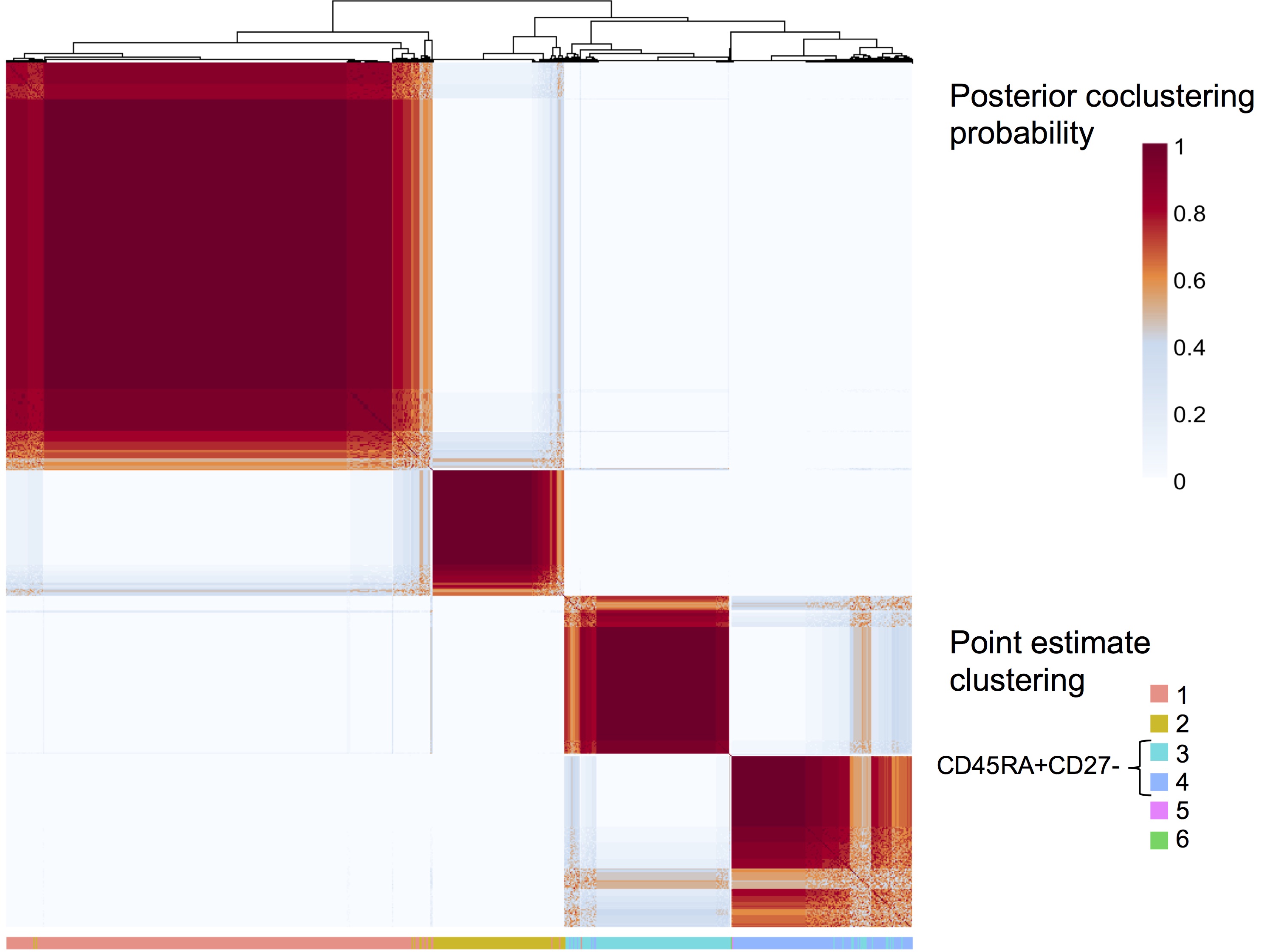
Figure 7: Heatmap of the posterior co-clustering probabilities for the CD3+CD4+ cells of patient 3 at week 26 from DALIA-1.

6 Discussion

We extend the classical Dirichlet process Gaussian mixture model to skew t-distribution mixtures, based on Frühwirth-Schnatter and Pyne (2010) parametrization of such distributions. Such an approach is well suited for unsupervised model based classification of flow cytometry data. Automatic gating of cell populations is an open research problem and the proposed approach features two important characteristics for this task: i) it avoids the difficult issue of model selection by estimating directly the number of components in the mixture ; ii) it uses skew and heavy tailed distributions in the form of skew t-distributions, of which the gaussian is a particular case. Estimation of the posterior co-clustering probabilities for each data pair allows to quantify the uncertainty about the posterior partition, and an optimal point estimate of the clustering is provided by minimizing a cost function in regards to the average posterior co-clustering matrix. We have developed and implemented an efficient collapsed Metropolis within Gibbs sampler for estimating such models. One of the advantage of our proposed sampler is the absence of label switching issue, as it uses directly the partition of the data without having to deal with labels (Jasra et al., 2005). As an indication of runtime, around 3,000 MCMC iterations can be run on average for a real dataset of around 10,000 observations over 6 dimensions, using one Intel® Xeon® x5675 processor in an hour. Besides, instead of using a partially collapse Gibbs sampler algorithm, it could be of interest to also investigate the use of sequential Monte-Carlo algorithms, especially for the sequential modeling strategy or other possible dynamic extensions of the model proposed here (Caron et al., 2008, 2017).

We propose to use sequential parametric approximations of the posterior as refined informative priors in case of repeated measurement of flow cytometry data. The proposed sequential analysis strategy enables to analyze each sample sequentially, as the data are acquired. It does not require to wait for the last sample to perform the automatic gating nor to analyze all data at once, but it still uses available prior knowledge. This contrasts with hierarchical extensions of the Dirichlet Process Mixture Model such as those proposed by Cron et al. (2013) or Dundar et al. (2014), where the complete dataset must be analyzed at once. This sequential strategy allows one to analyze the samples as they are acquired, which can be useful in clinical trials where there are often intermediate analyses for instance. Moreover in large studies the size of the data can make it challenging to analyze all samples at once, and such a sequential approach then makes practical sense (Huang and Gelman, 2005). Futhermore, this use of sequentially informed priors does not face the usual complications of cluster matching arising when an algorithm is run on each sample separately (Cron et al., 2013). In our simulation study this sequential posterior approximation strategy improves the fit of the model. In addition, such a strategy exhibits accelerated convergence and greater accuracy for small clusters, as long as the different samples are similar enough. Besides, the parametric prior can also be specified to inform the model with expert knowledge, e.g. to favor a range for the expected number of clusters. On real flow-cytometry data we show that the sequential strategy also improves the clustering performances. On the benchmark GvHD dataset, it outperforms all other methods investigated in by Aghaeepour et al. (2013). In the DALIA-1 trial, the sequential strategy allows a better recovery of the effector CD4+ T-cell population after a important perturbation of this targeted population following HAART interruption among HIV positive patients. It is worth noting however that in other cases, for instance if the data distributions were too different from samples to samples, the sequential posterior model would not necessarily improve the clustering results, and could even gave a diminished $F$-measure compared to the non sequential strategy.

Manual gating is still considered the gold-standard when evaluating an automatic gating strategy on real flow cytometry data. Yet one should keep in mind that manual gating has reproducibility issues, often resulting in a partial and subjective clustering (Ge and Sealfon, 2012; Welters et al., 2012; Aghaeepour et al., 2013; Gondois-Rey et al., 2016). Therefore using manual gating as the gold-standard might not be actually the best way to assess the performance of automatic gating algorithms on real data, because of its inherent flaws.

Mass cytometry is a technology very similar to flow cytometry. Using ions in place of colors, CyTOF is able to measure up to 40 cell markers at once, generating even more data than flow cytometry. Efficient automated gating method are therefore all the more needed in the context of CyTOF(Melchiotti et al., 2017). The approach proposed here could be directly applied to such data. More generally, we propose here a framework for Dirichlet process mixtures of multivariate skew t-distributions modeling that is suitable for any kind of data modeled as such a mixture, especially when the number of mixture component is unknown. We provide an efficient implementation of our method within the R package NPflow that is available on CRAN at https://cran.r-project.org/web/packages/NPflow.

Software

Software in the form of R code is available on the Comprehensive R Archive Network as an R package tcgsaseq.

Appendix

A Gibbs samplers

• $K$ is the number of different unique values taken by $c$ (i.e. the number of clusters). This number of clusters $K$ is not set and its value may change at each iteration.

• $\ell_{c}$ is the latent variable indicating which cluster the observation $c$ belongs to. $\{\ell_{1:C}\}$ refers to a whole partition of the data.

• $s_{c}$ is the skew parameter for the observation $c$.

• $\gamma_{c}$ is the scale parameter (skew t only) for the observation $c$.

A.1 Skew Normal distributions mixture

Our Gibbs sampler proceeds with each of the following updates in turn:

1. update concentration parameter $\alpha$ given $\{\ell_{1:C}\}$ using the data augmentation technique from West (1992):
   $\alpha\propto p(\alpha|\{\boldsymbol{z}_{1:C}\},G_{0},\{\boldsymbol{\xi}_{k}\},\{\boldsymbol{\psi}_{k}\},\{\boldsymbol{\Sigma}_{k}\},\{\ell_{1:C}\},\{w_{k}\},\{s_{1:C}\})\propto p(\alpha|\{\ell_{1:C}\})$
   $(\alpha,x|\{\ell_{1:C}\})\sim p(\alpha)\alpha^{K-1}(\alpha+C)x^{\alpha}(1-x)^{C-1}$
   $(x|\alpha,\{\ell_{1:C}\})\sim\text{Beta}(\alpha+1,C)$
   $(\alpha|x,\{\ell_{1:C}\})\sim\pi_{x}\text{Gamma}(a+K,b-\log(x))+(1-\pi_{x})\text{Gamma}(a+K-1,b-\log(x))$ with $p(\alpha)\propto\text{Gamma}(a,b)$ and $\frac{\pi_{x}}{1-\pi_{x}}=\frac{a+k-1}{C(b-\log(x))}$

2. update $G$ given $\alpha$, $\{\boldsymbol{\xi}_{k}\}$, $\{\boldsymbol{\psi}_{k}\}$, $\{\boldsymbol{\Sigma}_{k}\}$ and $G_{0}$ via slice sampling:
   $\{w_{k}\},\{\ell_{1:C}\}\propto p\left(\{w_{k}\},\{\ell_{1:C}\}|\{\boldsymbol{z}_{1:C}\},\alpha,G_{0},\{\boldsymbol{\xi}_{k}\},\{\boldsymbol{\psi}_{k}\},\{\boldsymbol{\Sigma}_{k}\},\{s_{1:C}\}\right)$

   1. sample the weights:
      $(w_{1},\dots,w_{K},w_{*}|\{\ell_{1:C}\})\sim\text{Dirichlet}(\text{card}(\{\ell_{c}=1\}),\dots,\text{card}(\{\ell_{c}=K\}),\alpha)$

   2. for $c=1,\dots,C$: $u_{c}\sim\text{Unif}([0,w_{\ell_{c}}[)$

   3. Set $j=K$. While $\sum_{k=1}^{j}w_{k}<(1-min(u_{1:C}))$:

      • set $j=j+1$

      • sample $\pi_{j}\sim\text{Beta}(1,\alpha)$

      • set $w_{j}=w_{*}\pi_{j}\prod_{k={K+1}}^{j-1}(1-\pi_{k})$

      • sample $(\boldsymbol{\xi}_{j},\boldsymbol{\psi}_{j},\boldsymbol{\Sigma}_{j}|G_{0})\sim G_{0}$

   4. for $c=1,\dots,C$ sample $\ell_{c}$ given $\{\boldsymbol{\xi}_{k}\}$, $\{\boldsymbol{\psi}_{k}\}$, $\{\boldsymbol{\Sigma}_{k}\}$, $\{w_{k}\}$ from:
      $p(\ell_{c}=k)\propto\mathds{1}_{\{w_{k}>u_{c}\}}f_{\mathcal{SN}}(\boldsymbol{z}_{c},\boldsymbol{\xi}_{k},\boldsymbol{\psi}_{k},\boldsymbol{\Sigma}_{k})$

3. for $c=1,\dots,C$ update $s_{c}$ given $\ell_{c}$ , $\{\boldsymbol{\xi}_{k}\}$, $\{\boldsymbol{\psi}_{k}\}$, $\{\boldsymbol{\Sigma}_{k}\}$:
   $p(s_{c}|\boldsymbol{z}_{c},\alpha,G_{0},\{\boldsymbol{\xi}_{k}\},\{\boldsymbol{\psi}_{k}\},\{\boldsymbol{\Sigma}_{k}\},\{\ell_{1:C}\},\{w_{k}\})$ $\propto p(s_{c}|\boldsymbol{z}_{c},\{\boldsymbol{\xi}_{k}\},\{\boldsymbol{\psi}_{k}\},\{\boldsymbol{\Sigma}_{k}\},\ell_{c})$
   $(s_{c}|\boldsymbol{z}_{c},\{\boldsymbol{\xi}_{k}\},\{\boldsymbol{\psi}_{k}\},\{\boldsymbol{\Sigma}_{k}\},\ell_{c})\sim\mathcal{N}_{[0,+\infty[}(a_{c},A_{c})$
   with $A_{c}=\frac{1}{1+\boldsymbol{\psi}_{\ell_{c}}^{\prime}\boldsymbol{\Sigma}_{\ell_{c}}^{-1}\boldsymbol{\psi}_{\ell_{c}}}$ and $a_{c}=A_{c}\boldsymbol{\psi}_{\ell_{c}}^{\prime}\boldsymbol{\Sigma}_{\ell_{c}}^{-1}(\boldsymbol{z}_{c}-\boldsymbol{\xi}_{\ell_{c}})$

4. for $k=1,\dots,K$ update $\boldsymbol{\xi}_{k}$, $\boldsymbol{\psi}_{k}$ and $\boldsymbol{\Sigma}_{k}$ given $G_{0}$, $\{\ell_{1:C}\}$ and $\{s_{1:C}\}$ from
   $p(\{\boldsymbol{\xi}_{k}\},\{\boldsymbol{\psi}_{k}\},\{\boldsymbol{\Sigma}_{k}\}|\{\boldsymbol{z}_{1:C}\},\alpha,G_{0},\{\ell_{1:C}\},\{w_{k}\},\{s_{1:C}\})$:

   1. update $G_{k}$ given $\{\boldsymbol{z}_{1:C}\}$, $G_{0}$, $\{\ell_{1:C}\}$ and $\{s_{1:C}\}$:

      • $G_{0}=sNiW(\boldsymbol{b}_{0}^{\xi},\,\boldsymbol{b}_{0}^{\psi},\boldsymbol{B}_{0},\boldsymbol{\Lambda}_{0},\lambda_{0})$ with $\boldsymbol{b}_{0}=(\boldsymbol{b}_{0}^{\xi}\,{}^{\prime}\,\boldsymbol{b}_{0}^{\psi}\,{}^{\prime})^{\prime}$ and $\boldsymbol{B}_{0}=diag(D_{0}^{\xi},\,D_{0}^{\psi})$

      • $G_{k}=sNiW(\boldsymbol{b}_{k}^{\xi},\,\boldsymbol{b}_{k}^{\psi},\boldsymbol{B}_{k},\boldsymbol{\Lambda}_{k},\lambda_{k})$ with $\boldsymbol{b}_{k}=(\boldsymbol{b}_{k}^{\xi}\,{}^{\prime}\,\boldsymbol{b}_{k}^{\psi}\,{}^{\prime})^{\prime}$

      • let $\boldsymbol{X}_{k}$ be a matrix of dimension $\text{card}(\{c|\ell_{c}=k\})\times 2$: $\boldsymbol{X}_{k}=(\boldsymbol{1}\ s_{c|\ell_{c}=k})$

      • let $\boldsymbol{B}_{k}=(\boldsymbol{X}_{k}^{\prime}\boldsymbol{X}_{k}+diag(\boldsymbol{D}_{0})^{-1})^{-1}$

      • $\boldsymbol{b}_{k}=\left(z_{c|\ell_{c}=k}\,\boldsymbol{X}_{k}+\left(\frac{1}{D_{0}^{\xi}}\boldsymbol{b}_{0}^{\xi}\ \frac{1}{D_{0}^{\psi}}\boldsymbol{b}_{0}^{\psi}\right)\right)\boldsymbol{B}_{k}$

      • $\lambda_{k}=\lambda_{0}+\text{card}(\{c|\ell_{c}=k\})$

      • $\displaystyle\boldsymbol{\Lambda}_{k}=\boldsymbol{\Lambda}_{0}+\sum_{c|\ell_{c}=k}\boldsymbol{\varepsilon}_{c}\boldsymbol{\varepsilon}_{c}^{\prime}+\frac{1}{D_{0}^{\xi}}(\boldsymbol{b}_{k}^{\xi}-\boldsymbol{b}_{0}^{\xi})(\boldsymbol{b}_{k}^{\xi}-\boldsymbol{b}_{0}^{\xi})^{\prime}+\frac{1}{D_{0}^{\psi}}(\boldsymbol{b}_{k}^{\psi}-\boldsymbol{b}_{0}^{\psi})(\boldsymbol{b}_{k}^{\psi}-\boldsymbol{b}_{0}^{\psi})$
        with $\boldsymbol{\varepsilon}_{c}=\boldsymbol{z}_{c}-\boldsymbol{b}_{k}^{\xi}-s_{c}\boldsymbol{b}_{k}^{\psi}$

   2. sample $(\boldsymbol{\xi}_{k},\boldsymbol{\psi}_{k},\boldsymbol{\Sigma}_{k}|G_{k})\sim G_{k}$

      • $((\boldsymbol{\xi}_{k},\boldsymbol{\psi}_{k})|\boldsymbol{\Sigma}_{k},\{\ell_{1:C}\},\{s_{1:C}\},G_{k})\sim\mathcal{N}_{2d}\left((\boldsymbol{b}_{k}^{\xi},\boldsymbol{b}_{k}^{\psi}),\boldsymbol{B}_{k}\otimes\boldsymbol{\Sigma}_{k}\right)$

      • $(\boldsymbol{\Sigma}_{k}|\{\ell_{1:C}\},\{s_{1:C}\},G_{k})\sim\mathcal{W}^{-1}(\lambda_{k},\boldsymbol{\Lambda}_{k})$

A.2 Skew $t$-distributions mixture

Our Gibbs sampler for non parametric skew $t$-distributions mixture proceeds with each of the following updates in turn:

1. update concentration parameter $\alpha$ given $\{\ell_{1:C}\}$ using the data augmentation technique from West (1992):
   $\alpha\propto p(\alpha|\{\boldsymbol{z}_{1:C}\},G_{0},\{\boldsymbol{\xi}_{k}\},\{\boldsymbol{\psi}_{k}\},\{\boldsymbol{\Sigma}_{k}\},\{\nu_{k}\},\{\ell_{1:C}\},\{w_{k}\},\{s_{1:C}\},\{\gamma_{1:C}\})\propto p(\alpha|\{\ell_{1:C}\})$
   $(\alpha,x|\{\ell_{1:C}\})\sim p(\alpha)\alpha^{K-1}(\alpha+C)x^{\alpha}(1-x)^{C-1}$
   $(x|\alpha,\{\ell_{1:C}\})\sim\text{Beta}(\alpha+1,C)$
   $(\alpha|x,\{\ell_{1:C}\})\sim\pi_{x}\text{Gamma}(a+K,b-\log(x))+(1-\pi_{x})\text{Gamma}(a+K-1,b-\log(x))$ with $p(\alpha)\propto\text{Gamma}(a,b)$ and $\frac{\pi_{x}}{1-\pi_{x}}=\frac{a+k-1}{C(b-\log(x))}$

2. update $G$ given $\alpha$, $\{\boldsymbol{\xi}_{k}\}$, $\{\boldsymbol{\psi}_{k}\}$, $\{\boldsymbol{\Sigma}_{k}\}$, $\{\nu_{k}\}$ and $G_{0}$ via slice sampling:
   $\{w_{k}\},\{\ell_{1:C}\}\propto p(\{w_{k}\},\{\ell_{1:C}\}|\{\boldsymbol{z}_{1:C}\},\alpha,G_{0},\{\boldsymbol{\xi}_{k}\},\{\boldsymbol{\psi}_{k}\},\{\boldsymbol{\Sigma}_{k}\},\{\nu_{k}\},\{s_{1:C}\},\{\gamma_{1:C}\})$

   1. sample the weights:
      $(w_{1},\dots,w_{K},w_{*}|\{\ell_{1:C}\})\sim\text{Dirichlet}\left(\text{card}(\{\ell_{1:C}\}=1),\dots,\text{card}(\{\ell_{1:C}\}=K),\alpha\right)$

   2. for $c=1,\dots,C$: $u_{c}\sim\text{Unif}([0,w_{\ell_{c}}])$

   3. Set $j=K$. While $\sum_{k=1}^{j}w_{k}<(1-min(u_{1:C}))$:

      • set $j=j+1$

      • sample $\pi_{j}\sim\text{Beta}(1,\alpha)$

      • set $w_{j}=w_{*}\pi_{j}\prod_{k={K+1}}^{j-1}(1-\pi_{k})$

      • sample $(\boldsymbol{\xi}_{j},\boldsymbol{\psi}_{j},\boldsymbol{\Sigma}_{j}|G_{0})\sim\text{structured-Normal-invWishart}(G_{0})$

      • sample $\nu_{j}\sim p(\nu_{j})$

   4. $K=j$

   5. for $c=1,\dots,C$ sample $\ell_{c}$ given $\{\boldsymbol{\xi}_{k}\}$, $\{\boldsymbol{\psi}_{k}\}$, $\{\boldsymbol{\Sigma}_{k}\}$, $\{w_{k}\}$ from:
      $p(\ell_{c}=k)\propto\mathds{1}_{\{w_{k}>u_{c}\}}f_{\mathcal{SN}}(\boldsymbol{z}_{c},\boldsymbol{\xi}_{k},\boldsymbol{\psi}_{k},\boldsymbol{\Sigma}_{k})$

3. for $c=1,\dots,C$ update $s_{c}$ given $\ell_{c}$ , $\{\boldsymbol{\xi}_{k}\}$, $\{\boldsymbol{\psi}_{k}\}$, $\{\boldsymbol{\Sigma}_{k}\}$:
   $(s_{c}|\boldsymbol{z}_{c},\{\boldsymbol{\xi}_{k}\},\{\boldsymbol{\psi}_{k}\},\{\boldsymbol{\Sigma}_{k}\},\ell_{c})\sim\mathcal{N}_{[0,+\infty[}(a_{c},A_{c})$
   with $A_{c}=\frac{1}{1+\boldsymbol{\psi}_{\ell_{c}}^{\prime}\boldsymbol{\Sigma}_{\ell_{c}}^{-1}\boldsymbol{\psi}_{\ell_{c}}}$ and $a_{c}=A_{c}\boldsymbol{\psi}_{\ell_{c}}^{\prime}\boldsymbol{\Sigma}_{\ell_{c}}^{-1}(\boldsymbol{z}_{c}-\boldsymbol{\xi}_{\ell_{c}})$

4. for $k=1,\dots,K$ update $\boldsymbol{\xi}_{k}$, $\boldsymbol{\psi}_{k}$ and $\boldsymbol{\Sigma}_{k}$ given $G_{0}$, $\{\ell_{1:C}\}$ and $\{s_{1:C}\}$ from:
   $p(\{\boldsymbol{\xi}_{k}\},\{\boldsymbol{\psi}_{k}\},\{\boldsymbol{\Sigma}_{k}\}|\{\boldsymbol{z}_{1:C}\},\alpha,G_{0},\{\nu_{k}\},\{\ell_{1:C}\},\{w_{k}\},\{s_{1:C}\},\{\gamma_{1:C}\})$
   $\propto p(\{\boldsymbol{\xi}_{k}\},\{\boldsymbol{\psi}_{k}\},\{\boldsymbol{\Sigma}_{k}\}|\{\ell_{1:C}\},\{s_{1:C}\},G_{0})$:

   1. update the hyper parameters of the cluster distribution given $\{\boldsymbol{z}_{1:C}\}$, $G_{0}$, $\{\ell_{1:C}\}$ and $\{s_{1:C}\}$:

      • $G_{0}=sNiW(\boldsymbol{b}_{0}^{\xi},\,\boldsymbol{b}_{0}^{\psi},\boldsymbol{B}_{0},\boldsymbol{\Lambda}_{0},\lambda_{0})$ with $\boldsymbol{b}_{0}=vec(\boldsymbol{b}_{0}^{\xi},\,\boldsymbol{b}_{0}^{\psi})$ and $\boldsymbol{B}_{0}=diag(D_{0}^{\xi},\,D_{0}^{\psi})$

      • $G_{k}=sNiW(\boldsymbol{b}_{k}^{\xi},\,\boldsymbol{b}_{k}^{\psi},\boldsymbol{B}_{k},\boldsymbol{\Lambda}_{k},\lambda_{k})$ with $\boldsymbol{b}_{k}=vec(\boldsymbol{b}_{k}^{\xi},\,\boldsymbol{b}_{k}^{\psi})$

      • let $\boldsymbol{X}_{k}$ be a matrix of dimension $\text{card}(\{c|\ell_{c}=k\})\times 2$: $\boldsymbol{X}_{k}=(\boldsymbol{1}\ s_{c|\ell_{c}=k})$

      • let $\boldsymbol{B}_{k}=(\boldsymbol{X}_{k}^{\prime}\boldsymbol{X}_{k}+(\boldsymbol{B}_{0})^{-1})^{-1}$

      • $\boldsymbol{b}_{k}=\left(z_{c|\ell_{c}=k}\,\boldsymbol{X}_{k}+\left(\frac{1}{D_{0}^{\xi}}\boldsymbol{b}_{0}^{\xi}\ \frac{1}{D_{0}^{\psi}}\boldsymbol{b}_{0}^{\psi}\right)\right)\boldsymbol{B}_{k}$

      • $\lambda_{k}=\lambda_{0}+\text{card}(\{\ell_{c}=k\})$

      • $\boldsymbol{\Lambda}_{k}=\boldsymbol{\Lambda}_{0}+\displaystyle{\sum_{c|\ell_{c}=k}}\boldsymbol{\varepsilon}_{c}\boldsymbol{\varepsilon}_{c}^{\prime}+\frac{1}{D_{0}^{\xi}}(\boldsymbol{b}_{k}^{\xi}-\boldsymbol{b}_{0}^{\xi})(\boldsymbol{b}_{k}^{\xi}-\boldsymbol{b}_{0}^{\xi})^{\prime}+\frac{1}{D_{0}^{\psi}}(\boldsymbol{b}_{k}^{\psi}-\boldsymbol{b}_{0}^{\psi})(\boldsymbol{b}_{k}^{\psi}-\boldsymbol{b}_{0}^{\psi})$
        with $\boldsymbol{\varepsilon}_{c}=\boldsymbol{z}_{c}-\boldsymbol{b}_{k}^{\xi}-s_{c}\boldsymbol{b}_{k}^{\psi}$

   2. sample $(\boldsymbol{\xi}_{k},\boldsymbol{\psi}_{k},\boldsymbol{\Sigma}_{k}|\boldsymbol{b}_{k},\boldsymbol{B}_{k},\boldsymbol{\Lambda}_{k},\lambda_{k})$ from a $sNiW(\boldsymbol{b}_{k},\boldsymbol{B}_{k},\boldsymbol{\Lambda}_{k},\lambda_{k})$

      • $((\boldsymbol{\xi}_{k},\boldsymbol{\psi}_{k})|\boldsymbol{\Sigma}_{k},\{\ell_{1:C}\},\{s_{1:C}\},G_{k})\sim\mathcal{N}_{2d}\left((\boldsymbol{b}_{k}^{\xi},\boldsymbol{b}_{k}^{\psi}),\boldsymbol{B}_{k}\otimes\boldsymbol{\Sigma}_{k}\right)$

      • $(\boldsymbol{\Sigma}_{k}|\{\ell_{1:C}\},\{s_{1:C}\},G_{k})\sim\mathcal{W}^{-1}(\lambda_{k},\boldsymbol{\Lambda}_{k})$

5. update the degrees of freedom $\{\nu_{k}\}$ and the scale factors $\{\gamma_{1:C}\}$ from the random effects representation given $\{\boldsymbol{\xi}_{k}\}$, $\{\boldsymbol{\psi}_{k}\}$, $\{\boldsymbol{\Sigma}_{k}\}$, $\{s_{1:C}\}$ and $\{\ell_{1:C}\}$, sampling from:
   $p(\nu_{k},\{\gamma_{1:C}\}|\{\boldsymbol{\xi}_{k}\},\{\boldsymbol{\psi}_{k}\},\{\boldsymbol{\Sigma}_{k}\},\{s_{1:C}\},\{\ell_{1:C}\})$

   1. for $k=1,\dots,K$ update $\nu_{k}$, given $\boldsymbol{\xi}_{k}$, $\boldsymbol{\psi}_{k}$, $\boldsymbol{\Sigma}_{k}$, $\{s_{1:C}\}$ and $\{\ell_{1:C}\}$, integrating out the $\{\gamma_{1:C}\}$, sampling from:
      $p(\nu_{k}|\{\boldsymbol{\xi}_{k}\},\{\boldsymbol{\psi}_{k}\},\{\boldsymbol{\Sigma}_{k}\},\{\ell_{1:C}\},\{w_{k}\},\{s_{1:C}\},\alpha,\{\gamma_{1:C}\})$
      $\propto p(\nu_{k}|\{\boldsymbol{\xi}_{k}\},\{\boldsymbol{\psi}_{k}\},\{\boldsymbol{\Sigma}_{k}\},\{\ell_{1:C}\},\{s_{1:C}\},\{\gamma_{1:C}\})$
      $\propto p(\nu_{k}|\{\boldsymbol{\xi}_{k}\},\{\boldsymbol{\psi}_{k}\},\{\boldsymbol{\Sigma}_{k}\},\{\ell_{1:C}\},\{s_{1:C}\})$ (reducing conditioning on the $\{\gamma_{1:C}\}$)

      A Metropolis-Hastings step is required to sample from the above distribution. We use a uniform log random-walk proposal as proposed in Frühwirth-Schnatter and Pyne (2010):

      $$\log(\nu_{k}^{new}-1)\sim\text{Unif}([\log(\nu_{k}-1)-c_{\nu_{k}},\log(\nu_{k}-1)+c_{\nu_{k}}]$$

      where $c_{\nu_{k}}$ is a fixed parameter of the algorithm (that can be tuned to improve the acceptance rate of this MH step). Acceptance probability for $\nu_{k}^{new}$ is as follow:

      $$\min\left(1,\dfrac{p(y|\{\boldsymbol{\xi}_{k}\},\{\boldsymbol{\psi}_{k}\},\{\boldsymbol{\Sigma}_{k}\},\nu_{-k},\nu_{k}^{new},\{\ell_{1:C}\})p(\nu_{k}^{new})(\nu_{k}^{new}-1)}{p(y|\{\boldsymbol{\xi}_{k}\},\{\boldsymbol{\psi}_{k}\},\{\boldsymbol{\Sigma}_{k}\},\{\nu_{k}\},\{\ell_{1:C}\})p(\nu_{k})(\nu_{k}^{-}1)}\right)$$

   2. for $c=1,\dots,C$ update $\gamma_{c}$ given $\{\boldsymbol{\xi}_{k}\}$, $\{\boldsymbol{\psi}_{k}\}$, $\{\boldsymbol{\Sigma}_{k}\}$, $\{\nu_{k}\}$, $s_{c}$ and $\ell_{c}$ sampling from:
      $\displaystyle p(\gamma_{c}|\{\boldsymbol{\xi}_{k}\},\{\boldsymbol{\psi}_{k}\},\{\boldsymbol{\Sigma}_{k}\},\{\nu_{k}\},s_{c},\ell_{c})\sim\text{Gamma}\left(\frac{\nu_{\ell_{c}}+d+1}{2},\frac{\nu_{\ell_{c}}+\boldsymbol{z}_{c}^{2}+tr(\eta^{\phantom{{}^{\prime}}}_{c}\eta_{c}^{{}^{\prime}}\Sigma^{-1}_{\ell_{c}})}{2}\right)$
      with $\eta_{c}=\boldsymbol{z}_{c}-\boldsymbol{\xi}_{\ell_{c}}-s_{c}\boldsymbol{\psi}_{\ell_{c}}$

A.2.1 MH within collapsed Gibbs

As an MH is used in the skew $t$ sampler to sample $\{\nu_{k}\}$, it is important to never integrate out those $\{\nu_{k}\}$ in the previous steps of the Partially Collapsed Gibbs sampler (van Dyk and Jiao, 2015). Otherwise, there is no guaranty that the stationary distribution of the Markov chain remains unchanged (the correlation structure of the $\{\nu_{k}\}$ with the other parameters is likely to not be estimated properly). Besides, the reduced conditioning on the $\{\gamma_{1:C}\}$ does not change the stationary distribution as those marginalized out $\{\gamma_{1:C}\}$ are sampled right after the MH step from their full conditional distribution (van Dyk and Jiao, 2015).

B Parameter estimation for Normal inverse-Wishart and structured Normal inverse-Wishart distributions

B.1 Maximum Likelihood Estimation

B.1.1 Maximum Likelihood estimators for Normal inverse-Wishart

Let observations $\left(\boldsymbol{\mu}_{i},\boldsymbol{\Sigma}_{i}\right)$ follow a Normal inverse-Wishart distribution for $i=1\dots n$:

$$\left(\boldsymbol{\mu}_{i},\boldsymbol{\Sigma}_{i}\right)\sim NiW\left(\boldsymbol{\mu}_{0},\kappa_{0},\boldsymbol{\Lambda}_{0},\lambda_{0}\right)$$

The likelihood is:

$$p\left(\{\boldsymbol{\mu}_{i}\}_{1:n},\{\boldsymbol{\Sigma}_{i}\}_{1:n}\lvert\boldsymbol{\mu}_{0},\kappa_{0},\boldsymbol{\Lambda}_{0},\lambda_{0}\right)= \prod_{i=1}^{n}\Bigg{\{}(2\pi)^{-\frac{d}{2}}|\boldsymbol{\Sigma}_{i}|^{-\frac{\lambda_{0}+d+1}{2}}\frac{2^{-\frac{\lambda_{0}d}{2}}\left|\boldsymbol{\Lambda}_{0}\right|^{\frac{\lambda_{0}}{2}}}{\Gamma_{d}(\frac{\lambda_{0}}{2})}\left|\frac{1}{\kappa_{0}}\boldsymbol{\Sigma}_{i}\right|^{-\frac{1}{2}}$$

$$\exp\left[-\frac{1}{2}tr\left(\Lambda_{0}\boldsymbol{\Sigma}_{i}^{-1}\right)-\frac{\kappa_{0}}{2}(\boldsymbol{\mu}_{i}-\boldsymbol{\mu}_{0})^{\prime}\boldsymbol{\Sigma}_{i}^{-1}(\boldsymbol{\mu}_{i}-\boldsymbol{\mu}_{0})\right]\Bigg{\}}$$

Taking the partial derivatives of the loglikelihood with respect of the four parameters $\boldsymbol{\mu}_{0},\kappa_{0},\boldsymbol{\Lambda}_{0},\lambda_{0}$ and setting each of them to zero gives the following system:

$$\begin{cases}\displaystyle\mu_{0}=\sum\limits_{i=1}^{n}\boldsymbol{\mu}_{i}^{{}^{\prime}}\boldsymbol{\Sigma}_{i}^{-1}\left(\sum_{i=1}^{n}\boldsymbol{\Sigma}_{i}^{-1}\right)^{-1}\vskip 6.0pt plus 2.0pt minus 2.0pt\\ \displaystyle\frac{1}{\kappa_{0}}=\frac{1}{nd}\sum_{i=1}^{n}(\boldsymbol{\mu}_{i}-\boldsymbol{\mu}_{0})^{\prime}\boldsymbol{\Sigma}_{i}^{-1}(\boldsymbol{\mu}_{i}-\boldsymbol{\mu}_{0})\vskip 6.0pt plus 2.0pt minus 2.0pt\\ \displaystyle\boldsymbol{\Lambda}_{0}=n\lambda_{0}\left(\sum_{i=1}^{n}\boldsymbol{\Sigma}_{i}^{-1}\right)^{-1}\vskip 6.0pt plus 2.0pt minus 2.0pt\\ \displaystyle 0=-\frac{1}{2}\sum_{i=1}^{n}\log\left(|\boldsymbol{\Sigma}_{i}|\right)-\frac{nd}{2}\log(2)+\frac{n}{2}\log\left(\left|\boldsymbol{\Lambda}_{0}\right|\right)-\frac{n}{2}\digamma_{d}\left(\frac{\lambda_{0}}{2}\right)\\ \end{cases}$$

where $\displaystyle\digamma_{d}(x)=\frac{d}{dx}\log(\Gamma_{d}(x))$ is the $d$-dimensional digamma function (the derivative of the logarithm of the $d$-dimensional Gamma function).

NB: The above solution are obtained using the two following identities: $\displaystyle\frac{d}{d\boldsymbol{X}}\log(|\boldsymbol{X}|)=\boldsymbol{X}^{-1}$ and $\displaystyle\frac{d}{d\boldsymbol{X}}tr(\boldsymbol{X}\boldsymbol{A})=\boldsymbol{A}^{\prime}$ if $\boldsymbol{X}$ is definite-positive

Hence the MLE solutions verify:

$$\begin{cases}\displaystyle\widehat{\boldsymbol{\mu}_{0}}=\sum\limits_{i=1}^{n}\boldsymbol{\mu}_{i}^{{}^{\prime}}\boldsymbol{\Sigma}_{i}^{-1}\left(\sum_{i=1}^{n}\boldsymbol{\Sigma}_{i}^{-1}\right)^{-1}\vskip 6.0pt plus 2.0pt minus 2.0pt\\ \displaystyle\widehat{\kappa_{0}}=nd\left(\sum_{i=1}^{n}(\boldsymbol{\mu}_{i}-\widehat{\boldsymbol{\mu}_{0}})^{\prime}\boldsymbol{\Sigma}_{i}^{-1}(\boldsymbol{\mu}_{i}-\widehat{\boldsymbol{\mu}_{0}})\right)^{-1}\vskip 6.0pt plus 2.0pt minus 2.0pt\\ \displaystyle\digamma_{d}\left(\frac{\widehat{\lambda_{0}}}{2}\right)=-\frac{1}{n}\sum_{i=1}^{n}\log\left(|\boldsymbol{\Sigma}_{i}|\right)+d\log\left(\frac{n\widehat{\lambda_{0}}}{2}\right)-\log\left(\left|\sum_{i=1}^{n}\boldsymbol{\Sigma}_{i}^{-1}\right|\right)\vskip 6.0pt plus 2.0pt minus 2.0pt\\ \displaystyle\widehat{\boldsymbol{\Lambda}_{0}}=n\widehat{\lambda_{0}}\left(\sum_{i=1}^{n}\boldsymbol{\Sigma}_{i}^{-1}\right)^{-1}\\ \end{cases}$$

under the constraint $\widehat{\lambda_{0}}>d+1$ (in which case there should a unique solution $\widehat{\lambda_{0}}$).

B.1.2 Maximum Likelihood estimators for structured Normal inverse-Wishart

Let observations $\left(\boldsymbol{\xi}_{i},\boldsymbol{\psi}_{i},\boldsymbol{\Sigma}_{i}\right)$ follow a structured Normal inverse-Wishart distribution ($sNiW$) for $i=1\dots n$:

$$\left(\boldsymbol{\xi}_{i},\boldsymbol{\psi}_{i},\boldsymbol{\Sigma}_{i}\right)\sim sNiW\left(\boldsymbol{\xi}_{0},\boldsymbol{\psi}_{0},\boldsymbol{B}_{0},\boldsymbol{\Lambda}_{0},\lambda_{0}\right)$$

The likelihood is:

$$p\left(\{\boldsymbol{\xi}_{i}\}_{1:n},\{\boldsymbol{\psi}_{i}\}_{1:n},\{\boldsymbol{\Sigma}_{i}\}_{1:n}\lvert\boldsymbol{\mu}_{0},\boldsymbol{B}_{0},\boldsymbol{\Lambda}_{0},\lambda_{0}\right)= \prod_{i=1}^{n}\Bigg{\{}(2\pi)^{-\frac{d}{2}}|\boldsymbol{\Sigma}_{i}|^{-\frac{\lambda_{0}+d+1}{2}}\frac{2^{-\frac{\lambda_{0}d}{2}}\left|\boldsymbol{\Lambda}_{0}\right|^{\frac{\lambda_{0}}{2}}}{\Gamma_{d}(\frac{\lambda_{0}}{2})}\left|\boldsymbol{B}_{0}^{-1}\otimes\boldsymbol{\Sigma}_{i}\right|^{-\frac{1}{2}}$$

$$\exp\Big{[}-\frac{1}{2}tr\left(\boldsymbol{\Lambda}_{0}\boldsymbol{\Sigma}_{i}^{-1}\right)$$

$$-\frac{1}{2}(\boldsymbol{\mu}_{i}-\boldsymbol{\mu}_{0})^{\prime}\left(\boldsymbol{B}_{0}\otimes\boldsymbol{\Sigma}_{i}^{-1}\right)(\boldsymbol{\mu}_{i}-\boldsymbol{\mu}_{0})\Big{]}\Bigg{\}}$$

where $\boldsymbol{\mu}_{i}=(\boldsymbol{\xi}_{i}^{\prime}\ \boldsymbol{\psi}_{i}^{\prime})^{\prime}$ and $\boldsymbol{\mu}_{0}=(\boldsymbol{\xi}_{0}^{\prime}\ \boldsymbol{\psi}_{0}^{\prime})^{\prime}$

Taking the partial derivatives of the loglikelihood with respect of the four parameters $\mu_{0},B_{0},\Lambda_{0},\lambda_{0}$ and setting each of them to zero gives the following system:

$$\begin{cases}\displaystyle\boldsymbol{\mu}_{0}=\sum\limits_{i=1}^{n}\boldsymbol{\mu}_{i}^{{}^{\prime}}\boldsymbol{\Sigma}_{i}^{-1}\left(\sum_{i=1}^{n}\boldsymbol{\Sigma}_{i}^{-1}\right)^{-1}\vskip 6.0pt plus 2.0pt minus 2.0pt\\ \displaystyle 0=\sum_{i=1}^{n}\left(\frac{d}{d\boldsymbol{B_{0}}}\left(\log\left(\left|\boldsymbol{B_{0}}^{-1}\otimes\boldsymbol{\Sigma}_{i}\right|\right)\right)+\frac{d}{d\boldsymbol{B_{0}}}\left((\boldsymbol{\mu}_{i}-\boldsymbol{\mu}_{0})^{\prime}\left(\boldsymbol{B_{0}}\otimes\boldsymbol{\Sigma}_{i}^{-1}\right)(\boldsymbol{\mu}_{i}-\boldsymbol{\mu}_{0})\right)\right)\vskip 6.0pt plus 2.0pt minus 2.0pt\\ \displaystyle\boldsymbol{\Lambda}_{0}=n\lambda_{0}\left(\sum_{i=1}^{n}\boldsymbol{\Sigma}_{i}^{-1}\right)^{-1}\vskip 6.0pt plus 2.0pt minus 2.0pt\\ \displaystyle 0=-\frac{1}{2}\sum_{i=1}^{n}\log\left(|\boldsymbol{\Sigma}_{i}|\right)-\frac{nd}{2}\log(2)+\frac{n}{2}\log\left(\left|\boldsymbol{\Lambda}_{0}\right|\right)-\frac{n}{2}\digamma_{d}\left(\frac{\lambda_{0}}{2}\right)\\ \end{cases}$$

where $\displaystyle\digamma_{d}(x)=\frac{d}{dx}\log(\Gamma_{d}(x))$ is the digamma function (the derivative of the logarithm of the Gamma function).

$$\sum_{i=1}^{n}\left(\frac{d}{d\boldsymbol{B_{0}}}\left(\log\left(\left|\boldsymbol{B_{0}}^{-1}\otimes\boldsymbol{\Sigma}_{i}\right|\right)\right)+\frac{d}{d\boldsymbol{B_{0}}}\left((\boldsymbol{\mu}_{i}-\boldsymbol{\mu}_{0})^{\prime}\left(\boldsymbol{B_{0}}\otimes\boldsymbol{\Sigma}_{i}^{-1}\right)(\boldsymbol{\mu}_{i}-\boldsymbol{\mu}_{0})\right)\right)$$

$$= \displaystyle\sum_{i=1}^{n}\frac{d}{d\boldsymbol{B_{0}}}\left(\log\left(\left|\boldsymbol{B_{0}}\right|^{-d}\left|\boldsymbol{\Sigma}_{i}\right|^{2}\right)\right)+\sum_{i=1}^{n}\frac{d}{d\boldsymbol{B_{0}}}\left((\boldsymbol{\mu}_{i}-\boldsymbol{\mu}_{0})^{\prime}\left(\boldsymbol{B}_{0}\otimes\boldsymbol{\Sigma}_{i}^{-1}\right)(\boldsymbol{\mu}_{i}-\boldsymbol{\mu}_{0})\right)\vskip 6.0pt plus 2.0pt minus 2.0pt$$

$$= \displaystyle-nd\frac{d}{d\boldsymbol{B_{0}}}\left(\log\left(\left|\boldsymbol{B_{0}}\right|\right)\right)+\sum_{i=1}^{n}\frac{d}{d\boldsymbol{B_{0}}}\left(tr\left((\boldsymbol{\mu}_{i}-\boldsymbol{\mu}_{0})^{\prime}\left(\boldsymbol{B}_{0}\otimes\boldsymbol{\Sigma}_{i}^{-1}\right)(\boldsymbol{\mu}_{i}-\boldsymbol{\mu}_{0})\right)\right)\vskip 6.0pt plus 2.0pt minus 2.0pt$$

$$= \displaystyle-nd\boldsymbol{B_{0}}^{-1}+\sum_{i=1}^{n}\left(\begin{array}[]{cc}\boldsymbol{\xi}_{i}-\boldsymbol{\xi}_{0}&\boldsymbol{\psi}_{i}-\boldsymbol{\psi}_{0}\end{array}\right)^{\prime}\left(\boldsymbol{\Sigma}_{i}^{-1}\right)\left(\begin{array}[]{cc}\boldsymbol{\xi}_{i}-\boldsymbol{\xi}_{0}&\boldsymbol{\psi}_{i}-\boldsymbol{\psi}_{0}\end{array}\right)\vskip 6.0pt plus 2.0pt minus 2.0pt$$

$$= \displaystyle-nd\boldsymbol{B_{0}}^{-1}+\sum_{i=1}^{n}\left(\begin{array}[]{c}\boldsymbol{\xi}_{i}^{\prime}-\boldsymbol{\xi}_{0}^{\prime}\\ \boldsymbol{\psi}_{i}^{\prime}-\boldsymbol{\psi}_{0}^{\prime}\end{array}\right)\left(\boldsymbol{\Sigma}_{i}^{-1}\right)\left(\begin{array}[]{cc}\boldsymbol{\xi}_{i}-\boldsymbol{\xi}_{0}&\boldsymbol{\psi}_{i}-\boldsymbol{\psi}_{0}\end{array}\right)\vskip 6.0pt plus 2.0pt minus 2.0pt$$

So if the above expression is zero, we get:

$$\displaystyle\widehat{\boldsymbol{B}_{0}}=nd\left(\sum_{i=1}^{n}\left(\begin{array}[]{c}\boldsymbol{\xi}_{i}^{\prime}-\boldsymbol{\xi}_{0}^{\prime}\\ \boldsymbol{\psi}_{i}^{\prime}-\boldsymbol{\psi}_{0}^{\prime}\end{array}\right)\left(\boldsymbol{\Sigma}_{i}^{-1}\right)\left(\begin{array}[]{cc}\boldsymbol{\xi}_{i}-\boldsymbol{\xi}_{0}&\boldsymbol{\psi}_{i}-\boldsymbol{\psi}_{0}\end{array}\right)\right)^{-1}\vskip 6.0pt plus 2.0pt minus 2.0pt$$

So MLE solution for $sNiW$ are:

$$\begin{cases}\displaystyle\widehat{\boldsymbol{\mu}_{0}}=\sum\limits_{i=1}^{n}\boldsymbol{\mu}_{i}^{{}^{\prime}}\boldsymbol{\Sigma}_{i}^{-1}\left(\sum_{i=1}^{n}\boldsymbol{\Sigma}_{i}^{-1}\right)^{-1}\vskip 6.0pt plus 2.0pt minus 2.0pt\\ \displaystyle\widehat{\boldsymbol{B}_{0}}=nd\left(\sum_{i=1}^{n}\left(\begin{array}[]{c}\boldsymbol{\xi}_{i}^{\prime}-\boldsymbol{\xi}_{0}^{\prime}\\ \boldsymbol{\psi}_{i}^{\prime}-\boldsymbol{\psi}_{0}^{\prime}\end{array}\right)\left(\boldsymbol{\Sigma}_{i}^{-1}\right)\left(\begin{array}[]{cc}\boldsymbol{\xi}_{i}-\boldsymbol{\xi}_{0}&\boldsymbol{\psi}_{i}-\boldsymbol{\psi}_{0}\end{array}\right)\right)^{-1}\vskip 6.0pt plus 2.0pt minus 2.0pt\\ \displaystyle\digamma_{d}\left(\frac{\widehat{\lambda_{0}}}{2}\right)=-\frac{1}{n}\sum_{i=1}^{n}\log\left(|\boldsymbol{\Sigma}_{i}|\right)+d\log\left(\frac{n\widehat{\lambda_{0}}}{2}\right)-\log\left(\left|\sum_{i=1}^{n}\boldsymbol{\Sigma}_{i}^{-1}\right|\right)\vskip 6.0pt plus 2.0pt minus 2.0pt\\ \displaystyle\widehat{\boldsymbol{\Lambda}_{0}}=n\widehat{\lambda_{0}}\left(\sum_{i=1}^{n}\boldsymbol{\Sigma}_{i}^{-1}\right)^{-1}\\ \end{cases}$$

B.2 Expectation-Maximization algorithms (MLE & $MAP$)

B.2.1 MLE estimation via an E-M algorithm

The latent variables used in the EM algorithm for estimating a finite mixture model over the MCMC draws for the parameters $\boldsymbol{\xi}_{i}$, $\boldsymbol{\psi}_{i}$ and $\boldsymbol{\Sigma}_{i}$ are the allocation variables $\ell_{i}$, with $i=1..N$ the number of (MCMC) observations. An (MCMC) observation is then $\boldsymbol{x}_{i}=(\boldsymbol{\xi}_{i},\boldsymbol{\psi}_{i},\boldsymbol{\Sigma}_{i})$. Let $K$ be the number of components in the mixture model:

$$p(\boldsymbol{x}_{i}|K,\boldsymbol{\theta}_{\{1:K\}})=\sum_{k=1}^{K}\pi_{k}f_{\boldsymbol{\theta}_{\ell_{i}}}(\boldsymbol{x}_{i}|\ell_{i},\boldsymbol{\theta}_{\{1:K\}})\qquad\text{for }i=1\dots N$$

where $f_{\boldsymbol{\theta}_{k}}$ is the parametric density function of a cluster: a $sNiW$ density function with parameters $\boldsymbol{\theta}_{k}=\left(\boldsymbol{\xi}_{k},\boldsymbol{\psi}_{k},\boldsymbol{B}_{k},\boldsymbol{\Lambda}_{k},\lambda_{k}\right)$.

At iteration $t$, the EM algorithm maximizes $Q\left(\boldsymbol{\theta}_{\{1:K\}}\left|\boldsymbol{\theta}_{\{1:K\}}^{(t-1)}\right.\right)$ for $\boldsymbol{\theta}_{\{1:K\}}$ with:

$$Q\left(\boldsymbol{\theta}_{\{1:K\}}\left|\boldsymbol{\theta}_{\{1:K\}}^{(t-1)}\right.\right) ={E}\left[\left.\log\left(p(\boldsymbol{x}_{\{1:n\}},\ell_{\{1:N\}}|K,\boldsymbol{\theta}_{\{1:K\}})\right)\right|\boldsymbol{\theta}_{\{1:K\}}^{(t-1)}\right]$$

$$=\sum_{\ell_{\{1:N\}}}\log\left(p(\boldsymbol{x}_{\{1:n\}},\ell_{\{1:N\}}|K,\boldsymbol{\theta}_{\{1:K\}}^{(t-1)})\right)$$

$$=\sum_{k=1}^{K}\sum_{i=1}^{n}r_{ik}^{(t-1)}\log(\pi_{k})+\sum_{k=1}^{K}\sum_{i=1}^{n}r_{ik}^{(t-1)}\log\left(p(\boldsymbol{x}_{i}|K,\boldsymbol{\theta}_{\{1:K\}})\right)$$

$$=\sum_{k=1}^{K}\sum_{i=1}^{n}\Bigg{[}r_{ik}^{(t-1)}\log(\pi_{k})-\frac{\lambda_{k}+d+1}{2}r_{ik}^{(t-1)}\log(|\boldsymbol{\Sigma}_{i}|)$$

$$\phantom{=}-\frac{\lambda_{k}dr_{ik}^{(t-1)}}{2}\log(2)-r_{ik}^{(t-1)}\log(\Gamma_{d}(\frac{\lambda_{k}}{2}))+\frac{r_{ik}^{(t-1)}\lambda_{k}}{2}\log(|\boldsymbol{\Lambda}_{k}|)$$

$$\phantom{=}-\frac{r_{ik}^{(t-1)}}{2}\log(|\boldsymbol{B}_{k}^{-1}\otimes\boldsymbol{\Sigma}_{i}|)-\frac{r_{ik}^{(t-1)}}{2}tr(\boldsymbol{\Lambda}_{k}\boldsymbol{\Sigma}_{i}^{-1})$$

$$\phantom{=}-\frac{r_{ik}^{(t-1)}}{2}(\boldsymbol{\mu}_{i}-\boldsymbol{\mu}_{k})^{\prime}(\boldsymbol{B}_{k}\otimes\boldsymbol{\Sigma}_{i}^{-1})(\boldsymbol{\mu}_{i}-\boldsymbol{\mu}_{k})\Bigg{]}$$

with $\displaystyle r_{ik}^{(t)}=p(\ell_{i}=k|\boldsymbol{x}_{i},\boldsymbol{\theta}_{\{1:k\}}^{(t)})=\frac{\pi_{k}f_{\boldsymbol{\theta}_{k}^{(t)}}(\boldsymbol{x}_{i})}{\sum_{j=1}^{K}\pi_{j}f_{\boldsymbol{\theta}_{j}^{(t)}}(\boldsymbol{x}_{i})}$

1. Initialization

   $\boldsymbol{\theta}^{(0)}_{k}$ is initialized randomly ($\pi_{k}$ are initialized at $1/K$)

2. E step at iteration $t$

   Compute the membership weights $r_{ik}^{(t-1)}$ for each observation $i=1\dots N$ for each cluster $k=1\dots K$:

   $$r_{ik}^{(t-1)}=p\left(\ell_{i}=k\left|\boldsymbol{x}_{i},\boldsymbol{\theta}_{\{1:k\}}^{(t-1)}\right.\right)=\frac{\pi_{k}f_{\boldsymbol{\theta}_{k}^{(t-1)}}(\boldsymbol{x}_{i})}{\sum_{j=1}^{K}\pi_{j}f_{\boldsymbol{\theta}_{j}^{(t-1)}}(\boldsymbol{x}_{i})}$$

3. M step at iteration $t$

   Update the parameters:

   • $\boldsymbol{\theta}^{(t)}_{k}$ are updated with their weighted Maximum Likelihood Estimators for each k:

     $$\begin{cases}\displaystyle\widehat{\boldsymbol{\mu}_{k}}=\sum\limits_{i=1}^{n}r_{ik}^{(t-1)}\boldsymbol{\mu}_{i}^{{}^{\prime}}\boldsymbol{\Sigma}_{i}^{-1}\left(\sum_{i=1}^{n}r_{ik}^{(t-1)}\boldsymbol{\Sigma}_{i}^{-1}\right)^{-1}\vskip 6.0pt plus 2.0pt minus 2.0pt\\ \displaystyle\widehat{\boldsymbol{B}_{k}}=N_{k}d\left(\sum_{i=1}^{n}r_{ik}^{(t-1)}\left(\begin{array}[]{c}\boldsymbol{\xi}_{i}^{\prime}-\widehat{\boldsymbol{\xi}_{k}}^{\prime}\\ \boldsymbol{\psi}_{i}^{\prime}-\widehat{\boldsymbol{\psi}_{k}}^{\prime}\end{array}\right)\left(\boldsymbol{\Sigma}_{i}^{-1}\right)\left(\begin{array}[]{cc}\boldsymbol{\xi}_{i}-\widehat{\boldsymbol{\xi}_{k}}&\boldsymbol{\psi}_{i}-\widehat{\boldsymbol{\psi}_{k}}\end{array}\right)\right)^{-1}\vskip 6.0pt plus 2.0pt minus 2.0pt\\ \displaystyle\digamma_{d}\left(\frac{\widehat{\lambda_{k}}}{2}\right)=-\frac{1}{N_{k}}\sum_{i=1}^{n}r_{ik}^{(t-1)}\log\left(|\boldsymbol{\Sigma}_{i}|\right)+d\log\left(\frac{N_{k}\widehat{\lambda_{k}}}{2}\right)-\log\left(\left|\sum_{i=1}^{n}r_{ik}^{(t-1)}\boldsymbol{\Sigma}_{i}^{-1}\right|\right)\vskip 6.0pt plus 2.0pt minus 2.0pt\\ \displaystyle\widehat{\boldsymbol{\Lambda}_{k}}={N_{k}}\widehat{\lambda_{k}}\left(\sum_{i=1}^{n}r_{ik}^{(t-1)}\boldsymbol{\Sigma}_{i}^{-1}\right)^{-1}\\ \end{cases}$$

   • $\pi^{(t)}_{k}$ are updated with $N_{k}/n$, $N_{k}=\sum_{i=1}^{n}r_{ik}$

4. Repeat 2. and 3. until convergence

   Convergence is reached when the incomplete log-likelihood $l^{(t)}$ is unchanged between two consecutive iterations $t$ and $t+1$ of the 2. and 3. steps:

   $$l^{(t)}=\log\left(p(\boldsymbol{x}_{\{1:N\}}|K,\boldsymbol{\theta}_{\{1:K\}}^{(t)})\right)=\sum_{i=1}^{n}\log\left(\sum_{k=1}^{K}\pi_{k}p(\boldsymbol{x}_{i}|K,\boldsymbol{\theta}_{\{1:K\}}^{(t)})\right)$$

B.2.2 $MAP$ estimation via E-M algorithm

In order to avoid degenrate covariance matrices (for instance when $K$ is set to too many clusters in the EM algorithm), it can be useful to replace MLE estimation with Maximum A Posteriori ($MAP$) estimations (Fraley and Raftery, 2007).

To perform a $MAP$ estimation instead of a MLE estimation as in section B.2.1, the E-step of the algorithm is unchanged, but the M-step now maximizes the following $Q$ function:

$$Q\left(\boldsymbol{\theta}_{\{1:K\}}\left|\boldsymbol{\theta}_{\{1:K\}}^{(t-1)}\right.\right) ={E}\left[\left.\log\left(p(\boldsymbol{\theta}_{\{1:K\}})p(\boldsymbol{x}_{\{1:n\}},\ell_{\{1:n\}}|K,\boldsymbol{\theta}_{\{1:K\}})\right)\right|\boldsymbol{\theta}_{\{1:K\}}^{(t-1)}\right]$$

$$=\sum_{\ell_{\{1:N\}}}\left(\log\left(p(\boldsymbol{x}_{\{1:n\}},\ell_{\{1:n\}}|K,\boldsymbol{\theta}_{\{1:K\}}^{(t-1)})\right)\right)+\log(p(\boldsymbol{\theta}_{\{1:K\}}))$$

$$=\log(p(\boldsymbol{\theta}_{\{1:K\}}))+\sum_{k=1}^{K}\sum_{i=1}^{n}r_{ik}^{(t-1)}\log(\pi_{k})+\sum_{k=1}^{K}\sum_{i=1}^{N}r_{ik}^{(t-1)}\log\left(p(\boldsymbol{x}_{i}|K,\boldsymbol{\theta}_{\{1:K\}})\right)$$

We use the following priors :

• a Dirichlet prior over the cluster weigths $\pi_{\{1:K\}}$ with all parameters equal to the same $\alpha$ ( if $\alpha=1$, then this is equivalent to a uniform prior over the $K-1$ simplex):

  $$(\pi_{1},\dots,\pi_{K})\sim Dir(\alpha)$$

And for each $k$:

• a Normal-Wishart empirical bayes prior on $\left(\boldsymbol{\mu}_{k},\boldsymbol{B}_{k}\right)$:

  $$\left(\boldsymbol{\mu}_{k},\boldsymbol{B}_{k}\right)\sim\mathcal{NW}\left(\boldsymbol{m},\kappa_{0},\boldsymbol{C},4\right)$$

  $$\boldsymbol{\mu}_{k}|\boldsymbol{m},\kappa_{0},\boldsymbol{B}_{k},\boldsymbol{\Sigma}_{\{1:n\}}\sim \mathcal{N}\left(\boldsymbol{m},\frac{1}{\kappa_{0}}\left(\boldsymbol{B}_{k}\otimes\frac{1}{n}\sum_{i=1}^{n}\boldsymbol{\Sigma}_{i}^{-1}\right)^{-1}\right)$$

  $$\boldsymbol{B}_{k}|\boldsymbol{C}\sim \mathcal{W}\left(\boldsymbol{C},4\right)$$

  with $\boldsymbol{m}=\overline{\boldsymbol{\mu}}_{\{1:n\}}$, $\displaystyle\boldsymbol{C}=100\boldsymbol{I}_{2}$ and $\displaystyle\boldsymbol{L}=(\boldsymbol{S}^{(\xi)}+\boldsymbol{S}^{(\psi)})/2$ (where $\boldsymbol{S}^{(\xi)}=diag(var(\boldsymbol{\xi}_{\{1:n\}}))$ and $\boldsymbol{S}^{(\psi)}=diag(var(\boldsymbol{\psi}_{\{1:n\}}))$) and $\kappa_{0}=0.01$ for instance. The harmonic mean is used as an empirical bayes prior for the bloc variance matrix.

  One can also specify a vague prior on $\boldsymbol{\boldsymbol{\mu}}_{k}$: $\boldsymbol{\mu}_{k}\sim\mathcal{U}^{2d}_{]-\infty,+\infty[}$ (which simplifies the $\boldsymbol{\xi}$ and $\boldsymbol{\psi}$ $MAP$ estimators, as long as no cluster has an exactly null $0$ contribution $N_{k}$)

• a Wishart priors on $\boldsymbol{\Lambda}_{k}$:

  $$\boldsymbol{\Lambda}_{k}\sim\mathcal{W}\left(\boldsymbol{L},d+2\right)$$

  with $\displaystyle\boldsymbol{L}=(\boldsymbol{S}^{(\xi)}+\boldsymbol{S}^{(\psi)})/2$ (where $\boldsymbol{S}^{(\xi)}=diag(var(\boldsymbol{\xi}_{\{1:n\}}))$ and $\boldsymbol{S}^{(\psi)}=diag(var(\boldsymbol{\psi}_{\{1:n\}}))$)

• an Exponential prior on $\lambda_{k}$ under the constraint that $\lambda_{k}\geq d+1$ :

  $$\lambda_{k}-(d+1)\sim Exp(1)$$

$$Q(\boldsymbol{\theta}|\boldsymbol{\theta}^{(t-1)})= \sum_{k=1}^{K}\Bigg{[}-\frac{1}{2}\log\left(\left|\boldsymbol{B}_{k}\otimes\left(\sum_{i=1}^{n}\boldsymbol{\Sigma}_{i}^{-1}\right)^{-1}\right|\right)-\frac{\kappa_{0}}{2n}(\boldsymbol{\mu}_{k}-\boldsymbol{m})^{\prime}\left(\boldsymbol{B}_{k}\otimes\sum_{i=1}^{n}\boldsymbol{\Sigma}_{i}^{-1}\right)(\boldsymbol{\mu}_{k}-\boldsymbol{m})$$

$$+\frac{1}{2}\log(|\boldsymbol{B}_{k}|)-\frac{1}{2}tr\left(\boldsymbol{C}^{-1}\boldsymbol{B}_{k}\right)+\frac{1}{2}\log(|\boldsymbol{\Lambda}_{k}|)-\frac{1}{2}tr\left(\boldsymbol{L}^{-1}\boldsymbol{\Lambda}_{k}\right)-\lambda_{k}\Bigg{]}$$

$$+\sum_{k=1}^{K}\sum_{i=1}^{n}\Bigg{[}r_{ik}^{(t-1)}\log(\pi_{k})-\frac{\lambda_{k}+d+1}{2}r_{ik}^{(t-1)}\log(|\boldsymbol{\Sigma}_{i}|)$$

$$-\frac{\lambda_{k}dr_{ik}^{(t-1)}}{2}\log(2)-r_{ik}^{(t-1)}\log(\Gamma_{d}(\frac{\lambda_{k}}{2}))+\frac{r_{ik}^{(t-1)}\lambda_{k}}{2}\log(|\boldsymbol{\Lambda}_{k}|)$$

$$-\frac{r_{ik}^{(t-1)}}{2}\log(|\boldsymbol{B}_{k}\otimes\boldsymbol{\Sigma}_{i}|)-\frac{r_{ik}^{(t-1)}}{2}tr(\boldsymbol{\Lambda}_{k}\boldsymbol{\Sigma}_{i}^{-1})$$

$$-\frac{r_{ik}^{(t-1)}}{2}(\boldsymbol{\mu}_{i}-\boldsymbol{\mu}_{k})^{\prime}(\boldsymbol{B}_{k}\otimes\boldsymbol{\Sigma}_{i}^{-1})(\boldsymbol{\mu}_{i}-\boldsymbol{\mu}_{k})\Bigg{]}+constant$$

$$\frac{dQ(\boldsymbol{\theta}|\boldsymbol{\theta}^{(t-1)})}{d\lambda_{k}}= -\frac{N_{k}}{2}\digamma_{d}\left(\frac{\widehat{\lambda_{k}}}{2}\right)-\frac{1}{2}\sum_{i=1}^{n}r_{ik}^{(t-1)}\log\left(|\boldsymbol{\Sigma}_{i}|\right)+\frac{N_{k}d}{2}\log\left(\frac{N_{k}\widehat{\lambda_{k}}}{2}\right)\vskip 6.0pt plus 2.0pt minus 2.0pt$$

$$-\frac{N_{k}}{2}\log\left(\left|\sum_{i=1}^{n}r_{ik}^{(t-1)}\boldsymbol{\Sigma}_{i}^{-1}\right|\right)-1\vskip 6.0pt plus 2.0pt minus 2.0pt$$

$$\frac{dQ(\boldsymbol{\theta}|\boldsymbol{\theta}^{(t-1)})}{d\boldsymbol{B}_{k}}= \frac{d}{2}\boldsymbol{B}_{k}+\frac{N_{k}d}{2}\boldsymbol{B}_{k}-\sum_{i=1}^{n}\frac{r_{ik}^{(t-1)}}{2}\left(\begin{array}[]{c}\boldsymbol{\xi}_{i}^{\prime}-\boldsymbol{\xi}_{k}^{\prime}\\ \boldsymbol{\psi}_{i}^{\prime}-\boldsymbol{\psi}_{k}^{\prime}\end{array}\right)\left(\boldsymbol{\Sigma}_{i}^{-1}\right)\left(\begin{array}[]{cc}\boldsymbol{\xi}_{i}-\boldsymbol{\xi}_{k}&\boldsymbol{\psi}_{i}-\boldsymbol{\psi}_{k}\end{array}\right)$$

$$-\frac{\kappa_{0}}{2n}\left(\begin{array}[]{c}\boldsymbol{\xi}_{k}^{\prime}-\boldsymbol{m}^{(\xi)}\,{}^{\prime}\\ \boldsymbol{\psi}_{k}^{\prime}-\boldsymbol{m}^{(\psi)}\,{}^{\prime}\end{array}\right)\sum_{i=1}^{n}\boldsymbol{\Sigma}_{i}^{-1}\left(\begin{array}[]{cc}\boldsymbol{\xi}_{k}-\boldsymbol{m}^{(\xi)}&\boldsymbol{\psi}_{k}-\boldsymbol{m}^{(\psi)}\end{array}\right)+\frac{1}{2}\boldsymbol{B}_{k}-\frac{1}{2}\boldsymbol{C}^{-1}\vskip 6.0pt plus 2.0pt minus 2.0pt$$

$$\frac{dQ(\boldsymbol{\theta}|\boldsymbol{\theta}^{(t-1)})}{d\boldsymbol{\Lambda}_{k}}= \frac{N_{k}\lambda_{k}}{2}\boldsymbol{\Lambda}_{k}^{-1}-\frac{1}{2}\sum_{i=1}^{n}r_{ik}^{(t-1)}\boldsymbol{\Sigma}_{i}^{-1}+\frac{1}{2}\boldsymbol{\Lambda}_{k}^{-1}-\frac{1}{2}\boldsymbol{L}^{-1}$$

The $MAP$ estimators of $\boldsymbol{\theta}_{k}|\boldsymbol{\theta}_{k}^{(t-1)}$ are thus:

$$\begin{cases}\displaystyle\widehat{\pi_{k}}^{MAP}=\frac{N_{k}+\alpha-1}{n+K(\alpha-1)}\vskip 6.0pt plus 2.0pt minus 2.0pt\\ \displaystyle\widehat{\boldsymbol{\mu}_{k}}^{MAP}=\sum\limits_{i=1}^{n}\boldsymbol{m}^{{}^{\prime}}\boldsymbol{\Sigma}_{i}^{-1}+r_{ik}^{(t-1)}\boldsymbol{\mu}_{i}^{{}^{\prime}}\boldsymbol{\Sigma}_{i}^{-1}\left(\sum_{i=1}^{n}\frac{\kappa_{0}}{n}\boldsymbol{\Sigma}_{i}^{-1}+r_{ik}^{(t-1)}\boldsymbol{\Sigma}_{i}^{-1}\right)^{-1}\vskip 6.0pt plus 2.0pt minus 2.0pt\\ \displaystyle\widehat{\boldsymbol{B}_{k}}^{MAP}=(N_{k}d+d+1)\Bigg{[}\boldsymbol{C}^{-1}+\sum_{i=1}^{n}r_{ik}^{(t-1)}\left(\begin{array}[]{c}\boldsymbol{\xi}_{i}^{\prime}-\widehat{\boldsymbol{\xi}_{k}}^{MAP}\,{}^{\prime}\\ \boldsymbol{\psi}_{i}^{\prime}-\widehat{\boldsymbol{\psi}_{k}}^{MAP}\,{}^{\prime}\end{array}\right)\left(\boldsymbol{\Sigma}_{i}^{-1}\right)\left(\begin{array}[]{cc}\boldsymbol{\xi}_{i}-\widehat{\boldsymbol{\xi}_{k}}^{MAP}&\boldsymbol{\psi}_{i}-\widehat{\boldsymbol{\psi}_{k}}^{MAP}\end{array}\right)\\ +\displaystyle\frac{\kappa_{0}}{n}\left(\begin{array}[]{c}\boldsymbol{\xi}_{k}^{\prime}-\boldsymbol{m}^{(\xi)}\,{}^{\prime}\\ \boldsymbol{\psi}_{k}^{\prime}-\boldsymbol{m}^{(\psi)}\,{}^{\prime}\end{array}\right)\sum_{i=1}^{n}\boldsymbol{\Sigma}_{i}^{-1}\left(\begin{array}[]{cc}\boldsymbol{\xi}_{k}-\boldsymbol{m}^{(\xi)}&\boldsymbol{\psi}_{k}-\boldsymbol{m}^{(\psi)}\end{array}\right)\Bigg{]}^{-1}\vskip 6.0pt plus 2.0pt minus 2.0pt\\ \displaystyle 0=N_{k}\digamma_{d}\left(\frac{\widehat{\lambda_{k}}^{MAP}}{2}\right)+\sum_{i=1}^{n}r_{ik}^{(t-1)}\log\left(|\boldsymbol{\Sigma}_{i}|\right)-N_{k}d\log\left(\frac{N_{k}\widehat{\lambda_{k}}^{MAP}}{2}\right)+N_{k}\log\left(\left|\sum_{i=1}^{n}r_{ik}\boldsymbol{\Sigma}_{i}^{-1}\right|\right)+2\vskip 6.0pt plus 2.0pt minus 2.0pt\\ \displaystyle\widehat{\boldsymbol{\Lambda}_{k}}^{MAP}=\left({N_{k}}\widehat{\lambda_{k}}^{MAP}+1\right)\left(\boldsymbol{L}^{-1}+\sum_{i=1}^{n}r_{ik}^{(t-1)}\boldsymbol{\Sigma}_{i}^{-1}\right)^{-1}\\ \end{cases}$$

with $N_{k}=\sum_{i=1}^{n}r_{ik}^{(t-1)}$

1. Initialization

   $\boldsymbol{\theta}_{k}^{(0)}$ are initialized randomly ($\pi_{k}$ are initialized at $1/K$)

2. E step

   Compute the membership weights $r_{ik}^{(t-1)}$ for each observation $i=1\dots N$ for each cluster $k=1\dots K$:

3. M step

   Update the parameters:

   • $\boldsymbol{\theta}_{k}$ are updated with their MAP estimation for each k:

     $$\begin{cases}\displaystyle\pi_{k}^{(t)}=\frac{N_{k}+\alpha-1}{n+K(\alpha-1)}\vskip 6.0pt plus 2.0pt minus 2.0pt\\ \displaystyle\boldsymbol{\mu}_{k}^{(t)}=\sum\limits_{i=1}^{n}\boldsymbol{m}^{{}^{\prime}}\boldsymbol{\Sigma}_{i}^{-1}+r_{ik}^{(t-1)}\boldsymbol{\mu}_{i}^{{}^{\prime}}\boldsymbol{\Sigma}_{i}^{-1}\left(\sum_{i=1}^{n}\frac{\kappa_{0}}{n}\boldsymbol{\Sigma}_{i}^{-1}+r_{ik}^{(t-1)}\boldsymbol{\Sigma}_{i}^{-1}\right)^{-1}\vskip 6.0pt plus 2.0pt minus 2.0pt\\ \displaystyle\boldsymbol{B}_{k}^{(t)}=(N_{k}d+d+1)\Bigg{[}\boldsymbol{C}^{-1}+\sum_{i=1}^{n}r_{ik}^{(t-1)}\left(\begin{array}[]{c}\boldsymbol{\xi}_{i}^{\prime}-\boldsymbol{\xi}_{0}^{\prime}\\ \boldsymbol{\psi}_{i}^{\prime}-\boldsymbol{\psi}_{0}^{\prime}\end{array}\right)\left(\boldsymbol{\Sigma}_{i}^{-1}\right)\left(\begin{array}[]{cc}\boldsymbol{\xi}_{i}-\boldsymbol{\xi}_{0}&\boldsymbol{\psi}_{i}-\boldsymbol{\psi}_{0}\end{array}\right)\vskip 6.0pt plus 2.0pt minus 2.0pt\\ +\displaystyle\frac{\kappa_{0}}{n}\left(\begin{array}[]{c}\boldsymbol{\xi}_{k}^{(t)}\,{}^{\prime}-\boldsymbol{m}^{(\xi)}\,{}^{\prime}\\ \boldsymbol{\psi}_{k}^{(t)}\,{}^{\prime}-\boldsymbol{m}^{(\psi)}\,{}^{\prime}\end{array}\right)\sum_{i=1}^{n}\boldsymbol{\Sigma}_{i}^{-1}\left(\begin{array}[]{cc}\boldsymbol{\xi}_{k}^{(t)}-\boldsymbol{m}^{(\xi)}&\boldsymbol{\psi}_{k}^{(t)}-\boldsymbol{m}^{(\psi)}\end{array}\right)\Bigg{]}^{-1}\vskip 6.0pt plus 2.0pt minus 2.0pt\\ \displaystyle\digamma_{d}\left(\frac{\lambda_{k}^{(t)}}{2}\right)=-\frac{1}{N_{k}}\sum_{i=1}^{n}r_{ik}^{(t-1)}\log\left(|\boldsymbol{\Sigma}_{i}|\right)+d\log\left(\frac{N_{k}\lambda_{k}^{(t)}}{2}\right)-\log\left(\left|\sum_{i=1}^{n}r_{ik}^{(t-1)}\boldsymbol{\Sigma}_{i}^{-1}\right|\right)\vskip 6.0pt plus 2.0pt minus 2.0pt\\ \displaystyle\Lambda_{0}^{(t)}=({N_{k}}\lambda_{k}^{(t)}+1)\left(\boldsymbol{L}^{-1}+\sum_{i=1}^{n}r_{ik}^{(t-1)}\boldsymbol{\Sigma}_{i}^{-1}\right)^{-1}\\ \end{cases}$$

     with $N_{k}=\sum_{i=1}^{n}r_{ik}^{(t-1)}$

4. Repeat 2. and 3. until convergence

   Convergence is reached when the incomplete log-likelihood $l^{(t)}$ is unchanged between two consecutive iterations $t$ and $t+1$ of the 2. and 3. steps:

   $$l^{(t)}=\log\left(p(\boldsymbol{x}_{\{1:N\}}|K,\boldsymbol{\theta}_{\{1:K\}}^{(t)})\right)=\sum_{i=1}^{n}\log\left(\sum_{k=1}^{K}\pi_{k}p(\boldsymbol{x}_{i}|K,\boldsymbol{\theta}_{\{1:K\}}^{(t)})\right)$$

C Limited $\mathcal{F}$-measure

First let’s start from a reference partition $G=\{g_{1},\dots,g_{m}\}$ and an estimated partition $H=\{h_{1},\dots,h_{n}\}$. In order to compute a $\mathcal{F}$-measure limited to the clusters that have less than $p$ observations, we need to define two subartition $G^{(p)}$ and $H^{(p)}$ respectively. Let’s denote $g_{q^{\prime}}$ the clusters from the reference partition $G$ that have less than $p$ observations: $\{g_{q^{\prime}}\}=\left\{g_{q}\,\big{\lvert}\,|g_{q}|<p\right\}$. Now let’s consider all the estimated clusters that each contains at least one observation included in this subpartition. This gives the estimated limited partition $H^{(p)}=\{h^{(p)}_{r}\}=\left\{h_{r}\,\big{\lvert}\,\exists\,c\in h_{r}\cap\{g_{q^{\prime}}\}\right\}$. Finally, let’s consider the reference limited partition for the observations included in $H^{p}$: $G^{(p)}$ is the reference partition induced by $\{\ell_{c}\,\lvert\,c\in H^{(p)}\}$. The limited $\mathcal{F}$-measure is then defined as follows:

$$\mathcal{F}_{lim}(H,G,p)=\mathcal{F}_{tot}(H^{(p)},G^{(p)})=\frac{1}{\sum_{g\in G^{(p)}}|g|}\sum_{g\in G^{(p)}}^{m}|g|\,\underset{h\in H^{(p)}}{\operatorname{max}}\,\mathcal{F}(h,g)$$

Figure S1 displays the mean of this limited $\mathcal{F}$-measure for several different limit maximum size for small clusters. Thus it seems that the use of an informative prior in the sequential strategy always improves the clustering accuracy for small sized clusters.

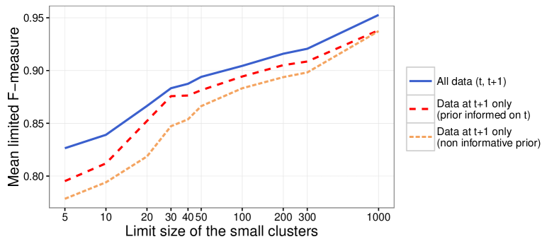
Figure S1: Mean limited $\mathcal{F}$-measure according to the limit size of rare populations, over 300 simulations

D flowMeans applied to the DALIA-1 trial

Here we provide additional representation of the results from flowMeans applied to the DALIA-1 trial and compared to NPflow for the effector CD4+ T-cell population. Overall the results of flowMeans are comparable to those of NPflow without the sequential posterior approximation strategy, as can be seen from Figures S2, S3 and S4, while the sequential strategy outperforms both.

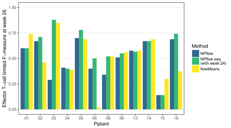
Figure S2: Limited $\mathcal{F}$-measures for the effector T-cell population from the DALIA-1 trial two weeks after HAART interruption for NPflow with or without the sequential strategy and for flowMeans, compared to manual gating.

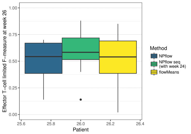
Figure S3: Boxplots of the limited $\mathcal{F}$-measures for the effector CD4+ T-cell population from the DALIA-1 trial two weeks after HAART interruption for NPflow with or without the sequential strategy and for flowMeans, compared to manual gating.

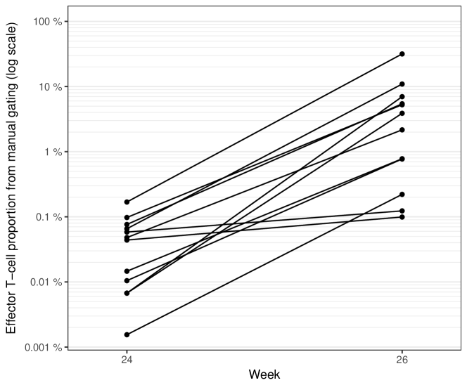
Figure S4: Paired proportions of effector CD4+ T-cells in the DALIA-1 trial before and after HAART interruption from manual gating.

References

• Aghaeepour et al. (2013) Aghaeepour, N., Finak, G., Hoos, H., Mosmann, T. R., Brinkman, R. R., Gottardo, R., and Scheuermann, R. H. (2013). Critical assessment of automated flow cytometry data analysis techniques. Nature methods 10, 228–238.
• Aghaeepour et al. (2011) Aghaeepour, N., Nikolic, R., Hoos, H. H., and Brinkman, R. R. (2011). Rapid cell population identification in flow cytometry data. Cytometry. Part A : the journal of the International Society for Analytical Cytology 79, 6–13.
• Azzalini and Capitanio (2003) Azzalini, A. and Capitanio, A. (2003). Distributions generated by perturbation of symmetry with emphasis on a multivariate skew t-distribution. Journal of the Royal Statistical Society: Series B (Statistical Methodology) 65, 367–389.
• Azzalini and Valle (1996) Azzalini, A. and Valle, A. D. (1996). The multivariate skew-normal distribution. Biometrika 83, 715–726.
• Biernacki et al. (2000) Biernacki, C., Celeux, G., and Govaert, G. (2000). Assessing a mixture model for clustering with the integrated completed likelihood. IEEE transactions on pattern analysis and machine intelligence 22, 719–725.
• Binder (1978) Binder, D. A. (1978). Bayesian Cluster Analysis. Biometrika 65, 31–38.
• Binder (1981) Binder, D. A. (1981). Approximations to Bayesian Clustering Rules. Biometrika 68, 275–285.
• Brinkman et al. (2007) Brinkman, R. R., Gasparetto, M., Lee, S.-J. J., Ribickas, A. J., Perkins, J., Janssen, W., Smiley, R., and Smith, C. (2007). High-content flow cytometry and temporal data analysis for defining a cellular signature of graft-versus-host disease. Biology of blood and marrow transplantation : journal of the American Society for Blood and Marrow Transplantation 13, 691–700.
• Caron et al. (2008) Caron, F., Davy, M., Doucet, A., Duflos, E., and Vanheeghe, P. (2008). Bayesian Inference for Linear Dynamic Models With Dirichlet Process Mixtures. IEEE Transactions on Signal Processing 56, 71–84.
• Caron et al. (2017) Caron, F., Neiswanger, W., Wood, F., Doucet, A., and Davy, M. (2017). Generalized Pólya Urn for Time-Varying Pitman-Yor Processes. Journal of Machine Learning Research 18, 1–32.
• Caron et al. (2014) Caron, F., Teh, Y. W., and Murphy, T. B. (2014). Bayesian nonparametric Plackett–Luce models for the analysis of preferences for college degree programmes. The Annals of Applied Statistics 8, 1145–1181.
• Chan et al. (2008) Chan, C., Feng, F., Ottinger, J., Foster, D., West, M., and Kepler, T. B. (2008). Statistical mixture modeling for cell subtype identification in flow cytometry. Cytometry. Part A : the journal of the International Society for Analytical Cytology 73, 693–701.
• Cron et al. (2013) Cron, A., Gouttefangeas, C., Frelinger, J., Lin, L., Singh, S. K., Britten, C. M., Welters, M. J. P., van der Burg, S. H., West, M., and Chan, C. (2013). Hierarchical modeling for rare event detection and cell subset alignment across flow cytometry samples. PLoS computational biology 9, e1003130.
• Dahl (2006) Dahl, D. B. (2006). Model-Based Clustering for Expression Data via a Dirichlet Process Mixture Model. In Do, K.-A., Müller, P., and Vannucci, M., editors, Bayesian Inference for Gene Expression and Proteomics, chapter 10, pages 201–218. Cambridge University Press, Cambridge.
• Dundar et al. (2014) Dundar, M., Akova, F., Yerebakan, H. Z., and Rajwa, B. (2014). A non-parametric Bayesian model for joint cell clustering and cluster matching: identification of anomalous sample phenotypes with random effects. BMC Bioinformatics 15, 314.
• Escobar and West (1995) Escobar, M. D. and West, M. (1995). Bayesian Density Estimation and Inference Using Mixtures. Journal of the American Statistical Association 90, 577–588.
• Ferguson (1973) Ferguson, T. S. (1973). A Bayesian analysis of some nonparametric problems. The Annals of Statistics 1, 209–230.
• Finak et al. (2009) Finak, G., Bashashati, A., Brinkman, R., and Gottardo, R. (2009). Merging mixture components for cell population identification in flow cytometry. Advances in bioinformatics 2009, 247646.
• Finak et al. (2010) Finak, G., Perez, J.-M., Weng, A., and Gottardo, R. (2010). Optimizing transformations for automated, high throughput analysis of flow cytometry data. BMC Bioinformatics 11, 546.
• Fraley and Raftery (2007) Fraley, C. and Raftery, A. E. (2007). Bayesian Regularization for Normal Mixture Estimation and Model-Based Clustering. Journal of Classification 24, 155–181.
• Fritsch and Ickstadt (2009) Fritsch, A. and Ickstadt, K. (2009). Improved criteria for clustering based on the posterior similarity matrix. Bayesian Analysis 4, 367–392.