Hybrid control trajectory optimization under uncertainty

Abstract

Trajectory optimization is a fundamental problem in robotics. While optimization of continuous control trajectories is well developed, many applications require both discrete and continuous, i.e. hybrid controls. Finding an optimal sequence of hybrid controls is challenging due to the exponential explosion of discrete control combinations. Our method, based on Differential Dynamic Programming (DDP), circumvents this problem by incorporating discrete actions inside DDP: we first optimize continuous mixtures of discrete actions, and, subsequently force the mixtures into fully discrete actions. Moreover, we show how our approach can be extended to partially observable Markov decision processes (POMDPs) for trajectory planning under uncertainty. We validate the approach in a car driving problem where the robot has to switch discrete gears and in a box pushing application where the robot can switch the side of the box to push. The pose and the friction parameters of the pushed box are initially unknown and only indirectly observable.

I INTRODUCTION

Many control applications require both discrete and continuous, i.e. hybrid controls. For example, consider a car with continuous acceleration and direction control but discrete gears [1]. Switching gears changes the dynamics of the car. Another example is pushing a box [2, 3, 4] where the agent can select not only a continuous pushing direction and velocity but also a discrete side to push. Hybrid control is important also in other applications, for example, chemical engineering processes involving on-off valves [5].

Hybrid control is an active research topic [6, 7, 8, 9, 10, 1, 11]. In this paper, we investigate systems with non-linear dynamics and long sequences of hybrid controls and states (trajectories). We provide hybrid control trajectory planning methods for optimizing linear feedback controllers in systems with stochastic dynamics and partial observability which is a challenging but common setting in robotic applications.

In the box pushing application that motivated this paper, we investigate the problem of a robot pushing an unknown object to a predefined location.

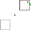
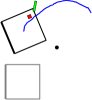
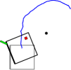
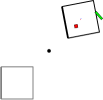
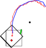
Figure 1: Hybrid control box pushing. The robot tries to push the box with a green finger to the grey target position without hitting the black obstacle in the middle. The robot chooses at each time step a box side to push (discrete action), and a continuous pushing velocity and direction (continuous action). When pushed forward the box also rotates around the red center of friction. Left: The robot observes the box fully and can predict box movement. Right: The robot pushes a partially observed box with stochastic dynamics; the actual red trajectory differs from the expected blue trajectory. Partial observability makes trajectory optimization hard: pushing close to a box corner increases the probability of missing the box. A hybrid approach can directly switch the side to push and avoid considering moving the finger over corners.

Fig. 1 shows examples of pushing trajectories generated by our hybrid control approach. In object pushing, the robot may not know in advance the physical properties of the object such as the friction parameters or the center of friction which is the point around which the object rotates when pushed. The actual center of friction and friction parameters may vary considerably between different objects. Moreover, the robot can only make noisy observations about the current pose of the object, using, for example, a vision sensor. The robot needs to take this observation and dynamics uncertainty into account in order to accomplish its task. For example, when pushing a box to a predefined location, the robot needs to consider how to move its finger along the box edge. However, if the robot is not certain about the actual pose of the box it may miss the box when pushing close to the box corners. This may make approaches with continuous control, such as differential dynamic programming (DDP) reluctant to consider moving the finger around box corners and converge to local optima as shown experimentally in Section VI. A hybrid approach can directly switch the side of the box to push and succeed under uncertainty.

For modeling trajectory optimization under both uncertain dynamics and sensing we use a partially observable Markov decision process (POMDP), and, model uncertain box pushing parameters as part of the POMDP state space. Moreover, control limits are common in robotics; for example, joint motors have physical limits. In the pushing application, the pushing velocity and direction are limited. We show how to add hard limits to DDP based POMDP trajectory optimization, which has so far only been shown for deterministic MDPs [12]. Below, we summarize the major contributions of this paper:

• Hybrid Trajectory Optimization: We introduce trajectory optimization with discrete and continuous actions using differential dynamic programming (DDP).

• Extension to Partially Observable Environments: We introduce the first POMDP trajectory optimization algorithm with hybrid controls.

• Hard Control Limits: Inspired by hard-control limits for trajectory optimization [12], we introduce hard control limits for POMDP trajectory optimization.

• Box-Pushing Application: We use for the first time a POMDP formulation for pushing an unknown object in a task specific way. Taking uncertainty into account is required for performing the task.

II RELATED WORK

In this paper, we consider hybrid control [6, 13, 7, 8, 9, 10, 1, 11] for finite discrete time trajectory optimization [14] in systems with non-linear stochastic dynamics and noisy, partial state information. We optimize time varying linear feedback controllers producing a trajectory consisting of states, covariances, and hybrid controls.

There are many methods for optimizing continuous control trajectories [14, 15, 16, 17]. Discrete controls present a challenge due to the exponential number of discrete control combinations w.r.t. the planning horizon. The naive approach of optimizing continuous controls for each combination of discrete controls scales only to a few time steps. [18] uses a tree of linear quadratic regulator (LQR) solutions for discrete action combinations and introduces a technique for pruning the tree but the tree may still grow exponentially over time.

[11] tries to find a local optimum by performing continuous control optimization and local discrete control improvements iteratively. Hybrid control problems can be also translated into mixed integer non-linear programming (MINLP) problems. However, in complex problems, hybrid control MINLP solutions can be restricted to only a few time step horizons [9]. [1] shows how to apply “convexification”, introduced in [8], for discrete MINLP variables in fully observable deterministic dynamic problems. “Convexification” transforms discrete controls into weights replacing the original dynamics function with a convex mixture. We show how to apply a similar idea to differential dynamic programming (DDP) with stochastic dynamics and partial observations. Instead of using hybrid control for optimizing trajectories, reinforcement learning approaches based on the options framework can compute high level discrete actions, also called options [19], and execute a continuous control policy for each high level action.

RRTs. Rapidly-exploring random trees (RRTs) [20] are often used for trajectory initialization. [21] uses RRTs in hybrid control trajectory planning of fully observable systems. [22] uses also hybrid, that is, discrete and continuous actions, for pushing objects from an initial three dimensional configuration into another final configuration. Contrary to our work, [22] does not do trajectory optimization and does not take uncertainty into account.

POMDPs. Our proposed trajectory optimization approach plans under model, sensing, and actuation uncertainty. [23] and [24] investigate partial observations for computing switching times in switched systems by providing simple analytic examples of a few time steps. However, [23, 24] do not model state uncertainty. Previously, planning under uncertainty has been investigated in simulated robotic tasks in [25, 26, 27]. [27] presents a sampling based POMDP approach for continuous states and actions. [27] uses the POMDP approach for Bayesian reinforcement learning in a simulated pendulum swingup experiment. [28] use feedback based motion-planning with uncertainty and partial observations. [28] target navigation type of applications and use probabilistic roadmap planning to generate a graph where graph nodes represent locations. One classic way of dealing with observation uncertainty is to assume maximum likelihood observations [15]. [17] uses shooting methods for POMDP trajectory optimization. The POMDP approach of [16] is based on iterated linear quadratic Gaussian (iLQG) control with covariance linearization. In this paper, we extend the fully observable iLQG/DDP [12] algorithm as well as the iLQG/DDP based POMDP approach of [16] to hybrid controls. We also show a straightforward way of using hard control limits with iLQG/DDP based POMDP.

Box pushing. When pushing an unknown object a robot needs to plan its motions and pushing actions while taking model [29], sensing, and actuation uncertainty into account. Therefore, we model the pushing task as a hybrid control continuous state POMDP. We base our box pushing simulation on the same quasi-static physics model [30] utilized in [2, 3, 4]. [30] shows how to find out friction parameters but not how to plan for a specific task. [31] discretizes the state space potentially increasing the state space size exponentially w.r.t. the number of dimensions (also known as the state-space explosion problem). Instead of prespecified pushing motions, our approach could be used for planning pushing trajectories in the higher level task planning approach of [2, 3] to handle partly known objects or a specific task.

III PRELIMINARIES

In this section, we first define the problem and subsequently discuss differential dynamic programming, which we extend to hybrid control in the following sections.

Figure 2: Graphical illustration of hybrid sequential control. At time step $t$ the agent executes continuous and discrete controls $\boldsymbol{u}_{t}$ and $a_{t}$, pays a cost $c_{t}(\boldsymbol{x}_{t},\boldsymbol{u}_{t},a_{t})$, and the state changes from $\boldsymbol{x}_{t}$ to $\boldsymbol{x}_{t+1}$. Under partial observability the agent does not see $\boldsymbol{x}_{t}$ but instead makes an observation $\boldsymbol{z}_{t}$. The goal is to minimize the total cost over a finite number of time steps.

III-A Problem statement

In finite time-discrete hybrid sequential control, at each time step $t$, the agent executes continuous control $\boldsymbol{u}_{t}$ and discrete control $a_{t}$ out of $N_{a}$ possibilities, incurs a cost of the form $c_{t}(\boldsymbol{x}_{t},\boldsymbol{u}_{t},a_{t})$ for intermediate time steps and traditionally $c_{T}(\boldsymbol{x}_{t})$ for the final time step $T$. Subsequently, the world changes from state $\boldsymbol{x}_{t}$ to state $\boldsymbol{x}_{t+1}$ according to a dynamics function $\boldsymbol{x}_{t+1}=\boldsymbol{f}(\boldsymbol{x}_{t},\boldsymbol{u}_{t},a_{t})$. The goal is to minimize the total cost $c(\boldsymbol{x}_{T})+\sum_{t=0}^{T-1}c(\boldsymbol{x}_{t},\boldsymbol{u}_{t},a_{t})$. Fig. 2 illustrates this process.

In a partially observable Markov decision process (POMDP), the agent does not directly observe the system state but instead makes an observation $\boldsymbol{z}_{t}$ at each time step $t$. In a POMDP, state dynamics and the observation function are stochastic. While the agent does not observe the current state directly, the agent can choose the control based on the belief $P(\boldsymbol{x}_{t})$, a probability distribution over states, which summarizes past controls and observations and is a sufficient statistic for optimal decision making.

Because solving POMDPs exactly is intractable even for small discrete problems, Gaussian belief space planning methods [16, 32, 17] assume a multi-variate Gaussian distribution for the state space, transitions, and observations with a Gaussian initial belief distribution $\boldsymbol{x}_{0}\sim\mathcal{N}(\hat{\boldsymbol{x}}_{0},\boldsymbol{\Sigma}_{0})$. We denote with $\hat{\boldsymbol{x}}$ the mean and with $\boldsymbol{\Sigma}$ the covariance of the belief. In a hybrid control Gaussian POMDP, the next state depends on a possibly non-linear function $\boldsymbol{f}(\boldsymbol{x}_{t},\boldsymbol{u}_{t},a_{t})$:

$$\boldsymbol{x}_{t+1}=\boldsymbol{f}(\boldsymbol{x}_{t},\boldsymbol{u}_{t},a_{t})+\boldsymbol{m}\;,$$ (1)

where $\boldsymbol{m}\sim\mathcal{N}(0,M(\boldsymbol{x},\boldsymbol{u},a))$ is state and control specific multi-variate Gaussian noise. The observation $\boldsymbol{z}_{t}$ at each time step is specified by a possibly non-linear function $\boldsymbol{h}(\boldsymbol{x}_{t})$ with additive Gaussian noise:

$$\boldsymbol{z}_{t}=\boldsymbol{h}(\boldsymbol{x}_{t})+\boldsymbol{n}\;,$$ (2)

where $\boldsymbol{n}\sim\mathcal{N}(0,N(\boldsymbol{x}))$ is state specific multi-variate Gaussian noise.

The immediate cost function is of the form $c(\boldsymbol{x},\boldsymbol{u},a,\boldsymbol{\Sigma})$ for intermediate time steps and $c(\boldsymbol{x})$ for the final time step. Many methods use the covariance as a term in their cost function to penalize high uncertainty in state estimates.

III-B Differential dynamic programming

DDP [33] is a widely used method for trajectory optimization with fast convergence [34, 35] and the ability to generate feedback controllers. In this section, we discuss DDP and iterative linear quadratic Gaussian (iLQG) [36], a special version of DDP which disregards second order dynamics derivatives and adds regularization and line search to deal with non-linear dynamics.

We will describe DDP here briefly. Please, see [12] for a more detailed description. DDP optimization starts from an initial nominal trajectory, a sequence of controls and states and then applies back and forward passes in succession. In the backwards pass, DDP quadratizes the value function around the nominal trajectory and uses dynamic programming to compute linear forward and feedback gains at each time step. In the forward pass, DDP uses the new policy to project a new trajectory of states and controls. The new trajectory is then used as nominal trajectory in the next backwards pass and so on. A short description follows but please see [33, 36, 12] for more details.

Denote the nominal trajectory with upper bars and the differences between the state and control w.r.t. the nominal trajectory as $\Delta\boldsymbol{x}=\boldsymbol{x}-\boldsymbol{\bar{x}}$ and $\Delta\boldsymbol{u}=\boldsymbol{u}-\boldsymbol{\bar{u}}$, respectively. DDP assumes that the value function at time step $t$ is of quadratic form

$$V_{t}(\boldsymbol{x})=V+\Delta\boldsymbol{x}^{T}\boldsymbol{V}_{\boldsymbol{x}}+\Delta\boldsymbol{x}^{T}\boldsymbol{V}_{\boldsymbol{x}\boldsymbol{x}}\Delta\boldsymbol{x}.,$$ (3)

The one time step value difference between time step $t$ and $t+1$ w.r.t. states and controls

$$Q_{t}(\Delta\boldsymbol{x},\Delta\boldsymbol{u})=c_{t}(\boldsymbol{x}+\Delta\boldsymbol{x},\boldsymbol{u}+\Delta\boldsymbol{u})-c_{t}(\boldsymbol{x},\boldsymbol{u})+$$

$$V_{t+1}(\boldsymbol{f}(\boldsymbol{x}+\Delta\boldsymbol{x},\boldsymbol{u}+\Delta\boldsymbol{u}))-V_{t+1}(\boldsymbol{f}(\boldsymbol{x},\boldsymbol{u}))$$

is also assumed quadratic.

Given $V_{t+1}(\boldsymbol{x})$ we can compute the continuous control $\boldsymbol{u}$ at time step $t$:

$$\boldsymbol{u} =\boldsymbol{K}(\Delta\boldsymbol{x})+\boldsymbol{k}+\boldsymbol{\bar{u}}$$ (4)

$$\boldsymbol{K} =-\boldsymbol{Q}_{\boldsymbol{u}\boldsymbol{u}}^{-1}\boldsymbol{Q}_{\boldsymbol{u}\boldsymbol{x}}\;\;\;\;\textrm{and}\;\;\;\;\boldsymbol{k}=-\boldsymbol{Q}_{\boldsymbol{u}\boldsymbol{u}}^{-1}\boldsymbol{Q}_{\boldsymbol{u}}\;.$$ (5)

where $\boldsymbol{K}$ is the feedback gain and $\boldsymbol{k}$ the forward gain of the linear feedback controller. $\boldsymbol{Q}_{\boldsymbol{u}\boldsymbol{u}}$, $\boldsymbol{Q}_{\boldsymbol{u}\boldsymbol{x}}$, and $\boldsymbol{Q}_{\boldsymbol{u}}$ are computed based on $Q_{t}(\Delta\boldsymbol{x},\Delta\boldsymbol{u})$ as detailed in [12].

Recently, [12] introduced a version of DDP that allows efficient computation with hard control limits. Hard control limits require quadratic programming (QP) for computing the forward gains $\boldsymbol{k}$:

$$\boldsymbol{k}=\arg\min_{\Delta\boldsymbol{u}}\frac{1}{2}\Delta\boldsymbol{u}^{T}\boldsymbol{Q}_{\boldsymbol{u}\boldsymbol{u}}\Delta\boldsymbol{u}+\Delta\boldsymbol{u}^{T}\boldsymbol{Q}_{\boldsymbol{u}}$$

$$\boldsymbol{u}_{\textrm{LB}}\leq\boldsymbol{u}+\Delta\boldsymbol{u}\leq\boldsymbol{u}_{\textrm{UB}}\;,$$ (6)

where $\boldsymbol{u}_{\textrm{LB}}$ and $\boldsymbol{u}_{\textrm{UB}}$ are the lower and upper limits, respectively. For the feedback gain matrix $\boldsymbol{K}$, the rows corresponding to clamped controls are set to zero. To solve QPs, [12] provides a gradient descent algorithm which allows initialization of the QP with a previously computed forward gain. Good initialization makes the approach computationally efficient. In the next Section, we will discuss how to extend the QP approach with equality constraints which allows action probabilities needed by our hybrid control approach.

IV HYBRID TRAJECTORY OPTIMIZATION

The first problem with hybrid control is that the discrete action choice depends on the combination of discrete actions at all time steps resulting in exponentially many combinations. The second problem is that in non-linear problems we can adjust the approximation error due to linearization for continuous but not for discrete controls. For example, continuous iLQG adjusts the linearization error by scaling the forward gain $\boldsymbol{k}$ with a real valued parameter $\alpha$ during the forward pass (when $\alpha$ approaches zero the linearization error approaches zero). However, for discrete actions, decreasing the amount of control change is not straightforward.

Below, we present three approaches for optimizing hybrid control DDP policies. The first two are simple greedy baseline approaches which we provide for comparison. The third more powerful approach uses a continuous mixture of discrete actions driving the mixture during optimization into single selection using a special cost function.

IV-A Greedy discrete action choice

During the DDP back pass, at each time step, the greedy approach computes the expected value at the nominal state and control for each discrete action separately and selects the action which yields minimum expected cost. In the greedy approach, there is no feedback control for discrete actions, only the fixed actions computed during the DDP back pass.

IV-B Interpolated discrete action choice

The second baseline approach for hybrid control attempts to smoothly scale the linearization error w.r.t. discrete controls. The approach interpolates between nominal and new optimized discrete actions. First, the interpolated approach computes new actions identically to the greedy approach, but, then uses only a fraction $\alpha$ of the new discrete actions which differ from the old nominal actions. The selection of actions is done evenly over the time steps. For example, for $\alpha=0.5$ every other new discrete control would be used.

IV-C Mixture of discrete actions

The approach that we propose for hybrid control uses a mixture of discrete actions assigning a continuous pseudo-probability to each discrete action. During optimization, using a specialized cost function which is discussed further down, we drive the mixture to select a single discrete action.

Our modified control $\hat{\boldsymbol{u}}$ is

$$\hat{\boldsymbol{u}}=\begin{bmatrix}\boldsymbol{u}\\ \boldsymbol{p_{a}}\end{bmatrix}\;,$$ (7)

where $\boldsymbol{p_{a}}$ contains the action probabilities. The dimensionality of the controls increases by the number of discrete actions. For simplicity, we assume here a single discrete control variable but our approach directly extends to several discrete control variables. For several discrete controls, the dimensionality would either be the sum of discrete control dimensions if one treats discrete controls as independent, or, the product of discrete control dimensions if one wants better accuracy.

For hybrid controls, the dynamics model $\boldsymbol{f}(\boldsymbol{x},\boldsymbol{u},a)$ depends on both continuous controls $\boldsymbol{u}$ and discrete actions $a$. The new dynamics model is a mixture of the original one:

$$\hat{\boldsymbol{f}}(\boldsymbol{x},\hat{\boldsymbol{u}})=\sum_{a}p_{a}\boldsymbol{f}(\boldsymbol{x},\boldsymbol{u},a)\;.$$ (8)

Note that (8) is essentially identical to the “convexified” dynamics function in [8] for fully observable MINLP hybrid control. However, [8] does not present a mixture model for immediate cost functions and our special cost function further down that forces the system into a bang-bang solution differs from the one in [8] because of the positive-definite Hessian for cost functions in DDP.

For hybrid controls, we define the cost function $c(\boldsymbol{x},\boldsymbol{u},a)$ in the mixture model as

$$\hat{c}(\boldsymbol{x},\hat{\boldsymbol{u}})=\sum_{a}\phi(p_{a})c(\boldsymbol{x},\boldsymbol{u},a)\;,$$ (9)

where $\phi(\cdot)$ is a smoothing function to make the Hessian of the cost function positive-definite w.r.t. the linear parameters $p_{a}$. In the experiments, we used a pseudo-Huber smoothing function

$$\phi(p)=\phi(p,0.01),\phi(p,k)=\sqrt{p^{2}+k^{2}}-k$$ (10)

which is close to linear but has a positive second derivative.

To optimize the forward and feedback gains during dynamic programming, we add the following inequality and equality constraints for the probabilities to the quadratic program in Equation (6):

$$\boldsymbol{0}\leq\boldsymbol{p}\leq\boldsymbol{1}\;,\;\;\sum_{a}p_{a}=1\;.$$ (11)

We extend the efficient gradient descent method for quadratic programming from [12] to deal with the equality constraint (11). Shortly: 1) we subtract the mean from the search direction of probabilities satisfying the equality constraint, 2) we modify the Armijo line search step size dynamically so that we do not overstep probability inequality constraints.

$\hat{\boldsymbol{f}}(\boldsymbol{x},\boldsymbol{u},\boldsymbol{p})$ can be seen as the expected dynamics of a partially stochastic policy. For such expected dynamics there may not be any actual control values that would result in such dynamics. For example, in the box pushing application a mixture of discrete actions could correspond to pushing with several fingers although the robot may only have one finger. However, allowing for stochastic discrete actions in the beginning of optimization allows convergence to a good solution, even if we force the actions to become deterministic later. Our optimization procedure takes care of the major problems with sequential decision making with hybrid controls: the procedure allows to continuously decrease the approximation error due to linearization making local updates possible but is not subject to the combinatorial explosion of discrete action combinations. Next we discuss how to force a deterministic policy for discrete actions.

Forcing deterministic discrete actions. In the end, we want a valid deterministic policy for discrete actions. Therefore, we explicitly assign a cost to stochastic discrete actions that increases during optimization driving stochastic discrete controls into deterministic ones. Entropy would be a natural, widely used, cost measure. However, the Hessian matrix of an entropy based cost function is not positive-definite (the second derivative is always negative). Instead, we use the following similarly shaped smoothed piece-wise cost function on stochastic discrete actions

$$c_{\textrm{ST}}(\boldsymbol{x},\boldsymbol{u},\boldsymbol{p})=C_{\textrm{ST}}\sum_{a}\begin{dcases}\phi(p_{a})&\text{if }p_{a}<p_{\textrm{th}}\\ \phi\left(\frac{(1-p_{a})}{p_{\textrm{th}}/(1-p_{\textrm{th}})}\right)&\text{if }p_{a}\geq p_{\textrm{th}}\\ \end{dcases}\;,$$ (12)

where $p_{\textrm{th}}=1/N_{a}$ and $C_{\textrm{ST}}$ is an adaptive constant. Note that while $c_{\textrm{ST}}(\boldsymbol{x},\boldsymbol{u},\boldsymbol{p})$ is discontinuous at $p_{\textrm{th}}$, derivatives can be computed below and above $p_{\textrm{th}}$ and the cost drives solutions away from $p_{\textrm{th}}$ for increasing $C_{\textrm{ST}}$. When at $p_{\textrm{th}}$, which corresponds to a uniform distribution, the cost achieves its maximum. Note that any cost measure with zero cost for probabilities $0$ and $1$ is bound to have a discontinuity when the second derivative has to be positive. Intuitively, the positive second derivative forces the graph of the cost measure to always curve upwards resulting in a discontinuity at the point where the graph starting from $0$ meets the graph ending at $1$.

Tiny image on the right shows the cost function (solid) and its second derivative (dashed) for two discrete states and $C_{\textrm{ST}}=1$. The x-axis shows the state probability.

Practicalities. During optimization we double $C_{\textrm{ST}}$ everytime the cost decrease between DDP iterations is below a threshold. We set $C_{\textrm{ST}}$ to a maximum value when half of the maximum number of iterations has elapsed. This allows for both smoothly increasing determinicity of discrete actions and then finally deterministic action selection. Since we run the algorithm for a finite number of iterations and do not increase $C_{\textrm{ST}}$ to infinity some tiny stochasticity may remain. Therefore, we select the most likely discrete action during evaluation. Note also that due to the linear feedback control affecting probabilities we normalize probabilities during the forward pass.

V HYBRID TRAJECTORY OPTIMIZATION FOR POMDPS

We are now ready to discuss hybrid control of POMDP trajectories. We start with an iLQG approach for POMDPs [16] and then discuss how the iLQG POMDP can be extended with hybrid controls and hard control limits.

V-A DDP for POMDP trajectory optimization

The iLQG POMDP approach of [16] extends iLQG [12] to POMDPs by using a Gaussian belief $\mathcal{N}(\hat{\boldsymbol{x}},\boldsymbol{\Sigma})$, instead of the fully observable state $\boldsymbol{x}$. In the forward pass iLQG POMDP uses a standard extended Kalman filter (EKF) to compute the next time step belief. For the backward pass, iLQG POMDP linearizes the covariance in addition to quadratizing states and controls. The value function in Equation (3) becomes

$$V_{t}(\hat{\boldsymbol{x}},\boldsymbol{\Sigma})=V+\Delta\hat{\boldsymbol{x}}^{T}\boldsymbol{V}_{\hat{\boldsymbol{x}}}+\Delta\hat{\boldsymbol{x}}^{T}\boldsymbol{V}_{\hat{\boldsymbol{x}}\hat{\boldsymbol{x}}}\Delta\hat{\boldsymbol{x}}+\boldsymbol{V}^{T}_{\boldsymbol{\Sigma}}\textrm{vec}[\Delta\boldsymbol{\Sigma}],$$ (13)

where $\textrm{vec}[\Delta\boldsymbol{\Sigma}]$ is the difference between the current and nominal covariance stacked column-wise into a vector and $\boldsymbol{V}^{T}_{\boldsymbol{\Sigma}}$ is a new linear value function parameter. The related control law/policy is shown in [16, Equation (23)].

V-B Hybrid control for POMDP trajectory optimization

In the partially observable case, the direct and indirect cost of uncertainty propagates through $\boldsymbol{V}_{\boldsymbol{\Sigma}}$ into other value function components and the optimal policy has to take uncertainty into account. However, the control law in [16, Equation (23)] in iLQG POMDP is of equal form to the one in basic iLQG shown in Equation (5). The only difference is that $\boldsymbol{Q}_{\boldsymbol{u}\boldsymbol{u}}$, $\boldsymbol{Q}_{\boldsymbol{u}\boldsymbol{x}}$, and $\boldsymbol{Q}_{\boldsymbol{u}}$ shown in Equation (5) are influenced by $\boldsymbol{V}_{\boldsymbol{\Sigma}}$ from future time steps [16]. This means that we can directly optimize controls using the quadratic program (QP) shown in Equation (6). Therefore, we can use hard limits and equality constraints on continuous controls in iLQG POMDP which is one technical insight in this paper.

A question this raises is whether we can also apply our proposed hybrid control approach to iLQG POMDP? Yes. Since our method of discrete action mixtures described in Section IV-C hides the action mixture inside the dynamics and cost functions, and, since the observation function does not directly depend on the controls, we can directly use the proposed hybrid control approach for POMDP optimization.

VI EXPERIMENTS

We experimentally validate our hybrid control approach “Mixture”, described in Section IV-C, in two different simulations: autonomous car driving and pushing of an unknown box. We are not aware of previous algorithms for trajectory planning under uncertainty which operate directly on both continuous and discrete actions. However, in the car driving and box pushing applications, we can reasonably map the hybrid controls directly to continuous controls and compare against continuous iLQG [12] and continuous iLQG POMDP [16], extended to support hard control limits, as described in Section V-B. Note that in many hybrid control applications, for example, with discrete switches or on-off valves, mapping hybrid controls to continuous ones may not be possible and a hybrid approach is required. We also compare with greedy action selection “Greedy” described in Section IV-A, and interpolated greedy action selection “Interpolate” described in Section IV-B. We used a time horizon of $T=500$ and ran up to $400$ optimization iterations for each method. We set the maximum for $C_{\textrm{ST}}$ (please, see Section IV-C) to $1.28$. $C_{\textrm{ST}}$ starts from zero, increases to $0.01$, and then doubles every time the cost difference is below $0.01$ in box pushing and $0.0001$ in car driving.

VI-A Autonomous car driving

In autonomous car driving, the robot drives a nonholonomic car, switches discrete gears, accelerates, and tries to steer the car to zero position and pose. The dynamics are identical to the car parking dynamics in [12] with a few differences. The system state $\boldsymbol{x}=(x,y,w,v_{\textrm{CAR}})$ consists of the position of the car $(x,y)$, the car angle $w$, and the car velocity $v_{\textrm{CAR}}$. The continuous controls $\boldsymbol{u}=(w_{\textrm{WHEEL}},acc_{\textrm{CAR}})$ select the front wheel angle $w_{\textrm{WHEEL}}\in[-0.5,0.5]$ and car acceleration $acc_{\textrm{CAR}}\in[0,0.5]$. We have three discrete actions: the robot can select either 1st or 2nd gear, or alternatively break.

In 2nd gear acceleration is halved and for breaking acceleration is negative. The break, 1st and 2nd gear have a soft velocity limit: for the break and 2nd gear, when $v_{\textrm{CAR}}>4$, and for the 1st gear when $v_{\textrm{CAR}}>1$, the car is assigned a negative acceleration of $acc_{\textrm{CAR}}=-0.1$ simulating real world engine breaking. Since the 1st gear has a lower soft velocity limit than the 2nd gear but higher acceleration, to achieve high speeds quickly one needs to accelerate first with the 1st gear and then switch to the 2nd gear.

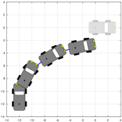
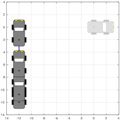
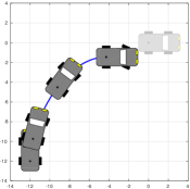
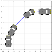
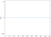
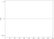
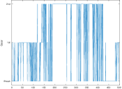
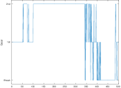
(a) iLQG	(b) Greedy	(c) Interpolate	(d) Mixture

Figure 4: Deterministic autonomous car experiment. The goal is to drive the car quickly to zero position. The top row shows, for each method, the optimized trajectories and the bottom row whether the car breaks, uses the 1st gear, or uses the 2nd gear at each time step.

For initial controls we used $w_{\textrm{WHEEL}}=0$, 1st gear, $acc_{\textrm{CAR}}=0.1$. Non-optimized code on an Intel i7 CPU took $0.47$, $0.88$, $0.93$, and $1.03$ seconds per iteration for the “iLQG”, “Greedy”, “Interpolate”, and “Mixture” methods, respectively. Fig. 3 displays the costs and Fig. 4 shows the resulting trajectories and discrete controls. Due to discontinuities, continuous iLQG has difficulty switching from 1st to 2nd gear and can not achieve maximum velocity. Since policy improvement starts in DDP from the last time step and proceeds to the first, greedy iLQG “Greedy” does not switch to 2nd gear. The low cost policy of the proposed hybrid mixture method “Mixture” utilizes the 1st gear for fast acceleration, the 2nd gear for high velocity, and the break for slowing down. To discourage fast switching one could add a gear/break switching cost.

In addition, we started continuous iLQG from the 2nd gear. Note that in practice starting from 2nd gear can yield high clutch wear. “iLQG” improved from $9.05$ to $6.96$ total cost while “Mixture” was still better with $6.34$ when starting from the 1st gear, due to “iLQG” relying only on the 2nd gear for acceleration instead of strong 1st gear initial acceleration.

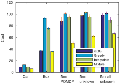
Figure 3: Mean costs and standard errors of the mean for the comparison methods. The deterministic “Car” problem has a single trajectory and thus no standard error. “Mixture” performs overall best and is better than continuous “iLQG” in the three stochastic problems.

VI-B Pushing an object

We will now describe the pushing task where the goal is to push an unknown object into a predefined goal-zone.

State. We define the state as

$$\boldsymbol{x}=(\boldsymbol{x}^{C},w,\boldsymbol{x}^{CF},\mu_{c},c)\;,$$ (14)

where $\boldsymbol{x}^{C}=(x^{C},y^{C})$ denotes the center coordinates and $w$ the rotation angle of the object. $\boldsymbol{x}^{CF}=(x^{CF},y^{CF})$ denotes the center of friction (CF) coordinates relative w.r.t. $\boldsymbol{x}^{C}$. $\mu_{c}$ denotes the friction between the end effector and the object and $c$ the distribution friction coefficient between object and supporting surface [30]. We assume that object edge locations w.r.t. $\boldsymbol{x}^{C}$ are fully observable.

Control action. When pushing we keep the speed of the robot hand constant while using sufficient force to move the hand. The discrete control consists of $e$, the discrete edge of the object to push. The continuous control is

$$\boldsymbol{u}=(u^{e},\alpha^{p},v),$$ (15)

where $u^{e}$, $0\leq u^{e}\leq 1$ is the continuous contact point location along the edge, $\alpha^{p}$, $-0.35\pi\leq\alpha_{p}\leq 0.35\pi$ is the pushing angle w.r.t. the normal unit vector at the contact point w.r.t. the edge, and $v$, $0.01\leq v\leq 3$ is finger velocity. It is possible to parameterize $e$ and $u^{e}$ into a single continuous control. We do this for the continuous control version of iLQG. The continuous control version may not be able to jump easily from one discrete edge to another because of the dynamics discontinuity at the corners and because of potentially missing the box when box pose is uncertain. When pushing the box the finger of the robot can slide along the pushed edge. Combining sliding and non-sliding dynamics we get the pushing dynamics as described in [30].

Observations. At each time step the robot makes an observation about the pose of the object. The observation function in Equation 2 is then $\boldsymbol{h}[\boldsymbol{x}_{t}]=(\boldsymbol{x}^{C},w)$.

Cost function. Our cost function penalizes the robot for not pushing the object into the target pose by $20\phi(x^{C})+20\phi(y^{C})+2\phi(w)$; at each time step penalizes the distance from target location by $0.01(\phi(x^{C},0.1)+\phi(y^{C},0.1))$ and controls by $10^{-6}((\alpha^{p})^{2}+v^{2})$; penalizes the robot for final uncertainty by the sum of all state variances; penalizes for getting too close to an obstacle at position $\boldsymbol{x}^{o}$ by $-0.1\log\Phi((\boldsymbol{x}^{o}-\boldsymbol{x}^{C})^{T}(\boldsymbol{x}^{o}-\boldsymbol{x}^{C})-0.5\sqrt{2})$, where $\Phi(\cdot)$ denotes the Gaussian CDF. Finally, to avoid missing the object, we penalize pushing too close to a corner relative to the object rotation variance $\sigma^{2}_{w}$ by $0.1\exp(10(u^{e}-\cos(\min(3\sigma^{2}_{w},0.5\pi))))+0.1\exp(10(1-\cos(\min(3\sigma^{2}_{w},0.5\pi))-u^{e}))$.

In the box pushing experiment, the goal is to push the box to the target location at zero position. Position $(1,1)$ contains a soft obstacle. We initialize controls to push the bottom edge $e=0$ and $u^{e}=0.5$, $\alpha^{p}=0$, $v=1$, and, for “Mixture” $p_{e}=1-10^{-10}$. In the fully observable version the robot’s planned pushing location and angle correspond to the real ones. In the partially observable POMDP problem “Box POMDP” the controls are w.r.t. the planned pose and not the actual pose, and the robot may miss the box resulting in the box not moving. The initial standard deviation (SD) for the xy-coordinates is $0.01$ and for the rotation angle $0.1$. In “Box POMDP”, the friction parameters are known. In the “Box unknown” experiments, the coordinates of the center of friction are unknown and have initially a SD of $0.2$ and in “Box all unknown” also the friction parameters $\mu_{c}$ and $c$ are not known and have initially a SD of $0.2$. At each time step the robot gets a noisy observation about the box position with SD $0.0001$ and angle of the box with SD $0.033$. The SD of dynamics noise for xy-coordinates and rotation is $0.01$. Friction parameters $\mu_{c}$ and $c$ had a mean of $1$.

For evaluation we sampled friction parameters for “Box unknown” and “Box all unknown”. Moreover, in order to test a variety of different centers of friction (CFs) we selected CFs uniformly between the box left bottom coordinates $(0.2,0.2)$ and the top right coordinates $(0.8,0.8)$ corresponding to sampling from a uniform distribution. For the deterministic “Box” we “sampled” 52 different CFs and for each of the stochastic “Box POMDP”, “Box unknown”, and “Box all unknown” problems 12 different CFs. In the stochastic problems we averaged costs for each CF over 20 sampled trajectories.

Fig. 3 shows the cost means and standard errors over the CFs. The “iLQG”, “Greedy”, “Interpolate”, and “Mixture” methods, on the “Box”/“Box POMDP”/“Box unknown”/“Box all unknown” problems took $0.86/3.03/4.32/8.61$, $1.36/3.53/4.55/8.74$, $1.37/3.75/5.28/10.95$, and $1.59/5.80/8.60/18.06$ seconds per iteration, respectively. “Mixture” performs best. As expected higher uncertainties decrease performance of “Mixture”. “Interpolate”, “Greedy”, and “iLQG” seem to have systematic problems in all setups with high uncertainty. The heuristics of “Interpolate” and “Greedy” do not always work and iLQG gets stuck in local optima. Fig. 5 shows high and low cost examples for both the “Box POMDP” and “Box unknown” problems for “iLQG” and our “Mixture” method. In the worst case, iLQG can not escape local optimums: the cost for potentially missing the box prevents switching pushing sides. In the POMDP problem, for a suitable center of friction, iLQG computes a good policy but in the unknown POMDP problem has even in the best case run away trajectories.

iLQG
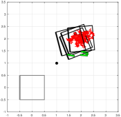
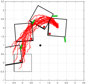
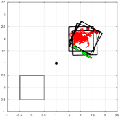
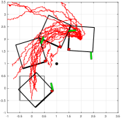
Mixture
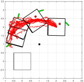
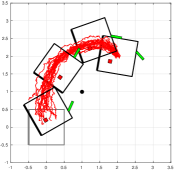
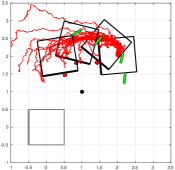
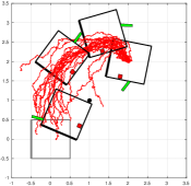
	(a) Worst	(b) Best	(c) Worst	(d) Best
	Box POMDP		Box unknown

Figure 5: Uncertain box pushing. The goal is to push the box using the green finger to zero position while avoiding the obstacle at $(1,1)$. For (a) and (b) the box position and rotation are uncertain and partially observable, but for (c) and (d) also the red center of friction is uncertain. (a) and (c) show worst performance and (b) and (d) the best. For one of the sampled red trajectories ($20$ in each plot) we display four boxes and finger configurations distributed evenly over time. For rotation visualization one box edge is thicker than the others.

VII CONCLUSIONS

We presented a novel DDP approach with linear feedback control for hybrid control of trajectories under uncertainty. The experiments indicate that our approach is useful, especially in POMDP problems. In the future, we plan on applying the approach to a real robot. We may use online replanning to improve the results further.

References

- [1] C. Kirches, S. Sager, H. G. Bock, and J. P. Schlöder, “Time-optimal control of automobile test drives with gear shifts,” Optimal Control Applications and Methods, vol. 31, no. 2, pp. 137–153, 2010.
- [2] M. Dogar and S. Srinivasa, “Push-grasping with dexterous hands: Mechanics and a method,” in Proceedings of the IEEE/RSJ International Conference on Intelligent Robots and Systems (IROS), 2010.
- [3] ——, “A planning framework for non-prehensile manipulation under clutter and uncertainty,” Autonomous Robots, vol. 33, no. 3, pp. 217–236, 2012.
- [4] M. Koval, N. Pollard, and S. Srinivasa, “Pre- and post-contact policy decomposition for planar contact manipulation under uncertainty,” in Proceedings of Robotics: Science and Systems (R:SS), 2014.
- [5] Y. Kawajiri and L. T. Biegler, “Large scale optimization strategies for zone configuration of simulated moving beds,” Computers & Chemical Engineering, vol. 32, no. 1, pp. 135–144, 2008.
- [6] M. S. Branicky, V. S. Borkar, and S. K. Mitter, “A unified framework for hybrid control: Model and optimal control theory,” IEEE Transactions on Automatic Control, vol. 43, no. 1, pp. 31–45, 1998.
- [7] A. Bemporad, G. Ferrari-Trecate, and M. Morari, “Observability and controllability of piecewise affine and hybrid systems,” IEEE Transactions on Automatic Control, vol. 45, no. 10, pp. 1864–1876, 2000.
- [8] S. Sager, Numerical methods for mixed-integer optimal control problems. Der andere Verlag Tönning, Lübeck, Marburg, 2005.
- [9] N. N. Nandola and S. Bhartiya, “A multiple model approach for predictive control of nonlinear hybrid systems,” Journal of process control, vol. 18, no. 2, pp. 131–148, 2008.
- [10] V. Azhmyakov, R. Galvan-Guerra, and M. Egerstedt, “Hybrid lq-optimization using dynamic programming,” in Proceedings of the American Control Conference. IEEE, 2009, pp. 3617–3623.
- [11] F. Zhu and P. J. Antsaklis, “Optimal control of hybrid switched systems: A brief survey,” Discrete Event Dynamic Systems, vol. 25, no. 3, pp. 345–364, 2015.
- [12] Y. Tassa, N. Mansard, and E. Todorov, “Control-limited differential dynamic programming,” in Proceedings of the IEEE International Conference on Robotics and Automation (ICRA). IEEE, 2014, pp. 1168–1175.
- [13] P. Riedinger, F. Kratz, C. Iung, and C. Zanne, “Linear quadratic optimization for hybrid systems,” in IEEE Conference on Decision and Control, vol. 3. IEEE, 1999, pp. 3059–3064.
- [14] O. Von Stryk and R. Bulirsch, “Direct and indirect methods for trajectory optimization,” Annals of operations research, vol. 37, no. 1, pp. 357–373, 1992.
- [15] R. Platt Jr, R. Tedrake, L. Kaelbling, and T. Lozano-Perez, “Belief space planning assuming maximum likelihood observations,” in Robotics: Science and Systems (RSS), 2010.
- [16] J. van den Berg, S. Patil, and R. Alterovitz, “Efficient Approximate Value Iteration for Continuous Gaussian POMDPs,” in Proceedings of the AAAI Conference on Artificial Intelligence. AAAI Press, 2012.
- [17] S. Patil, G. Kahn, M. Laskey, J. Schulman, K. Goldberg, and P. Abbeel, “Scaling up gaussian belief space planning through covariance-free trajectory optimization and automatic differentiation,” in Algorithmic Foundations of Robotics XI. Springer, 2015, pp. 515–533.
- [18] B. Lincoln and B. Bernhardsson, “Lqr optimization of linear system switching,” IEEE Transactions on Automatic Control, vol. 47, no. 10, pp. 1701–1705, 2002.
- [19] C. Daniel, H. van Hoof, J. Peters, and G. Neumann, “Probabilistic inference for determining options in reinforcement learning,” in Proceedings of The European Conference on Machine Learning and Principles and Practice of Knowledge Discovery. Springer, 2016.
- [20] S. LaValle and J. Kuffner, “Rapidly-exploring random trees: Progress and prospects,” Algorithmic and Computational Robotics: New Directions, pp. 293–308, 2001.
- [21] M. S. Branicky and M. M. Curtiss, “Nonlinear and hybrid control via rrts,” in Proc. Intl. Symp. on Mathematical Theory of Networks and Systems, vol. 750, 2002.
- [22] C. Zito, R. Stolkin, M. Kopicki, and J. L. Wyatt, “Two-level RRT planning for robotic push manipulation,” in Proc. of IEEE/RSJ International Conference on Intelligent Robots and Systems (IROS). IEEE, 2012, pp. 678–685.
- [23] M. Egerstedt, S.-i. Azuma, and Y. Wardi, “Optimal timing control of switched linear systems based on partial information,” Nonlinear Analysis: Theory, Methods & Applications, vol. 65, no. 9, pp. 1736–1750, 2006.
- [24] S.-i. Azuma, M. Egerstedt, and Y. Wardi, “Output-based optimal timing control of switched systems,” in International Workshop on Hybrid Systems: Computation and Control. Springer, 2006, pp. 64–78.
- [25] S. Ross, B. Chaib-draa, and J. Pineau, “Bayesian reinforcement learning in continuous POMDPs with application to robot navigation,” in Proceedings of the IEEE International Conference on Robotics and Automation (ICRA). IEEE, 2008, pp. 2845–2851.
- [26] P. Dallaire, C. Besse, S. Ross, and B. Chaib-draa, “Bayesian reinforcement learning in continuous POMDPs with Gaussian Processes,” in Proceedings of the IEEE/RSJ International Conference on Intelligent Robots and Systems (IROS). IEEE, 2009, pp. 2604–2609.
- [27] H. Bai, D. Hsu, and W. S. Lee, “Integrated perception and planning in the continuous space: A POMDP approach,” The International Journal of Robotics Research, vol. 33, no. 9, pp. 1288–1302, 2014.
- [28] A.-A. Agha-Mohammadi, S. Chakravorty, and N. M. Amato, “FIRM: Sampling-based feedback motion planning under motion uncertainty and imperfect measurements,” The International Journal of Robotics Research, vol. 33, no. 2, pp. 268–304, 2014.
- [29] M. Kopicki, S. Zurek, R. Stolkin, T. Moerwald, and J. L. Wyatt, “Learning modular and transferable forward models of the motions of push manipulated objects,” Autonomous Robots, pp. 1–22, 2016.
- [30] K. M. Lynch, H. Maekawa, and K. Tanie, “Manipulation and active sensing by pushing using tactile feedback.” in Proc. of IEEE/RSJ International Conference on Intelligent Robots and Systems (IROS). IEEE, 1992, pp. 416–421.
- [31] M. C. Koval, N. S. Pollard, and S. S. Srinivasa, “Pre-and post-contact policy decomposition for planar contact manipulation under uncertainty,” The International Journal of Robotics Research, vol. 35, no. 1-3, pp. 244–264, 2016.
- [32] D. J. Webb, K. L. Crandall, and J. van den Berg, “Online Parameter Estimation via Real-Time Replanning of Continuous Gaussian POMDPs,” in Proceedings of the IEEE International Conference on Robotics and Automation (ICRA). IEEE, 2014.
- [33] D. Mayne, “A second-order gradient method for determining optimal trajectories of non-linear discrete-time systems,” International Journal of Control, vol. 3, no. 1, pp. 85–95, 1966.
- [34] D. Jacobson and D. Mayne, “Differential dynamic programming,” 1970.
- [35] L.-z. Liao and C. A. Shoemaker, “Advantages of differential dynamic programming over newton’s method for discrete-time optimal control problems,” Cornell University, Tech. Rep., 1992.
- [36] E. Todorov and W. Li, “A generalized iterative lqg method for locally-optimal feedback control of constrained nonlinear stochastic systems,” in Proceedings of the American Control Conference. IEEE, 2005, pp. 300–306.