X-ray and radio observations of the magnetar SGR J1935$+$2154 during its 2014, 2015, and 2016 outbursts

Abstract

We analyzed broad-band X-ray and radio data of the magnetar SGR J1935$+$2154 taken in the aftermath of its 2014, 2015, and 2016 outbursts. The source soft X-ray spectrum $<10$ keV is well described with a BB+PL or 2BB model during all three outbursts. NuSTAR observations revealed a hard X-ray tail, $\Gamma=0.9$, extending up to $79~{}$keV, with flux larger than the one detected $<10$ keV. Imaging analysis of Chandra data did not reveal small-scale extended emission around the source. Following the outbursts, the total $0.5-10$ keV flux from SGR J1935$+$2154 increased in concordance to its bursting activity, with the flux at activation onset increasing by a factor of $\sim 7$ following its strongest June 2016 outburst. A Swift/XRT observation taken $1.5$ days prior to the onset of this outburst showed a flux level consistent with quiescence. We show that the flux increase is due to the PL or hot BB component, which increased by a factor of $25$ compared to quiescence, while the cold BB component $kT=0.47$ keV remained more or less constant. The 2014 and 2015 outbursts decayed quasi-exponentially with time-scales of $\sim 40$ days, while the stronger May and June 2016 outbursts showed a quick short-term decay with time-scales of $\sim 4$ days. Our Arecibo radio observations set the deepest limits on the radio emission from a magnetar, with a maximum flux density limit of $14$ $\mu$Jy for the 4.6 GHz observations and $7$ $\mu$Jy for the 1.4 GHz observations. We discuss these results in the framework of the current magnetar theoretical models.

1 Introduction

A sub-set of isolated neutron stars (NSs), dubbed magnetars, show peculiar rotational properties with low spin periods $P$ in the range of $2-12$ seconds and large spin down rates $\dot{P}$ of the order of $10^{-11}-10^{-12}$ s s^-1. Such properties imply particularly strong surface dipole magnetic fields of the order of $10^{14}-10^{15}$ G. About 24 magnetars with these properties are known in our Galaxy, while one resides in the SMC and another in the LMC. Most magnetars show high X-ray persistent luminosities, often surpassing their rotational energy reservoir, hence, requiring an extra source of power. The latter is believed to be of magnetic origin, associated with their extremely strong outer and/or inner magnetic fields.

Magnetars are among the most variable sources within the NS zoo. Almost all have been observed to emit short ($\sim 0.1$ s), bright ($E_{\rm burst}\approx 10^{37}-10^{41}$ erg), hard X-ray bursts (see Mereghetti et al. 2015; Turolla et al. 2015, for reviews). Such bursting episodes can last days to weeks with varying number of bursts emitted by a given source, ranging from 10s to 100s (e.g., Israel et al. 2008; van der Horst et al. 2012; Lin et al. 2011). These bursting episodes are usually accompanied by changes in the source persistent X-ray emission; an increase by a factor of a few to a $\sim$100 in flux level is usually observed to follow bursting episodes, together with a hardening in the X-ray spectrum (e.g., Kaspi et al. 2014; Ng et al. 2011; Esposito et al. 2011; Coti Zelati et al. 2015). Both properties usually relax quasi-exponentially to pre-burst levels on timescales of weeks to months (Rea & Esposito 2011). Their pulse properties also vary following bursting episodes, with a change in shape and pulse fraction (e.g., Woods et al. 2004; Göǧüş et al. 2002, see Woods & Thompson 2006; Mereghetti 2008 for a review). We note that the magnetar-defining observational characteristics mentioned above have also been observed recently from NS not originally classified as magnetars, i.e., the high-B pulsars PSR J$1846-0258$ (Gavriil et al. 2008) and PSR J$1119-6127$ (Göğüş et al. 2016; Archibald et al. 2016), the central compact object in RCW 103 (Rea et al. 2016), and a low-B candidate magnetar, SGR J$0418+5729$ (Rea et al. 2013). Moreover, a surrounding wind nebula, usually a pulsar associated phenomenon, has now been observed from at least one magnetar, Swift $1834.9-0846$ (Younes et al. 2012, 2016; Granot et al. 2016; Torres 2017).

Magnetars also show bright hard X-ray emission ($>10$ keV) with total energy occasionally exceeding that of their soft X-ray emission. This hard emission is non-thermal in origin, phenomenologically described as a power-law (PL) with a photon index ranging from $\Gamma\sim 1-2$ (see e.g., Kuiper et al. 2006). The hard and soft component properties may also differ (e.g., An et al. 2013; Vogel et al. 2014; Tendulkar et al. 2015). In the context of the magnetar model, the hard X-ray emission has been explained as resonant Compton scattering of the soft (surface) emission by plasma in the magnetosphere (Baring & Harding 2007; Fernández & Thompson 2007; Beloborodov 2013).

So far, only four magnetars have been detected at radio frequencies, excluding the high-B pulsar PSR J$1119-6127$ that exhibited magnetar-like activity (Weltevrede et al. 2011; Antonopoulou et al. 2015; Göğüş et al. 2016; Archibald et al. 2016). The radio emission from the four typical magnetars showed transient behavior, correlated with the X-ray outburst onset (Camilo et al. 2006, 2007; Levin et al. 2010). Rea et al. (2012) showed that all radio magnetars have $L_{\rm X}/\dot{E}<1$ during quiescence. However, the physical mechanism for the radio emission in magnetars (as well as why it has only been detected in a very small number of sources) remains largely unclear (e.g., Szary et al. 2015), and could be inhibited if optimal conditions for the production of pairs are not present (e.g., Baring & Harding 1998).

SGR J$1935+2154$ is a recent addition to the magnetar family, discovered with the Swift/X-Ray Telescope (XRT) on 2014 July 05 (Stamatikos et al. 2014). Subsequent Swift, Chandra and XMM-Newton observations taken in 2014 confirmed the source as a magnetar with a spin period $P=3.25$ s and $\dot{P}=1.43\times 10^{-11}$ s s^-1, implying a surface dipole B-field of $B=2.2\times 10^{14}$ G (Israel et al. 2016b). SGR J1935$+$2154 has been quite active since its discovery with at least 3 other outbursts; 2015 February 22, 2016 May 14, and 2016 June 18. The source is close to the geometrical center of the supernova remnant (SNR) G$57.2+0.8$ at a distance of $\sim 9$ kpc (Pavlović et al. 2013; Sun et al. 2011).

In this paper, we report on the analysis of all X-ray observations of SGR J1935$+$2154 taken after 2014 May, including a NuSTAR observation made within days of the 2015 outburst identifying the broad-band X-ray spectrum of the source. We also report on the analysis of radio observations taken with Arecibo following the 2014 and 2016 June outbursts. X-ray and radio observations and data reduction are reported in Section 2, and analysis results are shown in Section 3. Section 4 discusses the results in the context of the magnetar model, while Section 5 summarizes our findings.

2 Observations and data reduction

2.1 Chandra

Chandra observed SGR J1935$+$2154 three times during its 2014 outburst, and once during its 2016 June outburst. Two of the 2014 observations were in Continuous-Clocking (CC) mode while the other two were taken in TE mode with 1/8th sub-array. We analyzed these observations using CIAO 4.8.2, and calibration files CLADB version 4.7.2.

For the TE mode observations, we extracted source events from a circle with radius 2^′′, while background events were extracted from an annulus centered on the source with inner and outer radii of 4^′′ and 10^′′, respectively. Source events from the CC-mode observations were extracted using a box extraction region of 4^′′ length. Background events were extracted from two box regions with the same length on each side of the source region. We used the CIAO specextract script to extract source and background spectral files, including response RMF and ancillary ARF files. Finally, we grouped the spectra to have only 5 counts per bin. Table LABEL:logObs lists the details of the Chandra observations.

2.2 XMM-Newton

We analyzed all of the 2014 XMM-Newton observations of SGR J1935$+$2154. In all cases, the EPIC-pn (Strüder et al. 2001) camera was operated in Full Frame mode. The MOS cameras, on the other hand, were operated in small window mode. Both cameras used the medium filter. All data products were obtained from the XMM-Newton Science Archive (XSA) and reduced using the Science Analysis System (SAS) version 14.0.0.

The PN and MOS data were selected using event patterns 0–4 and 0–12, respectively, during only good X-ray events (“FLAG$=$0”). We inspected all observations for intervals of high background, e.g., due to solar flares, and excluded those where the background level was above 5% of the source flux. The source X-ray flux was never high enough to cause pile-up.

Source events for all observations were extracted from a circle with center and radius obtained by running the task eregionanalyse on the cleaned event files. This task calculates the optimum centroid of the count distribution within a given source region, and the radius of a circular extraction region that maximizes the source signal to noise ratio. Background events were extracted from a source-free annulus centered at the source with inner and outer radii of 60^′′and 100^′′, respectively. We generated response matrix files using the SAS task rmfgen, while ancillary response files were generated using the SAS task arfgen. Again, we grouped the spectra to have only 5 counts per bin. Table LABEL:logObs lists the details of the XMM-Newton observations.

2.3 Swift

The Swift/XRT is a focusing CCD, sensitive to photons in the energy range of $0.2-10$ keV (Burrows et al. 2005). XRT can operate in two different modes. The photon counting (PC) mode, which results in a 2D image of the field-of-view (FOV) and a time-resolution of 2.5 s, and the windowed timing (WT) mode, which results in a 1D image with a time resolution of 1.766 ms.

We reduced all 2014, 2015, and 2016 XRT data using xrtpipeline version 13.2, and performed the analysis using HEASOFT version 6.17. We extracted source events from a 30^′′radius circle centered on the source, while background events were extracted from an annulus centered at the same position as the source with inner and outer radii of 50^′′ and 100^′′, respectively. Finally, we generated the ancillary files with xrtmkarf, and used the responses matrices in CALDB v014. The log of the XRT observations is listed in Table LABEL:logObs.

All observations that resulted in a source number of counts $>30$ were included in the analysis individually. Observations with source number counts $<30$ were merged with other observations which were taken within a 2 day interval. Any individual or merged observation that did not satisfy the 30 source number counts limit were excluded from the analysis. However, most of these lost intervals were compensated with existing quasi-simulntaneous Chandra and XMM-Newton observations.

Table 1: Log of X-ray observations

Telescope/Obs. ID	Date	Net Exposure
	(MJD)	(ks)
2014
Swift-XRT/00603488000	56843.40	3.37
Swift-XRT/00603488001	56843.52	9.90
Swift-XRT/00603488003	56845.25	3.93
Swift-XRT/00603488004	56845.98	9.31
Swift-XRT/00603488006	56846.66	3.67
Swift-XRT/00603488007	56847.60	3.63
Swift-XRT/00603488008a	56851.52	5.33
Swift-XRT/00603488009a	56851.32	2.95
Chandra/15874	56853.59	9.13
Swift-XRT/00603488011	56858.00	2.95
Chandra/15875	56866.03	75.1
Chandra/17314	56900.03	29.0
XMM-Newton/0722412501	56926.95	16.9
XMM-Newton/0722412601	56928.20	17.8
XMM-Newton/0722412701	56934.36	16.1
XMM-Newton/0722412801	56946.11	8.61
XMM-Newton/0722412901	56954.15	6.53
XMM-Newton/0722413001	56957.95	12.4
XMM-Newton/0748390801	56976.16	9.83
2015
Swift-XRT/00632158000	57075.51	7.33
Swift-XRT/00632158001	57075.80	1.80
Swift-XRT/00632158002	57076.52	5.91
Swift-XRT/00033349014	57078.18	3.13
NuSTAR/90001004002	57080.22	50.6
Swift-XRT/00033349015	57080.24	5.94
Swift-XRT/00033349016	57085.31	3.94
Swift-XRT/00033349017	57092.55	3.91
Swift-XRT/00033349018	57102.00	4.37
Swift-XRT/00033349019a	57127.16	1.97
Swift-XRT/00033349020a	57127.77	2.94
Swift-XRT/00033349021a	57128.56	2.66
Swift-XRT/00033349022a	57129.10	0.85
Swift-XRT/00033349023a	57134.35	1.37
Swift-XRT/00033349024	57220.96	1.98
Swift-XRT/00033349025	57377.70	3.94
2016
Swift-XRT/00686761000	57526.38	1.67
Swift-XRT/00686842000a	57527.24	0.84
Swift-XRT/00033349026a	57527.77	2.96
Swift-XRT/00687123000a	57529.84	1.21
Swift-XRT/00687124000a	57529.85	0.81
Swift-XRT/00033349028a	57539.87	2.78
Swift-XRT/00033349029a	57540.54	0.47
Swift-XRT/00033349031	57554.16	2.57
Swift-XRT/00033349032	57561.02	1.58
Swift-XRT/00701182000	57562.81	1.65
Swift-XRT/00701590000	57565.58	1.39
Swift-XRT/00033349033a	57567.18	2.01
Swift-XRT/00033349034a	57569.52	2.38
Chandra/18884	57576.23	18.2
Swift-XRT/00033349035	57576.77	2.78
Swift-XRT/00033349036	57586.20	2.48
Swift-XRT/00033349037	57597.04	2.84

2.4 NuSTAR

The Nuclear Spectroscopic Telescope Array (NuSTAR, Harrison et al. 2013) consists of two similar focal-plane modules (FPMA and FPMB) operating in the energy range $3-79$ keV. It is the first hard X-ray ($>10$ keV) focusing telescope in orbit.

NuSTAR observed SGR J1935$+$2154 on 2015 February 27 at 05:16:20 UTC. The net exposure time of the observation is 50.6 ks (Table LABEL:logObs). We processed the data using the NuSTAR Data Analysis Software, nustardas version v1.5.1. We analyzed the data using the nuproducts task (which allows for spectral extraction and generation of ancillary and response files) and HEASOFT version 6.17. We extracted source events around the source position using a circular region with 40^′′ radius. Background events were extracted from an annulus around the source position with inner and outer radii of 80^′′ and 160^′′, respectively.

2.5 Arecibo Observations

Table 2: Arecibo Observations Summary

Ind	Project Id	32cmObs. Start Date	6cmIntegration Time (hr)
C-band observations
$G=8$ K/Jy, $T_{sys}=28$ K
1	p2976	2015-03-05	1.0
2	p2976	2015-03-12	1.0
3	p2976	2015-03-27	1.3
4	p3100	2016-07-05	0.7
5	p3100	2016-07-12	1.0
6	p3100	2016-07-27	0.3
L-band observations
$G=10$ K/Jy, $T_{sys}=33$ K
1	p2976	2015-03-05	1.0
2	p2976	2015-03-12	—
3	p2976	2015-03-27	1.0
4	p3100	2016-07-05	0.5
5	p3100	2016-07-12	—
6	p3100	2016-07-27	0.4

We observed SGR J1935+2154 with the 305-m William E. Gordon Telescope at the Arecibo Observatory in Puerto Rico, as part of Director’s Discretionary Time, to search for radio emission after its X-ray activation, both in 2015 and in 2016. The source was observed on 2015 March 5th, 12th and 27th (henceforth Obs. $1-3$) and on 2016 August 5th, 12th and 27th (Obs. $4-6$). Observation durations ranged from $\sim 1-2.5$hr; in each session (with the exception of Obs. 2 and 4) the observation time was split between two different observing frequencies. A short summary of all observations is presented in Table 2.

Observations using the Arecibo C-band receiver were performed at a central frequency of $4.6$ GHz, with the Mock Spectrometers as a backend. We used a bandwidth of $\sim 172$ MHz, which was split across $32$ channels. The time resolution was $65~{}\mu$s with $16$-bit samples. In every C-band observation we used the nearby PSR B$1919+21$ to test the instrumental setup.

The Arecibo L-band Wide receiver was used in the frequency range $0.98-1.78$ GHz with a central frequency of $1.38$ GHz. As backend, we used the Puerto-Rican Ultimate Pulsar Processing Instrument (PUPPI). PUPPI provided $800$ MHz bandwidth (roughly 500 MHz usable), split across $2048$ spectral channels. For our observations, PUPPI was used in Incoherent Search mode. The data were sampled at $40.96$ $\mu$s with $8$ bits per sample. At the start of every L-band observation, PSR J$1924+1631$ was observed to verify the setup.

3 Results

3.1 X-ray imaging

To assess the presence of any extended emission around SGR J1935$+$2154 we relied on the four Chandra observations, as well as the 2014 XMM-Newton observations.

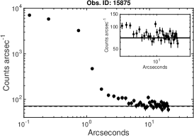
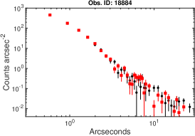
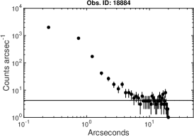
Figure 1: Left panel. Chandra 1-D radial profile from the Chandra CC-mode observation 15875. The black horizontal line represents the background level, while black-dots represent the radial profile. No extended emission is obvious beyond 5^′′ from the central brightest pixel. Middle panel. Chandra 2-D radial profile from the 2016 TE mode observation. The black-dots represent the data radial profile, while the red squares represent the Chart and MARX PSF simulation. The agreement between the profile and the PSF simulation indicates the absence of any extended emission around SGR J1935$+$2154. Right panel. Chandra 1-D radial profile after converting the TE-mode observation 18884 into a 1D CC-mode observation, as a verification of our results for the CC-mode observation 15875. See text for more details.

Two of the Chandra observations, including the one in 2016, were taken in TE mode, while the other two were taken in CC mode. For the two TE mode observations we simulated a Chandra PSF at the source position with the spectrum of SGR J1935$+$2154, using the Chandra ray-trace (ChaRT) and MARX. The middle panel of Figure 1 shows the radial profile of the 2016 TE mode observations, which had an exposure twice as long as the one taken on 2014. Black dots represent the radial profile of the actual observation, while the red squares represent the radial profile of the simulated PSF. There is no evidence for small-scale extended emission beyond a point source PSF in this observation. The 2014 observation showed similar results.

The CC-mode observations are not straightforward to perform imaging analysis with, given their 1-D nature. To mitigate this limitation, we calculated and averaged the total number counts in each two pixels at equal distance from the central brightest pixel, up to a distance of 20^′′ (we also split the central brightest pixel into two, to better sample the inner 0.5^′′). The background for these observations was estimated by averaging the number of counts from all pixels at a distance 25-50^′′ from both sides of the central brightest pixel. The left panel of Figure 1 shows the results of our analysis on the longest of the 2 CC-mode observations, obs. ID 15875 (notice the y-axis unit of counts arcsec^-1). The solid horizontal line represents the background level, while the dots represent the 1-D radial profile of SGR J1935$+$2154. The inset is a zoom-in at the $3-20$^′′ region. The level of emission beyond $\sim 5$^′′ from the central pixel is consistent with the background, hence, we conclude that there is no evidence for small-scale extended emission from the source. We verified our results by converting our 2016 TE-mode observation into a CC mode one by collapsing the counts into 1D. We then performed the same analysis on this converted image as the one done on the CC mode observations. The results are shown in the right panel of Figure 1. We note that these results are in contrast with the results presented in Israel et al. (2016b, see their Figure 1). We have not been able to identify the reason of this discrepancy.

XMM-Newton observations showed a weak extended emission after stacking all seven 2014 observations, in accordance with the results reported by Israel et al. (2016b).

3.2 Timing

3.2.1 X-ray

We searched the NuSTAR and Chandra data for the pulse period from SGR J1935$+$2154. We focused the search in an interval around the expected pulse period from the source at the NuSTAR and Chandra MJDs, after extrapolating the timing solution detected with Chandra and XMM-Newton during the 2014 outburst (Israel et al. 2016b). We included the possibility of timing noise and/or glitches and searched an interval with $\delta\dot{P}\approx 1.0\times 10^{-9}$ s s^-1. For the FPMA and FPMB modules, we extracted events from a circle with a 45^′′ radius around the source position, and in the energy range $3-50$ keV. We extracted the Chandra events using a 2^′′ circle centered at the source in the energy range $1-8$ keV. We barycenter-corrected the photon arrival times to the solar system barycenter.

We first applied the $Z^{2}_{m}$ test algorithm (Buccheri et al. 1983) at the NuSTAR data, where $m$ is the number of harmonics. Although the signal during the 2014 outburst was near-sinusoidal, we applied the test using $m=1,2,3,$ and $5$, considering the possibility of a change in the pulse shape during the later outbursts. The highest peak in the $Z^{2}$ power in the NuSTAR data, with a significance of $3.7\sigma$, is located at the period reported in Younes et al. (2015a) of 3.24729(1) s. This is largely different compared to the pulse-period of 3.24528(6) s derived by Israel et al. (2016b) for the 2015 XMM-Newton observation taken a month later. The change in frequency between the two observations is about $1.2\times 10^{-9}$ s s^-1; too large to correspond to any timing noise. We also repeated our above analysis for different energy cuts, namely $3-10$ keV and $3-30$ keV, and for different circular extraction regions of 30^′′ and 37^′′ radii (to optimize S/N). We find no other significant peaks in the $Z^{2}$ power for any of the above combinations. We, therefore, conclude that we do not detect the spin period of the source in our 2015 NuSTAR observation. Following the same method, we searched for the pulse period in the 2016 Chandra observation. Similarly, we do not detect the pulse period from SGR J1935$+$2154.

We estimated upper limits on the rms pulsed-fraction (PF) of a pure sinusoidal modulation by simulating 10,000 light curves with mean count rate corresponding to the true background-corrected count rate of the source and pulsed at a given rms PF. For our 2015 NuSTAR observation, we derive a $3\sigma$ ($99.73\%$ confidence) upper-limit on the rms PF of $26\%$, $35\%$, and $43\%$ in the energy ranges $3-50$ keV, $3-10$ keV, and $10-50$ keV, respectively. For our 2016 Chandra observation, we set a $3\sigma$ rms PF upper-limit of $8\%$. These limits are consistent with the $5\%$ rms pulsed fraction derived during the 2015 XMM-Newton observation in the 0.5-10 keV range (Israel et al. 2016b).

3.2.2 Radio

A consistent method of data analysis was adopted for both the C-band and L-band data analysis, and was based on tools from the pulsar search and analysis software PRESTO (Ransom 2001; Ransom et al. 2002, 2003). To excise radio frequency interference (RFI) we created a mask using rfifind. After RFI excision, we used two different techniques to search for radio pulsations: i) a search based on the known spin parameters from an X-ray derived ephemeris, and ii) a blind, Fourier-based periodicity search, as we describe below.

Ephemeris based search. Coherent X-ray pulsations from SGR J1935+2154 were detected by Israel et al. (2014) at a $>10\sigma$ confidence level. Upon this discovery, SGR J1935+2154 was monitored using XMM-Newton and Chandra observations between $2014-2015$ (see, Israel et al. 2016a). This campaign resulted in a timing solution as presented in Table 2 of Israel et al. (2016a). We used the period, period derivative and second period derivative from this ephemeris to extrapolate the source spin period for Obs. $1-3$ and Obs. $4-6$ ($3.2452679$ s, $3.2458097$ s, respectively). We then folded each C-band and L-band observation with the appropriate spin period using PRESTO’s prepfold. This folding operation was restricted to only optimize S/N over a search range in pulse period and incorporated the RFI mask. We repeated this folding routine over dispersion measures (DMs) ranging from $0$ to $1000$ pc cm^-3 in steps of $50$ pc cm^-3. Recently, using the intermediate flare from SGR J1935+2154 along with a magnetic field estimate from the timing analysis of Israel et al. (2016a), Kozlova et al. (2016) showed that the magnetar is at a distance of $<10$ kpc. We used the NE2001 Galactic electron density model and integrated in the source direction up to $10$ kpc to obtain an expected DM. We obtain a value of $344$ pc  cm^-3 (typical error is 20% fractional), which lies well within the DM range of our searches. These searches found no plausible radio pulsations from SGR J1935+2154.

Blind searches. We also conducted searches using no a priori assumption about the spin period in order to allow for a change compared to the ephemeris (e.g., a glitch) or the serendipitous discovery of a pulsar in the field. Using prepsubband, we created barycentered and RFI-excised time series for a DM range of $0$ to $1050$ pc cm^-3, where the trial DM spacing was determined using ddplan. We then Fourier transformed each time series with realfft and conducted accelsearch based searches (with a maximum signal drift of $z_{\rm max}=100$ in the power spectrum) in order to maintain sensitivity to a possible binary orbit. The most promising candidates from this search were collated and ranked using ACCEL_sift. We folded the raw filterbank data for the best 200 candidates identified with ACCEL_sift and then visually inspected each candidate signal using parameters such as cumulative S/N, S/N as a function of DM, pulse profile shape and broad-bandedness as deciding factors in judging whether a certain candidate was plausibly of astrophysical origin or whether it was likely to be noise or RFI. We found no plausible astrophysical signals in this analysis as well.

We estimate maximum flux density limits using the radiometer equation (see Dewey et al. 1985; Bhattacharya 1998; Lorimer & Kramer 2012) given by:

$$S_{min}=\frac{\left(\frac{S}{N}\right)~{}\beta~{}T_{sys}}{G~{}\sqrt{n_{p}~{}t_{obs}~{}\bigtriangleup f}}~{}\sqrt{\frac{W}{P-W}}$$ (1)

where, $G$ is the gain of the telescope (K Jy^-1), $\beta$ is a correction factor which is $\sim 1$ for large number of bits per sample, $T_{sys}$ is the system noise temperature (K), $\bigtriangleup f$ is the bandwidth (MHz), and $t_{obs}$ is the integration time (s) for a given source. These parameters for the observational setup in each band are listed in Table 2. We assume a pulsar duty cycle ($W/P$) of $20\%$ and a minimum detectable signal-to-noise ratio of $10$ in our search. This yields a maximum flux density limit of $14$ $\mu$Jy for the C-band observations and $7$ $\mu$Jy for the L-band observations.

3.3 X-ray spectroscopy

We fit our spectra in the energy range $0.8-8$ keV for Chandra, $0.8-10$ keV for XMM-Newton and Swift, and $3-79$ keV for NuSTAR, using XSPEC (Arnaud 1996) version 12.9.0k. We used the photoelectric cross-sections of Verner et al. (1996) and the abundances of Wilms et al. (2000) to account for absorption by neutral gas. For all spectral fits using different instruments, we added a multiplicative constant normalization, frozen to 1 for the spectrum with the highest signal to noise, and allowed to vary for the other instruments. This takes into account any calibration uncertainties between the different instruments. We find that this uncertainty is between $2-8\%$. For all spectral fitting, we used the Cash-statistic in XSPEC for model parameter estimation and error calculation, while the goodness command was used for model comparison. All quoted uncertainties are at the $1\sigma$ level, unless otherwise noted.

3.3.1 The 2014 outburst

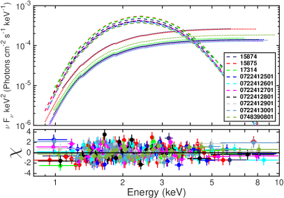
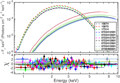
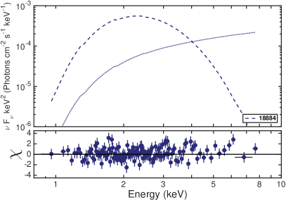
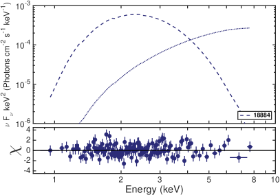
Figure 2: Upper panels. BB+PL (left) and BB+BB (right) fits to the Chandra and XMM-Newton spectra from the 2014 outburst. Lower panels. BB+PL (left) and BB+BB (right) fits to the Chandra spectrum from the 2016 outburst. The best-fit spectral components are shown in $\nu F_{\nu}$ space, while residuals are shown in terms of $\chi$. See text and table 3 for details.

We started our spectral analysis of the 2014 outburst (Table LABEL:logObs) by focusing on the high S/N ratio spectra derived from the 7 XMM-Newton observations (PN+MOS1+MOS2). Firstly, we fit these spectra simultaneously with an absorbed (tbabs in XSPEC) blackbody plus power-law (BB+PL) model, allowing all spectral model parameters to vary freely, i.e., BB temperature (kT) and emitting area, and PL photon index ($\Gamma$) and normalization, except for the absorption hydrogen column density, which we linked between all spectra. This model provides a good fit to the data with a C-stat of 5116.7 for 5196 degrees of freedom (d.o.f.). We find a hydrogen column density $N_{\rm H}=(2.4\pm 0.1)\times 10^{22}$ cm^-2. The BB temperatures and PL indices are consistent for all spectra within the $1\sigma$ level. Hence, we linked these parameters and re-fit. We find a C-stat of 5131.75 for 5208 d.o.f. To estimate which model is preferred by the data (here and elsewhere in the text), we estimate the difference in the Bayesian Information Criterion (BIC), where $\Delta BIC$ of 8 is considered significant and the model with the lower $BIC$ is preferred (e.g., Liddle 2007). Comparing the case of free versus linked $kT$ and $\Gamma$, we find that the case of linked parameters is preferred with a $\Delta BIC\approx 88$. This fit resulted in a hydrogen column density $N_{\rm H}=2.4\pm 0.1\times 10^{22}$ cm^-2, a BB temperature $kT=0.46\pm 0.01$ keV and area $R=1.45_{-0.03}^{+0.07}$ km, and a photon index $\Gamma=2.0_{-0.5}^{+0.4}$.

Table 3: Best-fit XMM-Newton and Chandra X-ray spectral parameters

Obs. ID	$N_{\rm H}$	$kT_{\rm cool}$	$R_{\rm cool}^{a}$	$\Gamma$/$kT_{\rm hot}$	$R_{\rm hot}^{a}$	$F_{\rm kT-cool}$	$F_{\rm PL/kT-hot}$
	cm-2	(keV)	(km)	(/keV)	($10^{-3}$ km)	($10^{-12}$, erg s-1 cm-2)	($10^{-12}$, erg s-1 cm-2)
2014 Outburst – BB+PL
15874	$2.46\pm 0.08$	$0.47\pm 0.01$	$1.7\pm 0.08$	$2.0\pm 0.2$	…	$1.78\pm 0.16$	$1.31\pm 0.33$
15875	(L)	(L)	$1.8\pm 0.05$	(L)	…	$2.01\pm 0.09$	$1.27\pm 0.27$
17314	(L)	(L)	$1.8\pm 0.06$	(L)	…	$1.96\pm 0.08$	$0.75\pm 0.19$
0722412501	(L)	(L)	$1.6\pm 0.05$	(L)	…	$1.50\pm 0.06$	$0.69\pm 0.17$
0722412601	(L)	(L)	$1.6\pm 0.05$	(L)	…	$1.49\pm 0.06$	$0.62\pm 0.15$
0722412701	(L)	(L)	$1.6\pm 0.05$	(L)	…	$1.56\pm 0.06$	$0.64\pm 0.16$
0722412801	(L)	(L)	$1.6\pm 0.06$	(L)	…	$1.57\pm 0.07$	$0.69\pm 0.17$
0722412901	(L)	(L)	$1.6\pm 0.06$	(L)	…	$1.50\pm 0.08$	$0.65\pm 0.17$
0722413001	(L)	(L)	$1.5\pm 0.05$	(L)	…	$1.42\pm 0.07$	$0.66\pm 0.17$
0748390801	(L)	(L)	$1.5\pm 0.05$	(L)	…	$1.38\pm 0.09$	$0.90\pm 0.21$
2016 Outburst
18884	$2.7\pm 0.3$	$0.42\pm 0.04$	$2.3\pm 0.5$	$1.3_{-0.7}^{+0.9}$	…	$2.0\pm 0.3$	$1.1\pm 0.6$
2014 Outburst – BB+BB
15874	$2.30\pm 0.04$	$0.48\pm 0.01$	$1.8\pm 0.6$	$1.6\pm 0.1$	$80\pm 9$	$2.12\pm 0.09$	$0.53\pm 0.08$
15875	(L)	(L)	$1.9\pm 0.6$	(L)	$79\pm 9$	$2.34\pm 0.05$	$0.52\pm 0.03$
17314	(L)	(L)	$1.8\pm 0.6$	(L)	$61\pm 8$	$2.10\pm 0.06$	$0.31\pm 0.04$
0722412501	(L)	(L)	$1.6\pm 0.5$	(L)	$57\pm 7$	$1.66\pm 0.04$	$0.27\pm 0.02$
0722412601	(L)	(L)	$1.5\pm 0.6$	(L)	$54\pm 7$	$1.62\pm 0.04$	$0.25\pm 0.02$
0722412701	(L)	(L)	$1.6\pm 0.5$	(L)	$55\pm 7$	$1.70\pm 0.04$	$0.25\pm 0.02$
0722412801	(L)	(L)	$1.6\pm 0.5$	(L)	$57\pm 7$	$1.72\pm 0.05$	$0.28\pm 0.03$
0722412901	(L)	(L)	$1.6\pm 0.6$	(L)	$55\pm 8$	$1.65\pm 0.05$	$0.26\pm 0.03$
0722413001	(L)	(L)	$1.5\pm 0.6$	(L)	$56\pm 7$	$1.57\pm 0.04$	$0.26\pm 0.03$
0748390801	(L)	(L)	$1.5\pm 0.6$	(L)	$65\pm 8$	$1.62\pm 0.05$	$0.36\pm 0.03$
2016 Outburst
18884	$2.7\pm 0.3$	$0.43\pm 0.02$	$2.3\pm 0.4$	$2.0_{-0.5}^{+1.3}$	$52_{-26}^{+36}$	$2.5\pm 0.3$	$0.45_{-0.06}^{-0.07}$

• Fluxes are derived in the energy range 0.5-10 keV. ^a Assuming a distance of 9 kpc.

We then fit the three Chandra spectra simultaneously, linking the hydrogen column density, while leaving all other fit parameters free to vary. We find a common hydrogen column density $N_{\rm H}=(2.9\pm 0.3)\times 10^{22}$ cm^-2. Similar to the case of the XMM-Newton observations, the BB temperature and the PL photon index were consistent within the 1$\sigma$ confidence level among the three observations. We, therefore, linked the BB temperature and the PL photon index in the three observations and found $kT=0.46\pm 0.02$, $R=1.8\pm 0.2$ km, and $\Gamma=2.4_{-0.6}^{+0.4}$.

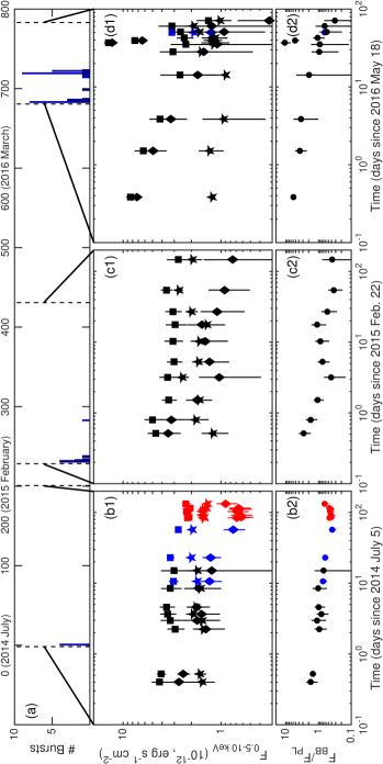
Figure 3: SGR J1935$+$2154 BB+PL spectral evolution during the 2014, 2015, and May and June 2016 outbursts. Panel (a) shows the number of bursts detected by the Inter Planetary Network (IPN) since the source discovery and up to August 2016. Panels (b1) , (c1), and (d1), represent the evolution of the BB (stars), PL (diamonds), and total fluxes (squares) from outburst onset and up to 200 days. Panels (b2) , (c2), and (d2), represent the evolution of the $F_{\rm PL}/F_{\rm BB}$ ratio. Colors represent fluxes derived from different instruments (black:Swift, blue:Chandra, red:XMM-Newton). See text for details.

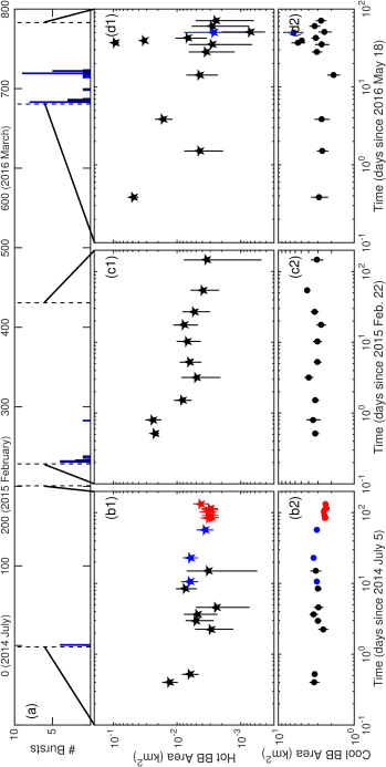
Figure 4: SGR J1935$+$2154 BB+BB spectral evolution during the 2014, 2015, and May and June 2016 outbursts. Panel (a) shows the number of bursts detected by the Inter Planetary Network (IPN) since the discovery and up to August 2016. Panels (b1) , (c1), and (d1), represent the evolution of the hot BB area from outburst onset and up to 200 days. Panels (b2) , (c2), and (d2), represent the evolution of the cool BB area. Colors represent values derived from different instruments (black:Swift, blue:Chandra, red:XMM-Newton). See text for more details.

Given the consistency in $N_{\rm H}$, BB temperature and PL photon index between the Chandra and XMM-Newton observations, we then fit the spectra from all 10 observations simultaneously, first, only linking the $N_{\rm H}$ among all observations. We find a good fit with a C-stat of 5750 for 5845 d.o.f, with $N=(2.4\pm 0.1)\times 10^{22}$ cm^-2. Similar to the above two cases, we find that the BB temperatures and the PL indices are consistent within 1$\sigma$. Hence, we fit all 10 observations while linking $KT$ and $\Gamma$. We find a C-stat of 5806 for 5863 d.o.f. Comparing this fit to the above case, we find a $\Delta BIC$=100, suggesting that the latter fit is preferred over the fit where parameters were left free to vary. The best fit spectral parameters for the BB+PL model are summarized in Table 3, while the data and best fit model are shown in Figure 2.

We also fit all spectra with an absorbed BB+BB model following the above methodology. We first only link $N_{\rm H}$ among all spectra while allowing the temperature and emitting area of the 2 BBs free to vary. We find that the BB temperature of the cool component as well as the hot component are consistent at the $1\sigma$ among all 10 observations, and were, therefore, linked. This alternative fit resulted in a C-stat of 5812 for 5863 d.o.f, similar in goodness to the BB+PL fit. Table 3 gives the BB+BB best fit spectral parameters while the data and best fit model are shown in Figure 2.

We analyzed the Swift/XRT observations taken during the 2014 outbursts following the procedure explained in Section 2.3. We fit all XRT spectra simultaneously with the BB+PL and BB+BB models. Due to the limited statistics, we fixed the temperatures and the photon indices to the values derived with the above XMM-Newton+Chandra fits. We made sure that the resulting fit was statistically acceptable using the XSPEC goodness command. In the event of a statistically bad fit, we allowed the temperatures and the photon indices to vary within the $3\sigma$ uncertainty of the XMM-Newton+Chandra fits, which did give a statistically acceptable fit in all cases. We show in Figure 3 the flux evolution of the BB+PL model and in Figure 4 the areas evolution of the 2BB model. These results are discussed in Section 4.

Finally, we note that during the 2015 outburst, which will be discussed in Section 3.3.2, NuSTAR reveals a hard X-ray component dominating the spectrum at energies $>10$ keV and with a non-negligible contribution at energies $5-10$ keV. In order to understand the effect of such a hard component on the spectral shape below $10$ keV (if it indeed exists during the 2014 outburst), we added a hard PL component to the two above models (i.e., BB+PL and 2BB) while fitting the 7 XMM-Newton observations. We fixed its index and normalization to the result of a PL fit to the NuSTAR data from $10-79$ keV. As one would expect, we find that the addition of this extra hard PL results in a softening of the $<10$ keV PL and hot BB components. On average, we find a photon index for the soft PL $\Gamma=2.7\pm 0.3$. For the 2BB model, we find a temperature for the hot BB $kT=0.8\pm 0.2$ with a radius for the emitting area $R\approx 210\pm 30$ m. Moreover, we find the fluxes of the low energy PL or the hot BB to be a factor of $\sim$3 lower, however, the total $0.5-10$ keV flux is similar to the above 2 models when we did not include contribution from a hard PL. We cannot, unfortunately, add a hard PL component to the XRT spectra and still extract meaningful flux values from the 2 other components $<10$ keV, due to very limited statistics. A complete statistical analysis, invoking many spectral simulations, aiming at understanding the exact effect of a hard PL component to the spectral curvature $<10$ keV is beyond the scope of this paper. In all our discussions in Section 4, however, we made sure to avoid making any conclusions that could be affected by such a shortcoming of the data we are considering here.

3.3.2 The 2015 outburst

For the 2015 outburst, we first concentrated on the analysis of the simultaneous NuSTAR and Swift/XRT observations (Table LABEL:logObs) taken on February 27, 5 days following the outburst onset. This provided the first look at the broad-band X-ray spectrum of the source. SGR J1935$+$2154 is clearly detected in the two NuSTAR modules with a background-corrected number of counts of $\sim 800$ ($3-79$ keV). We find a background-corrected number of counts in the $3-10$ keV and $10-79$ keV of about $500$ and $300$ counts, respectively. The simultaneous XRT observation provided about 130 background-corrected counts in the energy range $0.5-10$ keV.

We then fit the spectra simultaneously to an absorbed BB+PL model. We find a good fit with a C-stat of 444 for 452 d.o.f., with an $N_{\rm H}=(2\pm 0.7)\times 10^{22}$ cm^-2. We find a BB temperature $kT=0.51\pm 0.04$, a BB emitting area radius $R=1.4\pm 0.3$ km, and a PL photon index $\Gamma=0.9\pm 0.1$. This spectral fit results in a $0.5-10$ keV and $10-79$ keV absorption corrected fluxes of $(2.6\pm 0.4)\times 10^{-12}$ erg s^-1 cm^-2 and $(3.7\pm 0.4)\times 10^{-12}$ erg s^-1 cm^-2, respectively. Table 4 summarizes the best fit model parameters while Figure 5 shows the data and best fit model components in $\nu F\nu$ space (upper-panel) and the residuals in terms of $\sigma$ (lower-panel).

Since the Chandra and XMM-Newton 2014 spectra were best fit with a 2-component model below $10$ keV, we added a third component to the Swift+NuSTAR data, a BB or a PL. Such a three model component is required for many bright magnetars to fit the broad-band $0.5-79$ keV spectra (e.g., Hascoët et al. 2014). For SGR J1935$+$2154, the addition of either component does not significantly improve the quality of the fit, both resulting in a C-stat of 441 for 450 d.o.f. To understand whether our Swift+NuSTAR data are of high enough S/N to exclude the possibility of a 3 model component, we simulated 10,000 Swift-XRT and NuSTAR spectra with their true exposure times, based on the 2014 $0.5-10$ keV spectrum and including a hard PL component as measured above. We find that we cannot retrieve all three components at the $3\sigma$ level; most of these simulated spectra are best fit with a 2 model component, namely an absorbed PL+BB. We, hence, conclude that our Swift+NuSTAR data do not require the existence of a 3 component model for the broad-band spectrum of SGR J1935$+$2154.

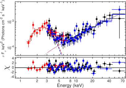
Figure 5: Upper panel. Simultaneous broad-band NuSTAR and Swift-XRT spectra of SGR J1935$+$2154 taken on 2015 February 27, 5 days after the 2015 outburst onset. Dots, squares, and diamonds are the NuSTAR FPMA, FPMB, and Swift-XRT spectra, respectively. The solid lines represent the absorbed BB+PL best fit model in $\nu F\nu$ space, while the dashed and dotted lines represent the BB and PL components, respectively. Lower panel. Residuals of the best fit are shown in terms of standard deviation.

Table 4: Best-fit spectral parameters to the 2015 simultaneous Swift-XTR and NuSTAR spectra.

BB+PL
$N_{\rm H}$ ($10^{22}$ cm-2)	$2_{-0.7}^{+0.8}$
$kT$ (keV)	$0.51\pm 0.04$
$R_{\rm cool}^{a}$ (km)	$1.4_{-0.3}^{+0.5}$
$F_{\rm BB}$ ($10^{-12}$ erg s-1 cm-2)	$2.0_{-0.4}^{+0.5}$
$\Gamma$	$0.9\pm 0.1$
$F_{\rm PL}$ ($10^{-12}$ erg s-1 cm-2)	$4.2_{-0.7}^{+0.8}$
$F_{\rm 0.5-10~{}keV}$ ($10^{-12}$ erg s-1 cm-2)	$2.6\pm 0.4$
$F_{\rm 10-79~{}keV}$ ($10^{-12}$ erg s-1 cm-2)	$3.7_{-0.5}^{+0.4}$
$L_{\rm 0.5-79keV}^{a}$ ($10^{34}$ erg s-1)	$6.1\pm 0.4$

• ^aAssuming a distance of 9 kpc.

To study the spectral evolution of the source during its 2015 outburst, we fit the Swift/XRT spectra of observations taken after 2015 February 22 (Table LABEL:logObs) with an absorbed BB+PL and a 2BB models. We fixed the absorption column density, temperatures and the photon index to the values derived with the 2014 XMM-Newton+Chandra fits, but allowed for them to vary within their $3\sigma$ uncertainties in the case of a statistically bad fit. We show in Figure 3 the flux evolution of the BB+PL model and in Figure 4 the areas evolution of the 2BB model. These results are discussed in Section 4.

3.3.3 The 2016 outburst

We started our spectral analysis of the 2016 outburst with the Chandra observation taken on July 07. Similar to the high S/N spectra from the 2014 and 2015 outbursts, an absorbed BB or PL spectral model fails to describe the data adequately. Hence, we fit an absorbed BB+PL and a 2BB model to the data. Both models result in equally good fits with a C-stat of 289 for 302 d.o.f. The best fit model parameters are shown in Table 3, while the models in $\nu F_{\nu}$ space and deviations of the data from the model in terms of $\sigma$ are shown in Figure 5. These spectral parameters are within $1\sigma$ uncertainty from the parameters derived during the 2014 and 2015 outbursts.

SGR J1935$+$2154 was observed regularly after the May outburst of 2016 with Swift. These observations also covered its 2016 June outburst. We analyzed all XRT observations taken during this period, and fit all spectra with an absorbed BB+PL and 2BB models. We froze the absorption hydrogen column density $N_{\rm H}$, $\Gamma$ and $kT$ to the best fit values as derived during the 2014 outburst. The evolution of the flux for the BB+PL model and the emitting area radius of the 2BB model are shown in Figures 3 and 4, respectively.

3.4 Outburst comparison and evolution

We first concentrate on the 2014 outburst which has the best observational coverage compared to the rest. The outburst decay is best fit with an exponential function $F(t)=Ke^{-t/\tau}+F_{\rm q}$, where $K$ is a normalization factor, while $F_{\rm q}=2.1\times 10^{-12}$ erg s^-1 cm^-2 is the quiescent flux level derived with the XMM-Newton observations (Figure 6). This fit results in a characteristic decay time-scale $\tau_{\rm 14}=29\pm 4$ days (Table 5). Integrating over 200 days, we find a total energy in the outburst, corrected for the quiescent flux level, $E_{\rm 14}=(4.1\pm 0.7)\times 10^{40}$ erg. We find a flux at outburst onset $F_{\rm on-14}=(4.3\pm 0.7)\times 10^{-12}$ erg s^-1 cm^-2, and a ratio to the quiescent flux level $R_{\rm 14}\approx 2.0$. Following the same recipe for the 2015 outburst, we find a characteristic decay time-scale $\tau_{\rm 15}=43^{+12}_{-8}$ days, and a total energy in the outburst, corrected for the quiescent flux level, $E_{\rm 15}=(6.1\pm 1.1)\times 10^{40}$ erg. The flux at outburst onset is $F_{\rm on-15}=(4.7\pm 0.08)\times 10^{-12}$ erg s^-1 cm^-2, and its ratio to the quiescent flux level $R_{\rm 15}=2.2$.

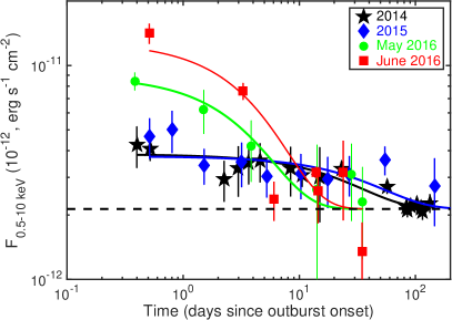
Figure 6: Total $0.5-10$ keV flux evolution with time for all four outbursts detected from SGR J1935$+$2154. The flux level reached highest at outburst onset during the latest outburst of June 2016, during which the most number of bursts have been detected from the source. Solid lines represent an exponential-decay fit. See text for details.

A similar analysis for the May and June 2016 outbursts was difficult to perform due to the lack of observations $\sim 30$ days beyond the start of each outburst (Figure 6), and the poor constraints on the fluxes (due to the short XRT exposures) derived few days after the outburst onset. These fluxes are consistent with $F_{\rm q}$ and the slightly brighter flux level seen in the 2014 and 2015 outbursts between few days after outburst onset and quiescence reached $\sim 70$ days later. Hence, we cannot derive the long term decay shape of the lightcurve during the last two outbursts from SGR J1935$+$2154.

Table 5: Outburst properties

Outburst	$\tau$	$K$	$E_{\rm 10}^{a}$	$E_{\rm 200}^{b}$	$F_{\rm peak}$	$E_{\rm burst}^{c}$
	(days)	($10^{-12}$)	($10^{40}$ erg)	($10^{40}$ erg)	($10^{-12}$ erg s-1 cm-2)	($10^{38}$ erg s-1)
2014	$29\pm 4$	$1.7\pm 0.2$	$1.2\pm 0.3$	$4.1\pm 0.7$	$4.3\pm 0.7$	$8\pm 2$
2015	$43^{+12}_{-8}$	$1.6_{-0.3}^{+0.4}$	$1.2\pm 0.2$	$6.1\pm 1.1$	$4.7\pm 0.8$	$83\pm 3$
2016 Mayd	$3.7\pm 1.0$	$6.8_{-0.5}^{+0.7}$	$2.0\pm 0.3$	NA	$8.5\pm 0.6$	$411\pm 3$
2016 Juned	$4.3\pm 1.0$	$10.8_{-2.5}^{+3.2}$	$3.6\pm 0.4$	NA	$14\pm 1$	$1020\pm 8$

• All energies are derived assuming a distance of 9 kpc. ^a Integrated total energy within 10 days from outburst onset. ^b Integrated total energy within 200 days from outburst onset. ^c Total energy in the bursts for the day of the outburst onset, i.e., 2014 July 05, 2015 February 22, 2016 May 18, 2016 June 23 (Lin et al. in prep.). ^d Long-term outburst behavior during 2016 cannot be explored due to lack of high S/N observations beyond few days of outburst onset. See text for details.

However, an exponential decay fit to the 2016 outbursts results in short term characteristic time-scales $\tau_{\rm May-16}\approx\tau_{\rm June-16}\approx 4$ days, indicating a quick initial decay which might have been followed by a longer one similar to what is observed in 2014 and 2015. To enable comparison between all outbursts, we derive the total energy emitted within 10 days of each outburst. These are reported in Table 5. The 2016 outburst onset to quiescence flux ratios are $R_{\rm May16}=4.0$ and $R_{\rm June16}=6.7$. Table 5 also includes the total energy in the bursts during the first day of each of the outbursts (Lin et al. in prep.).

Finally, we note that the last observation during the May 2016 outburst was taken 1.5 days prior to the start of the June outburst (last green dot and first red square in Figure 6). The total fluxes from the two observations differ at the $\gtrsim 5\sigma$ level. These results are discussed in Section 4.2.

4 Discussion

4.1 Broad-band X-ray properties

Using high S/N ratio observations, we have established that the SGR J1935$+$2154 soft X-ray spectrum, with photon energies $<10$ keV, is well described with the phenomenological BB+PL or 2BB model. NuSTAR observations, on the other hand, were crucial in providing the first look at this magnetar at energies $>10$ keV, revealing a hard X-ray tail extending up to $79~{}$keV. We note that this NuSTAR observation was taken 5 days after the 2015 outburst. The simultaneous Swift+NuSTAR fit revealed a $0.5-10$ keV flux $\sim 40\%$ larger than the quiescent flux, which we assume it to be at the 2014 XMM-Newton level of $2.2\times 10^{-12}$ erg s^-1 cm^-2. The spectra below 10 keV did not show significant spectral variability during any of the outbursts (Section 4.2), except for the relative brightness. Accordingly, one can conjecture that SGR J1935$+$2154 has a similar high-energy tail during quiescence, though proof of such requires further dedicated monitoring of the source with NuSTAR or INTEGRAL.

The presence of hard-X-ray tails, such as exhibited by SGR J1935$+$2154, is clearly seen in about a third of all known magnetars (e.g., Kuiper et al. 2006; den Hartog et al. 2008b; Enoto et al. 2010; Esposito et al. 2007), but may indeed be universal to them. Spectral details differ across the population. For instance, the hard X-ray tail photon index we measure, $\Gamma_{\rm H}\approx 0.9$, is quite similar to some measured for AXPs (e.g., An et al. 2013; Vogel et al. 2014; Tendulkar et al. 2015; den Hartog et al. 2008a), but somewhat harder than other sources (e.g., Esposito et al. 2007; Yang et al. 2016). Moreover, the flux in the hard PL tail is 2 times larger than the flux in the soft components. This flux ratio varies by about 2 orders of magnitude among the magnetar population (Enoto et al. 2010).

Kaspi & Boydstun (2010, see also ) searched for correlations between the observed X-ray parameters and the intrinsic parameters for magnetars. They found an anti-correlation between the index differential $\Gamma_{\rm S}-\Gamma_{\rm H}$ and the strength of the magnetic field $B$. For SGR J1935$+$2154, with its spin-down field strength of $B=2.2\times 10^{14}$ G (Israel et al. 2016b), the determination here of $\Gamma_{\rm S}-\Gamma_{\rm H}\approx 1.0-2.0$ nicely fits the Kaspi & Boydstun (2010) correlation. Moreover, Enoto et al. (2010) noted a strong correlation between the hardness ratio, defined as $F_{\rm H}/F_{\rm S}$ for the hard and soft energy bands, respectively, and the characteristic age $\tau$. Following the same definition for the energy bands as in Enoto et al. (2010), we find $F_{\rm H}/F_{\rm S}\approx 1.8$ which falls very close to this correlation line given the SGR J1935$+$2154 spin-down age $\tau=3.6$ Kyr (Israel et al. 2016b). Since the electric field for a neutron star $E$ along its last open field line is nominally inversely proportional to the characteristic spin down age $E=\Omega RB\propto\tau^{-1/2}$, Enoto et al. (2010) argued that a younger magnetar will be able to sustain a larger current, accelerating more particles into the magnetosphere and causing a stronger hard X-ray emission in the tail. This scenario is predicated on the conventional picture of powerful young rotation-powered pulsars like the Crab.

The most discussed model for generating a hard X-ray tail in magnetar spectra is resonant Compton up-scattering of soft thermal photons by highly relativistic electrons with Lorentz factors $\sim 10-10^{4}$ in the stellar magnetosphere (e.g., Baring & Harding 2007; Fernández & Thompson 2007; Beloborodov 2013). The emission locale is believed to be at distances $\sim 10-100R_{\hbox{\sixrm NS}}$ where $R_{\hbox{\sixrm NS}}=10~{}$km is the neutron star radius. There the intense soft X-ray photon field seeds the inverse Compton mechanism, and the collisions are prolific because of scattering resonances at the cyclotron frequency and its harmonics in the rest frame of an electron. Magnetar conditions guarantee that electrons accelerated by voltages in the inner magnetosphere will cool rapidly down to Lorentz factors $\gamma\sim 10-10^{2}$ (Baring et al. 2011) due to the resonant scatterings. Along each field line, the up-scattered spectra are extremely flat, with indices $\Gamma_{h}\sim-0.5$ – $0.0$ (Baring & Harding 2007, see also Wadiasingh, et al., in prep.), though the convolution of contributions from extended regions is necessarily steeper, and more commensurate with the observed hard tail spectra (Beloborodov 2013). While the inverse Compton emission can also extend out to gamma-ray energies, the prolific action of attenuation mechanisms such as magnetic pair creation $\gamma\to e^{+}e^{-}$ and photon splitting $\gamma\to\gamma\gamma$ (Baring & Harding 2001) limits emergent signals to energies below a few MeV in magnetars (Story & Baring 2014), and probably even below 500 keV.

Beloborodov (2013, see also ) developed a coronal outflow model based on the above picture, using the twisted magnetosphere scenario (Thompson et al. 2002; Beloborodov 2009). Twists in closed magnetic field loops (dubbed $J$-bundles) extending high into the magnetosphere can accelerate particles to high Lorentz factors, which will decelerate and lose energy via resonant Compton up-scattering. If pairs are created in profusion, they then annihilate at the top of a field loop. Another one of the $J$-bundle model predictions is a hot spot on the surface formed when return currents hit the surface at the footprint of the twisted magnetic field lines. The physics in this model is mostly governed by the field lines twist amplitude $\psi$ (Thompson et al. 2002), the voltage $\Phi_{j}$ in the bundle, and its half-opening angle to the magnetic axis $\theta_{\rm j}$ (Beloborodov 2013; Hascoët et al. 2014).

The temperatures expected for the hotspots are of the order of $\sim 1$ keV while areas depend on the geometry of the bundle and the angle $\theta_{j}$. For a dipole geometry, $A_{\rm j}\sim(1/4)\theta_{\rm j}^{2}A_{\rm ns}\approx 0.02(\theta_{\rm j}/0.3)^{2}A_{\rm ns}$, where $A_{\rm ns}=4\pi R_{\odot}^{2}$ is the NS surface area (Hascoët et al. 2014). Assuming that the hot BB in our model discussed in the last paragraph of Section 3.3.1 represents the footprints of the $J$-bundle, for which we find a temperature $kT=0.8$ keV, we estimate its surface area $A\approx 0.6$ km². Assuming that $A\approx A_{\rm j}$, we estimate $\theta_{\rm j}\approx 0.05$.

The above calculation assumes that the $J$-bundle is axisymmetric extending all around the NS. The hot-spot, hence, is a ring around the polar cap rim. The smaller area that we derive may suggest that the $J$-bundle is not axisymmetric and extends only around part of the NS, implying that the twist could have been imparted onto local magnetic field lines.

The total power dissipated by the $J$-bundle in the twisted magnetosphere model can be expressed as $L_{\rm j}\approx 2\times 10^{35}\psi\Phi_{\rm 10}\mu_{\rm 32}R_{\rm 10}\theta_{\rm j,0.3}^{4}$ erg s^-1 (equation 3, Hascoët et al. 2014), where $\Phi_{\rm 10}$ is the voltage in units of $10^{10}$ V, $\mu_{\rm 32}$ is the magnetic moment in units of $10^{32}$ G cm³, $R_{\rm 10}$ is the NS radius in units of 10 km, and $\theta_{\rm j,0.3}=\theta_{\rm j}/0.3$. Given the magnetic moment of SGR J1935$+$2154, for choices of $\phi_{\rm 10}=1$, $\psi=1$, $R_{\rm 10}=1$, and $\theta_{\rm j,0.3}\approx 0.2$, we estimate $L_{\rm j}=7\times 10^{32}$ erg s^-1. This luminosity is a factor of $\sim 30$ smaller than the hard tail PL luminosity, $L_{\rm PL}=2.0\times 10^{34}$ erg s^-1 we derive with the NuSTAR data, after normalizing it to the 2014 XMM-Newton flux level. This might imply a larger voltage across the twisted field lines than the choice of $\phi_{10}=1$, which corresponds to only $\sim 3\times 10^{-6}$ times the open field line pole-to-equator voltage $2\pi R_{\hbox{\sixrm NS}}^{2}B_{p}/(Pc)\approx 2.8\times 10^{16}$ V for SGR J1935$+$2154. Another possibility is that the hard PL tail could be much fainter during quiescence, which might indicate a different decay trend for the high-energy tail compared to the 0.5-10 keV spectrum. A deep XMM-Newton+NuSTAR observation of SGR J1935$+$2154 during quiescence would help reveal the exact shape and power of the hard PL tail, inform on how activation relates to heat transfer to and from the stellar surface layers, and help refine the twisted magnetosphere model.

4.2 Outbursts

Since its discovery in June 2014, SGR J1935$+$2154 has shown four major bursting episodes, which culminated with the strongest one to date in June 2016. Similar to most other magnetars, SGR J1935$+$2154 bursting activity was accompanied by a persistent emission outburst, showing an increase in the flux level at, or shortly after, the onset of the bursting activity that decayed quasi-exponentially back to quiescence (e.g., Woods et al. 2004; Scholz et al. 2012; Göğüş et al. 2010; Kargaltsev et al. 2012; Coti Zelati et al. 2015; Younes et al. 2015b; Rea & Esposito 2011).

The rise time of magnetar outbursts is a challenging observational property to identify and quantify due to the randomness of the process. Magnetars are usually observed by pointed X-ray telescopes after they have entered a bursting episode. Hence, it is unclear whether magnetars show any persistent flux enhancement prior to the bursting activity, or whether the two happen (quasi-) simultaneously. CXOU J164710.2$-$455216 is the closest we have come to answering the above question. While being monitored with X-ray instruments, CXOU J164710.2$-$455216 was observed with XMM-Newton 5 days prior to bursting activity (Israel et al. 2007). The flux of this observation was consistent with quiescence while the following observation, which took place less than a day after the bursts, showed an increase by a factor of $\sim 300$. Similarly, SGR J1935$+$2154 was observed $\sim$1.5 days prior to its strongest bursting activity in 2016 June, while being monitored for its 2016 May activation. The latter observation showed a flux level close to quiescence, and was $5\sigma$ away from the flux measured at the start of the June 2016 outburst (Section 3.4). This implies that any instability invoked to explain the outbursts in magnetars has to develop on very short time-scales ($\lesssim 2$ days, e.g., Li et al. 2016).

The $0.5-10$ keV persistent flux level of SGR J1935$+$2154 at or shortly after the onset of the bursting activity varied in concordance with the bursting level from the source (see also, e.g., 1E 1547.0-5408, Ng et al. 2011). The source flux reached its highest level at the start of the 2016 June outburst, a factor of 7 that of the quiescent level (Figure 6). At the same time, the flux of the PL or the hot BB components (Figures 3 and 4), increased by a factor of $\sim 25$ compared to quiescence. The cold BB on the other hand, with a temperature of $kT=0.48$ keV and radius $R=1.8$ km, remained more or less constant throughout all four outbursts. Such a cold BB could be the result of internal heating of a large fraction of the magnetar surface (Thompson & Duncan 1996; Beloborodov & Li 2016).

The 2014 and 2015 flux decays followed a simple exponential trend with time-scales of $\sim 30-40$ days. The brighter 2016 outbursts, however, exhibited a quick decay trend on time-scales of $\sim 4$ days. Such fast initial drop in flux is seen at the outburst onset of a number of magnetars (e.g., SGR J1627$-$41, An et al. 2012; Swift J1834.9$-$0846, Kargaltsev et al. 2012, Swift J1822.3$-$1606, Scholz et al. 2012).

Similar amount of energy was emitted in the 2014 and 2015 outbursts (within $2\sigma$), $E\sim 5\times 10^{40}$ erg s^-1. We were only able to quantify the total energy emitted during the first 10 days of the May and June 2016 outbursts, $E=2\times 10^{40}$ erg s^-1 and $E=3.6\times 10^{40}$ erg s^-1, respectively. The energetics in these outbursts are at the lower end compared to the bulk of magnetar outbursts (Rea & Esposito 2011). We note that the energy in the bursts for the 4 outbursts varied by more than 2 orders of magnitude (Table 5, Lin et al. 2017 in prep.); a much larger increase than the energy emitted in the outbursts. For instance, the 2014 and 2015 ratio of total energy in the outbursts to total energy in bursts decreased from 50 to 8.

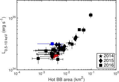
Figure 7: Total $0.5-10$ keV flux versus hot BB area from all outbursts of SGR J1935$+$2154. See also Figure 4.

Two models have been discussed in the context of magnetar outbursts. The first invoked an instability (external or internal) that rapidly (within few days) deposits energy, of the order of $10^{40}-10^{42}$ erg s^-1, at the crust level of the neutron star (e.g., Lyubarsky et al. 2002; Pons & Rea 2012; Brown & Cumming 2009). The depth at which the heat is deposited governs the outburst decay time-scale, which can range from weeks to months, as the crust cools back to its pre-outburst level. This timescale may also reflect the magnetic colatitude of the energy dissipation locale, as heat conductivity across strong fields is suppressed, so that vertical transport of energy is easier in polar activation zones. This picture fits the observed properties of the 2014 and 2015 outbursts of SGR J1935$+$2154. It is, however, difficult to reconcile the initial quick decay of a few days observed in the 2016 outbursts, and a number of other magnetars, with this model.

In the second theoretical picture, magnetar outbursts are believed to be triggered when stresses on the crust build up to a critical level due to Hall wave propagation caused by magnetic field evolution inside the NS (e.g., Thompson & Duncan 1996; Pons & Rea 2012; Li et al. 2016). These stresses twist a bundle of external magnetic field lines anchored to the surface, accelerating particles off the surface of the star, while returning currents deposit heat at the footprints of these lines (hot spot, Thompson et al. 2002; Beloborodov 2009). This instability develops on days to weeks time-scale (Li et al. 2016), with decay time-scales ranging from weeks to years and primarily depending on the strength of the twist imparted onto the B-field bundle. These properties match the outburst properties that we observe for SGR J1935$+$2154. Another prediction of this model is a shrinking hot spot at the surface, which we do observe when we fit the $0.5-10$ keV spectra with the 2BB model (Figure 7). However, similar to the crust heating model, it is not trivial to explain the initial quick decay observed in the 2016 outbursts with the twisted magnetosphere model.

4.3 Radio comparison to other magnetars

The upper limits on the radio counterpart that we have obtained are the deepest radio limits for SGR J1935$+$2154 thus far (i.e., Surnis et al. 2016). In fact, our Arecibo observations represent the deepest radio observations that were carried out quickly after the X-ray outburst of a magnetar, (e.g., Crawford et al. 2007; Lazarus et al. 2012). Currently it is not clear what is the best epoch to search for magnetar radio emission. The sample of magnetars with radio detections is small, and although some were detected close in time to their X-ray activation, there does not seem to be a clear correlation between magnetar X-ray and radio activity. We note in this context that the SGR J1935$+$2154 spindown luminosity of $1.7\times 10^{34}$ erg/s and X-ray luminosity in quiescence of $2.1\times 10^{34}$ erg/s ($0.5-10$ keV) put SGR J1935$+$2154 in the area of magnetars that are not expected to display radio emission in the fundamental plane of Rea et al. (2012). The latter needs to be tested further with deep radio searches as presented in this paper, both when magnetars are X-ray active, as well as when they are in their quiescent state.

5 Conclusion

In the following we summarize the main findings of our analyses of the broad-band X-ray and radio data of the magnetar SGR J1935$+$2154 taken in the aftermath of its 2014, 2015, and 2016 outbursts:

• Chandra data did not reveal any small-scale extended emission around SGR J1935$+$2154.

• No pulsations are detected from SGR J1935$+$2154 in the days following the 2015 and 2016 outbursts. We derive an upper-limit of 25% and 8% in the energy range $3-50$ keV during 2015, and $1-8$ keV during 2016, with NuSTAR and Chandra respectively.

• No radio pulsations are detected with Arecibo from SGR J1935$+$2154 following the 2014 and 2016 outbursts. We set the deepest limits on the radio emission from a magnetar, with a maximum flux density limit of $14$ $\mu$Jy for the 4.6 GHz observations and $7$ $\mu$Jy for the 1.4 GHz observations.

• The soft X-ray spectrum $<10$ keV is well described with a BB+PL or 2BB model during all three outbursts.

• NuSTAR observations 5 days after the 2015 outburst onset revealed a hard X-ray tail, $\Gamma=0.9$, extending up to $79~{}$keV, with flux larger than the one detected $<10$ keV.

• Following the outbursts, the $0.5-10$ keV flux from SGR J1935$+$2154 increased in concordance to its bursting activity. At the onset of the 2016 June bursting episode, the strongest one to date, the $0.5-10$ keV reached maximum, increasing by a factor of $\sim 7$ above its quiescent level.

• The $0.5-10$ keV flux increase during the outbursts is due to the PL or hot BB component, which increased by a maximum factor of $25$ compared to quiescence. The cold BB component, $kT=0.47$ keV, remained more or less constant.

• The 2014 and 2015 outbursts decayed quasi-exponentially with time-scales of $\sim 40$ days. The stronger May and June 2016 outbursts showed a quick short-term decay with time-scales of $\sim 4$ days; their long-term decay trends were not possible to derive.

• The last Swift/XRT observation of the May 2016 outburst, taken $1.5$ days prior to the onset of the 2016 June outburst, showed a flux level close to quiescence, and was dimmer at the $5\sigma$ level compared to the flux measured at the start of the June 2016 outburst.

• The total energy emitted by the bursts increased by two orders of magnitude between the 2014 and the 2016 June outbursts (Table 5, Lin et al. 2017 in prep.). This is a much larger increase compared to the energy emitted by the star through the increase of its X-ray persistent emission.

References

- An et al. (2013) An, H., Hascoët, R., Kaspi, V. M., et al. 2013, ApJ, 779, 163
- An et al. (2012) An, H., Kaspi, V. M., Tomsick, J. A., et al. 2012, ApJ, 757, 68
- Antonopoulou et al. (2015) Antonopoulou, D., Weltevrede, P., Espinoza, C. M., et al. 2015, MNRAS, 447, 3924
- Archibald et al. (2016) Archibald, R. F., Kaspi, V. M., Tendulkar, S. P., & Scholz, P. 2016, ArXiv e-prints
- Arnaud (1996) Arnaud, K. A. 1996, in ASP Conf. Ser. 101: Astronomical Data Analysis Software and Systems V, 17
- Baring & Harding (1998) Baring, M. G. & Harding, A. K. 1998, ApJ, 507, L55
- Baring & Harding (2001) Baring, M. G. & Harding, A. K. 2001, ApJ, 547, 929
- Baring & Harding (2007) Baring, M. G. & Harding, A. K. 2007, Ap&SS, 308, 109
- Baring et al. (2011) Baring, M. G., Wadiasingh, Z., & Gonthier, P. L. 2011, ApJ, 733, 61
- Beloborodov (2009) Beloborodov, A. M. 2009, ApJ, 703, 1044
- Beloborodov (2013) Beloborodov, A. M. 2013, ApJ, 762, 13
- Beloborodov & Li (2016) Beloborodov, A. M. & Li, X. 2016, ArXiv e-prints
- Bhattacharya (1998) Bhattacharya, D. 1998, in NATO Advanced Science Institutes (ASI) Series C, Vol. 515, NATO Advanced Science Institutes (ASI) Series C, ed. R. Buccheri, J. van Paradijs, & A. Alpar, 103
- Brown & Cumming (2009) Brown, E. F. & Cumming, A. 2009, ApJ, 698, 1020
- Buccheri et al. (1983) Buccheri, R., Bennett, K., Bignami, G. F., et al. 1983, A&A, 128, 245
- Burrows et al. (2005) Burrows, D. N., Hill, J. E., Nousek, J. A., et al. 2005, Space Sci. Rev., 120, 165
- Camilo et al. (2007) Camilo, F., Ransom, S. M., Halpern, J. P., & Reynolds, J. 2007, ApJ, 666, L93
- Camilo et al. (2006) Camilo, F., Ransom, S. M., Halpern, J. P., et al. 2006, Nature, 442, 892
- Chen & Beloborodov (2016) Chen, A. Y. & Beloborodov, A. M. 2016, ArXiv e-prints
- Coti Zelati et al. (2015) Coti Zelati, F., Rea, N., Papitto, A., et al. 2015, MNRAS, 449, 2685
- Crawford et al. (2007) Crawford, F., Hessels, J. W. T., & Kaspi, V. M. 2007, ApJ, 662, 1183
- den Hartog et al. (2008a) den Hartog, P. R., Kuiper, L., & Hermsen, W. 2008a, A&A, 489, 263
- den Hartog et al. (2008b) den Hartog, P. R., Kuiper, L., Hermsen, W., et al. 2008b, A&A, 489, 245
- Dewey et al. (1985) Dewey, R. J., Taylor, J. H., Weisberg, J. M., & Stokes, G. H. 1985, ApJ, 294, L25
- Enoto et al. (2010) Enoto, T., Nakazawa, K., Makishima, K., et al. 2010, ApJ, 722, L162
- Esposito et al. (2011) Esposito, P., Israel, G. L., Turolla, R., et al. 2011, MNRAS, 416, 205
- Esposito et al. (2007) Esposito, P., Mereghetti, S., Tiengo, A., et al. 2007, A&A, 476, 321
- Fernández & Thompson (2007) Fernández, R. & Thompson, C. 2007, ApJ, 660, 615
- Gavriil et al. (2008) Gavriil, F. P., Gonzalez, M. E., Gotthelf, E. V., et al. 2008, Science, 319, 1802
- Göğüş et al. (2010) Göğüş, E., Cusumano, G., Levan, A. J., et al. 2010, ApJ, 718, 331
- Göğüş et al. (2016) Göğüş, E., Lin, L., Kaneko, Y., et al. 2016, ApJ, 829, L25
- Göǧüş et al. (2002) Göǧüş, E., Kouveliotou, C., Woods, P. M., Finger, M. H., & van der Klis, M. 2002, ApJ, 577, 929
- Granot et al. (2016) Granot, J., Gill, R., Younes, G., et al. 2016, ArXiv e-prints
- Harrison et al. (2013) Harrison, F. A., Craig, W. W., Christensen, F. E., et al. 2013, ApJ, 770, 103
- Hascoët et al. (2014) Hascoët, R., Beloborodov, A. M., & den Hartog, P. R. 2014, ApJ, 786, L1
- Israel et al. (2007) Israel, G. L., Campana, S., Dall’Osso, S., et al. 2007, ApJ, 664, 448
- Israel et al. (2016a) Israel, G. L., Esposito, P., Rea, N., et al. 2016a, MNRAS, 457, 3448
- Israel et al. (2016b) Israel, G. L., Esposito, P., Rea, N., et al. 2016b, ArXiv e-prints
- Israel et al. (2014) Israel, G. L., Rea, N., Zelati, F. C., et al. 2014, The Astronomer’s Telegram, 6370
- Israel et al. (2008) Israel, G. L., Romano, P., Mangano, V., et al. 2008, ApJ, 685, 1114
- Kargaltsev et al. (2012) Kargaltsev, O., Kouveliotou, C., Pavlov, G. G., et al. 2012, ApJ, 748, 26
- Kaspi et al. (2014) Kaspi, V. M., Archibald, R. F., Bhalerao, V., et al. 2014, ApJ, 786, 84
- Kaspi & Boydstun (2010) Kaspi, V. M. & Boydstun, K. 2010, ApJ, 710, L115
- Kozlova et al. (2016) Kozlova, A. V., Israel, G. L., Svinkin, D. S., et al. 2016, MNRAS, 460, 2008
- Kuiper et al. (2006) Kuiper, L., Hermsen, W., den Hartog, P. R., & Collmar, W. 2006, ApJ, 645, 556
- Lazarus et al. (2012) Lazarus, P., Kaspi, V. M., Champion, D. J., Hessels, J. W. T., & Dib, R. 2012, ApJ, 744, 97
- Levin et al. (2010) Levin, L., Bailes, M., Bates, S., et al. 2010, ApJ, 721, L33
- Li et al. (2016) Li, X., Levin, Y., & Beloborodov, A. M. 2016, ApJ, 833, 189
- Liddle (2007) Liddle, A. R. 2007, MNRAS, 377, L74
- Lin et al. (2011) Lin, L., Kouveliotou, C., Göğüş, E., et al. 2011, ApJ, 740, L16
- Lorimer & Kramer (2012) Lorimer, D. R. & Kramer, M. 2012, Handbook of Pulsar Astronomy
- Lyubarsky et al. (2002) Lyubarsky, Y., Eichler, D., & Thompson, C. 2002, ApJ, 580, L69
- Marsden & White (2001) Marsden, D. & White, N. E. 2001, ApJ, 551, L155
- Mereghetti (2008) Mereghetti, S. 2008, A&A Rev., 15, 225
- Mereghetti et al. (2015) Mereghetti, S., Pons, J. A., & Melatos, A. 2015, Space Sci. Rev.
- Ng et al. (2011) Ng, C.-Y., Kaspi, V. M., Dib, R., et al. 2011, ApJ, 729, 131
- Pavlović et al. (2013) Pavlović, M. Z., Urošević, D., Vukotić, B., Arbutina, B., & Göker, Ü. D. 2013, ApJS, 204, 4
- Pons & Rea (2012) Pons, J. A. & Rea, N. 2012, ApJ, 750, L6
- Ransom (2001) Ransom, S. M. 2001, PhD thesis, Harvard University
- Ransom et al. (2003) Ransom, S. M., Cordes, J. M., & Eikenberry, S. S. 2003, ApJ, 589, 911
- Ransom et al. (2002) Ransom, S. M., Eikenberry, S. S., & Middleditch, J. 2002, AJ, 124, 1788
- Rea et al. (2016) Rea, N., Borghese, A., Esposito, P., et al. 2016, ArXiv e-prints
- Rea & Esposito (2011) Rea, N. & Esposito, P. 2011, in High-Energy Emission from Pulsars and their Systems, ed. D. F. Torres & N. Rea, 247
- Rea et al. (2013) Rea, N., Israel, G. L., Pons, J. A., et al. 2013, ApJ, 770, 65
- Rea et al. (2012) Rea, N., Pons, J. A., Torres, D. F., & Turolla, R. 2012, ApJ, 748, L12
- Scholz et al. (2012) Scholz, P., Ng, C.-Y., Livingstone, M. A., et al. 2012, ApJ, 761, 66
- Stamatikos et al. (2014) Stamatikos, M., Malesani, D., Page, K. L., & Sakamoto, T. 2014, GRB Coordinates Network, 16520
- Story & Baring (2014) Story, S. A. & Baring, M. G. 2014, ApJ, 790, 61
- Strüder et al. (2001) Strüder, L., Briel, U., Dennerl, K., et al. 2001, A&A, 365, L18
- Sun et al. (2011) Sun, X. H., Reich, P., Reich, W., et al. 2011, A&A, 536, A83
- Surnis et al. (2016) Surnis, M. P., Joshi, B. C., Maan, Y., et al. 2016, ApJ, 826, 184
- Szary et al. (2015) Szary, A., Melikidze, G. I., & Gil, J. 2015, ApJ, 800, 76
- Tendulkar et al. (2015) Tendulkar, S. P., Hascöet, R., Yang, C., et al. 2015, ApJ, 808, 32
- Thompson & Duncan (1996) Thompson, C. & Duncan, R. C. 1996, ApJ, 473, 322
- Thompson et al. (2002) Thompson, C., Lyutikov, M., & Kulkarni, S. R. 2002, ApJ, 574, 332
- Torres (2017) Torres, D. F. 2017, ApJ, 835, 54
- Turolla et al. (2015) Turolla, R., Zane, S., & Watts, A. L. 2015, Reports on Progress in Physics, 78, 116901
- van der Horst et al. (2012) van der Horst, A. J., Kouveliotou, C., Gorgone, N. M., et al. 2012, ApJ, 749, 122
- Verner et al. (1996) Verner, D. A., Ferland, G. J., Korista, K. T., & Yakovlev, D. G. 1996, ApJ, 465, 487
- Vogel et al. (2014) Vogel, J. K., Hascoët, R., Kaspi, V. M., et al. 2014, ApJ, 789, 75
- Weltevrede et al. (2011) Weltevrede, P., Johnston, S., & Espinoza, C. M. 2011, MNRAS, 411, 1917
- Wilms et al. (2000) Wilms, J., Allen, A., & McCray, R. 2000, ApJ, 542, 914
- Woods et al. (2004) Woods, P. M., Kaspi, V. M., Thompson, C., et al. 2004, ApJ, 605, 378
- Woods & Thompson (2006) Woods, P. M. & Thompson, C. 2006, Soft gamma repeaters and anomalous X-ray pulsars: magnetar candidates, ed. Lewin, W. H. G. & van der Klis, M., 547–586
- Yang et al. (2016) Yang, C., Archibald, R. F., Vogel, J. K., et al. 2016, ApJ, 831, 80
- Younes et al. (2015a) Younes, G., Gogus, E., Kouveliotou, C., & van der Hors, A. J. 2015a, The Astronomer’s Telegram, 7213
- Younes et al. (2016) Younes, G., Kouveliotou, C., Kargaltsev, O., et al. 2016, ApJ, 824, 138
- Younes et al. (2012) Younes, G., Kouveliotou, C., Kargaltsev, O., et al. 2012, ApJ, 757, 39
- Younes et al. (2015b) Younes, G., Kouveliotou, C., & Kaspi, V. M. 2015b, ApJ, 809, 165