The cosmological $\cal{CP}$ odd axion field as the coherent Berry’s phase of the Universe

Abstract

We consider a dark matter (DM) model offering a very natural explanation of the observed relation, $\Omega_{\rm dark}\sim\Omega_{\rm visible}$. This generic consequence of the model is a result of the common origin of both types of matter (DM and visible) which are formed during the same QCD transition. The masses of both types of matter in this framework are proportional to one and the same dimensional parameter of the system, $\Lambda_{\rm QCD}$. The focus of the present work is the detail study of the dynamics of the $\cal{CP}$-odd coherent axion field $a(x)$ just before the QCD transition. We argue that the baryon charge separation effect on the largest possible scales inevitably occurs as a result of merely existence of the coherent axion field in early Universe. It leads to preferential formation of one species of nuggets on the scales of the visible Universe where the axion field $a(x)$ is coherent. A natural outcome of this preferential evolution is that only one type of the visible baryons remains in the system after the nuggets complete their formation. This represents a specific mechanism on how the baryon charge separation mechanism (when the Universe is neutral, but visible part of matter consists the baryons only) replaces the conventional “baryogenesis” scenarios.

I Introduction

The nature of dark matter (DM) and the asymmetry between matter and antimatter are generally assumed to be two unrelated open questions in cosmology. However, we advocate a model, originally suggested in [1, 2], that these two fundamental, naively unrelated, questions are, in fact, closely interconnected. In this model, the matter-antimatter asymmetry (the so-called baryogenesis) is just a $\cal CP$ violating charge separation process which occurs as a result of a coherent $\cal CP$-odd axion field over the whole Universe. The unobserved antibaryons in this framework come to comprise the DM in form of the dense heavy nuggets, similar to the Witten’s strangelets [3].

This work is the continuation of our previous studies [4] with the main focus on evolution of a single nugget. A related but distinct question on the global $\cal CP$ violating separation of baryonic charge was mentioned in [4] without any quantitative computations.

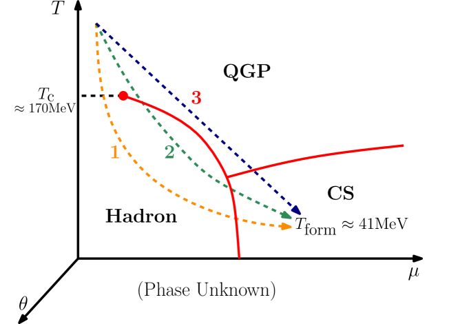
The main goal of the present work is to present robust arguments (supported by the detail analytical and numerical computations) that a sufficiently strong global $\cal{CP}$ violation in form of the fundamental axion field $\theta(x)$ inevitably leads to such separation of baryon charges. This phenomena of separation is preceding the QCD transition. As we argue in the present work this axion $\theta(x)$ field can be thought as the Berry’s phase which is coherently accumulated on the largest possible scales of the visible Universe. Precisely this coherence leads to a preferential evolution of the nuggets when one type of the visible baryons (not anti- baryons) prevails in the system. This source of strong $\cal CP$ violation is no longer available at the present epoch as a result of the axion dynamics, see original papers [6, 7, 8], recent reviews [9, 10, 11, 12, 13, 14, 15, 16] and recent results/proposals on the axion search experiments [19, 17, 18, 20, 21, 22, 23, 24, 25, 26, 27, 28, 29].

The basic consequence of this framework is that the visible and dark matter densities are of the same order of magnitude [4]:

$$\Omega_{\rm dark}\approx\Omega_{\rm visible}.$$ (1)

This is a very generic consequence of the entire framework, and it is not sensitive to the parameters of the system, such as the axion mass $m_{a}$. In our framework the relation (1) emerges in a very natural way because both types of matter (visible and dark) are proportional to a single dimensional parameter of the system, $\Lambda_{\rm QCD}$.

The very generic relation (1) of this framework is also not sensitive to the initial value $\theta_{0}$ of the coherent axion field when it starts to oscillate. This should be contrasted with conventional mechanisms (such as production of the axions due to the misalignment mechanism or due to the domain wall network decay) which are highly sensitive to these parameters as $\Omega_{\rm axion}\sim\theta^{2}_{0}m_{a}^{-7/6}$, see reviews [9, 10, 11, 12, 13, 14, 15, 16].

In particular, the observed ratio $\Omega_{\rm dark}\simeq 5\cdot\Omega_{\rm visible}$ would correspond to a slight asymmetric excess of anti-nuggets comparing to the nuggets by a factor of $\sim 0.5$ at the end of the nugget’s formation, if one assumes that the nuggets saturate the dark matter density today. Thus, the approximate observed ratio $\Omega_{\rm dark}\simeq 5\cdot\Omega_{\rm visible}$ roughly corresponds to

$$|B_{\rm visible}|:|B_{\rm nuggets}|:|B_{\rm antinuggets}|\simeq 1:2:3,$$ (2)

such that the net baryonic charge is zero.

The quark nuggets at zero temperature satisfy the main criteria to be the DM candidates as they are absolutely stable configurations made of quarks and gluons surrounded by the axion domain wall as described in the original paper [1]. However, unlike conventional dark matter candidates, such as WIMPs, the dark-matter/antimatter nuggets are macroscopically large objects and they strongly interact with visible matter. The quark nuggets do not contradict the observational constraints on dark matter or antimatter for three main reasons [34]:

• They carry very large baryon charge $|B|\gtrsim 10^{25}$, and so their number density is very small $\sim B^{-1}$. As a result of this unique feature, their interaction with visible matter is highly inefficient, and therefore, the nuggets are perfectly qualify as DM candidates. In particular, the quark nuggets essentially decouple from CMB photons, and therefore, they do not destroy conventional picture for the structure formation;

• The core of the nuggets have nuclear densities. Therefore, the relevant effective interaction is very small $\sigma/M\sim 10^{-10}$  cm²/g. Numerically, it is comparable with conventional WIMPs values. Therefore, it is consistent with the typical astrophysical and cosmological constraints which are normally represented as $\sigma/M<1$ cm²/g;

• The quark nuggets have very large binding energy due to the large gap $\Delta\sim 100$ MeV in superconducting phases. Therefore, the baryon charge is so strongly bounded in the core of the nugget that it is not available to participate in big bang nucleosynthesis (bbn) at $T\approx 1$ MeV, long after the nuggets had been formed.

We emphasize that the weakness of the visible-dark matter interaction in this model is due to a small geometrical parameter $\sigma/M\sim B^{-1/3}$ which replaces the conventional requirement of sufficiently weak interactions for WIMPs.

Figure 1: The conjectured phase diagram. The plot is taken from [4]. Possible cooling paths are denoted as path 1, 2 or 3. The phase diagram is in fact much more complicated as the dependence on the third essential parameter, the $\theta$ is not shown as it is largely unknown. It is assumed that the final destination of the nuggets is the CS region with $T_{\rm form}\approx 41$ MeV, $\mu>\mu_{c}$ and $\theta\approx 0$.

We conclude this Introduction with the following remark. We consider the model which has a single fundamental parameter (the mean baryon number of a nugget $\langle B\rangle\sim 10^{25}$, corresponding to the axion mass $m_{a}\simeq 10^{-4}~{}\rm eV$). It has been shown that this model is consistent with all known observations, including the satellite and ground based constraints. It has been also shown that there is a number of frequency bands where some excess of emission was observed, and this model may explain some portion, or even entire excess of the observed radiation in these frequency bands. We refer to recent short review [35] with large number of references on original computations which have been carried out for each specific frequency band where some excess of radiation has been observed.

The paper is organized as follows. In Section II we overview the big picture of our framework when the “baryogenesis” is replaced by the baryon charge separation scenario, and the DM is represented by quark nuggets and anti-nuggets. We list the crucial ingredients of the entire framework by paying special attention to the role the coherent $\cal{CP}$-odd axion field discussed in details in subsection II.5.

Essentially, the main objective of the present work is to elaborate on this specific key element of the proposal which has not received sufficient attention in the previous paper [4]. Our goal of this work is to present solid quantitative computations suggesting that this coherent $\cal{CP}$-odd axion field generates the disparity between nuggets and anti-nuggets. This asymmetry automatically leads to the relation (1) which we claim is very generic consequence of the entire framework.

The readers who are not interested in any technical details may skip the next two sections (III and IV) and jump directly to the concluding section V.

In Section III we argue that the nuggets and anti-nuggets behave in a drastically different way as a result of interaction with this $\cal{CP}$-odd coherent cosmological axion field. Finally, in section IV we argue that the difference in evolution of the nuggets and anti-nuggets is always of order of one effect, being insensitive to initial conditions nor to the dynamical parameters of the system. As a result, the main claim of this proposal represented by eq.(1) is very robust consequence of the framework and is not a result of any fine tuning adjustments.

II Big picture and the crucial elements of the proposal

In this section we summarize the crucial elements of the proposal which describe the formation of the nuggets. These ingredients determine the basic properties of the nuggets, such as the size, local accretion of baryonic charge, abundance, stability, and global $\cal CP$ violating charge separation leading to the disparity between nuggets and anti-nuggets. Most of these basic elements of the proposal have been discussed previously in the original papers [1] and [4]. We include them into the present work to make it self-contained. One crucial ingredient of the proposal which was mentioned in [4] but has not been fully elaborated there is related to the $\cal CP$ violating processes leading to the asymmetry between nuggets and anti-nuggets. We highlight the basic idea on $\cal CP$ violation in subsection II.5, while the detail analysis of this ingredient of the proposal is carried out in “technical” sections III and IV.

II.1 $N_{\rm DW}=1$ domain walls

The first important element, axion domain wall [36, 37], determines the size of a nugget as originally suggested in [1]. The axion field $\theta$ is an angular variable, and therefore supports various types of the topological domain walls (DW), including the so-called $N_{\rm DW}=1$ domain walls when $\theta$ interpolates between one and the same physical vacuum state with the same energy $\theta\rightarrow\theta+2\pi n$.

It is important to emphasize that while the axion string formation happens during the Peccei-Quinn (PQ) phase transition, the domain wall formation occurs at the QCD temperature at $T\sim 1$ GeV when the axion potential gets tilted. In other words, the formation of the DW-string network is the two stages process, rather than a single event, see [37] for review. Furthermore, the DW energy density per unit volume is characterized by a typical QCD scale, rather than the PQ scale. Therefore, the closed DW surfaces, without attached strings, could be formed during the QCD transition, though the number density of such objects is suppressed with increasing the size of the objects [37, 38], see subsection II.3 with few more comments and estimates on this suppression.

One should also add that the numerical simulations [38] support this picture by observing the formation of the large DW at the QCD temperature and their decay due to the attached strings. The closed DW without attached strings have been also observed in numerical simulations [37, 38], though the probability to find the closed walls is suppressed according to (4). Due to this suppression, the role of these closed DW is normally ignored in the analysis of the DW decays to the DM axions. However, precisely these closed DW surfaces formed at the QCD scale play the key role in our proposal [1], see additional comments at the end of this subsection.

One should remark here that it is normally assumed that for the topological defects to be formed, the PQ phase transition must occur after inflation. This argument is valid for a generic type of domain walls with $N_{DW}\neq 1$. The conventional argument is based on the fact that few physically different vacua with the same energy must be present inside of the same horizon for the domain walls to be formed. The $N_{DW}=1$ domain walls are unique and very special in the sense that $\theta$ interpolates between one and the same physical vacuum state. Such $N_{DW}=1$ domain walls can be formed even if the PQ phase transition occurred before inflation and a unique physical vacuum occupies entire Universe [4].

In other words, while in our proposal the inflation is assumed to occur after the PQ phase transition and the axion field $\theta(t)$ is coherent in the entire visible Universe, nevertheless the $N_{DW}=1$ closed domain walls can still be formed. The nonzero $\theta$ would essentially lead to a global $\cal CP$ violating separation of baryonic charge as discussed in item II.5.

The axion domain walls normally start to form once the axion field get tilted at temperature $T_{a}$. As the tilt becomes more pronounced (at the transition when the chiral condensate forms at $T_{c}$) the DW formation becomes much more efficient. We should expect, in general, that the $N_{\rm DW}=1$ domain walls form at any moment between $T_{a}$ and $T_{c}$. The width of the domain wall depends on the mass of the axion, which would ultimately determine the size of the nugget being formed.

One next comment is as follows. It has been realized many years after the original publication [36] that the axion domain walls generically demonstrate a sandwich-like substructure on the QCD scale $\Lambda_{\rm QCD}^{-1}\simeq\rm fm$. Such a substructure is supported by analysis [39] of QCD in the large $N$ limit with inclusion of the $\eta^{\prime}$ field. It is also supported by analysis [40] of supersymmetric models where a similar $\theta$ vacuum structure occurs. The same structure also occurs in colour superconducting (CS) phase where the corresponding domain walls have been explicitly constructed [41].

Significance of the QCD substructure is that it is capable to squeeze the quarks to bring the system into the CS state, as originally suggested in [1]. The fact that the CS phase representing the lowest energy state might be realized in nature in the core of neutron stars has been known for quite sometime. A less known application of the CS phase is that the axion DW with the QCD substructure may replace the gravity and play the role of a squeezer to produce an absolutely stable quark nugget at $T=0$ as suggested in [1].

The time evolution of these nuggets at $T\neq 0$ is much more involved problem than the study of the equilibrium configurations at $T=0$ carried out in [1]. The corresponding problem of the time evolution at $T\neq 0$ has been recently addressed in [4]. In particular, in that paper it has been shown that the nuggets assume the equilibrium at low temperature with the lowest possible state if the initial size of the nugget is sufficiently large. These results fully support the earlier studies of ref.[1] devoted to the equilibrium configurations at $T=0$.

To conclude this subsection. The formation of the axion DW at the QCD transition is extremely generic phenomenon which inevitably occurs as a result of $\theta\rightarrow\theta+2\pi n$ periodicity. These axion DW typically have the QCD substructure as mentioned above. Furthermore, the formation of the closed surfaces at the QCD transition (which eventually may produce the quark nuggets) also represents a very generic feature of the system, which will be further elaborated in subsection II.3.

II.2 Spontaneous breaking of $\cal{C}$ symmetry on small scale of order $\xi(T)$

The second important element of the formation mechanism can be explained as follows. There is another substructure with a similar QCD scale (in addition to the known substructures expressed in terms of the $\eta^{\prime}$ and gluon fields as explained in section II.1 above) which carries the baryon charge. This additional substructure is a novel feature of the axion domain walls which has been explored only recently in [4]. As (anti)quarks being trapped in the core of the domain wall, the nuggets itself slowly accrete the baryonic charge as a result of evolution. Exactly this new effect is eventually responsible for local accretion of the baryonic charge by the nugget.

Indeed, in the background of the domain wall, the physics essentially depends on two variables, $(t,z)$. One can show that in this circumstances the total baryon charge $B$ accumulated on a nugget is determined by the degeneracy factor in vicinity of the domain wall [4]

$$B=N\cdot g\cdot\int\frac{d^{2}x_{\perp}d^{2}k_{\perp}}{(2\pi)^{2}}\frac{1}{\exp(\frac{\epsilon-\mu}{T})+1}.$$ (3)

In this formula the induced baryon number $N$ per degree of freedom may randomly assumed any integer value, positive or negative; the coefficient $g$ describes the degeneracy factor, e.g. $g\simeq N_{c}N_{f}$ in CS phase and $\mu$ is the chemical potential in the vicinity of the domain wall. Thus, the size distribution for quark and antiquark nuggets will be identically the same size if the external environment is $\cal CP$ even, which is the case when fundamental $\theta=0$.

The crucial element here is that the domain walls will acquire the baryon or anti-baryon charge as a generic feature of the system. This is because the domain wall tension is mainly determined by the axion field while the QCD substructure leads to small correction factor of order $\sim\Lambda_{\rm QCD}/f_{a}\ll 1$. Therefore, the presence of the QCD substructure with nonvanishing $N\neq 0$ increases the domain wall tension only slightly. Consequently, this implies that the domain wall closed bubbles carrying the baryon or antibaryon charge will be copiously produced during the transition as they are very generic configurations of the system. Furthermore, the baryonic charge cannot leave the system during the time evolution as it is strongly bound to the wall due to the topological reasons. The corresponding binding energy per quark is order of $\mu$ and increases with time as shown in [4]. One can interpret this phenomenon as a local spontaneous breaking of $\cal{C}$ symmetry, when on the scales of order the correlation length $\xi(T)\sim m_{a}^{-1}(T)$, the nuggets may acquire the positive or negative chemical potential $\mu$ with equal probability. This is because the sign of $N$ in Eq. (3) may assume any positive or negative values with equal probabilities.

II.3 Kibble-Zurek mechanism

The Kibble-Zurek (KZ) mechanism gives a generic picture of formation of the topological defects during a phase transition. We refer to the original papers [42], review [43] and the textbook [37] for a general overview. For our specific purposes of the DW formation, the KZ mechanism suggests that once the axion potential is sufficiently tilted the $N_{\rm DW}=1$ closed domain walls form at the QCD scale. Some time after $T_{a}$ the system is dominated by a single, percolated, highly folded and crumple domain wall network of very complicated topology. In addition, there will be a finite portion of the closed walls (bubbles) with typical size of order correlation length $\xi(T)$, which is defined as an average distance between folded domain walls at temperature $T$. Parametrically, the correlation length $\xi(T)\sim m^{-1}_{a}(T)$ is determined by the axion mass, and obviously varies with time during the network evolution. Precisely these bubbles are capable to form the nuggets and play the crucial role in our analysis. It is known that the probability $n$ of finding closed walls with very large size $R\gg\xi$ is exponentially small, see [37] for review,

$$n\sim\exp{\left[-\frac{R^{2}}{\xi^{2}(T)}\right]}.$$ (4)

The key point for our proposal is mere existence of these finite closed bubbles made of the axion domain walls. Normally it is assumed that these closed bubbles collapse as a result of the domain wall pressure, and do not play any significant role in dynamics of the system because the total area of these bubbles is sufficiently small in comparison with the area of the dominant percolated domain wall network. However, as we already mentioned in section II.1 some of these closed bubbles do not collapse due to the Fermi pressure acting inside of the bubbles. The equilibrium is achieved when the Fermi pressure from inside due to the degenerate quarks equals to the pressure from outside due to the axion domain wall. This is precisely the condition of the stability analyzed in ref. [1].

There are many papers devoted to analysis of the network made of the domain walls bounded by the strings. There are also many papers devoted to the problem (and its possible resolutions) on the domain wall dominance of the Universe. We have nothing new to add to these subjects and we refer to the original literature [38, 44, 45, 46, 47] and reviews [37, 11] on this matter. Those axions (along with the axions produced by the conventional misalignment mechanism [44, 48]) will contribute to the dark matter density today. The corresponding contribution to DM density is highly sensitive to the axion mass as $\Omega_{\rm dark}\sim m_{a}^{-7/6}$, and it is not part of our framework.

Instead, our proposal focuses on the dynamics of the closed bubbles (4), which are formed during the QCD transition. These closed bubbles are normally ignored in computations of the axion production. Precisely these closed bubbles will eventually become absolutely stable quark nuggets and may serve as the dark matter candidates according to the proposal [1, 4].

The efficiency of the production of these bubbles has been estimated in ref.[4], based on assumption that this mechanism saturates the observed ratio $n_{B}/n_{\gamma}\sim 10^{-10}$. We shall not discuss this model-dependent estimate in the present work as the main goal of the present analysis is to demonstrate that $c(T)\sim 1$ in eq. (8).

II.4 Colour Superconductivity

The existence of CS phase in QCD is the crucial element for the stability of quark nuggets. In astrophysics, a CS is known to be the plausible phase in the neutron star interiors and in the violent events associated with collapse of massive stars or collision of neutron star, see review papers [49, 50] on the subject. The CS phase becomes energetically favourable when quarks are squeezed to few times of nuclear density.

Analogous to the gravitational squeezing in neutron star, the CS phase might be realized in quark nuggets due to the surface tension of the axion domain wall as advocated in [1]. The domain wall bubbles after formation will undergo a large number of bounces with typical frequency $\omega\sim m_{a}$ until they settle down at the equilibrium configuration [4]. As the temperature cools down, the oscillations and squeezing will turn the bulk of quarks into an equilibrium position with ground state being in the CS phase.

The corresponding time evolution of an oscillating bubble can be approximated as follows:

$$R(t)=R_{\rm form}+(R_{0}-R_{\rm form})e^{-t/\tau}\cos\omega t,$$ (5)

where the initial radius of a bubble $R_{0}\sim\xi(T)$ is assumed to be of order the correlation length $\xi(T)$. The final size $R_{\rm form}$ of a bubble represents the equilibrium configuration when formation is almost complete. In formula (5) parameter $\tau$ represents a typical damping time scale which is expressed in terms of the axion mass $m_{a}$, and the QCD parameters such as viscosity. It turns out the numerical value of $\tau$ is of order of the cosmological scale $\tau\sim 10^{-4}\rm s$. This numerical value is fully consistent with our anticipation that the temperature of the Universe drops approximately by a factor of $\sim 3$ or so during the formation period. During the same period of time the chemical potential $\mu$ inside the nugget reaches sufficiently large value when the CS phase sets in [4].

II.5 Coherent $\cal{CP}$-odd axion field

The key element to be investigated in the present work, is the $\cal CP$ asymmetric charge separation originating from the globally coherent axion field $\theta(t)$. In this subsection we outline the basic ideas while all technical details will be elaborated in sections III and IV.

It is well known that the axion dynamics at sufficiently large temperature $T>T_{c}$ is determined by the coherent state of axions at rest, see e.g. review paper [11]:

$$\theta(t)\sim\frac{C}{t^{3/4}}\cos\int^{t}dt^{\prime}\omega_{a}(t^{\prime}),~{}\omega_{a}^{2}(t)=m_{a}^{2}(t)+\frac{3}{16t^{2}},~{}~{}~{}~{}$$ (6)

where $C$ is a constant, and $t=\frac{1}{2H}$ is the cosmic time. This formula describes the dynamics of the axion field after the moment $t_{1}$ determined by the condition $m_{a}(t_{1})t_{1}=1$ when the axion mass $m_{a}$ effectively turns on at $t_{1}$. Precisely this moment is relevant for our studies as the domain walls start to form after $t_{1}$. For sufficiently large $t$ when $m_{a}(t)t\gg 1$ the second term in expression for $\omega_{a}^{2}(t)$ can be ignored and the frequency of the oscillations $\omega_{a}(t)$ is determined by the axion mass at time $t$,

$$\dot{\theta}(t)\sim\omega_{a}(t)\simeq m_{a}(t).$$ (7)

The key point in what follows is the observation that $\theta(t)$ is one and the same in the entire visible Universe. One should also emphasize that this assumption on coherency of the axion field on very large scales is consistent with formation of $N_{\rm DW}=1$ domain walls as explained in subsection II.1.

Similar to the case of formation temperature $T_{\rm form}$ discussed in details in [4], precise dynamical computation of this $\cal CP$ asymmetry due to the coherent axion field $\theta(t)$ is a hard problem of strongly coupled QCD at $\theta\neq 0$ when even the phase diagram, schematically shown on Fig.1 is not yet known. It depends on a number of specific properties of the nuggets, their evolution, their environment, modification of the hadron spectrum at $\theta\neq 0$ and corresponding cross sections as mentioned in [4]. All these factors equally contribute to the difference between the nuggets and anti-nuggets. One can effectively account for these coherent $\cal CP$ odd effects by introducing an unknown coefficient $c(T)$ of order one as follows [4]

$$B_{\rm antinuggets}=c(T)\cdot B_{\rm nuggets},~{}~{}{\rm where}~{}~{}|c(T)|\sim 1.~{}~{}$$ (8)

The main goal of the present work is to provide the quantitative numerical analysis supporting the basic assumption (8). We shall argue that $|c(T)|\sim 1$ is indeed very likely to be of order of one as a result of the $\cal CP$ violating processes which took place coherently on enormous scale of the entire visible Universe before the QCD transition. We shall argue below that this very generic outcome of this framework is not very sensitive to initial conditions (such as the magnitude of $\theta_{0}$ at the moment of formation), nor to a precise value of the axion mass $m_{a}(T)$ at $T>T_{c}$ when the domain wall network only started to form. The fundamental ration (1) is the direct consequence of $|c(T)|\sim 1$. Therefore the arguments supporting (8) are essentially equivalent to the basic claim of this framework (1).

What is the significance of eq. (8)? The most important and unambiguous consequence of the eq. (8) is that the baryon charge in form of the visible matter can be also expressed in terms of the same coefficient $c(T)\sim 1$ as follows $B_{\rm visible}=-(B_{\rm antinuggets}+B_{\rm nuggets})$. Using eq. (8) the expression for the visible matter $B_{\rm visible}$ can be rewritten as [4]

$$B_{\rm visible}\equiv\left(B_{\rm baryons}+B_{\rm antibaryons}\right)$$ (9)

$$=-\left[1+c(T)\right]B_{\rm nuggets}=-\left[1+\frac{1}{c(T)}\right]B_{\rm antinuggets}.$$

This is very important relation which we would like to represent in terms of the measured observables $\Omega_{\rm visible}$ and $\Omega_{\rm dark}$ at late times when the visible matter consists the baryons only [4]:

$$\Omega_{\rm dark}\simeq\left(\frac{1+|c(T)|}{\left|1+c(T)\right|}\right)\cdot\Omega_{\rm visible}~{}~{}{\rm at}~{}~{}T\leq T_{\rm form}.$$ (10)

Important comment here is that the relation (9) holds as long as the thermal equilibrium is maintained. Furthermore, the thermal equilibrium implies that each individual contribution $|B_{\rm baryons}|\sim|B_{\rm antibaryons}|$ entering (9) is many orders of magnitude greater than the baryon charge hidden in the form of the nuggets and anti-nuggets at earlier times when $T_{c}>T>T_{\rm form}$. However, the net baryon charge which is labeled as $B_{\rm visible}$ in eq. (9) is the same order of magnitude as the net baryon charge hidden in the form of the nuggets and anti-nuggets.

For a specific value of $c(T_{\rm form})\simeq-1.5$ the relations (9) and (10) assume the form

$$B_{\rm visible} \simeq \frac{1}{2}B_{\rm nuggets}\simeq-\frac{1}{3}B_{\rm antinuggets},$$

$$\Omega_{\rm dark} \simeq 5\cdot\Omega_{\rm visible}.$$ (11)

These numerical values coincide with approximate relation (2) presented in Introduction. The coefficient $\sim 5$ in relation $\Omega_{\rm dark}\simeq 5\cdot\Omega_{\rm visible}$ is obviously not universal, but relation (10) is universal, and very generic consequence of the entire framework, which was the main motivation for the proposal [1, 2].

We shall argue in next sections III and IV that $|c(T)|\sim 1$ is indeed of order of one. Furthermore, we shall argue this feature of the system is universal, and not very sensitive to the axion mass $m_{a}(T)$ nor to the initial value of $\theta_{0}$ when the bubbles start to oscillate and slowly accrete the baryon charge. The only crucial factor in our arguments is that the axion field $\theta(t)$ can be represented by the coherent superposition of the axions at rest (6).

III Evolution of the (anti) nuggets in the background of the axion field

In this section, we study the profound consequences of the coherent axion phase on the nugget’s formation. Essentially, the main goal of this section is to present analytical and numerical arguments suggesting that small $\mathcal{CP}$ violating effects will produce a large disparity (of order of one) between the nuggets and anti-nuggets.

We start with subsection III.1 where we present some qualitative explanation of how a relatively small fundamental coupling between quarks/antiquarks and the coherent axion $\theta(t)$ field given by (6) may, nevertheless, produce a large asymmetry in properties between the nuggets and anti-nuggets. In following subsections III.2 and III.3 we develop the technical tools to address these questions, while in subsection III.4 we present our estimates supporting the main claim of this work that $|c(T)|\sim 1$.

III.1 Qualitative analysis

Before we start our specific quantitative studies in this section we want to formulate few generic relations which characterize the system and which depend exclusively on symmetric features of the system, rather than on some specific dynamical model-dependent computations which follow.

First of all, let us remind that if $\langle\theta\rangle=0$ the baryon charge hidden in nuggets on average is equal to the baryon charge hidden in anti-nuggets, of course with sign minus. Indeed, the studies of the anti-nuggets can be achieved by flipping the sign of the chemical potential $\mu\rightarrow-\mu$ in analysis of ref. [4]. One can restore the original form of the effective Lagrangian by flipping the sign for the axion $\theta$ field as discussed in [4]. These symmetry arguments imply that as long as the pseudo-scalar axion field $\theta$ fluctuates around zero $\langle\theta\rangle=0$ as conventional pseudo-scalar fields (such as $\pi,\eta^{\prime}$ mesons, for example), the theory remains invariant under $\cal{P}$ and $\cal{CP}$ symmetries and on average an equal number of nuggets and anti-nuggets carrying equal baryon (anti-baryon) charges would form.

However, if $\langle\theta\rangle\neq 0$ there are many strong processes taking place inside and outside the nuggets (such as annihilation, evaporation, scattering, etc) which are slightly different for nuggets and anti-nuggets, as reviewed in in Appendix A. Furthermore, the vacuum energy itself and the density of states in all these regions are also slightly different because the vacuum condensate (38) assumes slightly different numerical values in all these regions as it depends on $\mu,T$ and $\theta$.

Precise computations of all these coherent $\cal{CP}-$ violating QCD effects are hard to carry out explicitly as they require solution of many body effects in unfriendly environment with non-vanishing $\theta,\mu,T$ when even the phase diagram is not yet known, see Fig. 1. However, the estimation of the effect is very simple exercise as it must be proportional to $\theta(t)$ at the moment when the domain walls start to form. Numerically, this parameter $|\theta(t)/\theta_{0}|\sim 10^{-2}-10^{-3}$ could be quite small, and naively may lead only to minor effects $\leq 10^{-2}$. However, the crucial point here is that while this coupling is indeed small on the QCD scale, it nevertheless effectively long-ranged and long lasting, in contrast with conventional random QCD processes. As a result, these coherent $\cal{CP}-$ violating effects will produce large effects of order one as explicit computations carried out below show.

The crucial element in making such assessment is the observation that these small coherent changes occur in the entire volume of a nugget. In other words, the generation of the chemical potential, accumulation the phase difference (which eventually leads to the accretion of the baryon charge) etc are proportional to the volume of the nugget,

$$\Delta B\sim\theta(t)V,~{}~{}~{}~{}|\theta(t)/\theta_{0}|\sim 10^{-2}-10^{-3},$$ (12)

where $\Delta B$ is the baryon charge difference in accumulation between the nuggets and anti-nuggets. This expression should be contrasted with effect due to the local spontaneous violation of the $\cal{C}$-symmetry (as discussed in [4] and reviewed in section II.2) which is proportional to the surface of a nugget, $B\sim S$, see eq.(3).

While all individual events are proportional to small parameter $\theta\ll 1$, and therefore, numerically small, this difference (between a typical size for nuggets vs anti-nuggets) eventually will be order of one as a result of long lasting evolution, as is shown in next subsections. This strong effect of order of one has been phenomenologically accounted for by parameter $c(T)$ in formula (8), which automatically leads to the main consequence of this framework expressed by relation (1).

III.2 Basic equations

We start with brief overview of the work [4], where it was assumed that the $\cal CP$ symmetry is globally conserved, i.e. $\langle\theta(t)\rangle=0$ when average over entire Universe. In that paper the effective interaction of the axion domain wall with Fermi fields was approximated as follows

$$\mathcal{L}_{4}=\bar{\Psi}(i\not{\partial}-me^{i[\theta(x)-\phi(x)]\gamma_{5}}-\mu\hat{\gamma}_{0})\Psi,$$ (13)

where parameter $m$ should not be interpreted as the quark’s mass. Rather, it is much more appropriate to interpret parameter $m$ as the expectation value of the $\langle{\rm det}~{}\bar{\psi}_{L}^{f}\psi_{R}^{f}\rangle$ from eq (38) which has a typical QCD scale and which will be always generated even in deconfined regime at $T>T_{c}$. The Fermi field $\Psi$ should be interpreted as the low-energy (soft) component of the original quark fields, while a high energy component has been integrated out to generate parameter $m$ entering (13). The equation (13) is the standard form for the interaction between the pseudo-scalar fields (axion $\theta(x)$ and $\eta^{\prime}$ field parametrized by $\phi(x)$) and the fermions (quarks and antiquarks) which respect all relevant symmetries in presence of nonzero chemical potential $\mu$.

Another key element from [4] which is relevant for our present studies is the effective Lagrangian describing the dynamics of an oscillating domain wall bubble

$$L = \frac{4\pi\sigma R^{2}(t)}{2}\dot{R}^{2}(t)-4\pi\sigma R^{2}(t)$$

$$+ \frac{4\pi R^{3}(t)}{3}\Delta P(\mu)+\left[{\rm other~{}terms}\right].$$

The equation (III.2) describes the time evolution of the closed spherically symmetric domain wall bubble of radius $R(t)$. The pressure term $\Delta P=P^{\rm(Fermi)}+P^{\rm(Bag)}-P^{\rm(out)}$ in eq. (III.2) can be parametrized as [4]

$$\Delta P=\frac{g^{\rm in}T^{4}}{6\pi^{2}}I_{4}(b)-E_{B}\theta(b-b_{1})\left(1-\frac{b_{1}^{2}}{b^{2}}\right)-\frac{\pi^{2}g^{\rm out}T^{4}}{90},$$

where $g^{\rm in}\simeq 2N_{c}N_{f}$ and $g^{\rm out}\simeq\left(\frac{7}{8}4N_{c}N_{f}+2(N_{c}^{2}-1)\right)$ are degeneracy factors for inside and outside of the bubble respectively; $b=|\mu|/T$ is the dimensionless parameter to be used frequently in what follows; $I_{4}(b)$ is a specific type of Fermi integrals, see Appendix E; finally $E_{B}\sim(150~{}{\rm MeV})^{4}$ is the famous “bag constant” from the MIT bag model, which turns on in the hadronic phase at small $\mu<\mu_{1}$, while it vanishes in CS phase at large $\mu>\mu_{1}$.

The evolution of the bubble is governed by the following differential equations [4]

$$\frac{d}{dt}B_{\rm wall}=0,~{}~{}~{}~{}B_{\rm wall}=\frac{g^{\rm in}ST^{2}}{2\pi}I_{2}(b)$$ (15a)

$$\sigma\ddot{R}=-\frac{2\sigma}{R}-\frac{\sigma\dot{R}^{2}}{R}+\Delta P(b)-4\eta\frac{\dot{R}}{R}.$$ (15b)

where $\sigma\simeq 9f_{a}^{2}m_{a}$ is the domain wall tension, while $\eta\simeq m_{\pi}^{3}$ is the QCD viscosity. The baryonic charge for nuggets can be expressed in terms of the Fermi integral $I_{2}(b)$ given in Appendix E. Eq. (15a) describes an implicit dependence of chemical potential on size of the nugget, $\mu(R)$. It should be substituted to eq. (15b) to arrive to the differential equation which describes the time evolution of the nugget $R(t)$. The corresponding analysis has been performed in [4] with the basic result that the solution can be well approximated by slow damping oscillations with typical frequency $m_{a}$ around $R_{\rm form}$ as presented by eq. (5).

As we already mentioned, in the preceding studies [4] on the bubble evolution we had assumed that the $\cal CP$-symmetry is conserved as no interaction with the coherent axion field $\theta(t)$ was included into the consideration. Now we wish to include the coherent axion field $\theta(t)$, given by eq.(6) into the equations. The most important change which occurs as a result of the interaction of the Fermi fields with the background axion field is the accumulation of the phase (36) as a result of the coupling $\Psi$ field with axion field $\theta(t)$, which can be interpreted as the coherent Berry’s phase, as explained in Appendix A.

To proceed with the computations one could follow the procedure developed in [4], rewrite the Fermi fields in 2d notations (accounting for the domain wall background) and represent the extra term to the effective Lagrangian due to the coupling with external axion field as follows

$$\Delta\mathcal{S} = -\frac{1}{\pi}\int dz\mu(z)\partial_{z}\theta(t),$$ (16)

$$A \equiv -\frac{\delta\Delta\mathcal{S}}{\delta\mu}=\frac{1}{\pi}\int_{R_{\rm in}}^{R_{\rm out}}dz\cdot\left(\frac{\partial\theta}{\partial t}\right)\frac{1}{\dot{R}},$$

where the end points of the integral $z=(R_{\rm in},R_{\rm out})$ should be interpreted as the typical distances describing the regions inside and outside the bubble of a typical size $z\simeq R$.

Few comments are in order. First, one can explicitly see from eq. (16) that the effect is different for nuggets and anti-nuggets as the sign of $\mu$ is opposite in these cases, while the background field $\theta(t)$ remains the same in entire visible Universe. Secondly, parameter $A$ can be interpreted as an additional baryon charge (per degree of freedom) accumulated by a nugget during a single nugget’s cycle. This coefficient can be approximated as follows

$$A\simeq\frac{\Delta\theta}{\pi},$$ (17)

where $\Delta\theta$ can be interpreted as the variation of the axion field during a single-nugget’s cycle. One should emphasize that the correction (17) is not the only source leading to the disparity between nuggets and anti-nuggets. In fact many other $\cal{CP}$ violating processes may also contribute to the differences in accumulating baryon charges for nuggets and anti nuggets. We expect that all these effects mentioned in footnote 4 are equally important as they must be proportional to the $\cal{CP}$ violating parameter $\theta(t)$. Therefore, the corresponding effects may be effectively accounted for by a modification of the numerical coefficient $A$ entering (17). As we argue below, the outcome of the calculations is not very sensitive to a specific value of coefficient $A$. Therefore, neglecting a large number of different $\cal{CP}$ violating processes mentioned in footnote 4 (which can be accounted for by modifying the numerical coefficient $A$) does not affect the main result of our analysis.

Our next remark is the observation that the phase (6) and corresponding extra energy (16) is accumulated coherently by large portion of quarks inside of a nugget of volume $V$, while corresponding correction to the vacuum energy obviously vanishes outside the nuggets where $\mu\simeq 0$. To compute the correction to the baryon charge of a nugget due the coupling to the axion $\theta$ field one should multiply (17) to the degeneracy factor, i.e.

$$B_{\theta}^{(\pm)} = \pm g^{\rm in}AV\int\frac{d^{3}k}{(2\pi)^{3}}\frac{1}{\exp(\frac{k}{T}-b)+1}$$

$$= \pm\left(\frac{g^{\rm in}ST^{2}}{2\pi}I^{(\pm)}_{2}(b)\right)\cdot\left(\frac{ART}{3\pi}\frac{I^{(\pm)}_{3}(b)}{I^{(\pm)}_{2}(b)}\right),$$

where we assume that the chemical equilibration is sufficiently fast such that one can use one and the same $\mu$ within entire volume of the nugget. Furthermore, in writing down equation (III.2) we assumed that the majority of quarks in volume $V$ move coherently during the bubble oscillations. In fact, the coherence might not be so perfect, and only some portion of the quarks inside the nuggets might move coherently as a macroscopical system. It is very hard to estimate the corresponding suppression factor within our framework formulated in terms of a single macroscopical variable $R(t)$. The corresponding suppression factor may be effectively accounted for by some modification of the numerical coefficient $A$ entering (III.2). As we already previously mentioned our results are not very sensitive to an absolute value of numerical value of $A$ as long as it is not exceedingly small. Therefore, we assume that all correction factors mentioned previously in footnote 4 and suppression factor due to not perfect coherent motion are implicitly included in coefficient $A$ in analysis which follows.

Our next remark goes as follows. In eq. (III.2) we presented the expression for $B^{(\pm)}_{\theta}$ as a combination of two factors. The first factor is precisely the expression for the baryon charge $B_{\rm wall}$ from eq. (15a) generated spontaneously as described in [4]. The second factor represents the correction to the accumulated baryon charge due to the coupling of the $\cal CP$ odd axion field with quarks inside the nugget. It is important to emphasize that it is numerically suppressed due to small $\cal CP$ violating phase (6) parametrized by small numerical coefficient $A$. However, it is strongly enhanced by large numerical factor proportional to the size of the system. In contrast to the baryon accumulation in Eq. (15a) which is proportional to the surface, the $B_{\theta}^{(\pm)}$ contribution is proportional to the volume of the system (III.2), in agreement with qualitative arguments (12) of the previous section.

Our next comment is as follows. Naively, one could think that the accumulation of the baryon charge by a nugget due to the coherent interaction with the axion field $\theta$ will be very fast since it is proportional to the volume $V$ of the nugget according to (III.2). However, the accumulation is in fact quite slow. The point is that the axion $\theta$ field oscillates with time, $\sim\cos(m_{a}t)$ and the accumulated baryon charge is almost washed out during a complete cycle of the axion $\theta(t)$ field. Nevertheless, the cancellation is not quite complete because the axion field slowly reduces its amplitude. The main reason for this amplitude’s decay is the emission of real physical axions (due to misalignment mechanism) which is the source of some non- equilibrium dynamics. Precisely this slow decrease of the axion amplitude leads to a non-vanishing $\Delta\theta$ entering (17), and eventually generates the disparity between nuggets and anti-nuggets.

Recapitulate: a tiny portion of the accumulated baryon charge remains in the nuggets after every single complete cycle such that the disparity between nuggets and anti-nuggets will be accumulated but at very slow pace as a result of very large number of oscillations. Based on this fact, we can therefore assume $A$ as an adiabatic “constant” for each given cycle in the analysis in following subsections III.3 and III.4.

Our final remark regarding eq. (III.2) is as follows. This formula was derived by considering the coherently moving quarks of the nuggets in the background of the axion field (6). This approximation is only justified as long as the effect due to the background field is sufficiently small. Formally, the effect (III.2) due to the axion field must be much smaller than the initial accumulation of the baryon charge (15a) due to the spontaneous local symmetry breaking when the original chemical potential $\mu$ is generated. Such a condition must be imposed on our system to avoid any complications related to accounting for the feedback (back reaction) of the coherent Fermi field on the background field. We satisfy this condition by requiring that the expression in the second bracket in (III.2) is (marginally) smaller than unity, i.e.

$$\frac{B^{(\pm)}_{\theta}}{B_{\rm wall}}\sim\left(\frac{ART}{3\pi}\frac{I^{(\pm)}_{3}(b)}{I^{(\pm)}_{2}(b)}\right)\lesssim 1.$$ (19)

This condition can be also understood as the requirement that the accreted baryon charge $B^{(\pm)}_{\theta}$ due to the background field does not change the original boundary conditions imposed on the quark’s fields in the domain wall background. Precisely these boundary conditions determine the sign of the $B_{\rm wall}$ as a result of the local spontaneous symmetry breaking effect as discussed in [4].

Furthermore, precisely these boundary conditions generate the initial chemical potential of a nugget which enters (16). The requirement (19) states that the influence of $B^{(\pm)}_{\theta}$ on the initial axion domain wall background should be sufficiently small. Although condition (19) is exact, it is not technically useful to implement in the following analysis because it contains complicated functions of $R$ and $\mu$. To get rid of such cumbersome dependence, we use the fact $I_{3}(b)/I_{2}(b)$ can be approximated for small $\mu$ with sufficiently high accuracy as $I_{3}(b)/I_{2}(b)\simeq 3/2$ at $b=|\mu|/T\ll 1$, see Appendix E. With this approximation we obtain a much more useful, practical and transparent condition

$$a(t)\equiv\frac{AR_{0}T}{2\pi}\simeq\left|\frac{B^{(\pm)}_{\theta}}{B_{\rm wall}}\right|,~{}~{}~{}~{}|a(t)|\lesssim 1.$$ (20)

Note that we define this simplified condition in terms of a single parameter $a(t)$. By monitoring the value of $a(t)\lesssim 1$, we can precisely determine whether our analysis is valid and justified or it is about to break down. In what follows, we will express formula in terms of $a(t)$ up to the linear order since we are only interested in region of sufficiently small $a\lesssim 1$ where our analysis is marginally justified. It is quite obvious that $a(t)$ can be treated as adiabatic parameter slowly changing with time as the typical time scale for variation $a(t)$ is determined by changing of the axion field during a single cycle (17).

After these comments we can now follow the procedure developed in [4] to account for the $\cal CP$ violating effects by replacing eq.(15a) by its generalized version in the form

$$\frac{d}{dt}\left(B_{\rm wall}+B^{(\pm)}_{\rm\theta}\right)=0.$$ (21)

Similar to [4] we treat eq. (21) as an implicit relation between $\mu(t)$ and $R(t)$ which should be substituted into eq. (15b) to arrive to a single differential equation which governs the dynamics of $R(t)$ as a function of time $t$

$$\sigma\ddot{R}(t)=-\frac{2\sigma}{R}-\frac{\sigma\dot{R}^{2}}{R}+\Delta P^{\pm}[R]-4\eta\frac{\dot{R}}{R},$$ (22)

where the pressure term is now a function of bubble radius $R(t)$, rather than $\mu$. It can be approximated as follows

$$\Delta P^{(\pm)}[R]\simeq\frac{g^{\rm in}T^{4}}{6\pi^{2}}\left[2\pi f^{(\pm)}(R)+\left(f^{(\pm)}(R)\right)^{2}\right]$$

$$-\frac{\pi^{2}g^{\rm out}}{90}T^{4}-E_{B}\theta(b-b_{1})\left(1-\frac{b_{1}^{2}}{b^{2}}\right).$$ (23)

where functions $f^{(\pm)}(R)$ entering (III.2) have been computed in Appendix C and can be approximated as follows

$$f^{(\pm)}(R)\simeq\frac{\pi^{2}}{12}\frac{T_{0}^{2}R_{0}^{2}}{T^{2}R^{2}}\left[1\mp a\left(\frac{4}{9}\frac{T_{0}}{T}\sqrt{\frac{\pi^{2}}{12}}+\frac{R}{R_{0}}\right)\right].~{}~{}~{}$$ (24)

The new element in comparison with our previous studies [4] is that the pressure $\Delta P^{(\pm)}[R]$ is now different for nuggets and anti-nuggets because the functions $f^{(\pm)}(R)$ which determine their dynamics are quite distinct. The corresponding difference is determined by the coefficient (20) which is explicitly proportional to the $\cal{CP}$-odd parameter $A$ as defined by eqs. (16), (17). Precisely this difference, as we discuss below, determines the imbalance in evolution of the nuggets and anti-nuggets.

In what follows, we keep the temperature $T$ to be constant, and furthermore, we shall assume $T_{0}/T\simeq 1$ to simplify our numerical analysis. The justification for the first assumption (the temperature $T$ is kept constant) is that all relevant processes (including the nugget’s oscillations) have the time scales which are much shorter than a typical cosmological time scale when temperature $T$ and the axion mass $m_{a}(T)$ slowly vary.

Indeed, as the temperature scales with cosmic time as $T\sim t^{-1/2}$ the corresponding variations of the temperature during a single axion oscillation, determined by time $\Delta t\sim m_{a}^{-1}$, is very tiny, $\Delta T/T\sim\Delta t/t\sim(m_{a}t)^{-1}$. Numerically, it represents extremely small correction $\Delta T/T\sim 10^{-5}$ for $m_{a}\sim 10^{-6}$eV as the cosmic time $t$ corresponding to the temperature $T_{0}$ is of order $t\sim 10^{-4}$s. It is known that the axion mass $m_{a}(T)$ experiences very sharp changes with the temperature $m_{a}(T)\sim T^{-n}$ with exponent $n\sim 8$, see [30, 31, 32, 33]. Nevertheless, the axion mass does not vary much during a single axion oscillation. Indeed, during time $\Delta t\sim m_{a}^{-1}$ the axion mass receives very tiny correction, $\Delta m_{a}/m_{a}\sim n(\Delta T/T)\sim n(m_{a}t)^{-1}\ll 1$.

Furthermore, one can argue that the nuggets make very large number of oscillations during few cycles of the axion field $\theta$ when the axion mass $m_{a}(T)$ and the temperature $T$ experience very insignificant relative corrections. This justifies our assumption that $m_{a}(T)$ and $T$ can be kept constant in our studies of the nugget’s dynamics. We refer to Appendix D with corresponding estimates and details.

One can rephrase these arguments in slightly different way as follows. Slow change of the temperature $T$ and the axion mass $m_{a}(T)$ is accompanied by slow variation of the axion amplitude $\theta(t)$. Precisely this $\theta$ variation eventually leads to the slow accumulation of the disparity between nuggets and anti-nuggets as argued below. The effects of variation of the dynamical equations such as (22) due to tiny changes of the temperature and the axion mass $\Delta T,\Delta m_{a}$ do not affect our analysis because the main source of the disparity is explicitly proportional to the chemical potential $\mu$ according to eq. (16) while the small changes of temperature and the axion mass $\Delta T,\Delta m_{a}$ during the evolution contribute equally to both types of species and play the sub-leading role.

Another assumption ($T_{0}/T\simeq 1$) represents a pure technical simplification in our analysis to demonstrate that the disparity in evolution for different species is order of one effect. In fact, one can argue that this imbalance (between the nuggets and anti-nuggets) becomes even more pronounced if one accounts the decrease of temperature with time.

In principle, the equation (22) can be solved numerically (without a large number of simplifications and assumptions mentioned above) which would determine the dependence of $R(t)$ and $\mu(t)$ on time. The corresponding results of these numerical studies are presented in Appendix D. These numerical results are fully consistent with our analytical (simplified) treatment of the problem, which is the subject of the following subsections III.3 and III.4.

III.3 Time evolution.

First, we find the equilibrium condition when the “potential” energy in eq.(22) assumes its minimal value, similar to the procedure carried out in [4]. The corresponding minimum condition is determined by equation

$$\frac{2\sigma}{R_{\rm form}}=\Delta P^{(\pm)}[R_{\rm form}],$$ (25)

where $\Delta P^{(\pm)}$ is defined by eq.(III.2). The difference with the previously studied case [4] is that $\Delta P^{(\pm)}$ is now different for nuggets and anti-nuggets. Therefore the equilibrium solution $R^{(\pm)}_{\rm form}$ will be also different for two different species. This is the key point of the present studies. Another distinct feature is that $R^{(\pm)}_{\rm form}$ slowly varies with time because the axion background adiabatically changes with time. The corresponding variation explicitly enters equation (21) and implicitly equation (22).

As the next step we want to see how these different equilibrium solutions are approached when time evolves. We follow the conventional technique and expand (22) around the equilibrium values $R^{(\pm)}_{\rm form}$ to arrive to an equation for a simple damping oscillator:

$$\frac{d^{2}\delta R^{(\pm)}}{dt^{2}}+\frac{2}{\tau^{(\pm)}}\frac{d\delta R^{(\pm)}}{dt}+(\omega^{(\pm)})^{2}\delta R^{(\pm)}=0,~{}~{}~{}$$ (26)

where $\delta R^{(\pm)}\equiv[R(t)-R^{(\pm)}_{\rm form}]$ describes the deviation from the equilibrium position, while new parameters $\tau^{(\pm)}$ and $\omega^{(\pm)}$ describe the effective damping coefficient and frequency of the oscillations. Both new coefficients are expressed in terms of the original parameters entering (22) and are given by

$$\tau^{(\pm)}=\frac{\sigma}{2\eta}R^{(\pm)}_{\rm form}$$ (27a)

$$(\omega^{(\pm)})^{2}=\left.-\frac{1}{\sigma}\frac{d\Delta P^{(\pm)}(R)}{dR}\right|_{R^{(\pm)}_{\rm form}}-\frac{2}{[R^{(\pm)}_{\rm form}]^{2}}.$$ (27b)

The expansion (26) is justified, of course, only for small oscillations about the minimum determined by eq.(25), while the oscillations determined by original equation (22) are obviously not small. However, our simple analytical treatment (26) is quite instructive and gives a good qualitative understanding of the system. The difference with previously studied case [4] is of course the emergence of two different solutions for two different species characterized by parameters (27) which also slowly vary with time. Our numerical studies presented in Appendix D fully support the qualitative picture presented in this subsection.

The most important conclusion of these studies is that nuggets and anti nuggets oscillate in very much the same way as we observed in our previous studies and well approximated by eq. (5). However, their evolution proceed in somewhat different manner now as a result of $\cal{CP}$ violating terms as discussed above.

To analyze this difference in a quantitative way we introduce parameter $\Delta R(t)\equiv|R^{+}(t)-R^{-}(t)|$ which measures this difference between nuggets’ and anti nuggets’ sizes assuming that the same initial conditions are imposed, i.e. $R^{\pm}_{0}=R_{0}\sim m_{a}^{-1}$. The parameter $\Delta R(t)$ is the most important quantitative characteristic for our present studies as it shows how the sizes of nuggets and anti-nuggets evolve with time. We shall demonstrate that $\Delta R/R$ becomes order of one when the condition (20) is still marginally satisfied. Our simplified computations (by neglecting the back reaction which modifies the background) obviously break down when the ratio (20) approaches one. However, once a sufficiently large effect is generated we do not expect that it can be completely washed out by further evolution. Rather, it is expected that once a large effect is generated it remains to be sufficiently large effect of order one, though a precise numerical coefficient might be different from our qualitative analysis. In fact, precise magnitude of $\Delta R/R$ is very hard to compute as there are many other effects mentioned in footnote 4 which influence the time evolution and equally contribute to $\Delta R/R$.

Therefore, the key result of our analysis is that $\Delta R(t)$ fluctuates with time, but always approaches a non-vanishing magnitude of order of one during the long cosmological evolution. The fluctuations for $R^{\pm}(t)$ are well approximated by eq.(5) where key parameters (27) now are different for different species. Numerical results presented on Fig. 3 support this qualitative analysis presented above.

III.4 Disparity in sizes for nuggets and anti-nuggets.

While numerical results presented on Fig. 3 explicitly show that the difference between typical sizes of nuggets and anti-nuggets becomes of order of one effect during the time evolution, we would like to understand this important feature of the system using analytical, rather than numerical arguments. This subsection is devoted precisely to such an analysis.

In what follows, we would like to estimate $\Delta R(t)\equiv|R^{+}(t)-R^{-}(t)|$ at $t\rightarrow\infty$ when the system approaches its equilibrium, i.e we are interested in the difference $\Delta R_{\rm form}\equiv|R^{+}_{\rm form}-R^{-}_{\rm form}|$ between nuggets and anti-nuggets. The equilibrium values for each species can be approximated as

$$\frac{2\sigma}{R_{\rm form}}\simeq\frac{g^{\rm in}T^{4}}{6\pi^{2}}\left[f^{(\pm)}(R_{\rm form})\right]^{2}$$ (28)

where we simplified the original equations eqs. (III.2) and (25) by keeping the numerically dominant terms in region when a typical radius of a nugget is considerably dropped from its initial value, i.e. $R_{\rm form}\lesssim 0.5R_{0}$, see in Appendix D for the details. For further simplifications and for illustrative purposes we keep only the leading terms $\sim a$, similar to eq. (24). Precisely these terms eventually lead to the disparity between nuggets and anti-nuggets, as we already discussed. With these simplifications the formation radius for nuggets and anti-nuggets can be approximated as follows

$$R^{\pm}_{\rm form} \simeq\langle R_{\rm form}\rangle\cdot\left[1\mp\frac{2a_{c}}{3}\left(\frac{\langle R_{\rm form}\rangle}{R_{0}}+\frac{2\pi}{9\sqrt{3}}\right)\right],$$ (29)

where $\langle R_{\rm form}\rangle$ is defined as the average size of different species,

$$\langle R_{\rm form}\rangle \equiv\frac{1}{2}\left|R^{+}_{\rm form}+R^{-}_{\rm form}\right|\simeq R_{0}\left[\frac{\pi^{2}g^{\rm in}T^{4}}{12^{3}}\frac{R_{0}}{\sigma(T)}\right]^{1/3},~{}~{}~{}~{}$$ (30)

while $a_{c}$ is defined as the critical value at so-called decoherence time, $t_{\rm dec}$ when the axion field is loosing its coherence on the scale of the Universe, such that the disparity between nuggets and anti-nuggets does not further evolve after $t_{\rm dec}$,

$$a_{c}\equiv a(t\rightarrow t_{\rm dec}),~{}~{}~{}a_{c}<1.$$ (31)

In eq. (31) we also assumed that $a_{c}<1$ is sufficiently small when the condition (20) is marginally satisfied.

Few comments regarding (29) and (30) are in order. First of all, as we already mentioned, we kept the temperature $T$ to be constant in our computations. We can now treat $T$ in (30) as an adiabatic parameter which slowly decreases with time as the temperature slowly approaches the QCD transition temperature $T_{c}$ from above. During this evolution the domain wall tension $\sigma(T)$ approaches its final value $\sigma\rightarrow 9f_{a}^{2}m_{a}$ at the QCD transition point $T=T_{c}$ where the chiral condensate forms. This slow change of the formation radius $\langle R_{\rm form}\rangle$ is perfectly consistent with the numerical results presented on Fig. 3.

Secondly, using equation (29) and our estimate (30) for $\langle R_{\rm form}\rangle\simeq 0.6R_{0}$ one can approximate the disparity in sizes $\Delta R_{\rm form}$ between two different species as follows

$$\frac{\Delta R_{\rm form}}{\langle R_{\rm form}\rangle}\simeq~{}\frac{4}{3}\cdot a_{c}.$$ (32)

This estimation suggests that the difference in baryon charges between the nuggets and anti-nuggets can be approximated as follows

$$\frac{\Delta B}{\langle B\rangle}\simeq\left(\frac{\Delta R}{\langle R_{\rm form}\rangle}\right)^{3}\simeq 3\frac{\Delta R}{\langle R_{\rm form}\rangle}\simeq 4a_{c}.$$ (33)

In other words, even for relatively small $a_{c}\simeq(0.1-0.2)$ where our background approximation remains marginally valid according to condition (20), the disparity in baryon charges (33) between nuggets and anti-nuggets could be quite large and can easily satisfy the basic assumption (8) with $|c(T)|\sim 1$.

Our last comment is to elaborate on the physical meaning of parameter $a(t)$ which is defined by (20). This parameter enters (33) and plays an important role in our discussions and estimates which follow. The phenomenological parameter $a(t)$ has been introduced into our analysis to describe very small variation (17) of the axion field after each single cycle during the nuggets’ evolution. If the axion field were perfectly periodic with the original amplitude $\theta_{0}$ being kept constant, then our parameter $a(t)$ would be identically zero as every consequent cycle of the axion field would wash out the asymmetry it produces during a previous cycle, as we already mentioned at the end of subsection III.2. However, the axion coherent field decays as a result of the production of the real propagating axions (as well as result of many other processes mentioned in footnote 4). We parametrize these changes of the system by function $a(t)$ assuming that initially $a(t=0)=0$ vanishes, but slowly increases its value during the nugget’s evolution. It reaches the maximum value $a_{c}$ when the largest possible disparity between nuggets and anti-nuggets is achieved as determined by eq. (33). The disparity (33) cannot be washed out after $t_{\rm dec}$, as we discuss in the next section IV, because the axion field is lost its coherence on the scale of the Universe, and cannot wash out the previously generated imbalance (33).

We conclude this section with the following remark. The main goal of this section was to demonstrate that even relatively small $\cal CP$-violating coupling (16), (17) of the coherent axion field with quarks (anti-quarks) inside the nuggets (anti-nuggets) generically produces a large effect of order one as a result of a coherent long lasting influence of the axion field on the dynamics of the nuggets. We presented some semi-analytical estimates expressed by eq. (33) supporting this claim. The numerical results, obtained without a large number of simplifications and presented in Appendix D (see specifically Fig.3) also reinforce the analytical analysis of this subsection.

The significance of the result (33) is that the disparity between nuggets and anti-nuggets unambiguously implies that our main assumption formulated as eq.(8) is strongly supported by the computations of this section. Needless to say that eq.(8) is essentially equivalent to our generic fundamental consequence (1) of this framework suggesting that the visible and dark matter densities are of the same order of magnitude $\Omega_{\rm dark}\approx\Omega_{\rm visible}$ irrespectively to the parameters of the system.

IV Robustness of the imbalance between nuggets and anti-nuggets

In this section we would like to argue that the results of previous section III are very robust in a sense that they are not very sensitive to the fundamental parameters of the system such as the axion mass $m_{a}$ or initial misalignment angle $\theta_{0}$. In particular, we shall argue in section IV.1 that the results of previous section are also insensitive to a large number of technical simplifications we have made in previous section. Furthermore, we also present some arguments in section IV.2 that the imbalance (33) survives the subsequent evolution of the system at $t>t_{\rm dec}$ after the axion field loses its coherence.

IV.1 Insensitivity to the axion mass $m_{a}$ and initial misalignment angle $\theta_{0}$

First of all, we want to argue that the disparity between nuggets and anti-nuggets expressed by eq. (33) is not very sensitive to the axions mass $m_{a}$ which itself varies with the temperature in the range $T_{a}\leq T\leq T_{c}$ and approaches its final value at the QCD transition at $T_{c}$, as explained in section II. As a result of this “insensitivity” of eq. (33) to $m_{a}$, the main consequence of the entire framework expressed as eqs. (1) and (8) is also insensitive to the axion mass.

The main reason for this claim is that we are interested in relative ratio (33) between nuggets and anti-nuggets rather than in absolute value $\langle R_{\rm form}\rangle$ of a nugget which is obviously sensitive to the axion mass as it scales as $\langle R_{\rm form}\rangle\sim m_{a}^{-1}$ according to (30). The ratio (33) on other hand is not very sensitive to the absolute value of the axion mass. This feature is manifestly seen on Fig. 3 where two plots for $m_{a}=10^{-4}{\rm eV}$ and $m_{a}=10^{-6}{\rm eV}$ are almost identically the same.

To summarize the argument regarding the axion mass: the size of a nugget and its total baryon charge are highly sensitive to axion mass $m_{a}$. However, their relative ratio (33), which is equivalent to the basic relation (8), is always of order of one and largely $m_{a}$-independent. This basic feature eventually leads to fundamental prediction of this framework, $\Omega_{\rm dark}\approx\Omega_{\rm visible}$ which is insensitive to the axion mass $m_{a}$, in contrast with conventional mechanisms of the axion production when $\Omega_{\rm dark}\sim m_{a}^{-7/6}$, see recent reviews [9, 10, 11, 12, 13, 14, 15, 16].

Consequentially, we want to argue that the disparity between nuggets and anti-nuggets expressed by eq. (33) is not very sensitive to the initial conditions of the misalignment angle $\theta_{0}$. This is because the disparity (33) is determined by parameter $A\simeq\Delta\theta/\pi$ from Eq. (17) which has a meaning of the accumulated changes during a single cycle. The total accumulation of the changes during a large number of cycles is determined by the relation (20) which slowly approaches some constant value $a_{c}$ irrespectively what the original misalignment angle $\theta_{0}$ at the initial time was.

In other words, if the initial $\theta_{0}$ was quite small then it might take a longer period of time before the coefficient $a(t)$ assumes its final value $a_{c}$. If the initial $\theta_{0}$ was sufficiently large, it might take slightly shorter period of time to get to the point when $a(t)$ approaches its finite value (31). However, in all cases the coefficient $a(t)$ approaches the constant value (31) of order one due to the parametrically enhanced factor $\sim R_{0}T$ in eq.(20) such that even very tiny initial magnitude of $a(t)$ generates order of one effect due to the long lasting coherent axion field as explained in the text after eq. (33). This behaviour should be contrasted with conventional mechanisms of the axion production when $\Omega_{\rm dark}\sim\theta_{0}^{2}$ is highly sensitive to initial misalignment angle $\theta_{0}$, see recent reviews [9, 10, 11, 12, 13, 14, 15, 16].

The same argument also applies to the initial $T_{0}$. To be more specific: the final result for the disparity is not very sensitive to the initial temperature $T_{0}$ as the relative imbalance (33) is essentially determined by the final value $a_{c}$ rather than by some dynamical features of the system.

Another important dimensional parameter of the system is viscosity $\eta$ which, in particularly, enters eq. (27) and determines the frequency of oscillations, $\omega^{(\pm)}$ and effective damping coefficient $\tau^{(\pm)}$ during the evolution. The sizes of the nuggets $R^{\pm}(t)$ are obviously very sensitive to these parameters $\omega^{(\pm)},\tau^{(\pm)}$, and therefore, to viscosity $\eta$. However, as in our previous discussions, the disparity (33), which is dimensionless parameter measuring the relative sizes on different species is not sensitive to this parameter when computed at the very end of the evolution. In other words, it might take longer (or shorter) period of time for different values of $\eta$ to get to the final destination determined by eq. (33). However, the numerical value of the disparity (33) always remains the same and determined by parameter $a_{c}$ when the axion (initially coherent) field is lost its conference. To demonstrate this feature we present the behaviour of the system for two different values of the viscosity $\eta$ on Fig.5. As one can see from the plot, the results are identically the same at the end of the evolution. Formally, it is due to the fact that the viscosity enters the equation with $\dot{R}$, and therefore it is not really a surprise that the dependence on $\eta$ diminishes when the system approaches the equilibrium.

It is important to emphasize that the large imbalance in eq. (33) is expressed in terms of $a_{c}$ which, by definition, represents the difference between initial value of $a(t=0)$ and finite value of $a(t_{\rm dec})$ at decoherence time $t_{\rm dec}$ when the axion field loses its coherence. It does not depend on the rate the axion field $\dot{a}(t)$ evolves, as discussed in Appendix D, where corresponding variations are parametrized by parameter $s_{c}$. As one can see from Fig.3 the changes of the parameter $s_{c}$ do not produce any visible modifications in the final expression for disparity between nuggets and anti-nuggets.

This is quite typical behaviour for all phenomena related to the Berry’s phase when the effects normally depend on initial and final conditions rather than on specific dynamical properties of the system. The key element in all our discussions in this subsection is that we are interested in dimensionless ratio (33) between nuggets and anti-nuggets at the end of the evolution, when the sensitivity to all these dimensional parameters diminishes. The adiabatic approximation for the coherent axion field is also an important element in demonstration of this “insensitivity” of the final formula (33) to the parameters of the system.

IV.2 Survival of the imbalance between nuggets and anti-nuggets.

In the previous subsection we argued that disparity (33) which is generated during long lasting evolution of the coherent axion field is not sensitive to the initial conditions, nor to the axion mass $m_{a}$. In this subsection we want to argue that the imbalance (33) survives the subsequent evolution of the system at $t>t_{\rm dec}$ after the axion field loses its coherence on the scale of the Universe as defined in eq. (31), see also footnote 5 with related comment.

The basic argument is that the intensity of the axion field is drastically diminished after $t_{\rm dec}$. However, the most important fact is not the amplitude of the remaining axion field, but rather its decoherence due to the emission of large number of randomly propagating axions with typical correlation length $\lambda\sim{\hbar}/{(m_{a}v_{a})}$ rather than the Universe scale as in case (6). At this moment the coefficient $a\equiv 0$ in all our previous formulae. However, the previously generated imbalance (33) does not disappear, and it cannot be washed out because the coherent axion field (6) ceases to exist after $t_{\rm dec}$. In other words, the nuggets and anti-nuggets will continue to interact with environment by annihilating or accreting the quarks and anti-quarks from outside. However, all these processes are not coherent on the scale of the Universe, and will equally influence both types of species.

We want to elaborate on another question which was previously mentioned in footnote 6 and related to our technical assumption that $a_{c}<1$ during the evolution (20). In this case our treatment of $a(t)$ as a marginally small correction is justified. However, our approach obviously breaks down when $a(t)$ becomes large. There is nothing wrong in terms of physics of this evolution with $a(t)>1$. It is just technical treatment of the problem which requires extra care.

The increase $a(t)>1$ with time can be interpreted in terms of the original parameter $A\simeq\Delta\theta/\pi$ from Eq. (17) to become numerically large (close to one) as a result of accumulation of this phase during the long lasting influence of the background axion field. As we mentioned in the text this $U(1)$ phase of the quark field is directly related to the baryon charge, see [4] for further technical details. When this phase becomes order of one the spectrum of states is completely reconstructed which effectively corresponds to the modification of the boundary conditions when the integer coefficient $N$ in formula (3) is replaced by $(N+1)$. After removing the integer portion from the $A$ to redefine $N$, the coefficient $A\simeq\Delta\theta/\pi$ from Eq. (17) can be treated as a small parameter again.

In all respects this procedure is like conventional treatment of the angular field $\phi(x)$ when $\phi(x)$ makes a full cycle. The complete description of the system is accomplished by representing $\phi(x)$ in terms of the integer number $N$ and fractional portion $0\leq\phi<2\pi$ as a result of periodicity of the angular variable $\phi(x)$. If variable $\phi(x)$ corresponds to a quantum field in quantum field theory (QFT) supporting the topological solitons, this analogy becomes very precise as parameter $N$ corresponds to a specific soliton sector in this QFT model. The fractional portion $\Delta\theta/\pi$ corresponds to the so-called fractionally charged soliton, which is well known construction in QFT, see e.g. [4] with references on the original literature in the given context.

For our specific problem on imbalance between nuggets and anti-nuggets one should emphasize that the disparity (33) holds irrespectively of the behaviour $a(t)$ during the evolution. If $a(t)$ becomes large at some moment of the evolution, the corresponding portion of $a(t)$ counts as a conventional baryon charge $N$ in formula (3) which obviously produces an additional imbalance between different species.

To summarize this section, our main claim here is that the results obtained above (showing the disparity between nuggets and anti-nuggets) are very robust in a sense that they are not very sensitive to the parameters of the theory, such as the axion mass $m_{a}$ or the misalignment angle $\theta_{0}$. Furthermore, these results are not very sensitive to the detail behaviour of the system. We also argued that the generated imbalance cannot be washed out by consequent evolution of the system. Therefore, the computations of the present work strongly support the assumption (8) which is essentially equivalent to eq. (1), which is a generic consequence of the framework.

V Conclusion and future development

This work is a natural continuation of the previous studies [4]. The crucial element which was postulated there (without much computational support) is represented by eq. (8). In the present work, we investigate the evolution of domain wall bubbles in the presence of coherent $\cal CP$-odd axion field. We conclude that the coupling with the coherent axion eventually leads to significant disparity (33) in size between quark and antiquark nuggets. This provides an essential numerical and analytical support of eq. (8). We summarize the main results and assumptions of present work as follows:

1. We assume the PQ transition happens before (or during) the inflation, such that the vacuum is unique and the axion field $\theta$ is correlated on the scales of the entire Universe. While the domain walls with $N_{\rm DW}>1$ cannot be formed in this case, the so-called $N_{\rm DW}=1$ domain walls, interpolating between one and the same physical vacuum, still can be formed, as argued in [4]. This option has been overlooked somehow in previous studies because it had been previously assumed that the all types of the domain walls cannot be formed if the PQ transition happens before the inflation. This element plays a key role in our analysis because the $\cal CP$-odd axion field is coherent on enormous scales of the entire Universe when the $N_{\rm DW}=1$ domain wall bubbles can be also formed.

2. In the presence of a global coherent axion field $\theta$, we argued that a significant disparity (33) between nuggets and anti-nuggets will be generated. In other words, we argued that the baryon charges separation effect inevitably occurs as a result of merely existence of the coherent axion field in early Universe. These studies essentially represent an explicit analytical and numerical support of the basic assumption (8) which is equivalent to the fundamental consequence of the framework (1).

3. The accumulated disparity (33) is non-sensitive to the initial conditions, such as $\theta_{0},T_{0}$, nor to the parameters of the system such as the axion mass $m_{a}$, as argued in section IV.1.

4. Furthermore, the imbalance (33) between nuggets and anti-nuggets is not very sensitive to many dynamical parameters of the system. Rather, it is only sensitive to initial and final values of the axion field when it starts to tilt at $t=0$ and losses its coherence at moment $t=t_{\rm dec}$, as argued in section IV.2, see also relevant comment in footnote 5. Such a behaviour is, in fact, a typical manifestation of the accumulated Berry’s phase in condensed matter physics. We also argued in section IV.2 that the subsequent evolution of the system cannot wash out the previously generated imbalance between nuggets and anti-nuggets.

5. We avoid any fine-tuning problems as a result of the features of the system listed in items 3 and 4 above. It further supports our basic claim that the ratio $\Omega_{\rm dark}\approx\Omega_{\rm visible}$ is a very natural and universal outcome of this framework as both types of matter (DM and visible) are proportional to a single dimensional parameter of the system, $\Lambda_{\rm QCD}$. This claim is not sensitive to any specific details of the system.

6. The “baryogenesis” in this framework is replaced by “charge separation” effect as reviewed in [4]. All, but one, Sakharov’s criteria [52] are present in our framework (with exception of an explicit baryon charge violation). Indeed, the $\cal{C}$ symmetry is broken spontaneously on the scale of an individual nugget when the chemical potential $\mu$ (which is odd value under the $\cal{C}$ transformation) is locally generated, as explained in section II.2. The $\cal{CP}$ symmetry is broken globally as a result of the coherent axion field (which is odd under $\cal{CP}$ transformation) which generates the imbalance (33) between nuggets and anti-nuggets as highlighted in section II.5, and explained in great details in the present work. The generated disparity (33) cannot be washed out at the later times as a result of the non-equilibrium dynamics when the (originally coherent) axion field produces a large number of random DM axions and loses its coherence at time $t_{\rm dec}$ as explained in section IV.2.

We want to conclude with few additional thoughts on the future directions within the framework advocated in present work.

It is quite obvious that a much deeper understanding of the QCD phase diagram at $\theta\neq 0$ is essential for any future progress, see Fig. 1. Due to the known “sign problem”, the conventional lattice simulations cannot be used at $\theta\neq 0$. The relevant recent studies [53, 54, 55, 56, 32] use a number of “lattice tricks” to evade the “sign problem”. Still, the problem with a better understanding of the phase diagram at $\theta\neq 0$ remains.

Another problem which is worth to be mentioned is related to a deeper understanding of the formation of closed domain-wall bubbles. Presently, very few results are available on this topic. The most relevant for our studies is the observation made in [11] that a small number of closed bubbles are indeed observed in numerical simulations. However, their detail properties (their fate, size distribution, etc) have not been studied yet. A number of related questions such as an estimation of correlation length $\xi(T)$, the generation of the structure inside the domain walls, baryon charge accretion on the bubble, etc, hopefully can be also studied in such numerical simulations.

One more possible direction for future studies from the “wish list” is a development of the QCD-based technique related to the evolution of the nuggets, cooling rates, evaporation rates, annihilation rates, viscosity, transmission/reflection coefficients, etc., in an unfriendly environment with non-vanishing $T,\mu,\theta$. All these and many other effects are, in general, equally contribute to our parameters like $T_{\rm form}$ and $c(T)$ at the $\Lambda_{\rm QCD}$ scale in strongly coupled QCD. Precisely these numerical factors eventually determine the coefficients in the observed relation Eq. (1).

One more possible direction for future studies from the “wish list” is improvement of our current understanding by including the CS gap in computations of the nugget’s evolution. Such inclusion can result in a much more precise restriction on the phenomenological parameter $c(T)$ in Eq. (8) relating baryon to nugget ratio (10).

As we mentioned in section I this model is consistent with all known astrophysical, cosmological, satellite and ground based constraints. The same (anti)nuggets are also the source for the solar neutrino emissions. A very modest improvement in the solar neutrino detection may also lead to a discovery of the nuggets, see recent paper [57]. One can also argue that the same (anti)nuggets may explain the long standing problem of the extreme UV and soft x-ray emission from the solar Corona [58].

Last but not least, the discovery of the axion would conclude a long and fascinating journey of searches for this unique and amazing particle conjectured almost 40 years ago, see recent reviews [9, 10, 11, 12, 13, 14, 15, 16], and recent proposal [59] on the axion search experiment which is sensitive to the axion amplitude $\theta$ itself, in contrast with conventional proposals which are sensitive to $\dot{\theta}$.

If the PQ symmetry is broken before or during inflation (which is assumed to be the case in our framework as stated in item 1 at the beginning of this section) then a sufficiently large axion mass $m_{a}\gtrsim 10^{-4}{\rm eV}$ is unlikely to saturate the dark matter density observed today. Indeed, in this case the corresponding contribution to $\Omega_{\rm dark}$ resulting from the misalignment mechanism [48] is given by (see e.g. review [15]):

$$\Omega_{\rm axion}\simeq\left(\frac{6\cdot 10^{-6}{\rm eV}}{m_{a}}\right)^{\frac{7}{6}}.$$ (34)

This formula essentially states that the axion of mass $m_{a}\simeq 2\cdot 10^{-5}$ eV saturates the dark matter density observed today, while the axion mass in the range of $m_{a}\gtrsim 10^{-4}{\rm eV}$ contributes very little to the dark matter density. Formula (34) accounts only for the axions directly produced by the misalignment mechanism and neglects the axions produced as a result of decay of the topological defects which becomes the dominant mechanism if PQ phase transition occurs after the inflation.

In the present work we advocate the idea that even if $m_{a}\gtrsim 10^{-4}{\rm eV}$ is large and the PQ symmetry is broken before or during inflation, still there is another complementary mechanism contributing to $\Omega_{\rm dark}$ due to the “quark nuggets” formation. We argue that precisely this novel additional mechanism could provide the principle contribution to dark matter of the Universe as the relation $\Omega_{\rm dark}\sim\Omega_{\rm visible}$ in this framework is not sensitive to the axion mass $m_{a}$, nor to the misalignment angle $\theta_{0}$ as advocated in the present work.

Appendix A Coherent axion field (6) as the Berry’s phase

In this Appendix we shall argue that the tiny phase difference proportional to $\theta(t)$ for quarks and antiquarks trapped inside the nuggets and anti-nuggets might be interpreted as Berry’s phase for the Fermi fields. These tiny changes lead to small differences in every individual QCD process as shown in section III. However, these small variations are eventually translated into a large accumulated effect expressed in terms of global properties of the nuggets and anti-nuggets (such as their typical sizes). This large effect formally expressed as (8) is the direct consequence of the very long lasting accumulation of these tiny $\cal CP$-odd effects due to fundamental coherent axion $\theta(t)$ field. Eventually, the generation of $|c(T)|\sim 1$ leads to the model-independent prediction of this framework expressed as (1).

The results of this adiabatic evolution are not sensitive to the parameters of the system, but rather sensitive to the initial and final configurations of the system. Such a behaviour is very typical for many phenomena related to the accumulation of the Berry’s phase in condensed matter physics when the effects are sensitive to the global rather than local characteristics of the system. Therefore, it is quite natural to expect that the behaviour of our system described in sections III and IV can be also interpreted as a result of accumulation of the Berry’s phase which can be identified with the axion background field (6).

Our starting point is the $\theta$ term in QCD Lagrangian $\cal{L}_{\theta}$ where $\theta(t)$ in this work is identified with the axion field

$${\cal{L}}_{\theta}=-\theta(t)\frac{g^{2}}{32\pi^{2}}\tilde{G}_{\mu\nu}^{a}{G}_{\mu\nu}^{a}.$$ (35)

As it is well known, one can rotate the $\theta$ term away by rotating the quark fields. Assuming that we have $N_{f}$ light quarks with equal small masses one can represent this $U(1)_{A}$ chiral rotation in path integral formulation as follows

$$\psi\rightarrow\exp\left(-i\gamma_{5}\frac{\theta(t)}{N_{f}}\right)\psi.$$ (36)

There is a number of important consequences of this transformation. We want to mention here just few of them.

First of all, the phase (36) can be interpreted as the Berry’s phase which is coherently accumulated by all quark fields in entire Universe as long as field $\theta(t)$ given by (6) is coherent. This phase is obviously numerically much smaller than conventional phases related to the QCD fluctuations which are normally of order $\Lambda_{\rm QCD}$. However, the most important feature of this phase is that it is coherent on the scale of the entire Universe and can be accumulated during long period of time $\sim m_{a}^{-1}(t)$, much longer than a typical QCD processes with typical time scales $\sim\Lambda^{-1}_{\rm QCD}$.

The Berry’s phase entering (36) can be interpreted as a result of acting of an auxiliary (fictitious) magnetic field in the Hamiltonian $H_{\rm Berry}=\vec{\sigma}\cdot\vec{B}_{\rm Berry}$ where the so-called Berry’s curvature $\vec{B}_{\rm Berry}$ assumes the form

$$\vec{B}_{\rm Berry}\sim(m\cos\theta,~{}~{}m\sin\theta,~{}~{}\dot{\theta}).$$ (37)

The parameter $m$ enters the effective Lagrangian (13) and has a physical meaning of a QCD scale as explained in the text. The additional term $\sim\dot{\theta}$ in eq. (37) is a result of the $U(1)_{A}$ chiral rotation (36) in path integral when parameter of the rotation $\theta(t)$ depends on time. The corresponding Lagrangian generating this term has the form ${\cal{L}}_{5}=\dot{\theta}\bar{\psi}\gamma_{0}\gamma_{5}\psi$. The $\dot{\theta}$ in this expression can be interpreted as axial chemical potential $\mu_{5}=\dot{\theta}$ which normally enters the Lagrangian as ${\cal{L}}_{5}=\mu_{5}\bar{\psi}\gamma_{0}\gamma_{5}\psi$.

In writing down an explicit expression for the Berry’s curvature $\vec{B}_{\rm Berry}$ we used a specific frame determined by $\gamma_{\mu}$- representation as given in [4]. In this representation the auxiliary Berry’s curvature $\vec{B}_{\rm Berry}$ can be thought as a vector rotating along the equator in the $xy$ plane (neglecting small ${B}_{\rm Berry}^{z}\sim\dot{\theta}$ component) in this specific frame when time evolves. It is important to emphasize that this auxiliary field never returns to its original position after a complete cycle because the axion field reduces its amplitude during the evolution. The corresponding energy of the coherent axion field eventually goes to the production of the propagating dark matter axions as a result of conventional misalignment mechanism. After the energy of the original field (6) is transferred to the propagating axions, the large scale coherence (with the size of the Universe) is lost, and the typical coherence length is determined by $\lambda_{D}$, which is much smaller scale.

The idea that the axion field can be thought as an auxiliary (fictituous) magnetic field is not a new idea, and has been discussed in a number of papers in the past, see e.g. recent articles [18, 22, 25, 28] devoted to the axion search experiments. Novel element advocating in the present work is that this field (6) is coherent on enormous scales of the Universe before it decays to the propagating dark matter axions.

Another important consequence of accumulated phase (36) is that the ground state (the QCD vacuum) in the background of the coherent axion field (6) explicitly violates $\cal{CP}$ invariance as can be explicitly seen by computing the $\langle{\rm det}\bar{\psi}_{L}^{f}\psi_{R}^{f}\rangle$, see below. The corresponding computations can be carried out in theoretically controllable way at sufficiently high temperature $T>T_{c}$ when the instanton approximation is justified. This region of temperatures is precisely when the domain wall network only starts to form and the axion field just starts to roll.

The corresponding technical computations are well known and presented in Appendix B,

$$\langle{\rm det}~{}\bar{\psi}_{L}^{f}\psi_{R}^{f}\rangle\sim e^{i\theta(t)}\cdot\Lambda_{QCD}^{3N_{f}}\left(\frac{\Lambda_{QCD}}{T}\right)^{\frac{11}{3}(N-N_{f})},~{}~{}~{}~{}~{}$$ (38)

where $f$ stands for flavour of a light quark. Few comments about this important formula. First of all, the vacuum condensate (38) does not vanish even in deconfined phase (well above the transition at $T\gg T_{c}$ shown on Fig. 1), in the region where the chiral symmetry is restored and the chiral condensate itself vanishes, i.e. $\langle\bar{\psi}\psi\rangle=0$. This is because the vacuum condensate (38) is formed due to the explicit violation of the $U(1)_{A}$ symmetry rather than due to spontaneous $SU(3)_{L}\times SU(3)_{R}$ chiral symmetry. Furthermore, $\langle{\rm det}~{}\bar{\psi}_{L}^{f}\psi_{R}^{f}\rangle$ does not vanish in the chiral limit $m_{q}\rightarrow 0$, see discussions in Appendix B.

Another important comment is that formula (38) is derived in the dilute instanton gas approximation which is known to become a theoretically justifiable approximation at sufficiently high temperature of order few times $\Lambda_{\rm QCD}$, see detail discussions on this matter in Appendix B. Important comment we would like to make here is that the decreasing of the condensate (38) with increasing the temperature is much slower than in case of topological susceptibility $\chi(T)\sim f_{a}^{2}m_{a}^{2}(T)$ which determines the axion mass dependence on temperature $m_{a}(T)$, see recent numerical studies in refs. [30, 31, 32, 33].

Furthermore, the condensate (38) also depends on the chemical potential (not shown explicitly in estimate (38) to simplify notations), see Appendix B with relevant comments. This feature has an important implication for our discussions in sections III and IV as $\mu$-dependence of the vacuum condensate (38) implies that the ground states inside and outside the nuggets would be different.

The key element for the present work is that the vacuum condensate (38) explicitly depends on the axion phase $\theta(t)$ as a result of $U(1)_{A}$ transformation (36). The presence of this phase unambiguously implies that the ground state violates $\cal{CP}$ invariance even in the deconfined quark-gluon plasma well above the transition temperature $T_{c}$. This $\cal{CP}$ violation occurred when $T>T_{c}$ which happened long before the axion field settles down at the origin $\theta=0$ when the chiral phase transition occurs at $T\simeq T_{c}$. This remark has some profound cosmological consequences discussed in the main text in sections III and IV as the phase (6) is correlated on enormous scales at this early stage of evolution.

Appendix B Computations of the $\langle{\rm det}\bar{\psi}_{L}^{f}\psi_{R}^{f}\rangle$

The main goal of this Appendix is to derive formula (38) for the vacuum expectation value $\langle{\rm det}\bar{\psi}_{L}^{f}\psi_{R}^{f}\rangle$ in deconfined phase where the instanton base computations are under complete theoretical control for sufficiently large $T$, which is precisely the region where the axion field starts to roll and the domain wall network starts to form. In context of the present work the generation of this condensate unambiguously implies that the ground state is $\cal{P}$ and $\cal{CP}$ odd as a result of the axion field $\theta$ given by (6) which is coherent on enormous scale at this period of the time evolution. One should emphasize that the $\theta$ dependence enters through the non-perturbative dynamics in deconfined regime. As it is well-known the $\theta$ dependence cannot enter the dynamics on the level of perturbation theory.

We use the standard formula for the instanton density at one-loop order [60, 61, 62]

$$n(\rho) = C_{N}(\beta(\rho))^{2N}\rho^{-5}\exp[-\beta(\rho)]$$ (39)

$$\times \exp[-(N_{f}\mu^{2}+\frac{1}{3}(2N+N_{f})\pi^{2}T^{2})\rho^{2}],$$

where

$$C_{N} = \frac{0.466e^{-1.679N}1.34^{N_{f}}}{(N-1)!(N-2)!},~{}~{}~{}~{}$$

$$\beta(\rho) = -b\log(\rho\Lambda_{QCD}),~{}~{}~{}~{}b=\frac{11}{3}N-\frac{2}{3}N_{f}.$$

This formula contains, of course, the standard instanton classical action $\exp(-8\pi^{2}/g^{2}(\rho))\sim\exp[-\beta(\rho)]$ which however is hidden as it is expressed in terms of $\Lambda_{\rm QCD}$ rather than in terms of coupling constant $g^{2}(\rho)$. This non-analytical dependence $\exp(-8\pi^{2}/g^{2})$ explicitly shows non-analytical and non-perturbative nature of the condensate $\langle{\rm det}\bar{\psi}_{L}^{f}\psi_{R}^{f}\rangle$ to be computed below based on expression (39).

We inserted the chemical potential $\mu=\mu_{B}/N$ along with temperature $T$ into this expression to demonstrate that the instanton density becomes exponentially small for sufficiently large $T$ which explains the justification of the dilute instanton gas approximation in this regime.

The computation of condensate $\langle{\rm det}\bar{\psi}_{L}^{f}\psi_{R}^{f}\rangle$ is reduced to the following expression

$$\langle{\rm det}\bar{\psi}_{L}^{f}\psi_{R}^{f}\rangle=e^{i\theta(t)}\int d\rho n(\rho)d^{4}x\prod_{i}^{N_{f}}\frac{2\rho^{3}}{\pi^{2}\left[x^{2}+\rho^{2}\right]^{3}}~{}~{}~{}$$ (40)

where we keep only zero modes in the chiral limit, assuming that in the dilute gas approximation (which is justified for sufficiently large $T$ as we mentioned above) all other mode contributions is suppressed by factor $m_{q}\rightarrow 0$. The integration over $d^{4}x$ corresponds to the integration over the instanton center at point $x$.

Important point here is that the axion field $\theta$ explicitly enters the expression (40), such that the condensate violates $\cal{P}$ and $\cal{CP}$ symmetries in the ground state. Another important comment is that the integral $\int d\rho$ is convergent, and for sufficiently large $T$ the expression (40) represents the dominant contribution for this non-perturbative vacuum condensate. It is important to emphasize that the condensate $\langle{\rm det}\bar{\psi}_{L}^{f}\psi_{R}^{f}\rangle$ does not vanish in the chiral limit $m_{q}\rightarrow 0$, in contrast with partition function itself $\cal{Z}$ which vanishes as ${\cal{Z}}\sim m_{q}^{N_{f}}$. The topological susceptibility $\chi\sim\partial^{2}{\cal{Z}}/\partial\theta^{2}$, as well as the axion mass $m_{a}^{2}\sim\chi\sim m_{q}^{N_{f}}$ also vanish in the chiral limit.

After integration over $d^{4}x$ one arrives to the following expression

$$\langle{\rm det}~{}\bar{\psi}_{L}^{f}\psi_{R}^{f}\rangle=\frac{\pi^{2}\cdot e^{i\theta(t)}}{(3N_{f}-1)(3N_{f}-2)}\int\!d\rho\,n(\rho)\rho^{4}\biggl{(}\frac{2}{\pi^{2}\rho^{3}}\biggr{)}^{N_{f}},$$

where $n(\rho)$ is defined as before by eq.(39). The combination $\int\!d\rho\,n(\rho)\rho^{4}$ is dimensionless while the dimension of the operator $\langle{\rm det}~{}\bar{\psi}_{L}^{f}\psi_{R}^{f}\rangle\sim\langle\rho\rangle^{-3N_{f}}\sim$ (MeV)${}^{3N_{f}}$ as it should. After integration over the instanton sizes $d\rho$ one arrives

$$\langle{\rm det}~{}\bar{\psi}_{L}^{f}\psi_{R}^{f}\rangle\sim e^{i\theta(t)}\Lambda_{\rm QCD}^{3N_{f}}\left(\frac{\Lambda_{\rm QCD}}{T}\right)^{\frac{11}{3}(N-N_{f})}$$ (41)

where for simple estimates we neglected all $(\log\rho)^{n}$ and all numerical factors in the integrand as they do not play any essential role in the present work. This formula is precisely the expression (38) we used in previous Appendix.

Appendix C Technical details

This appendix is devoted to derivation of the pressure term given by Eq. (III.2). It plays an important role in our analysis in section III.2. The basic idea is to use the net baryon charge conservation given by in Eq. (21), and relate the radius of a domain wall bubble to its chemical potential, similar to the procedure we used in our previous studies in [4]. The new element now is the extra term $\sim a$ due to the background axion filed which has different signs for the nuggets and anti-nuggets. Th relevant formula reads,

$$x^{2} \simeq \left(\frac{T_{0}}{T}\right)^{2}\frac{I^{(\pm)}_{2}(0)}{I^{(\pm)}_{2}(b)}\left[1\mp\frac{AR_{0}T}{3\pi}x\cdot\frac{I^{(\pm)}_{3}(b)}{I^{(\pm)}_{2}(b)}\right]$$

$$\simeq \left(\frac{T_{0}}{T}\right)^{2}\frac{I^{(\pm)}_{2}(0)}{I^{(\pm)}_{2}(b)}\left[1\mp\frac{2}{3}ax\left(\frac{3}{2}+\frac{2}{3}\sqrt{I^{(\pm)}_{2}(b)}\right)\right],$$

where $x=R/R_{0}$, and $a=AR_{0}T/2\pi$ as defined in Eq. (20). In the second step, we use the approximated relation $I_{3}(b)/I_{2}(b)\simeq\frac{3}{2}+\frac{2}{3}\sqrt{I_{2}(b)}$, see Appendix E.

Our next step is to approximate and simplify $I_{2}^{\pm}(b)$ by expanding it with respect to small parameter $a$. We keep the linear terms only as $a$ is assumed to be numerically small parameter, i.e.

$$I_{2}^{(\pm)}[b(R)] \simeq \left(\frac{T_{0}}{T}\right)^{2}\frac{I_{2}(0)}{x^{2}}\left[1\mp\left(\frac{4}{9}\frac{T_{0}}{T}\sqrt{\frac{\pi^{2}}{12}}+x\right)a\right]$$ (43)

$$\equiv f^{(\pm)}(R).$$

We introduce a special notations for this combination of $(R,a,T)$ by introducing a function $f^{(\pm)}(R)$, which enters formula Eq. (III.2) in the main text. This function is very useful because every higher order Fermi integrals $I_{n}(b)$ (and some simple polynomial functions) can be well approximated in terms of function of $I_{2}(b)$, see Appendix E. This property allows us to rewrite all terms of chemical potential $b=|\mu|/T$ into simple function of radius $R$ using the relation (43).

To conclude this Appendix we want to alert the readers that the definition of $f^{(\pm)}(R)$ introduced above is slightly different from $f(R)$ introduced in our previous work [4]. While the two functions play a similar role in the analysis, they are not identically the same even in the limit $a=0$. In the present work $f^{(\pm)}(R)$ is defined as $I_{2}[b(R)]$, while in the previous work it is defined as $f(R)\equiv I_{2}[b(R)]-\pi^{2}/6$. We opted to use a new definition (43) in the present work because it produces much better accuracy with the approximations and simplifications for the Fermi integrals adopted in the present work. In fact the accuracy of present work is order $\pm 5\%$ which should be compared with typical accuracy $\sim 20\%$ from the previous work [4] when similar approximations are made.

Appendix D Numerical results supporting (33).

Our goal here is to solve the equation (22) without using a large number of simplifications and approximations of Section III. Let us remind that the goal of Section III was to make a qualitative analysis leading to (33), rather than a precise quantitative description. In this Appendix we use the exact form of Fermi integrals. In addition, we also keep the contribution $\sim E_{B}\theta(b-b_{1})$ in (III.2) which was neglected in our qualitative analysis in Section III.

Furthermore, as we mentioned in Section III.2 we use the adiabatic approximation in the computations of the nugget’s dynamics (oscillations with slow damping). This adiabatic approximation is technically achieved by assuming that $m_{a}(T)$ and $T$ are the constants in the course of computations. This assumption can be only justified if the typical time scales of the relevant processes such as nugget’s oscillations are much shorter than the time scale when the external parameters $[\theta(T),m_{a}(T),T]$ vary. To justify our approximation we compute the following ratio $\omega_{R}/\omega_{\theta}$. In this formula $\omega_{R}$ represents a typical frequency of the nuggets oscillation, while $\omega_{\theta}$ represents frequency of oscillations of the axion field.

The computation of $\omega_{\theta}\simeq m_{a}$ is based on interpolation formula (between low and high temperatures) for the topological susceptibility derived in [44]:

$$m_{a}^{2}f_{a}^{2}=1.46\cdot 10^{-3}\frac{\Lambda^{4}(1+0.5\frac{T}{\Lambda})}{1+\left(3.53\frac{T}{\Lambda}\right)^{7.48}},~{}~{}~{}\Lambda\simeq 0.4~{}{\rm GeV}.~{}~{}~{}~{}~{}~{}$$ (44)

It is known that this expression deviates from the lattice results [30, 31, 32, 33]. Nevertheless, it obviously reflects all the crucial elements in the behaviour of the topological susceptibility and the axion mass $m_{a}(T)$ as a function of the temperature $T$. It is certainly a sufficiently good approximation for our qualitative estimates of the ratio $\omega_{R}/\omega_{\theta}$.

The computation of $\omega_{R}$ is based on numerical solution of the equation (22) for few consecutive oscillations of $R(t)$ for different values of the temperature $170~{}{\rm MeV}\leq T\leq 500~{}{\rm MeV}$. The corresponding ratio $\omega_{R}(T)/\omega_{\theta}(T)$ as a function of the temperature is shown on Fig. 2. The most important lesson from these computations is that this ratio is always much larger than unity, even in the vicinity of the chiral phase transition at $T\simeq 170~{}{\rm MeV}$ when the chiral condensate forms and the axion mass assumes its final maximum value. This estimate unambiguously implies that our adiabatic approximation is justified as the nuggets make large number of oscillations while the axion field varies only slightly as the relation $\omega_{R}\gg\omega_{\theta}$ states.

As we shall see below, the numerical studies of this Appendix strongly support the qualitative analysis presented in Section III and specifically the basic result (33) demonstrating the disparity between nuggets and anti-nuggets due to the interaction with coherent axion field.

The parameter $a(t)$ was introduced in eq. (20) to describe the accumulation of $\mathcal{CP}$-odd effects as the result of evolution of the nuggets in the background of axion field. As discussed in Sec. III.2, $a(t)$ is a monotonically increasing function of time. Essentially, this behaviour corresponds to the axion potential which becomes more and more tilted with time as the axion mass $m_{a}(T)$ is increasing when the temperature slowly approaches the transition value $T_{c}$ from above. When the axion potential becomes more tilted the corresponding rate of the axion’s emission also increases. It obviously leads to the decay of the axion amplitude $\theta$ as the energy from the coherent axion field (6) is transferred to the propagating axions. This effect of diminishing of the axion field is parametrized by $A$ in eq. (17) which precisely describes the decreasing of the axion amplitude during a single cycle. At some moment $\rm t_{\rm dec}$ in this evolution the axion field loses its coherence approaching its critical value $a_{c}$ as described in the text, see eq. (31) and footnote 5. At this moment the axion field may still produce the axions, but it cannot not lead to any coherent (on the scale of the Universe) changes such as (33).

Figure 2: This plot shows that $\omega_{R}/\omega_{\theta}$ is always much larger than unity. This behaviour justifies our adiabatic approximation in numerical analysis when the axion mass $m_{a}(T)$ and the axion field $\theta(T)$ is kept constant. This plot essentially shows that the nuggets make very large number of oscillations while the axion field $\theta(T)$ slowly varies.

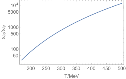
In the numerical studies below, we concentrate only on computation of the disparity (33) while the background approximation (20) remains valid. The generalization of this result on the case when the critical value $a_{c}$ becomes large is straightforward and discussed in Section IV.2.

Therefore, we model $a(t)$ to be increasing with time from zero and (smoothly) stops at some cutoff value $a_{c}\leq 1$ corresponding to the decoherence moment $t_{\rm dec}$, i.e.

$$a(s)=a_{c}\tanh\left(\frac{s}{s_{c}}\right),~{}~{}~{}~{}~{}~{}s\equiv t/R_{0}$$ (45)

where $a_{c}$ and $s_{c}$ serve as two free parameters. For convenience in numerical computation, we use the “rescaled” time $s\equiv t/R_{0}$ in this appendix. The parameter $a_{c}$ is defined by (31) and corresponds to the moment when the axion field loses its coherence as explained above and in footnote 5. The parameter $s_{c}$ describes the rate the parameter $a(t)$ changes with time.

As manifested in numerical evaluation, the final effects of the disparity (33) do not depend on what the exact model for $a(t)$ is. More specifically, the rate of the variation of $a(t)$ does not affect the final magnitude of the disparity between two species. Here we model it as the hyperbolic tangent form just for the convenience of numerical calculations. In the model (45), we describe the critical point using the cutoff $a_{c}$. As one can see from Fig. 3, the final disparity effects do not depend on parameter $s_{c}$, but only depend on the value of $a_{c}$ when the coherence of the axion field is lost. The Fig. 3 also shows that the disparity effects do not depend on the axion mass $m_{a}$, in agreement with our arguments in Section IV.1.

The disparity effects also do not depend on the viscosity $\eta$. To support this claim we did two different computations with different values of viscosity. The first choice is motivated by our previous studies [4] where we used $\eta\simeq m_{\pi}^{3}$ which has been computed in different models under different conditions in refs [63, 64]. It is known that the viscosity is in fact is somewhat larger in the region of sufficiently high temperature. Therefore, as the second choice we use the holographic arguments of ref. [65] suggesting that $\eta$ could be one order of magnitude larger than conventional perturbative QCD predicts (we use factor 8.4 in our numerical computations). One can explicitly see from Fig. 5 that the final destination for the disparity effects do not depend on the viscosity, in agreement with general arguments of Section IV.1.

We summarize the numerical values of other parameters and constants needed in calculations in Table. 1. We choose initial temperature $T_{0}$ as $200$ MeV. The (anti)nuggets evolves in the background axion field from $200$ MeV to the QCD transition temperature $170$ MeV, and we can safely take the temperature as a constant, $T/T_{0}\simeq 1$.

Table 1: Table for some numerical parameters

Quantity	Value	QCD units ($m_{\pi}=1$)
flavours $N_{f}$	2	2
colors $N_{c}$	3	3
degeneracy factor (in) $g^{\rm in}$	12	12
degeneracy factor (out) $g^{\rm out}$	37	37
bag constant $E_{B}$	$(150~{}\rm{MeV})^{4}$	$1.5$
“squeezer” parameter $\mu_{1}$	330 MeV	2.4
initial temperature $T_{0}$	200 MeV	1.5
QCD viscosity $\eta$  [63, 64]	0.002 GeV3	1
QCD viscosity $\eta$ [65]	0.02 GeV3	8.4
axion decay constant $f_{a}$	$10^{10}$ GeV	$7.4\times 10^{10}$
mass of axion $m_{a}$	$10^{-4}$eV	$7\times 10^{-13}$
mass of axion $m_{a}$	$10^{-6}$ eV	$7\times 10^{-15}$
domain wall tension $\sigma(m_{a}\sim 10^{-4}$eV)	$9\times 10^{5}$ GeV3	$3.7\times 10^{8}$
domain wall tension $\sigma(m_{a}\sim 10^{-6}$eV)	$9\times 10^{7}$ GeV3	$3.7\times 10^{10}$
initial radius $R_{0}\sim m_{a}^{-1}$	$0.2$ cm	$1.4\times 10^{12}$
initial radius $R_{0}\sim m_{a}^{-1}$	$20$ cm	$1.4\times 10^{14}$

(a) $s_{c}=10^{-2}$

(b) $s_{c}=10^{-5}$

Figure 3: Numerical solutions of (anti)nuggets evolving in the background of axion field before QCD transition. The blue and orange lines represent the evolutions of $R^{-}(s)$ and $R^{+}(s)$ respectively. We plot the upper four subfigures in (a) with $s_{c}=10^{-2}$ and the lower four subfigures in (b) with $s_{c}=10^{-5}$. The numerical values of parameters $m_{a}$ and $a_{c}$ that we use in calculating each subfigure can be seen in the upper edge and right edge of the graph.

Figure 4: The first few oscillations of $R^{+}$ in the lower left subfigure of Fig. 3. We choose this as an example to show that there is no cuspy problem.

Figure 5: Dependence on viscosity $\eta$. Amplitudes of $R^{-}$ (blue) and $R^{+}$ (orange) are plotted. The solid lines correspond to $\eta=8.4m_{\pi}^{3}(\times 10^{9})$, and the dashed lines correspond to $\eta=1.0m_{\pi}^{3}(\times 10^{9})$. Here parameters $m_{a}=10^{-4}$ eV and $s_{c}=10^{-5}$ are chosen.

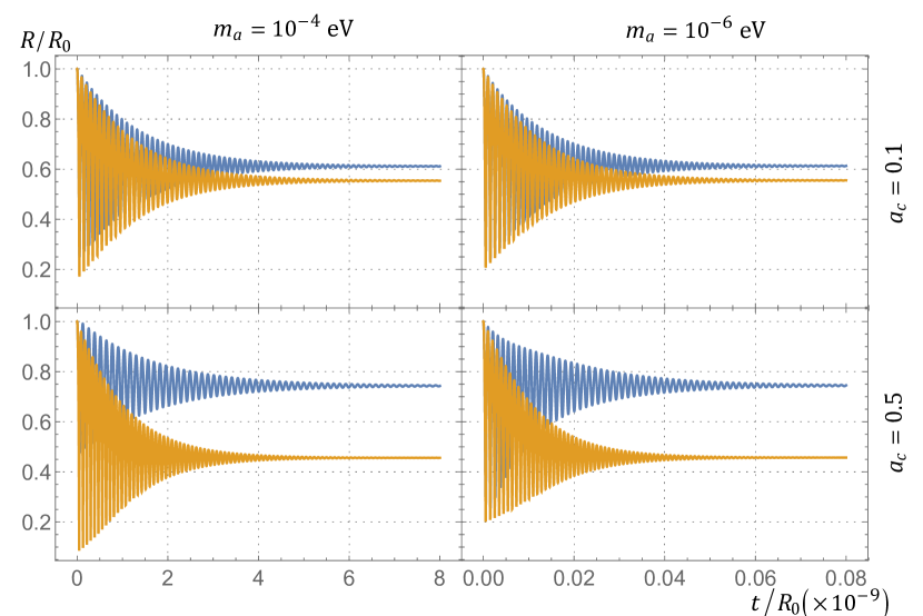
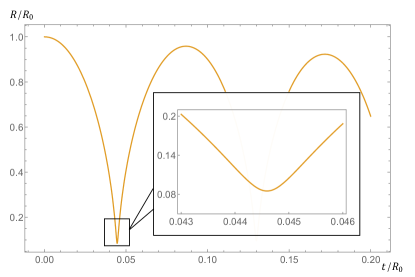
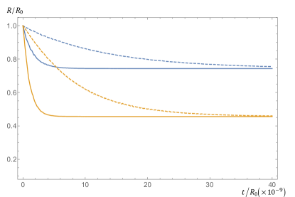
In Fig. 3(a), we draw $2\times 2$ subfigures , for $m_{a}\simeq(10^{-4},~{}10^{-6})$ eV, $a_{c}=(0.1,0.5)$ and we set the parameter $s_{c}=10^{-2}$. We set the viscosity as $\eta=8.4~{}m_{\pi}^{3}$. The Fig. 3(b) is the same as the Fig. 3(a) but with a different parameter $s_{c}=10^{-5}$. The blue and orange lines represent the evolution of $R^{-}(s)$ and $R^{+}(s)$ respectively. The difference between these two kinds of lines is the accumulated disparity effects. Comparing Fig. 3(a) with Fig. 3(b), we see that changing $s_{c}$ will not affect the disparity effects. This verifies that the difference between two kinds of nuggets is non-sensitive to how $a$ increases, fast or slow. In Fig. 3(a) or Fig. 3(b), comparing the four subfigures horizontally with $a_{c}$ fixed and $m_{a}$ varied, we see that the disparity effects are independent of $m_{a}$. This supports the arguments in Section IV.1 that the disparity effects are non-sensitive to the mass of axion. Then we compare the four subfigures vertically with $a_{c}$ varied and $m_{a}$ fixed. We see that the disparity effects are determined by $a_{c}$ rather than other parameters. For $a_{c}=0.1$, we see that $\Delta R_{\rm form}=\left|R^{+}_{\rm form}-R^{-}_{\rm form}\right|\simeq 0.06$ and $\left<R_{\rm form}\right>=\frac{1}{2}\left|R^{+}_{\rm form}+R^{-}_{\rm form}\right|\simeq 0.6$, consistent with the analytical relation (32) in Section III. For $a_{c}=0.5$, $\Delta R_{\rm form}\simeq 0.3$ and $\left<R_{\rm form}\right>\simeq 0.6$, again consistent with the relation (32).

We also notice that the oscillations shown on Fig. 3 are very sharp. But these seemingly cuspy behaviour is in fact quite smooth on the QCD scale. To see this, we zoom in the first few oscillations of $R^{+}$ in the lower left subfigure of Fig. 3(a), and plot it in Fig. 4. We see that the duration of “cusp” is $\delta t_{\rm cusp}\sim 10^{-3}R_{0}$, which is much longer than the QCD scale $\delta t_{\rm cusp}\gg\Lambda_{\rm QCD}^{-1}$. One should also add that the oscillation frequency is not sensitive to the viscosity $\eta$ according to eq. (27b). Therefore, our comment about “non-cuspy” behaviour remains unaffected as the time scale of a single oscillation (and therefore $\delta t_{\rm cusp}$) is not sensitive to the viscosity $\eta$.

Appendix E Fermi integrals

We now study some more details on the Fermi integral of the following form:

$$I_{n}(b)=\int_{0}^{\infty}\frac{dx\cdot x^{n-1}}{e^{x-b}+1}.$$ (46)

Such integrals can be exactly solved in terms of the so-called “polylog” function of degree $n$:

$${\rm Li}_{n}(z)=\sum_{k=1}^{\infty}\frac{1}{k^{n}}z^{k}.$$ (47)

Specifically, we obtain the following exact solution:

$$I_{n}(b)=-\Gamma(n){\rm Li}_{n}(-e^{b}).$$ (48)

where $\Gamma(n)$ is the gamma function. Also, one may find the polylog function satisfies following property when doing derivation:

$$\frac{d}{db}{\rm Li}_{n}(-e^{b})={\rm Li}_{n-1}(-e^{b}).$$ (49)

This property implies a useful relation between different $I_{n}$’s:

$$\frac{d}{db}I_{n}(b)=(n-1)I_{n-1}(b).$$ (50)

For $b\geq 0$, we sometimes prefer to approximate $I_{n}(b)$ in terms of “basic” functions:

$$I_{1}(b)=\ln(1+e^{b})\quad\qquad\qquad\qquad\qquad({\rm Exact})$$ (51a)

$$I_{2}(b)\simeq\frac{\pi^{2}}{6}+\frac{1}{2}b^{2}-\frac{\pi^{2}}{12}e^{-b}\qquad~{}\quad\qquad(\pm 2\%)$$ (51b)

$$I_{3}(b)\simeq\frac{\pi^{2}}{3}b+\frac{1}{3}b^{3}+\frac{3}{2}\zeta(3)\cdot e^{-b}\quad\qquad(\pm 2\%)$$ (51c)

$$I_{4}(b)\simeq\frac{7\pi^{4}}{60}+\frac{\pi^{2}}{2}b^{2}+\frac{1}{4}b^{4}-\frac{7\pi^{4}}{120}e^{-b}\quad(\pm 3\%)$$ (51d)

All approximations are highly accurate within $\pm 3\%$ uncertainty. Other useful approximations can be writing higher order $I_{n}(b)$ in terms of $I_{2}(b)$. For examples,

$$\frac{I_{3}(b)}{I_{2}(b)}\simeq\frac{3}{2}+\frac{2}{3}\sqrt{I_{2}(b)}\qquad\qquad(\underbrace{\pm 5\%}_{b\leq 5};~{}\underbrace{\pm 10\%}_{b\leq 10}).$$ (52)

Note that $\mu_{\rm max}\simeq 500$ MeV is the critical upper limit of QCD cutoff and $T\gtrsim 170$ MeV before QCD transition, thus $b\lesssim 3$ is the full applicable domain in this present work of study. A similar approximation for $I_{4}(b)$ is

$$I_{4}(b)\simeq 2\pi I_{2}(b)+(I_{2}(b))^{2}\qquad\qquad\qquad(\underbrace{\pm 3\%}_{b\leq 10}).$$ (53)

Also, before transition, $T\gtrsim 170$ MeV. Thus, this approximation is within $5\%$ of error since $b\lesssim 3$. Also, near the transition $T\lesssim 220$ MeV, we can also approximate

$$b^{2}\simeq 2.92+2I_{2}(b)\qquad\qquad\qquad\quad\qquad(\underbrace{\pm 3\%}_{b\geq 1.5}),$$ (54)

which is a valid approximation for $\mu>\mu_{1}\simeq 330$ MeV.

References

- [1] A. R. Zhitnitsky, JCAP 0310, 010 (2003) [hep-ph/0202161].
- [2] D. H. Oaknin and A. Zhitnitsky, Phys. Rev. D 71, 023519 (2005) [hep-ph/0309086].
- [3] E. Witten, Phys. Rev. D 30, 272 (1984).
- [4] X. Liang and A. Zhitnitsky, Phys. Rev. D 94, 083502 (2016) [arXiv:1606.00435 [hep-ph]].
- [5] Y. Aoki, G. Endrodi, Z. Fodor, S. D. Katz and K. K. Szabo, Nature 443, 675 (2006) [hep-lat/0611014].
-
[6]
R. D. Peccei and H. R. Quinn,
Phys. Rev. D 16, 1791 (1977);
S. Weinberg, Phys. Rev. Lett. 40, 223 (1978);
F. Wilczek, Phys. Rev. Lett. 40, 279 (1978). -
[7]
J.E. Kim, Phys. Rev. Lett. 43 (1979) 103;
M.A. Shifman, A.I. Vainshtein, and V.I. Zakharov, Nucl. Phys. B166 (1980) 493(KSVZ-axion). -
[8]
M. Dine, W. Fischler, and M. Srednicki, Phys. Lett. B104
(1981) 199;
A.R. Zhitnitsky, Yad.Fiz. 31 (1980) 497; Sov. J. Nucl. Phys. 31 (1980) 260 (DFSZ-axion). - [9] K. van Bibber and L. J. Rosenberg, Phys. Today 59N8, 30 (2006);
- [10] S. J. Asztalos, L. J. Rosenberg, K. van Bibber, P. Sikivie, K. Zioutas, Ann. Rev. Nucl. Part. Sci. 56, 293-326 (2006).
- [11] Pierre Sikivie, Lect. Notes Phys. 741, 19 (2008) arXiv:0610440v2 [astro-ph].
- [12] G. G. Raffelt, Lect. Notes Phys. 741, 51 (2008) [hep-ph/0611350].
- [13] P. Sikivie, Int. J. Mod. Phys. A 25, 554 (2010) [arXiv:0909.0949 [hep-ph]].
- [14] L. J. Rosenberg, Proc. Nat. Acad. Sci. (2015),
- [15] P. W. Graham, I. G. Irastorza, S. K. Lamoreaux, A. Lindner and K. A. van Bibber, Ann. Rev. Nucl. Part. Sci. 65, 485 (2015) [arXiv:1602.00039 [hep-ex]].
- [16] A. Ringwald, arXiv preprint (2016) [arXiv:1612.08933 [hep-ph]]
- [17] D. Budker, P. W. Graham, M. Ledbetter, S. Rajendran and A. Sushkov, Phys. Rev. X 4, no. 2, 021030 (2014) [arXiv:1306.6089 [hep-ph]].
- [18] P. W. Graham and S. Rajendran, Phys. Rev. D 88, 035023 (2013) [arXiv:1306.6088 [hep-ph]].
- [19] G. Rybka, A. Wagner, A. Brill, K. Ramos, R. Percival and K. Patel, Phys. Rev. D 91, no. 1, 011701 (2015) [arXiv:1403.3121 [physics.ins-det]].
- [20] P. Sikivie, N. Sullivan and D. B. Tanner, Phys. Rev. Lett. 112, no. 13, 131301 (2014) [arXiv:1310.8545 [hep-ph]].
- [21] C. Beck, Phys. Rev. Lett. 111, 231801 (2013), [arxiv:1309.3790[hep-ph]];
- [22] Y. V. Stadnik and V. V. Flambaum, Phys. Rev. D 89, no. 4, 043522 (2014) [arXiv:1312.6667 [hep-ph]].
- [23] P. Sikivie, Phys. Rev. Lett. 113, no. 20, 201301 (2014) [arXiv:1409.2806 [hep-ph]].
- [24] B. T. McAllister, S. R. Parker and M. E. Tobar, Phys. Rev. Lett. 116, no. 16, 161804 (2016) Erratum: [Phys. Rev. Lett. 117, no. 15, 159901 (2016)] [arXiv:1512.05547 [hep-ph]].
- [25] C. T. Hill, Phys. Rev. D 91, no. 11, 111702 (2015) [arXiv:1504.01295 [hep-ph]].
- [26] C. T. Hill, Phys. Rev. D 93, no. 2, 025007 (2016) [arXiv:1508.04083 [hep-ph]].
- [27] Y. Kahn, B. R. Safdi and J. Thaler, Phys. Rev. Lett. 117, no. 14, 141801 (2016) [arXiv:1602.01086 [hep-ph]].
- [28] R. Barbieri et al., arXiv:1606.02201 [hep-ph].
- [29] A. Arvanitaki and A. A. Geraci, Phys. Rev. Lett. 113, no. 16, 161801 (2014) [arXiv:1403.1290 [hep-ph]].
- [30] R. Kitano and N. Yamada, JHEP 1510, 136 (2015) [arXiv:1506.00370 [hep-ph]].
- [31] C. Bonati, M. D’Elia, M. Mariti, G. Martinelli, M. Mesiti, F. Negro, F. Sanfilippo and G. Villadoro, JHEP 1603, 155 (2016) [arXiv:1512.06746 [hep-lat]].
- [32] S. Borsanyi et al., Nature 539, no. 7627, 69 (2016) [arXiv:1606.07494 [hep-lat]].
- [33] P. Petreczky, H. P. Schadler and S. Sharma, Phys. Lett. B 762, 498 (2016) [arXiv:1606.03145 [hep-lat]].
- [34] A. Zhitnitsky, Phys. Rev. D 74, 043515 (2006) [astro-ph/0603064].
- [35] A. Zhitnitsky, EPJ Web Conf. 137, 09014 (2017) doi:10.1051/epjconf/201713709014 [arXiv:1611.05042 [hep-ph]].
[36]
P. Sikivie,
Phys. Rev. Lett. 48 (1982) 1156;
A. Vilenkin and A.E. Everett, Phys. Rev. Lett. 48 (1982) 1867. - [37] A. Vilenkin, E.P.S. Shellard, “Cosmic strings and other topological defects”, Cambridge University Press, 1994
- [38] S. Chang, C. Hagmann and P. Sikivie, Phys. Rev. D 59, 023505 (1999) [hep-ph/9807374].
- [39] M. M. Forbes and A. R. Zhitnitsky, JHEP 0110, 013 (2001) [arXiv:hep-ph/0008315].
- [40] G. Gabadadze and M.A. Shifman, Phys. Rev.D 62(2000)114003 [arXiv:hep-ph/0007345].
- [41] D. T. Son, M. A. Stephanov and A. R. Zhitnitsky, Phys. Rev. Lett. 86, 3955 (2001) [hep-ph/0012041].
[42]
T.W.B. Kibble, J. Phys. A9, 1387 (1976);
W. Zurek, Nature 317, 505 (1985) - [43] W. Zurek, Phys. Rep. 276, 177 (1996)
[44]
O. Wantz and E. P. S. Shellard,
Phys. Rev. D 82, 123508 (2010)
[arXiv:0910.1066 [astro-ph.CO]].
O. Wantz and E. P. S. Shellard, Nucl. Phys. B 829, 110 (2010) [arXiv:0908.0324 [hep-ph]]. - [45] T. Hiramatsu, M. Kawasaki, K. Saikawa and T. Sekiguchi, Phys. Rev. D 85, 105020 (2012) Erratum: [Phys. Rev. D 86, 089902 (2012)] [arXiv:1202.5851 [hep-ph]].
- [46] M. Kawasaki, K. Saikawa and T. Sekiguchi, Phys. Rev. D 91, no. 6, 065014 (2015) [arXiv:1412.0789 [hep-ph]].
- [47] L. Fleury and G. D. Moore, JCAP 1601, 004 (2016) [arXiv:1509.00026 [hep-ph]].
[48]
J. Preskill, M. B. Wise, and F. Wilczek, Phys.Lett. B120, 127 (1983);
L. Abbott and P. Sikivie, Phys.Lett. B 120, 133 (1983);
M. Dine and W. Fischler, Phys.Lett. B 120, 137 (1983). - [49] M. G. Alford, A. Schmitt, K. Rajagopal and T. Schäfer, Rev. Mod. Phys. 80, 1455 (2008) [arXiv:0709.4635 [hep-ph]]
- [50] K. Rajagopal and F. Wilczek, In *Shifman, M. (ed.): At the frontier of particle physics, vol. 3* 2061-2151 [hep-ph/0011333].
- [51] A. R. Zhitnitsky, Nucl. Phys. A 921, 1 (2014) [arXiv:1308.0020 [hep-ph]].
- [52] A. D. Sakharov, JETP Lett. 5, 24 (1967).
- [53] M. D’Elia and F. Negro, Phys. Rev. D 88, no. 3, 034503 (2013) [arXiv:1306.2919 [hep-lat]].
- [54] C. Bonati, M. D’Elia, H. Panagopoulos and E. Vicari, Phys. Rev. Lett. 110, no. 25, 252003 (2013) [arXiv:1301.7640 [hep-lat]].
- [55] C. Bonati, JHEP 1503, 006 (2015) [arXiv:1501.01172 [hep-lat]].
- [56] C. Bonati, M. D’Elia and A. Scapellato, Phys. Rev. D 93, no. 2, 025028 (2016) [arXiv:1512.01544 [hep-lat]].
- [57] K. Lawson and A. R. Zhitnitsky, Phys. Rev. D 95, no. 6, 063521 (2017) [arXiv:1510.07646 [astro-ph.HE]].
- [58] A. Zhitnitsky, arXiv:1707.03400 [astro-ph.SR].
- [59] C. Cao and A. Zhitnitsky, Phys. Rev. D 96, no. 1, 015013 (2017) [arXiv:1702.00012 [hep-ph]].
- [60] G. ’t Hooft, Phys. Rev. D 14, 3432 (1976).
- [61] T. Schafer and E. V. Shuryak, Rev. Mod. Phys. 70, 323 (1998).
- [62] R. Rapp, T. Sch fer, E. V. Shuryak and M. Velkovsky, Annals Phys. 280, 35 (2000) [hep-ph/9904353].
- [63] P. B. Arnold, G. D. Moore and L. G. Yaffe, JHEP 0011, 001 (2000) [hep-ph/0010177].
- [64] Jiunn-Wei Chen and Eiji Nakano. Phys. Lett. B 647, 371 (2007).
- [65] P. K. Kovtun, D. T. Son, and A. O. Starinets, Phys. Rev. Lett. 94, 111601 (2005) [arXiv:hep-th/0405231v2]