Newtonian self-gravity in trapped quantum systems and experimental tests

Abstract

No experimental evidence exists, to date, whether or not the gravitational field must be quantised. Theoretical arguments in favour of quantisation are inconclusive. The most straightforward alternative to quantum gravity, a coupling between classical gravity and quantum matter according to the semi-classical Einstein equations, yields a nonlinear modification of the Schrödinger equation. Here, effects of this so-called Schrödinger-Newton equation are discussed, which allow for technologically feasible experimental tests.

1 Introduction

The question how to reconcile the foundations of quantum theory with the dynamical space-time structure of general relativity is often reduced to problems arising at the Planck scale, e. g. in the physics of black holes or the early universe. Nonetheless, the status of the description of both gravity and quantum matter in a common framework is far from clear also at low energies: certainly from the point of view of experimental observations, but also from a theoretical perspective.

An illustrative example is the familiar double-slit experiment, if conducted with a massive particle. Assume a high sensitivity gravitational probe (a test mass attached to a sophisticated force metre) could be placed behind the slit, sensing the gravitational field of the spatial superposition state prepared by the slit. What is the gravitational field it would observe?

In analogy to electrodynamics one is tempted to think that the answer is obvious: The gravitational field should be in a superposition state itself, which is entangled with the particle state. However, the analogy between gravity and electrodynamics must eventually fail; at the latest when it comes to the question of renormalisability. One may, therefore, ask whether this analogy is still appropriate for the case of macroscopic non-classical states at low energy. In general relativity, on the other hand, the gravitational field is an expression of the space-time structure. Matter acts as a source, determining the curvature of space time. In the presence of quantised matter fields, one would ask: how does this quantum matter in a non-localised state source the gravitational field?

Keeping the classical space-time structure of general relativity, and treating quantum fields—which are then living on this curved space-time—as a curvature source, gives rise to the idea of (fundamentally) semi-classical gravity. The seemingly most straightforward way to incorporate quantum matter as a source into Einstein’s equations is to replace the classical stress-energy tensor by the expectation value of the corresponding quantum operator:

$$R_{\mu\nu}-\frac{1}{2}\,g_{\mu\nu}\,R=\frac{8\pi\,G}{c^{4}}\,\langle\Psi|\hat{T}_{\mu\nu}|\Psi\rangle$$ (1)

These are the semi-classical Einstein equations which have first been proposed in this context by Møller [1] and Rosenfeld [2].

Arguments have been invoked attempting to rule out this type of coupling between quantum matter and gravity solely on theoretical grounds. It has been pointed out that Eq. (1) is incompatible with both an instantaneous wave-function collapse and a no-collapse interpretation of quantum mechanics [3]. Nonetheless, this leaves open the possibility of a dynamical collapse in the spirit of collapse models [4]. More general assertions against any type of semi-classical coupling [5] were found inconclusive [6, 7, 8]. It seems that Rosenfeld was right when emphasising the necessity of experimental tests whether or not the gravitational field should be quantised: “There is no denying that, considering the universality of the quantum of action, it is very tempting to regard any classical theory as a limiting case to some quantal theory. In the absence of empirical evidence, however, this temptation should be resisted. The case for quantizing gravitation, in particular, far from being straightforward, appears very dubious on closer examination.” [2]

It was Carlip [9] who first pointed out that an experimental test of semi-classical gravity could be feasible in the nonrelativistic, low-energy limit of laboratory quantum systems. While the proposed test in matter wave interferometry experiments turned out to still be five to six orders of magnitude beyond the state of the art [10], tests in optomechanical set-ups are at the edge of feasible observations [11, 12].

Here, the underlying physics behind these proposed tests is reviewed. In section 2 the nonrelativistic limit of Eq. (1) to the so-called Schrödinger-Newton (SN) equation is discussed, followed by a review of how one obtains an equation for the centre of mass of a many-particle system in section 3. Effects of this modification of the Schrödinger equation in a harmonic oscillator are analysed in section 4 with a discussion of the possibilities for testing them in section 5. Some open questions are addressed in the conclusion section 6.

2 Semi-classical gravity in the nonrelativistic limit

Starting with the classical Einstein equations for a classical Klein-Gordon (or Dirac) field, one can show that the gravitational self-coupling is promoted to the Schrödinger equation (as a differential equation for the evolution of a classical field) obtained in the nonrelativistic ($c\to\infty$) limit [13], where it yields the nonlinear one-particle SN equation:

$$\mathrm{i}\hbar\frac{\partial}{\partial t}\psi(t,\mathbf{r})=\left(-\frac{\hbar^{2}}{2m}\nabla^{2}-Gm^{2}\int\mathrm{d}^{3}\mathbf{r}^{\prime}\,\frac{\left|\psi(t,\mathbf{r}^{\prime})\right|^{2}}{\left|\mathbf{r}-\mathbf{r}^{\prime}\right|}\right)\psi(t,\mathbf{r})\,.$$ (2)

For a quantum field, coupling to gravity according to Eq. (1), one can proceed in a similar fashion [14]. In the nonrelativistic, weak coupling limit, Einstein’s equations yield the Poisson equation $\nabla^{2}V=4\pi G\,m\,\langle\Psi\mid\hat{\psi}^{\dagger}\hat{\psi}\mid\Psi\rangle$, while the field equations on curved space-time limit to the Fock space Schrödinger equation including the solution $V$ of this Poisson equation as a nonlinear potential. The sectors belonging to different particle numbers separate in the nonrelativistic limit. In conclusion, one ends up with the $N$-particle equation [15]

$$\mathrm{i}\hbar\frac{\partial}{\partial t}\Psi(t,\mathbf{r}_{1},\cdots,\mathbf{r}_{N}) =\biggl{(}-\sum_{i=1}^{N}\frac{\hbar^{2}}{2m_{i}}\nabla^{2}_{i}+V_{\text{ext}}+V_{g}[\Psi]\biggr{)}\Psi(t;\mathbf{r}_{1},\cdots\mathbf{r}_{N})$$ (3a)

$$V_{g}[\Psi](t,\mathbf{r}_{1},\cdots,\mathbf{r}_{N}) =-G\sum_{i=1}^{N}\sum_{j=1}^{N}m_{i}m_{j}\int\mathrm{d}^{3}\mathbf{r}_{1}^{\prime}\cdots\mathrm{d}^{3}\mathbf{r}_{N}^{\prime}\frac{\left|\Psi(t;\mathbf{r}^{\prime}_{1},\cdots,\mathbf{r}^{\prime}_{N})\right|^{2}}{\left|\mathbf{r}_{i}-\mathbf{r}^{\prime}_{j}\right|}\,,$$ (3b)

where $V_{\text{ext}}$ stands for any additional non-gravitational potentials. Eq. (3) contains both the mutual gravitational interactions between particles and the gravitational self-interaction of each particle. In the one-particle case, $N=1$, one obtains Eq. (2).

3 The Schrödinger-Newton equation for the centre-of-mass motion

Contrary to linear interaction potentials, the wave-function dependent potential (3b) does not separate into centre of mass and relative coordinates exactly. Note, however, that the electromagnetic forces which determine the shape of a complex quantum system like a large molecule are considerably stronger than the gravitational forces. One can, therefore, make use of an approximation similar to the Born–Oppenheimer approximation in atom physics [16]. The characteristic time scale of the relative motion, dominated by the electromagnetic interactions, is much shorter than that of the centre of mass motion, which is only affected by self-gravitational forces. The potential (3b) can then be averaged over the relative degrees of freedom, resulting in a potential that only depends on the centre of mass coordinate, and in the following centre of mass SN equation:

$$\mathrm{i}\hbar\frac{\partial}{\partial t}\psi(t,\mathbf{r}) =\left(-\frac{\hbar^{2}}{2\,M}\nabla^{2}+V_{\text{ext}}+V_{g}[\psi]\right)\,\psi(t,\mathbf{r})$$ (4a)

$$V_{g}[\psi](t,\mathbf{r}) =-G\,\int\mathrm{d}^{3}\mathbf{r}^{\prime}\,\left|\psi(t,\mathbf{r^{\prime}})\right|^{2}\,I_{\rho_{c}}(\mathbf{r}-\mathbf{r^{\prime}})$$ (4b)

$$I_{\rho_{c}}(\mathbf{d}) =\int\mathrm{d}^{3}\mathbf{u}\,\mathrm{d}^{3}\mathbf{v}\,\frac{\rho_{c}(\mathbf{u})\,\rho_{c}(\mathbf{v}-\mathbf{d})}{\left|\mathbf{u}-\mathbf{v}\right|}\,,$$ (4c)

where $$M \psi \rho_{c} \chi$$ is the total mass, the centre of mass wave-function, and is the (averaged) mass distribution of the quantum system, defined from the relative wave-function as

$$\rho_{c}(\mathbf{r})=\sum_{i=1}^{N-1}m_{i}\int\mathrm{d}^{3}\mathbf{r}_{1}\cdots\mathrm{d}^{3}\mathbf{r}_{i-1}\,\mathrm{d}^{3}\mathbf{r}_{i+1}\cdots\mathrm{d}^{3}\mathbf{r}_{N-1}\left|\chi(\mathbf{r}_{1},\dots,\mathbf{r}_{i-1},\mathbf{r},\mathbf{r}_{i+1},\dots,\mathbf{r}_{N-1})\right|^{2}\,.$$ (4d)

Now, if the size of the considered system (e. g. molecule) is small compared to the extent of its centre of mass wave-function, $\rho_{c}$ can be approximated by a delta distribution, and Eq. (4) is approximately equivalent to the one-particle equation (2).

If the width of the wave-function becomes comparable to the size of the system then its structure, represented by the function $I_{\rho_{c}}$, must be taken into account. For a homogeneous spherical particle of radius $R$, for instance, one finds

$$I_{\rho_{c}}^{\text{sphere}}(d)=\frac{M^{2}}{R}\times\begin{cases}\frac{6}{5}-2\left(\frac{d}{2R}\right)^{2}+\frac{3}{2}\left(\frac{d}{2R}\right)^{3}-\frac{1}{5}\left(\frac{d}{2R}\right)^{5}&\text{for}\ d\leq 2R\,,\\ \frac{R}{d}&\text{for}\ d\geq 2R\,.\end{cases}$$ (5)

A more realistic model of a molecule also takes into account the crystalline structure of the atoms. A spherical particle of radius $R$ with atoms localised with a Gaussian distribution of width $\sigma$ is well approximated by the function [12, 17]

$$I_{\rho_{c}}^{\text{cryst}}(d)\approx\frac{6\,M^{2}}{5\,R}+\frac{M\,m_{\text{atom}}}{d}\,\mathrm{erf}\left(\frac{d}{\sqrt{2}\,\sigma}\right)\,,$$ (6)

as long as the wave-function has an extent small compared to the radius $R$ of the whole particle. The first term stems from the mutual gravitational attraction of the atoms, while the second term describes the accumulated self-gravitation forces of each atom with its own marginal wave-function.

In the narrow wave-function regime, where the extent of the wave-function is small also compared to the localisation length $\sigma$ of the atoms, the error function can be expanded around $d=0$, yielding the quadratic approximation

$$I_{\rho_{c}}^{\text{narrow}}(d)\approx\frac{6\,M^{2}}{5\,R}+\frac{2\,M\,m_{\text{atom}}}{\sqrt{2\pi}\sigma}\,\left(1-\frac{d^{2}}{6\,\sigma^{2}}\right)\,.$$ (7)

4 Effects on harmonically trapped quantum systems

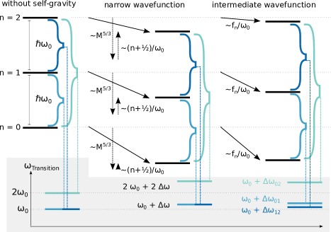
Figure 1: Schematic picture of the self-gravitational effect on the harmonic oscillator spectrum in the narrow and intermediate wave-function regime [12].

We assume that the potential $V_{\text{ext}}$ is such that it strongly confines the wave-function in the $y$- and $z$-direction. Then the SN equation can be shown to become effectively one-dimensional [17]. If we assume a quadratic potential in the $x$-direction, $V_{\text{ext}}=M\,\omega_{0}^{2}\,x^{2}/2$, then for the narrow wave-function regime, using Eq. (7), one obtains the Hamiltonian

$$H^{\text{narrow}} =-\frac{\hbar^{2}}{2\,M}\nabla^{2}+\frac{M}{2}\omega_{0}^{2}\,x^{2}-\frac{6\,G\,M^{2}}{5\,R}-\frac{2\,G\,M\,m_{\text{atom}}}{\sqrt{2\pi}\sigma}\,\left(1-\frac{x^{2}-2\,x\,\langle x\rangle+\langle x^{2}\rangle}{6\,\sigma^{2}}\right)$$

$$=-\frac{\hbar^{2}}{2\,M}\nabla^{2}+\frac{M}{2}\omega_{\text{SN}}^{2}\,\langle x^{2}\rangle-M\,\omega_{\text{SN}}^{2}\,x\,\langle x\rangle+\frac{M}{2}\left(\omega_{0}^{2}+\omega_{\text{SN}}^{2}\right)x^{2}+\text{const.}\,,$$ (8)

with

$$\omega_{\text{SN}} =\sqrt{\sqrt{\frac{2}{\pi}}\frac{G\,m_{\text{atom}}}{3\,\sigma^{3}}}\,.$$ (9)

For a wave-function comparable to the atom localisation scale, the Hamiltonian becomes a much more complicated nonlinear functional. However, for the sake of determining the distortion of the energy spectrum one can simply use first order perturbation theory. The potential (4b) evaluated for the unperturbed eigenstates $\psi_{n}^{(0)}$ is then treated as a perturbation, yielding the energy shift

$$\Delta E_{n}=\langle\psi^{(0)}_{n}\mid V_{g}[\psi^{(0)}_{n}](\mathbf{r})\mid\psi^{(0)}_{n}\rangle=-\frac{G\,\hbar\,m_{\text{atom}}}{4\,\sigma^{3}\,\omega_{0}}\,f_{n}(\alpha)\,,\quad\quad\text{with}\quad\quad\alpha=2\sigma\,\sqrt{\frac{M\omega_{0}}{\hbar}}\,.$$ (10)

In the case of the narrow wave-function, the function $f_{n}$ depends on the quantum number $n$ linearly, implying that the energy gap between eigenstates changes to $\Delta n\,\hbar\omega_{0}\,(1+\omega_{\text{SN}}^{2}/\omega_{0}^{2})$. Nonetheless, the transition energy only depends on the difference $\Delta n=(n_{1}-n_{2})$, not on $n_{1}$ and $n_{2}$ explicitly.

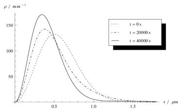
Figure 2: Inhibitions of the free dispersion of a wave packet. Plotted is the radial probability density $\rho=4\pi\,r^{2}\,\left|\psi\right|^{2}$ for a mass of $7\times 10^{9}~{}\atomicmass$ (left) and $10^{10}~{}\atomicmass$ (right) at different times.

This changes in the regime of wider wave-functions, where $f_{n}$ becomes nonlinear in $n$ [12, 17]:

$$f_{n}(\alpha) \approx\text{const.}+\alpha^{3}\,\sqrt{\frac{2}{\pi}}\,\int_{0}^{\infty}\mathrm{d}\zeta\,\exp\left(-\frac{\alpha^{2}\,\zeta^{2}}{2}\right)\,P_{n}(\alpha\,\zeta)\,\left(\frac{\mathrm{erf}\left(\sqrt{2}\,\zeta\right)}{2\,\zeta}-\sqrt{\frac{2}{\pi}}\right)\,,$$ (11a)

$$P_{n}(z) =\frac{\mathrm{e}^{-z^{2}/2}}{\sqrt{2\pi}\,(2^{n}\,n!)^{2}}\,\int_{-\infty}^{\infty}\mathrm{d}\xi\,\mathrm{e}^{-2\xi^{2}}\,H_{n}\left(\xi\right)^{2}\left(\mathrm{e}^{2\,z\,\xi}\,H_{n}\left(\xi-z\right)^{2}+\mathrm{e}^{-2\,z\,\xi}\,H_{n}\left(\xi+z\right)^{2}\right)\,,$$ (11b)

where $H_{n}$ are the Hermite polynomials. Now the frequency gap between adjacent energy levels depends on $n_{1}$, $n_{2}$ explicitly, yielding a fine structure for the transition frequencies as depicted in Fig. 1.

Instead of the energy spectrum, one can study the effect of the self-gravitational potential on the dynamics of a quantum harmonic oscillator. For a squeezed coherent (i. e. Gaussian) state, the dynamics can be reduced to a set of two differential equations for the first and second moments:

$$0 =\frac{\mathrm{d}^{2}}{\mathrm{d}t^{2}}\langle x\rangle+\omega_{0}^{2}\langle x\rangle$$ (12a)

$$0 =\frac{\mathrm{d}^{3}}{\mathrm{d}t^{3}}\langle(x-\langle x\rangle)^{2}\rangle+4\,\left(\omega_{0}^{2}+\omega_{\text{SN}}^{2}[\psi]\right)\,\frac{\mathrm{d}}{\mathrm{d}t}\langle(x-\langle x\rangle)^{2}\rangle\,.$$ (12b)

The first equation describes the usual oscillation of the centre of the wave-function with the unperturbed trap frequency $\omega_{0}$. The second equation describes the internal oscillation, for which the frequency is shifted by a factor of $\sqrt{1+\omega_{\text{SN}}^{2}/\omega_{0}^{2}}$.

In the general case of a wider wave-function this frequency shift depends on the wave-function. However, it is strongest for a narrow wave-function, where $\omega_{\text{SN}}$ takes the value (9). For a wider wave-function, the self-gravitational effect only becomes less significant. The effect in the narrow regime was discussed by Yang et al. [11].

5 Experimental tests

First ideas to test the SN equation experimentally [9] were based on the loss of interference in matter-wave interferometry experiments [18]. Current experiments reach masses of up to $10^{4}~{}\atomicmass$ and are clearly in the wide wave-function regime were Eq. (2) is valid. Numerical and analytical estimates [10] yield a required mass around $10^{10}~{}\atomicmass$ for a micrometre sized wave packet to show significant inhibitions of the free dispersion, see Fig. 2 for example plots of the evolution of a Gaussian wave packet. The required mass values seem infeasible on Earth, although they might be achievable in space experiments [19]. Note also that for the required mass scales, the effects of the internal structure of the particles are no longer negligible and, therefore, Eq. (2) is only of limited use for good predictions. However, approximation schemes exist [20, 21] which allow for a simple numerical calculation of the magnitude of the deviation between the nonlinear dynamics according to the SN equation and the ordinary, linear Schrödinger equation.

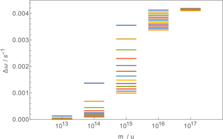
Figure 3: Resulting frequency spectrum of the transition frequency $\Delta\omega$ between adjacent eigenstates ($\Delta n=1$) for osmium at $T=100\,\mathrm{m}\mathrm{K}$, $\omega_{0}=2\pi\times 10\,\mathrm{s}^{-1}$.

As far as ground based experiments are concerned, the two effects discussed here for particles trapped in quadratic potentials seem the most promising routes towards an experimental test. A proposal for a test of the spectral effect was presented in Ref. [12]. It consists of a levitated osmium disc in a Paul trap which is cooled to a temperature below 100  m K . At this temperature osmium becomes superconducting, avoiding decoherence due to blackbody radiation. The suggested experimental parameters are a particle mass of $10^{14}~{}\atomicmass$ trapped at a frequency of 10  Hz . At these values, a frequency resolution of 0.1  m Hz  would be sufficient for a detection of the spectral fine structure due to the SN equation. Fig. 3 shows a quantitative plot of the expected frequency spectrum for these values. At low masses, self-gravity becomes negligible. At high masses all spectral lines are shifted equally. The intermediate regime, where a significant splitting appears, spans about 3 orders of magnitude in mass.

The crucial parameter for the choice of material is the Debye–Waller factor, which determines the localisation $\sigma$ of the atoms within the crystal. It takes an ideal value for osmium, even compared to materials of larger atomic mass such as gold; see Tab. 1 for a comparison of some materials. Levitation of a micrometre particle in a Paul trap has already been demonstrated experimentally [22], as have the low frequencies required [23], and the control of decoherence [24]. Cooling to low energy states has not been demonstrated for the required masses, but the technological tools exist.

The dynamical effects [11] are somewhat disadvantageous to observe: they require both preparation of a squeezed state and a larger mass in order to reach the narrow wave-function regime. On the other hand, the required set-up is closer to existing ones, such as cooled mirrors (e. g. LIGO or LISA pathfinder). The fact that all of these systems are based on silicon rather than osmium, however, requires another two orders of magnitude better resolution compared to the same system based on osmium (cf. Tab. 1). At 10  Hz  trap frequency, a quality factor better than $10^{6}$ is required [11]. The feasibility for a test in several systems has been examined in Ref. [25].

Table 1: Relevant experimental parameters for different materials [12].

Material	$m_{\text{atom}}$ / u	$\rho$ / g cm-3	$\sigma$ / pm	$\omega_{\text{SN}}^{2}/\omega_{0}^{2}$
Silicon	28.086	2.329	6.96	0.00246
Tungsten	183.84	19.30	3.48	0.128
Osmium	190.23	22.57	2.77	0.264
Gold	196.97	19.32	4.66	0.0574

6 Conclusion and open questions

From the above discussion we conclude that, although a realisation is still challenging, the SN equation seems testable with existing technology in the nearer future. What would we learn from such a test?

Obviously, if the predicted deviations from linear quantum mechanics would be observed, this would result in a complete paradigm shift of our view on both gravity and the foundations of quantum mechanics. If, on the other hand, standard quantum mechanics is confirmed and the SN equation ruled out by experiments (likely the outcome expected by a large majority of physicists) this would rule out the semi-classical Einstein equations (1) as a fundamental model. It would, however, not be conclusive evidence for the quantisation of gravity, since other types of coupling of quantum matter to a classical space-time could be possible, which do not yield the SN equation as a nonrelativistic limit. In fact, with stochastic gravity [26, 27] there is an example for such a model.

As the SN equation was first discussed by Diósi [15] and Penrose [28], it is often considered in context of the gravitational collapse model named after these two [29, 30, 31, 28, 32]. Although not directly related to it, one can discuss whether the SN equation could play a role in the collapse of the wave-function. On the one hand, the classicality of the gravitational force provides exactly the non-unitary ingredient needed for an objective collapse. On the other hand, the SN alone does not explain the emergence of classicality, since the SN “collapse” is completely deterministic. It does not recover the Born probability rule [14].

Probably the biggest concern against a fundamental validity of the SN equation is that measurements in the usual instantaneous collapse prescription allow for faster-than-light signalling when combined with a nonlinear dynamics [14]. It might be that a consistent description which makes use of semi-classical gravity as an explanation of the wave-function collapse can circumvent this problem. This description, however, has yet to be found.

The advances reviewed here resulted from collaborations with M. Bahrami, A. Bassi, J. Bateman, S. Donadi, D. Giulini, and H. Ulbricht. I gratefully acknowledge funding from the German Research Foundation (DFG) and the Italian National Institute for Nuclear Physics (INFN).

References

References

- [1] Møller C 1962 Colloques Internationaux CNRS vol 91 ed Lichnerowicz A and Tonnelat M A (CNRS, Paris)
- [2] Rosenfeld L 1963 Nucl. Phys. 40 353–356
- [3] Page D N and Geilker C D 1981 Phys. Rev. Lett. 47 979–982
- [4] Bassi A, Lochan K, Satin S, Singh T P and Ulbricht H 2013 Rev. Mod. Phys. 85 471–527 (Preprint 1204.4325)
- [5] Eppley K and Hannah E 1977 Found. Phys. 7 51–68
- [6] Mattingly J 2005 Einstein Studies Volume 11. The Universe of General Relativity Einstein Studies ed Kox A J and Eisenstaedt J (Boston: Birkhäuser) chap 17, pp 327–338
- [7] Kiefer C 2007 Quantum Gravity 2nd ed (International Series of Monographs on Physics vol 124) (Oxford: Clarendon Press)
- [8] Albers M, Kiefer C and Reginatto M 2008 Phys. Rev. D 78 064051 (Preprint 0802.1978)
- [9] Carlip S 2008 Class. Quantum Grav. 25 154010 (Preprint 0803.3456)
- [10] Giulini D and Großardt A 2011 Class. Quantum Grav. 28 195026 (Preprint 1105.1921)
- [11] Yang H, Miao H, Lee D S, Helou B and Chen Y 2013 Phys. Rev. Lett. 110 170401 (Preprint 1210.0457)
- [12] Großardt A, Bateman J, Ulbricht H and Bassi A 2016 Phys. Rev. D 93 096003 (Preprint 1510.01696)
- [13] Giulini D and Großardt A 2012 Class. Quantum Grav. 29 215010 (Preprint 1206.4250)
- [14] Bahrami M, Großardt A, Donadi S and Bassi A 2014 New J. Phys. 16 115007 (Preprint 1407.4370)
- [15] Diósi L 1984 Phys. Lett. A 105 199–202
- [16] Giulini D and Großardt A 2014 New J. Phys. 16 075005 (Preprint 1404.0624)
- [17] Großardt A, Bateman J, Ulbricht H and Bassi A 2016 Sci. Rep. 6 30840 (Preprint 1510.01262)
- [18] Arndt M and Hornberger K 2014 Nat. Phys. 10 271–277
- [19] Kaltenbaek R, Arndt M, Aspelmeyer M, Barker P F, Bassi A, Bateman J, Bongs K, Bose S, Braxmaier C, Brukner C, Christophe B, Chwalla M, Cohadon P F, Cruise A M, Curceanu C, Dholakia K, Döringshoff K, Ertmer W, Gieseler J, Gürlebeck N, Hechenblaikner G, Heidmann A, Herrmann S, Hossenfelder S, Johann U, Kiesel N, Kim M, Lämmerzahl C, Lambrecht A, Mazilu M, Milburn G J, Müller H, Novotny L, Paternostro M, Peters A, Pikovski I, Pilan-Zanoni A, Rasel E M, Reynaud S, Riedel C J, Rodrigues M, Rondin L, Roura A, Schleich W P, Schmiedmayer J, Schuldt T, Schwab K C, Tajmar M, Tino G M, Ulbricht H, Ursin R and Vedral V 2016 EPJ Quant. Tech. 3 5 (Preprint 1503.02640)
- [20] Großardt A 2016 Phys. Rev. A 94 022101 (Preprint 1503.02622)
- [21] Colin S, Durt T and Willox R 2016 Phys. Rev. A 93 062102 (Preprint 1402.5653)
- [22] Wuerker R F, Shelton H and Langmuir R V 1959 J. Appl. Phys. 30 342–349
- [23] Gerlich D 2003 Hyperfine Interactions 146-147 293–306 ISSN 0304-3843
- [24] Poulsen G, Miroshnychenko Y and Drewsen M 2012 Phys. Rev. A 86(5) 051402
- [25] Gan C, Savage C and Scully S 2016 Phys. Rev. D 93 124049
- [26] Hu B L and Verdaguer E 2008 Living Rev. Relativity 11 3
- [27] Anastopoulos C and Hu B L 2014 New J. Phys. 16 085007 arXiv:1403.4921 (Preprint 1403.4921)
- [28] Penrose R 1998 Phil. Trans. R. Soc. A 356 1927–1939
- [29] Diósi L and Lukács B 1987 Ann. Phys. (Berlin) 499 488–492
- [30] Diósi L 1989 Phys. Rev. A 40 1165–1174
- [31] Penrose R 1996 Gen. Relativ. Gravit. 28 581–600
- [32] Penrose R 2014 Found. Phys. 44 557–575