A Non-monotone Linear Search Method with Mixed Direction on Stiefel Manifold

Abstract

In this paper, we propose a non-monotone line search method for solving optimization problems on Stiefel manifold. Our method uses as a search direction a mixed gradient based on a descent direction, and a Barzilai-Borwein line search. Feasibility is guaranteed by projecting each iterate on the Stiefel manifold, through SVD factorizations. Some theoretical results for analyzing the algorithm are presented. Finally, we provide numerical experiments comparing our algorithm with other state-of-the-art procedures.

1 Introduction

In this paper we consider optimization in matrices with orthogonality constraints,

$$\min_{X\in\mathbb{R}^{n\times p}}\mathcal{F}(X)\quad s.t.\quad X^{\top}X=I$$ (1)

where $\mathcal{F}:\mathbb{R}^{n\times p}\rightarrow\mathbb{R}$ is a differentiable function and $I\in\mathbb{R}^{p\times p}$ is the identity matrix. The feasible set $St(n,p):=\{X\in\mathbb{R}^{n\times p}/X^{\top}X=I\}$ is known in the literature as the “Stiefel Manifold” which is reduced to the unit sphere when $p=1$ and in the case $p=n$ it is known as “Orthogonal group” (see Absil ). It is known that the dimension of the Stiefel manifold is $np-\frac{1}{2}p(p+1)$ Absil , and it can be seen as an embedded sub-manifold of $\mathbb{R}^{n\times p}$. Problem (1) encompasses many applications such as nearest low-rank correlation matrix problem Grubi ; Pietersz ; Rebonato , linear eigenvalue problem Golub ; Saad , Kohn-Sham total energy minimization YangMeza , orthogonal procrustes problem Elden ; Schonemann , weighted orthogonal procrustes problem Francis , sparse principal component analysis Ghaoui ; Journee ; Zou , joint diagonalization (blind source separation) Joho ; Theis , among others. In addition, many problems such as PCA, LDA, multidimensional scaling, orthogonal neighborhood preserving projection can be formulated as problem (1) Kokiopoulou . On the other hand, it is known that Stiefel manifold is a compact set which guarantees a global optimum, nevertheless it’s not a convex set which makes problem-solving (1) very hard. In particular, the quadratic assignment problem (QAP), which can be formulated as minimization over a permutation matrix in $\mathbb{R}^{n\times n}$, that is, $X^{\top}X=I$, $X\geq 0$ and “leakage interference minimization” LiuDai are NP-hard.

The problem (1) can be treated as a regular (vector) optimization problem, which conduces to several difficulties because orthogonal constraints can lead to many local minimizers. On the other hand, generating sequences of feasible points is not easy because preserving orthogonality constraints is numerically expensive. Most existing algorithms that generate feasible points either use routines to matrix reorthogonalization or generate points along geodesics on the manifold. The first one requires singular value decomposition or QR-decomposition, and the second one computes the matrix exponential or solves partial differential equations. We shall use the first approach. Some effort to avoid these approaches have been done, calculating inverse matrices instead of SVD’s at each step LaiOsher ; WenYang ; WenYin .

By exploiting properties of the Stiefel Manifold, we propose a non-monotone line search constraint preserving algorithm to solve problem (1) with a mixed gradient based search direction. We analyze the resulting algorithm, and compare it to other state-of-the-art procedures, obtaining promising numerical results.

1.1 Notation

We say that a matrix $W\in\mathbb{R}^{n\times n}$ is skew-symmetric if $W=-W^{\top}$. The trace of $X$ is defined as the sum of the diagonal elements which we will denote by $Tr[X]$. The Euclidean inner product of two matrices $A,B\in\mathbb{R}^{m\times n}$ is defined as $\langle A,B\rangle:=\sum_{i,j}a_{i,j}b_{i,j}=Tr[A^{\top}B]$. The Frobenius norm is defined by the above inner product, that is $||A||_{F}=\sqrt{\langle A,A\rangle}$. Let $\mathcal{F}:\mathbb{R}^{n\times p}\rightarrow\mathbb{R}$ be a differentiable function, we denote by $G:=\mathcal{DF}(X):=(\frac{\partial\mathcal{F}(X)}{\partial X_{ij}})$ the matrix of partial derivatives of $\mathcal{F}$. When evaluated at the current iterate $X_{k}$ of the algorithm, we denote the gradient by $G_{k}=\mathcal{DF}(X_{k})$. Other objects depending on $X_{k}$ are also denoted with subindex $k$. Additionally, the directional derivative of $\mathcal{F}$ along a given matrix $Z$ at a given point $X$ is defined by:

$$\mathcal{DF}(X)[Z]:=\lim_{t\rightarrow 0}\frac{\mathcal{F}(X+tZ)-\mathcal{F}(X)}{t}=\langle\mathcal{DF}(X),Z\rangle.$$ (2)

1.2 Organization

The rest of the paper is organized as follows. In section 2 we propose and analyze our mixed constraint preserving updating scheme. Subsubsection 2.1 establishes the optimality conditions, while subsection 2.2 is devoted to the projection operator on the Stiefel Manifold. The proposed updating scheme is introduced and analyzed in subsection 2.3. Two algorithms are presented in section 3. The first one uses Armijo line search, and the second one Barzilai-Borwein stepsize scheme. Finally, numerical experiments are carried out for comparing our algorithm with other state-of-the-art procedures by solving instances of Weighted Orthogonal Procrustes Problem (WOPP), Total Energy minimization, and Linear Eigenvalue problems, are presented in section 4.

2 A mixed constraint preserving updating scheme

2.1 Optimality conditions

The classical constrained optimization theory for continuous functions in $\mathbb{R}^{n}$ involve finding minimizers of the Lagrangean function applied to problem (1), given by:

$$\mathcal{L}(X,\Lambda)=\mathcal{F}(X)-\frac{1}{2}Tr[\,\Lambda^{\top}(X^{\top}X-I)\,],$$

where $\Lambda$ is the Lagrange multipliers matrix, which is a symmetric matrix because the matrix $X^{\top}X$ is also symmetric. The Lagrangean function leads to the first order optimality conditions for problem (1):

$$G-X\Lambda=0,$$ (3)

$$X^{\top}X-I=0.$$ (4)

By differentiating both sides of (4), we obtain the tangent space of Stiefel manifold at $X$:

$$T_{X}St(n,p):=\{Z\in\mathbb{R}^{n\times p}:X^{\top}Z+Z^{\top}X=0\}.$$

The following technical result, demonstrated by Wen-Yin in WenYin , provides a tool to calculate roots for Eqs. (3)-(4).

Lemma 1

Suppose that $X$ is a local minimizer of problem (1). Then $X$ satisfies the first order optimality conditions with the associated Lagrangian multiplier $\Lambda=G^{\top}X$. Define

$$\nabla\mathcal{F}_{1}(X):=G-XG^{\top}X\quad and\quad A:=GX^{\top}-XG^{\top}$$

then $\nabla\mathcal{F}_{1}(X)=AX$. Moreover, $\nabla\mathcal{F}_{1}=0$ if and only if $A=0$.

The lemma 1 establishes an equivalence to the Eq. (3) condition, i.e. $X\in\mathbb{R}^{n\times p}$ satisfies $\nabla\mathcal{F}_{1}(X)=0$ if and only if $X$ satisfies equation (3), so we can use this result as a stopping criterion for our algorithm.

2.2 Tools on Stiefel Manifold

The following lemma establishes an important property for matrices on Stiefel Manifold.

Lemma 2

If $X\in St(n,p)$ then $||X^{\top}M||_{F}^{2}\leq||M||_{F}^{2}$ for all $M\in\mathbb{R}^{n\times p}$ matrix.

Proof

In fact, let $X\in St(n,p)$ and $M\in\mathbb{R}^{n\times p}$, and let $X^{\top}=U_{X}\Sigma_{X}V_{X}^{\top}$, $M=U_{M}\Sigma_{M}V_{M}^{\top}$ be the singular value decomposition of $X^{\top}$ and $M$ respectively, where $\Sigma_{X}=diag(\sigma_{1},\sigma_{2},\ldots,\sigma_{p})\in\mathbb{R}^{p\times n}$ and $\Sigma_{M}=diag(\sigma_{1}^{M},\sigma_{2}^{M},\ldots,\sigma_{p}^{M})\in\mathbb{R}^{n\times p}$ are diagonal matrices. We denote by $Q=(q_{ij})=V_{X}^{\top}U_{M}$. Since $Q\in\mathbb{R}^{n\times n}$ is a orthogonal matrix, i.e., $Q^{\top}Q=I=QQ^{\top}$ then,

$$\sum_{i=1}^{n}q_{ij}^{2}=1,\quad\forall j=1,\ldots,n.$$ (5)

We denote by $Q_{p}=Q(1:p,:)\in\mathbb{R}^{p\times n}$ the matrix obtained from $Q$ by extracting the last $n-p$ rows, consequently, $Q_{p}Q_{p}^{\top}=I$. Now, we have,

$$||X^{\top}M||_{F}^{2} = ||U_{X}\Sigma_{X}V_{X}^{\top}U_{M}\Sigma_{M}V_{M}^{\top}||_{F}^{2}$$ (6)

$$= ||\Sigma_{X}Q\Sigma_{M}||_{F}^{2}$$

$$= ||Q_{p}\Sigma_{M}||_{F}^{2}$$

$$= \sum_{j=1}^{p}\Big{[}(\sigma_{j}^{M})^{2}(\sum_{i=1}^{p}q_{ij}^{2})\Big{]}$$

$$\leq \sum_{j=1}^{p}(\sigma_{j}^{M})^{2}(\sum_{i=1}^{n}q_{ij}^{2})$$ (8)

$$= \sum_{j=1}^{p}(\sigma_{j}^{M})^{2}$$

$$= ||M||_{F}^{2}.$$

The second line of (6) is obtained by using the fact that the Frobenius norm is invariant under orthogonal transformations, the third line (2.2) is obtained by using that $\sigma_{j}=1,\,\forall j\in\{1,\ldots,p\}$ because $X^{\top}X=I$ and the sixth line (2.2) is followed by using (5) in (8). Thus, we conclude that

$$||X^{\top}M||_{F}^{2}\leq||M||_{F}^{2},\quad\forall M\in\mathbb{R}^{n\times p}.$$

Another tool we shall employ is the projector operator on Stiefel manifold. First we define it and then provide a characterization, shown in Manton02 , in terms of the singular value decomposition of the underlined matrix.

Definition 1

Let $X\in\mathbb{R}^{n\times p}$ be a rank $p$ matrix. The projection operator $\pi:\mathbb{R}^{n\times p}\rightarrow St(n,p)$ is defined to be

$$\pi(X)=\textrm{arg}\min_{Q\in St(n,p)}||X-Q||_{F}^{2}.$$ (10)

The following proposition, demonstrated in Manton02 , provides us an explicit expression of the projection operator $\pi(\cdot)$.

Proposition 1

Let $X\in\mathbb{R}^{n\times p}$ be a rank $p$ matrix. Then, $\pi(X)$ is well defined. Moreover, if the SVD of $X$ is $X=U\Sigma V^{\top}$, then $\pi(X)=UI_{n,p}V^{\top}$.

2.3 Update scheme

In Manton02 it is presented an algorithm which adapts the well known steepest descent algorithm to solve problem (1). The ingredients of the updating formula are the derivative of the Lagrangean function, the projection operator (10) and the step size choice by means of Armijo. The direction in (12) is in the tangent space of the manifold at the current point. With the intuition of perturbing the steepest descent direction, we propose a modification of Manton’s procedure by a mixture of tangent directions which incorporates $\nabla\mathcal{F}_{2}=(I-XX^{\top})G$. Note that if $X^{*}$ is a local minimizer of the problem (1) then $\nabla\mathcal{F}_{1}(X^{*})=\nabla\mathcal{F}_{2}(X^{*})$. Since both of the directions belong to $T_{X}St(n,p)$, then the obtained mixture is also in this space. This mean that the obtained algorithm preserve the matrix structure of the problem, instead of using optimization in $\mathbb{R}^{n}$.

In this paper we focus on a modification of the projected gradient-type methods: given a feasible point $X$, we compute the new iteration $Z(\bar{\tau})$ as a point on the curve:

$$Z(\tau) = \pi(X-\tau H),$$ (11)

where the term $\tau>0$ represents the step size. The direction $H$ is defined by:

$$H:=\alpha\nabla\mathcal{F}_{1}(X)+\beta\nabla\mathcal{F}_{2}(X),$$ (12)

where $\alpha>0$, $\beta\geq 0$, $\nabla\mathcal{F}_{1}(X)$ is defined as in lemma 1 and $\nabla\mathcal{F}_{2}(X)$ is given by:

$$\nabla\mathcal{F}_{2}(X) := (I-XX^{\top})G.$$

Note that $Z(0)=X$, and the new trial point $Z(\bar{\tau})$ satisfies the orthogonality constraints of the problem (1) because $Z(\tau)$ is a curve on the manifold. Proposition 2 below shows that direction $H$ belongs to the tangent space of the manifold at the point $X$.

Proposition 2

The direction matrix defined in (12) belongs to the tangent space of $St(n,p)$ at $X$.

Proof

We must prove that: $H\in T_{X}St(n,p)$. For this, we prove that: $W_{1}:=\nabla\mathcal{F}_{1}(X)\in T_{X}St(n,p)$ and $W_{2}:=\nabla\mathcal{F}_{2}(X)\in T_{X}St(n,p)$. In fact, by using $A^{\top}=-A$, we have,

$$W_{1}^{\top}X+X^{\top}W_{1} = X^{\top}A^{\top}X+X^{\top}AX$$

$$= 0,$$

and due to the feasibility of $X$ ($X^{\top}X=I$) we obtain

$$W_{2}^{\top}X+X^{\top}W_{2} = (\,G^{\top}X-G^{\top}XX^{\top}X\,)+(\,X^{\top}G-X^{\top}XX^{\top}G\,)$$

$$= 0.$$

Consequently $W_{1}$ and $W_{2}$ belongs to $T_{X}St(n,p)$. Since $T_{X}St(n,p)$ is a vector space, we have the linear combination of $W_{1}$, and $W_{2}$ also belongs to $T_{X}St(n,p)$, concluding that $H\in T_{X}St(n,p)$.

The following proposition shows that the curve $Z(\tau)$ defines a descent direction for $\alpha>0$. $\alpha$ values next to zero provide bad mixed directions.

Proposition 3

If $\alpha>0$ and $\beta\geq 0$ then $Z(\tau)$ is a descent curve at $\tau=0$, that is

$$\mathcal{DF}(X)[\dot{Z}(0)]=\frac{\partial\mathcal{F}(X+\tau\dot{Z}(0))}{\partial\tau}\Big{|}_{\tau=0}\leq-\frac{\alpha}{2}||A||_{F}^{2}<0.$$

Proof

We begin by calculating the derivative of the curve $Z(\tau)$ at $\tau=0$. From Taylor’s second order approximation in Stiefel manifold (prop. 12 in Manton02 ), if $X\in St(n,p)$ and $U\in T_{X}St(n,p)$ then:

$$\pi(X+\tau U)=X+\tau U-\frac{\tau^{2}}{2}XU^{\top}U+O(\tau^{3}),$$ (13)

so, deriving (13) with respect to $\tau$, and evaluating at $\tau=0$,

$$\frac{\partial\pi(X+\tau U)}{\partial\tau}(0)=U.$$

It follows from this fact, and our update formula $Z(\tau)$ that,

$$\dot{Z}(0)=-H.$$

Now, from the definition (2) and using trace properties we have,

$$\mathcal{DF}(X)[\dot{Z}(0)] = -Tr[G^{\top}H]$$

$$= -\alpha Tr[G^{\top}AX]-\beta Tr[G^{\top}(G-XX^{\top}G)]$$

$$= -\frac{\alpha}{2}||A||_{F}^{2}-\beta||G||_{F}^{2}+\beta Tr([(X^{\top}G)^{\top}X^{\top}G]$$

$$= -\frac{\alpha}{2}||A||_{F}^{2}-\beta||G||_{F}^{2}+\beta||X^{\top}G||_{F}^{2},$$

since $\alpha>0$ and using lemma 2 we arrive at:

$$\mathcal{DF}(X)[\dot{Z}(0)] \leq -\frac{\alpha}{2}||A||_{F}^{2}$$

$$< 0,$$

which completes the proof.

From proposition 2, we obtain that the mapping $Z(\tau)$ defined in (11) is a retraction on the Stiefel manifold, see Absil ; Absil2 . Hence, the convergence results in Absil regarding retractions apply directly to Algorithm 1.

3 Strategies to select the step size

3.1 Armijo condition

It is well known that the steepest descent method with a fixed step size may not converge. However, by choosing the step size wisely, convergence can be guaranteed and its speed can be accelerated without significantly increasing of the cost at each iteration. At iteration $k$, we can choose a step size by minimizing $\mathcal{F}(Z_{k}(\tau))$ along the curve $Z_{k}(\tau)$ with respect to $\tau$. Since finding its global minimizer is computationally expensive, it is usually sufficient to obtain an approximated minimum, in order to deal with this, we use the Armijo condition Nocedal to select a step size:

$$\mathcal{F}(Z_{k}(\tau))\leq\mathcal{F}(X_{k})+\rho_{1}\tau\mathcal{DF}(X_{k})[\dot{Z}_{k}(0)]$$

with $0<\rho_{1}<1.$

Our approximated monotone procedure is resumed in algorithm 1.

0:  $X_{0}\in St(n,p)$, $\tau_{0}>0$, $\sigma,\epsilon,\delta\in(0,1)$, $X_{-1}=X_{0}$, $k=0$.

0:  $X^{*}$ a local minimizer.

1:  while  $||\nabla\mathcal{F}(X_{k})||_{F}>\epsilon$  do

2:     $\tau=\tau_{0}$,

3:     while  $\mathcal{F}(Z_{k}(\tau))\geq\mathcal{F}(X_{k})+\rho_{1}\tau\mathcal{DF}(X_{k})[\dot{Z}_{k}(0)]$ do

4:        $\tau=\delta\tau$,

5:     end while

6:     $X_{k+1}=Z_{k}(\tau)$,

7:     $k=k+1$,

8:  end while

9:  $X^{*}=X_{k}.$

Algorithm 1 Monotone Algorithm

3.2 Nonmonotone search with Barzilai Borwein step size

We propose a variant of algorithm 1, instead of using Armijo condition, we acoplate Barzilai Borwein (BB-step) step size, see BBstep1 , which sometimes improve the performance of linear search algorithms such as the steepest descent method without adding a lot of extra computational cost. This technique considers the classic updating of the line search methods:

$$X_{k+1}=X_{k}-\alpha\nabla F(X_{k}),$$

where $\nabla F$ is the gradient of the objective function, and $\alpha$ is the step size. This approach (Barzilai Borwein step size) proposes as the step size, the value $\alpha$ that satisfies the secant equation:

$$\alpha_{k}^{BB1} := \textrm{argmin}_{\alpha>0}||B(\alpha)S_{k}-R_{k}||,$$ (14)

or well,

$$\alpha_{k}^{BB2} := \textrm{argmin}_{\alpha>0}||S_{k}-B(\alpha)^{-1}R_{k}||,$$ (15)

where $S_{k}=X_{k+1}-X_{k}$, $R_{k}=\nabla F(X_{k+1})-\nabla F(X_{k})$ and the matrix $B(\alpha)=(\alpha I)^{-1}$, is considered an approximation of the Hessian of the objective function, so the step size $\alpha$ is obtained by forcing a Quasi-Newton property. It follows from Eqs. (14)-(15) that,

$$\alpha_{k}^{BB1}=\frac{||S_{k}||_{F}^{2}}{Tr[S_{k}^{\top}R_{k}]}\quad\textrm{and}\quad\alpha_{k}^{BB2}=\frac{Tr[S_{k}^{\top}R_{k}]}{||R_{k}||_{F}^{2}}.$$ (16)

Since the quantities $\alpha_{k}^{BB1}$ and $\alpha_{k}^{BB2}$ can be negatives, it is usually taken the absolute value of any of these step sizes. On the other hand, the BB steps do not necessarily guarantee the descent of the objective function at each iteration, this may imply that the method does not converge. In order to solve this problem we will use a globalization technique which guarantees global convergence on certain conditions DaiF ; Raydan2 , that is, we use a non-monotone linear search described as in ZhangHager . From the above considerations we arrive at the following algorithm:

0:  $X_{0}\in St(n,p)$, $\tau>0$, $0<\tau_{m}\leq\tau_{M}$, $\rho_{1},\epsilon,\eta,\delta\in(0,1)$, $Q_{0}=1$, k=0.

0:  $X^{*}$ a local minimizer.

1:  while  $||\nabla\mathcal{F}(X_{k})||_{F}>\epsilon$  do

2:     while  $\mathcal{F}(Z_{k}(\tau))\geq C_{k}+\rho_{1}\tau\mathcal{DF}(X_{k})[\dot{Z}_{k}(0)]$ do

3:        $\tau=\delta\tau$,

4:     end while

5:     $X_{k+1}=Z_{k}(\tau)$, $Q_{k+1}=\eta Q_{k}+1$ and  $C_{k+1}=(\eta Q_{k}C_{k}+\mathcal{F}(X_{k+1}))/Q_{k+1}$,

6:     choose $\tau=\alpha_{k}^{BB1}$ or $\tau=\alpha_{k}^{BB2}$ with $\alpha_{k}^{BB1},\alpha_{k}^{BB2}$ defined as in (16)

7:     $\tau=\max(\min(\tau,\tau_{M}),\tau_{m})$,

8:     $k=k+1$,

9:  end while

10:  $X^{*}=X_{k}.$

Algorithm 2 Non-monotone Algorithm

Note that when $\eta=0$ the algorithm 2 becomes algorithm 1 with BB-step. Moreover, when we select the parameters $\alpha=1$ and $\beta=0$, we obtain a procedure very similar to the “Modified Steepest Descent Method” (MSDStifel) proposed by Manton in Manton02 , however, in this case, our algorithm 2 is an accelerated version of MSDStifel, since it incorporates a non-monotone search combined with the BB-step, which usually accelerates the gradient-type methods, whereas the algorithm presented in Manton02 , uses a double backtracking strategy to estimate the step size, that in practice is very slow since requires more computing.

In addition, in our implementation of the algorithm 2, we update $X_{k+1}$ by the approximation (13), specifically, we calculate $\hat{X}_{k+1}=X_{k}-\tau_{k}H_{k}-\frac{\tau_{k}^{2}}{2}X_{k}H_{k}^{\top}H_{k}$, with $H_{k}$ as in (12), and in case the feasibility error is sufficiently small, that is, $||\hat{X}_{k+1}^{\top}\hat{X}_{k+1}-I||_{F}<$ 1e-13 this point is accepted and we update the new point by $X_{k+1}=\hat{X}_{k+1}$; otherwise, we update the new trial point by $X_{k+1}=U(:,1:p)V^{\top}$ where $[U,\Sigma,V]=\verb"svd"(X_{k}-\tau_{k}H_{k},0)$ using Matlab notation. Note that if the step size $\tau_{k}$ is small, or if the sequence $\{X_{k}\}$ approaches a stationary point of the Lagrangian function (2.1) then (13) closely approximates the projection operator, in view of this, in several iterations our algorithm may saves the SVD’s computation.

All these details make our algorithm 2 into a quicker and improved version of the MSDStifel algorithm, for the case when the parameters $\alpha=1$ and $\beta=0$; and in the case when we take another different selection of these parameters our method incorporates a mixture of descent directions that has shown to be a better direction that the one used by Manton, in some cases. In the section of experiments (see table 2), we compare our algorithm 2 (with $\alpha=1$ and $\beta=0$) against MSDStifel, in this experiment it is clearly shown that our algorithm is much faster and efficient than the one proposed by Manton.

4 Numerical experiments

In this section, we will study the performance of our approaches to different optimization problems with orthogonality constraints, and we show the efficiency and effectiveness of our proposals on these problems. We implemented both Algorithms 1 and 2 in MATLAB. Since Algorithm 2 appears to be more efficient in most test sets, we compare both algorithms on the first test set in subsection 4.2 and compare only Algorithm 2 with other two state-of-the-art algorithms on problems in the remaining test. In all experiments presented in upcoming subsections, we used the default parameters given by the author’s implementations solvers for the abovementioned algorithms. We specify in each case the values of $\alpha$ and $\beta$ for the mixed direction. When $\alpha=1$ and $\beta=0$, our direction coincide with Manton’s direction, and for this case, the difference in the procedures is established by the line search. The experiments were ran using Matlab 7.10 on a intel(R) CORE(TM) i3, CPU 2.53 GHz with 500 Gb of HD and 4 Gb of Ram.

4.1 Stopping rules

In our implementation, we are checking the norm of the gradient, and monitoring the relative changes of two consecutive iterates and their corresponding objective function values:

$$\textrm{rel}_{k}^{x}:=\frac{||X_{k+1}-X_{k}||_{F}}{\sqrt{n}},\quad\textrm{rel}_{k}^{f}:=\quad\frac{|\mathcal{F}(X_{k})-\mathcal{F}(X_{k+1})|}{|F(X_{k})|+1}.$$

Then, given a maximum number K of iterations, our algorithm will stop at iteration $k$ if $k<K$ or $||\nabla\mathcal{F}(X_{k})||_{F}\leq\epsilon$, or $\textrm{rel}_{k}^{x}<tolx$ and $\textrm{rel}_{k}^{f}<tolf$, or

$$\textrm{mean}([\textrm{rel}_{1+k-min(k,T)}^{x},\ldots,\textrm{rel}_{k}^{x}])\leq 10tolx\quad and\quad\textrm{mean}([\textrm{rel}_{1+k-min(k,T)}^{f},\ldots,\textrm{rel}_{k}^{f}])\leq 10tolf$$

The default values for the parameters in our algorithms are: $\epsilon=$ 1e-4, $tolx=$ 1e-6, $tolf=$ 1e-12, $T=5$, $K=1000$, $\delta=0.3$, $\rho_{1}=$ 1e-4, $\tau_{m}=$ 1e-20, $\tau_{M}=$ 1e+20 and $\eta=0.85$.

In the rest of this section we will denote by: “Nitr” to the number of iterations, “Nfe” to the number of evaluations of the objective function, “Time” to CPU time in seconds, “Fval” to the value of the evaluated objective function in the optimum estimated, “NrmG” to the norm of Gradient of the lagrangean function evaluated in the optimum estimate ($||\nabla F_{1}(\hat{X})||_{F}$) and “Feasi” to the feasibility error ($||\hat{X}^{\top}\hat{X}-I||_{F}$), obtained by the algorithms.

4.2 Weighted orthogonal procrustes problem (WOPP)

In this subsection, we consider the Weighted Orthogonal Procrustes Problem (WOPP) Francis , which is formulated as follows:

$$\min_{X\in\mathbb{R}^{m\times n}}\frac{1}{2}||AXC-B||_{F}^{2}\quad s.t.\quad X^{\top}X=I$$

where $A\in\mathbb{R}^{p\times m}$, $B\in\mathbb{R}^{p\times q}$ and $C\in\mathbb{R}^{n\times q}$ are given matrices.

For the numerical experiments we consider $n=q$, $p=m$, $A=PSR^{\top}$ and $C=Q\Lambda Q^{\top}$, where $P$ and $R$ are random orthogonal matrices, $Q\in\mathbb{R}^{n\times n}$ is a Householder matrix, $\Lambda\in\mathbb{R}^{n\times n}$ is a diagonal matrix with elements uniformly distributed in the interval $[\frac{1}{2},2]$ and $S$ is a diagonal matrix defined for each type of problem. As a starting point $X_{0}$ we randomly generate the starting points by the built-in functions $\verb"randn"$ and $\verb"svd"$:

$$\overline{X}=\verb"randn"(m,n),\quad[U,\Sigma,V]=\verb"svd"(\overline{X},0),\quad X_{0}=UV^{\top}.$$

When it is not specified how the data were generated, it was understood that they were generated following a normal standard distribution.

Against the exact solution of the problem, we create a known solution $Q_{*}\in\mathbb{R}^{m\times n}$ by taking $B=AQ_{*}C$. The tested problems were taken from Francis and are described below.

Problem 1: The diagonal elements of $S$ are generated by a normal truncated distribution in the interval [10,12].

Problem 2: The diagonal of $S$ is given by $S_{ii}=i+2r_{i}$, where $r_{i}$ are random numbers uniformly distributed in the interval [0,1].

Problem 3: Each diagonal element of $S$ is generated as follows: $S_{ii}=1+\frac{99(i-1)}{m+1}+2r_{i}$, with $r_{i}$ uniformly distributed in the interval [0,1].

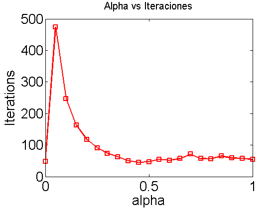
(a) Iteration number vs $\alpha$, Problem 1

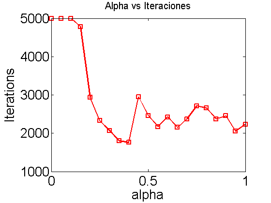
(b) Iteration number vs $\alpha$, Problem 2

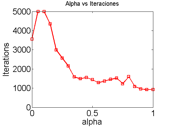
(c) Iteration number vs $\alpha$, Problem 3

Figure 1: Iteration number vs $\alpha$ with $m=100$ and $n=65$

Note that when the matrix $S$ is generated following problem 1 then the matrix $A$ has a small condition number, and when $S$ is generated following problems 2 and 3, the matrix $A$ has a big condition number, which becomes bigger as $m$ grows. In view of this, in the remainder of this subsection, we will refer to Problem 2 and Problem 3 as ill conditioned WOPP’s problems and to Problem 1 as well conditioned problems.

First of all, we perform an experiment in order to calibrate the parameters ($\alpha$,$\beta$). To make the study more tractable, we consider the direction $H_{k}$ as a convex combination of $\nabla\mathcal{F}_{1}(X_{k})$ and $\nabla\mathcal{F}_{2}(X_{k})$, that is, we put $\beta=1-\alpha$ with $\alpha\in[0,1]$. More specifically, we randomly generated one problem of each type, as explained above (Problem 1, Problem 2 and Problem 3 are generated) selecting $m=100$ and $n=65$, and each one is solved for the following alpha values: $\alpha=0:0$.$05:1$ (using Matlab notation). Figure 1 shows the curves of the iterations versus each alpha value, and for each type of problem. In this figure we see that for well-conditioned problems (Problem 1) our algorithm obtains the best result when it uses $\alpha=0.45$, converging in a time of 0.1388 seconds and with gradient norm of $NrmG=9.5410e-05$. In this plot it seems that $\alpha=0$ also produces good results because it performs very few iterations, however the algorithm gets a bad result in terms of NrmG. On the other hand, we see that for ill-conditioned problems (Problem 2,3) the algorithm 2 obtains better results when $\alpha$ approaches 1, in particular in the plot we notice that with $\alpha=1$ less iterations are done.

From this experiment and our experience testifying our algorithm for different values of $\alpha$, we note that for well-conditioned WOPP problems, our algorithm tends to perform better with values of $\alpha$ close to 0.5; whereas for WOPP ill-conditioned problems our procedure shows best results when $\alpha$ is close to 1. However, it will remain as future work to study the performance of our method for the case when the direction $H_{k}$ is taken as a linear combination instead of a convex combination of $\nabla\mathcal{F}_{1}(X_{k})$ and $\nabla\mathcal{F}_{2}(X_{k})$.

It is worth mentioning that deciding which set of parameters to use to obtain a good performance of our algorithm is not an easy task to predict, since in general these parameters will depend to a great extent on the objective function and the good or ill conditioning of the problem. A strategy to select these parameters could be to use some metaheuristic that optimize these parameters for a specific problem or application. However, based on these experiments and in our numerical experience running our algorithm, we will use for the following subsections $\beta=1-\alpha$ and we will take alpha in the set $\{0$.$5,1\}$ or some number close to 1, because this choice usually reach good results.

In the second experiment, we will test the efficiency of the non-monotone line search, by making a comparison between the Algorithm 1 and the Algorithm 2. In the Table 1 we present the results of this comparison, in this experiment we choose $(\alpha,\beta)=(1,0)$ in both algorithms. We show the minimum (min), maximum (max) and the average (mean) of the results achieved from $K=30$ simulations. According to the number of iterations a small difference in favor to algorithm 1 can be observed. However, in terms of CPU time, the dominance of algorithm 2 is overwhelming. This conclusion is also appreciated in figure 2. In view of this, for the remaining experiments we only compare our algorithm 2, which we hereafter refer as Grad-Retract, to other state of the art procedures, namely Edelman, Manton, Wen-Yin Edelman ; Manton02 ; WenYin .

Table 1: A comparative between the monotone and non-monotone case of Grad-retrac method

		Problem 1, $m=500$				Problem 2, $m=100$				Problem 3, $m=100$
		$n=20$		$n=70$		$n=10$		$n=50$		$n=10$		$n=50$
		Nitr	Time	Nitr	Time	Nitr	Time	Nitr	Time	Nitr	Time	Nitr	Time
	min	24	0.1876	33	0.6347	716	0.3561	612	1.6184	579	0.4152	578	1.6255
Algorithm 1	mean	35.23	0.3056	42.30	0.8156	1182.1	0.8397	1447.60	3.5599	1074.9	0.6466	1318	3.4910
	max	44	0.5432	49	0.9340	2920	2.0068	6902	10.802	3036	1.7612	5628	12.736
	min	22	0.0899	34	0.4564	700	0.3066	594	1.5256	630	0.3467	639	1.5509
Algorithm 2	mean	35.23	0.1574	42.97	0.5480	1193.3	0.6762	1456.10	3.0685	1060.8	0.5769	1355.90	3.1333
	max	45	0.2446	50	0.6152	2862	1.6512	7702	11.130	2322	1.3188	5084	10.349

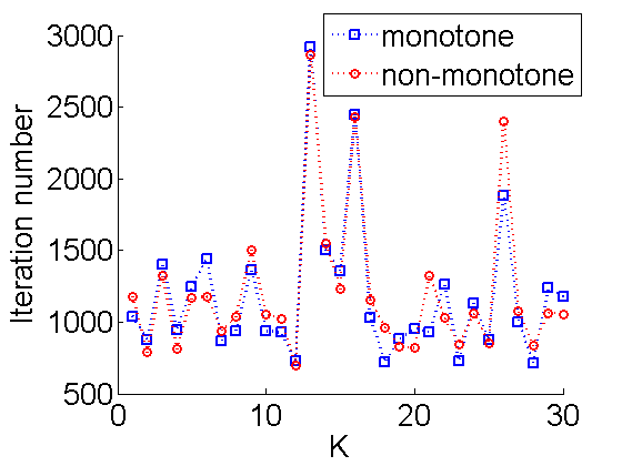
(a) Iteration number

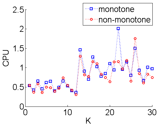
(b) CPU time in seconds

Figure 2: Algorithm 1 vs Algorithm 2, from Table 1, solving Problem 2 with $m=100$ and $n=10$

Table 2: A comparative between the Algorithm 2 and the Modified Steepest Descent Method proposed in Manton02

		Problem 1, $m=50$				Problem 2, $m=50$				Problem 3, $m=50$
		$n=20$		$n=50$		$n=20$		$n=50$		$n=20$		$n=50$
		Nitr	Time	Nitr	Time	Nitr	Time	Nitr	Time	Nitr	Time	Nitr	Time
	min	39	0.0969	179	0.9531	1851	19.811	895	9.8746	3959	69.25	2779	45.387
MSDStiefel	mean	54.70	0.1317	541.80	4.0235	4471.3	111.30	2836.9	67.527	6479.0	186.0	5611.70	156.61
	max	77	0.2208	1494	13.457	7000	239.69	7000	270.02	7000	243.05	7000	240.51
	min	22	0.0181	118	0.1676	369	0.2808	296	0.4930	653	0.4844	417	0.6182
Grad-retrac	mean	25.73	0.0221	220.40	0.3208	635.4	0.481	548.47	0.8285	1153.3	0.8561	748.70	1.0956
	max	30	0.0627	444	0.6487	1461	1.0983	1319	1.6947	2868	2.2797	1274	1.8736

In the Table 2, we compare our Grad-Retrac versus the Modified Steepest Descent Method (MSDStiefel) proposed in Manton02 . More specifically, we compare the performance of these methods solving WOPP’s. We create the matrices $A$, $C$ and $X_{0}$ as explained at the beginning of this subsection and generate the matrix $B$ randomly with their entries uniformly distributed in the range [0,1]. A total of 30 simulations were run. We see in Table 2 that the performance of our Grad-Retrac is consistently better than the performance of the algorithm proposed by Manton Manton02 , in terms of number of iterations, and CPU time. Both of the procedures solve all proposed test problems.

For all experiments presented in Tables 3-5, we compare our algorithm Grad-retrac with the methods PGST, OptStiefel proposed in Francis , WenYin respectively, and we use as tolerance $\epsilon=$ 1e-5 and as maximum number of iterations $K=8000$ for all methods. In addition, in the experiments shown in Table 3 we choose $\alpha=\beta=0.5$ (see Eq. 12), while for the experiments shown in Tables 4-5, we select: $\alpha=1$, and $\beta=0$ in the descent direction of our method. For each value to compare in these tables, we show the minimal (min), maximum (max) end the average (mean) of the results achieved from 30 simulations.

Table 3 include numerical results for well conditioned WOPP’s of different sizes. We observe from this table that all methods converge to good solutions, while our method (Grad-retrac) always performs much better than PGST and OptStiefel in terms of the CPU time, except on orthogonal group problems (see table Ex.3 and Ex.4 in table 3), where OptStiefel method shows better performance. Tables 4-5 presents the results achieved for all methods solving WOPP’s in presence of ill conditioning. In these tables, we see that Grad-retrac and OptStiefel algorithms show similar performance in most experiments, while the PGST method exhibit the worst performance in all cases examined here, however all methods achieve good solutions.

Table 3: Performance of the methods for well conditioned WOPP problems

Methods		Nitr	Time	NrmG	Fval	Feasi	Nitr	Time	NrmG	Fval	Feasi
		Ex.1: $n=500$, $p=70$, $problem=1$					Ex.2: $n=1000$, $p=100$, $problem=1$
	min	51	0.7151	2.79e-05	3.64e-12	3.40e-14	52	3.4933	9.92e-06	1.98e-13	4.21e-14
OptStiefel	mean	56.70	0.8595	7.01e-05	4.62e-11	4.14e-14	57.57	4.7568	9.15e-05	5.37e-11	5.15e-14
	max	64	1.1443	9.99e-05	1.29e-10	4.86e-14	67	7.3991	8.71e-04	2.05e-10	5.97e-14
	min	35	0.6698	1.54e-05	2.07e-12	4.71e-15	34	3.2884	2.84e-05	2.66e-12	5.83e-15
PGST	mean	37.73	0.8310	6.80e-05	4.52e-11	7.01e-15	39.27	4.8581	6.65e-05	3.44e-11	9.42e-15
	max	43	1.1251	9.82e-05	1.34e-10	9.65e-15	44	6.9226	9.56e-05	1.06e-10	1.41e-14
	min	37	0.5178	2.19e-05	1.85e-12	1.60e-14	38	2.4845	1.35e-05	6.34e-13	2.05e-14
Grad-retrac	mean	42.37	0.7121	6.86e-05	4.11e-11	3.24e-14	43.03	3.6456	6.13e-05	4.70e-11	4.08e-14
	max	48	0.9896	9.95e-05	1.38e-10	9.18e-14	47	5.5771	9.97e-05	1.51e-10	9.88e-14
		Ex.3: $n=200$, $p=200$, $problem=1$					Ex.4: $n=300$, $p=300$, $problem=1$
	min	46	0.7488	1.40e-05	2.13e-13	6.52e-14	49	2.3306	7.14e-06	8.04e-14	1.41e-14
OptStiefel	mean	51.27	1.0757	6.02e-05	7.62e-12	6.99e-14	52.93	3.4949	5.93e-05	1.12e-11	8.22e-14
	max	57	1.9995	9.87e-05	3.36e-11	7.72e-14	61	5.9582	9.99e-05	3.42e-11	9.98e-14
	min	36	1.3851	1.13e-05	1.03e-13	7.58e-15	36	4.3346	1.65e-05	9.48e-14	8.53e-15
PGST	mean	41.03	1.9658	6.20e-05	1.16e-11	1.02e-14	41.63	5.6442	6.17e-05	6.58e-12	1.03e-14
	max	47	3.4550	9.92e-05	3.87e-11	1.49e-14	46	7.2430	9.92e-05	2.54e-11	1.22e-14
	min	47	1.0511	8.47e-06	2.06e-13	5.10e-14	47	3.3157	1.51e-05	2.69e-13	6.60e-14
Grad-retrac	mean	52.80	1.5083	6.40e-05	1.18e-11	5.67e-14	53.67	4.6731	6.06e-05	9.91e-12	7.10e-14
	max	69	2.5606	9.86e-05	3.80e-11	9.93e-14	62	6.6604	9.72e-05	3.62e-11	9.43e-14
		Ex.5: $n=800$, $p=450$, $problem=1$					Ex.6: $n=1000$, $p=500$, $problem=1$
	min	56	24.126	3.50e-05	2.54e-12	2.15e-14	57	43.799	3.59e-05	2.14e-12	2.43e-14
OptStiefel	mean	63.27	33.316	7.37e-05	6.30e-11	2.23e-14	62.13	59.386	7.53e-05	5.05e-11	2.53e-14
	max	70	39.796	9.86e-05	1.36e-10	2.31e-14	74	103.86	9.71e-05	1.30e-10	2.65e-14
	min	39	23.808	3.05e-05	1.80e-12	9.57e-15	40	41.973	1.39e-05	4.45e-13	1.07e-14
PGST	mean	42.03	31.916	6.28e-05	1.88e-11	1.17e-14	42.60	57.541	5.22e-05	1.22e-11	1.23e-14
	max	44	41.976	9.80e-05	5.97e-11	1.40e-14	44	139.13	9.16e-05	3.41e-11	1.47e-14
	min	43	21.228	2.48e-05	1.07e-12	7.66e-14	41	32.012	4.21e-05	2.46e-12	7.79e-14
Grad-retrac	mean	48.73	26.162	6.63e-05	3.41e-11	8.77e-14	45.50	39.921	7.14e-05	3.98e-11	9.09e-14
	max	55	31.251	9.95e-05	1.19e-10	9.85e-14	52	58.320	9.66e-05	1.01e-10	9.96e-14

Table 4: Performance of the methods for ill conditioned WOPP problems

Methods		Nitr	Time	NrmG	Fval	Feasi	Nitr	Time	NrmG	Fval	Feasi
		Ex.7: $n=100$, $p=50$, $problem=2$					Ex.8: $n=500$, $p=20$, $problem=2$
	min	614	640	1.36e-04	3.61e-11	2.79e-15	4841	13.0517	9.32e-04	5.48e-09	1.87e-15
OptStiefel	mean	903.40	1.3854	6.26e-04	3.69e-09	3.38e-15	9827	30.1954	0.0989	0.0288	4.96e-14
	max	1348	5.4052	4.90e-03	8.42e-09	3.93e-15	15000	58.5938	2.6101	0.6063	9.84e-14
	min	556	934	1.16e-04	2.79e-11	4.93e-15	4519	25.8166	5.20e-04	6.72e-09	4.40e-15
PGST	mean	857.17	3.3145	6.89e-04	2.33e-09	6.97e-15	6849.1	46.7116	0.0159	1.11e-05	6.67e-15
	max	1440	5.6725	6.60e-03	2.62e-08	1.12e-14	11815	96.0478	0.3035	3.27e-04	9.85e-15
	min	632	653	1.40e-04	3.91e-11	1.03e-14	5176	13.0955	5.84e-04	1.38e-08	7.14e-15
Grad-retrac	mean	929.53	1.8521	3.99e-04	2.53e-09	3.02e-14	9702.8	28.5254	0.0294	0.0385	4.42e-14
	max	1925	3.6914	1.70e-03	5.76e-09	9.65e-14	15000	61.9137	0.5755	0.6063	9.91e-14
		Ex.9: $n=100$, $p=100$, $problem=2$					Ex.10: $n=200$, $p=200$, $problem=2$
	min	477	1.5892	1.17e-04	8.28e-11	5.20e-15	1088	13.841	3.37e-04	1.21e-10	1.05e-14
OptStiefel	mean	679.50	2.5212	5.60e-04	2.36e-09	5.59e-15	1611.60	20.469	3.30e-03	3.50e-08	1.10e-14
	max	1102	6.5418	1.80e-03	6.40e-09	6.19e-15	2961	37.932	2.03e-02	3.70e-07	1.16e-14
	min	543	5.4842	6.08e-05	5.82e-13	6.22e-15	1292	45	2.21e-04	1.04e-11	7.90e-15
PGST	mean	859.73	8.8871	6.16e-04	1.14e-09	8.76e-15	2138.00	77.01	3.00e-03	1.45e-08	1.02e-14
	max	1460	16.469	2.70e-03	6.01e-09	1.18e-14	3847	138	2.28e-02	1.92e-07	1.34e-14
	min	480	2.4762	1.40e-04	5.25e-11	2.40e-14	900	15.509	5.75e-04	3.80e-09	2.77e-14
Grad-retrac	mean	665.87	3.2475	1.60e-03	2.22e-09	4.10e-14	1658.80	25.174	2.10e-03	1.41e-08	6.51e-14
	max	954	4.7347	2.39e-02	9.53e-09	8.67e-14	3036	43.884	9.20e-03	3.51e-08	9.95e-14
		Ex.11: $n=200$, $p=100$, $problem=2$					Ex.12: $n=200$, $p=150$, $problem=2$
	min	1537	9.7212	4.35e-04	2.92e-09	5.64e-15	1450	14.489	3.30e-04	1.25e-09	8.06e-15
OptStiefel	mean	2291.1	14.680	1.60e-03	2.95e-08	6.37e-15	2158.40	21.815	1.90e-03	1.64e-08	8.64e-15
	max	4042	27.296	8.70e-03	2.35e-07	7.02e-15	4829	48.014	9.60e-03	3.91e-08	9.44e-15
	min	1057	13.740	2.54e-04	1.26e-09	6.21e-15	1164	26.374	2.01e-04	1.11e-10	7.11e-15
PGST	mean	2152.4	27.127	1.40e-03	1.16e-08	8.45e-15	2125.50	49.825	2.00e-03	8.35e-09	8.33e-15
	max	3180	39.891	3.50e-03	3.66e-08	1.29e-14	3337	77.428	7.30e-03	3.26e-08	1.09e-14
	min	1454	9.4400	3.93e-04	4.34e-09	1.81e-14	1263	17.645	3.11e-04	5.97e-10	2.22e-14
Grad-retrac	mean	2743.4	16.738	2.40e-03	3.45e-08	5.11e-14	2268.10	27.095	2.00e-03	2.35e-08	4.49e-14
	max	5344	32.535	3.16e-02	3.53e-07	9.82e-14	3422	38.263	1.30e-02	1.25e-07	9.56e-14

Table 5: Performance of the methods for ill conditioned WOPP problems

Methods		Nitr	Time	NrmG	Fval	Feasi	Nitr	Time	NrmG	Fval	Feasi
		Ex.13: $n=500$, $p=20$, $problem=3$					Ex.14: $n=1000$, $p=10$, $problem=3$
	min	1207	5.7719	1.32e-04	1.57e-09	3.54e-15	1206	15.846	1.69e-04	6.67e-09	7.80e-15
OptStiefel	mean	1888.00	10.739	7.08e-04	2.72e-08	3.53e-14	2299.90	29.248	9.30e-04	8.61e-08	1.89e-14
	max	3135	19.596	3.00e-03	1.24e-07	7.58e-14	3858	48.623	4.30e-03	8.44e-07	6.24e-14
	min	986	9.8174	5.33e-05	1.53e-11	3.31e-15	1288	25.262	1.43e-04	1.25e-09	2.33e-15
PGST	mean	1872.10	17.895	6.48e-04	2.86e-08	6.67e-15	2112.40	39.082	7.39e-04	3.95e-08	4.16e-15
	max	3140	30.382	4.70e-03	4.22e-07	1.03e-14	3547	64.554	3.00e-03	2.82e-07	6.44e-15
	min	1208	5.3518	9.00e-05	1.19e-09	6.31e-15	1020	13.023	1.97e-04	6.49e-09	3.37e-15
Grad-retrac	mean	1882.20	10.263	4.73e-04	2.33e-08	3.00e-14	2382.40	29.756	1.30e-03	9.70e-08	2.24e-14
	max	2897	19.609	2.40e-03	4.68e-08	9.65e-14	4268	52.634	1.21e-02	9.39e-07	8.15e-14
		Ex.15: $n=100$, $p=100$, $problem=3$					Ex.16: $n=200$, $p=200$, $problem=3$
	min	481	1.4359	1.05e-04	6.33e-11	5.25e-15	568	7.4377	1.69e-04	3.21e-11	1.06e-14
OptStiefel	mean	706.77	2.1294	8.52e-04	2.21e-09	5.55e-15	876.33	11.355	8.42e-04	3.92e-09	1.10e-14
	max	1148	3.3911	3.30e-03	7.76e-09	5.88e-15	1336	16.936	3.50e-03	1.27e-08	1.17e-14
	min	440	3.6841	6.46e-05	8.50e-13	6.79e-15	542	19.691	7.02e-05	9.63e-13	8.57e-15
PGST	mean	858.13	7.6421	5.37e-04	8.98e-10	8.93e-15	1042.10	36.663	1.30e-03	5.87e-09	1.04e-14
	max	1542	14.094	1.40e-03	7.55e-09	1.31e-14	1410	50.839	9.50e-03	1.05e-07	1.33e-14
	min	426	1.9723	2.11e-04	1.98e-10	2.23e-14	512	9.5307	1.35e-04	2.82e-11	2.81e-14
Grad-retrac	mean	680.83	2.8749	7.41e-04	2.59e-09	3.40e-14	848.77	14.911	1.00e-03	4.69e-09	5.37e-14
	max	1098	4.5067	3.40e-03	9.91e-09	7.66e-14	1290	21.070	8.80e-03	2.58e-08	9.15e-14
		Ex.17: $n=200$, $p=100$, $problem=3$					Ex.18: $n=200$, $p=150$, $problem=3$
	min	696	5.1556	1.48e-04	1.52e-10	5.19e-15	632	6.2744	1.24e-04	9.49e-11	7.99e-15
OptStiefel	mean	1176.80	10.889	1.40e-03	7.29e-09	5.63e-15	946.20	9.4612	7.73e-04	4.39e-09	8.62e-15
	max	2276	19.284	1.33e-02	4.92e-08	6.07e-15	1394	13.877	2.70e-03	1.22e-08	9.17e-15
	min	520	10.374	6.55e-05	8.36e-13	6.04e-15	630	13.926	6.84e-05	1.53e-12	7.60e-15
PGST	mean	1011.20	18.462	1.10e-03	1.38e-08	8.16e-15	967.80	21.567	4.85e-04	1.06e-09	8.74e-15
	max	1481	34.484	1.29e-02	3.58e-07	1.20e-14	1509	34.140	2.00e-03	6.82e-09	1.09e-14
	min	813	7.8483	7.77e-05	1.48e-10	1.65e-14	692	9.4317	7.39e-05	2.36e-12	2.07e-14
Grad-retrac	mean	1231.10	11.9001	1.30e-03	8.66e-09	4.29e-14	1120.50	15.026	1.20e-03	8.79e-09	4.19e-14
	max	1887	21.735	6.80e-03	7.18e-08	9.27e-14	1908	26.238	8.60e-03	8.65e-08	9.66e-14

In Figure 3, we give the convergence history of each method in the WOPP’s problems shown in the tables 3-5. More specifically, we depict the average assessments of objective function as well as the average gradient norm for Ex.5, Ex.9 and Ex.15 experiments. In these charts, we observe that in well conditioned problems (see Figure 3(a)-(b)) the method PGST converge faster than the other, but in the presence of ill conditioning, our method is faster. In addition, in all charts, OptStiefel an our method showed similar performance.

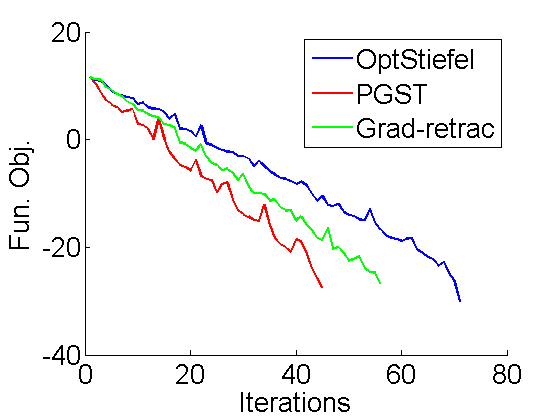
(a) Objective Function, Table 3, Ex.5

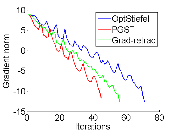
(b) Gradient norm, Table 3, Ex.5

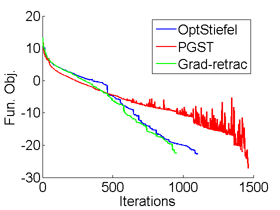
(c) Objective Function, Table 4, Ex.9

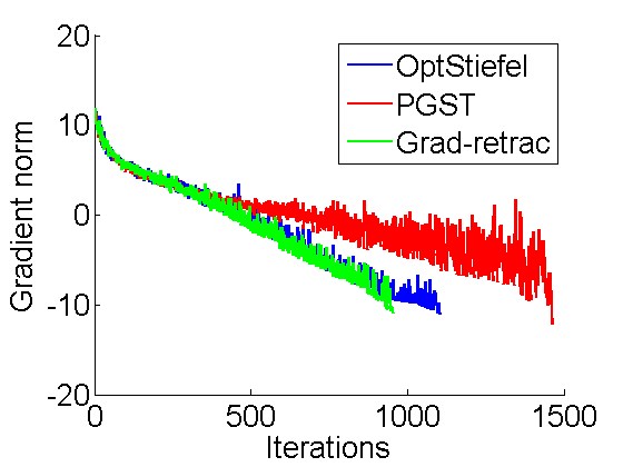
(d) Gradient norm, Table 4, Ex.9

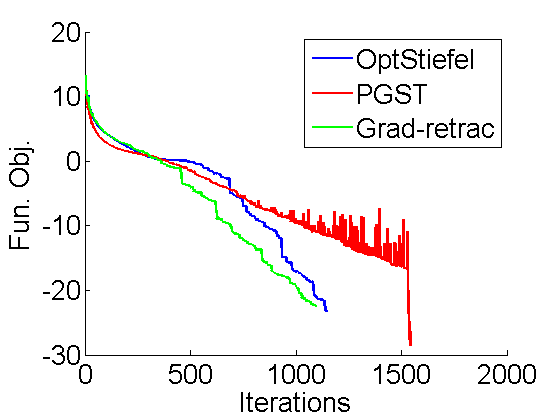
(e) Objective Function, Table 5, Ex.15

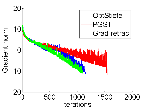
(f) Gradient norm, Table 5, Ex.15

Figure 3: Graphics assessments of the average objective function and the average gradient norm from 30 simulations. The y-axis is on a logarithmic scale.

4.3 Total energy minimization

For next experiments we consider the following total energy minimization problem:

$$\min_{X\in\mathbb{R}^{n\times k}}E_{total}(X)=\frac{1}{2}Tr[X^{\top}LX]+\frac{\mu}{4}\rho(X)^{\top}L^{{\dagger}}\rho(X)\quad s.t.\quad X^{\top}X=I_{k}$$

where $L$ is a discrete Laplacian operator, $\mu>0$ is a given constant, $\rho(X):=diag(XX^{\top})$ is the vector containing the diagonal elements of the matrix $XX^{\top}$ and $L^{{\dagger}}$ is the Moore-Penrose generalized inverse of matrix $L$. The total energy minimization problem (4.3) is a simplified version of the HartreeFock (HF) total energy minimization problem and the Kohn-Sham (KS) total energy minimization problem in electronic structure calculations (see for instance martin2004electronic ; ostlund1996modern ; yang2006constrained ; yang2007trust ). The first order necessary conditions for the total energy minimization problem (4.3) are given by:

$$H(X)X-X\Lambda = 0$$

$$X^{\top}X = I_{k},$$

where the diagonal matrix $\Lambda$ contains the $k$ smallest eigenvalues of the symmetric matrix $H(X):=L+\mu Diag(L^{{\dagger}}\rho(X))$. The symbol $Diag(x)$ is a diagonal matrix with a vector $x$ on its diagonal.

For examples 6.1-6.4 below taken from ZhaoBai , we repeat our experiments over 100 different starting points, moreover, we use a tolerance of $\epsilon=$ 1e-4 and a maximum number of iterations $K=1000$. To show the effectiveness of our method over the problem (4.3), we report the numerical results for Examples 6.1-6.4 with different choices of $n$, $k$, and $\mu$, and we compare our method with the Steepest Descent method (Steep-Dest), Trust-Region method (Trust-Reg) and Conjugate Gradient method (Conj-Grad) from “manopt” tool­box.

Example 6.1 ZhaoBai : We consider the nonlinear eigenvalue problem for different choices of $n$; $k$; $\mu$: (a) $n=2$; $k=1$; $\mu=3$; (b) $n=10$; $k=2$; $\mu=0.6$; (c) $n=100$; $k=10$; $\mu=0.005$; (d) $n=100$; $k=4$; $\mu=0.001$.

Example 6.2 ZhaoBai : We consider the nonlinear eigenvalue problem for different choices of $n$; $k$; $\mu$: (a) $n=2$; $k=1$; $\mu=9$; (b) $n=10$; $k=2$; $\mu=3$; (c) $n=100$; $k=10$; $\mu=1$; (d) $n=100$; $k=4$; $\mu=2$.

Example 6.3 ZhaoBai : We consider the nonlinear eigenvalue problem for $k=10$; $\mu=1$, and varying $n=200,400,800,1000$.

Example 6.4 ZhaoBai : We consider the nonlinear eigenvalue problem for $n=100$ and $k=20$ and varying $\mu$.

In all these experiments, the $L$ matrix in the problem (4.3) is constructed as the one-dimensional discrete Laplacian with $2$ on the diagonal and $-1$ on the sub- and sup-diagonals. Furthermore, for all these experiments we select: $\alpha=0.7$, and $\beta=0.3$ in the descent direction of our method.

The results for the Example 6.1 and Example 6.2 are shown in Tables 6-7. We see from these tables that our method (Grad-retrac) is more efficient than the other methods from “manopt” tool­box in terms of CPU time. Table 8 gives numerical results for Example 6.3. We see from Table 8 that in almost all cases, our method is more efficient than the other in terms of CPU time. Only in experiments Ex.11 and Ex.12 (see Table 8), the Conjugate Gradient method from “manopt” library gets better performance than our method slightly. In addition, all algorithms take longer to converge as it increases the value of $n$, nevertheless, when the problems are larger size, the increase in the convergence time of the Conj-Grad and Grad-retrac methods is much less than the of the other methods.

Table 6: Numerical results for Example 6.1

	Ex.1: $(n,k,\mu)=(2,1,3)$					Ex.2: $(n,k,\mu)=(10,2,0.6)$
Methods	Nitr	Time	NrmG	Fval	Feasi	Nitr	Time	NrmG	Fval	Feasi
Trust-Reg	4.48	0.0141	1.19e-04	0.8750	1.95e-16	7.79	0.0264	1.51e-04	0.8495	5.27e-16
Steep-Dest	6.52	0.0160	4.22e-04	0.8750	2.00e-16	23.54	0.0519	5.51e-04	0.8495	5.12e-16
Conj-Grad	5.62	0.0126	7.40e-03	0.8752	1.94e-16	17.08	0.0309	4.60e-03	0.8513	5.31e-16
Grad-retrac	5.72	0.0032	1.56e-05	0.8750	2.96e-15	22.11	0.0087	6.47e-05	0.8495	1.21e-14
	Ex.3: $(n,k,\mu)=(100,10,0.005)$					Ex.4: $(n,k,\mu)=(100,4,0.001)$
Trust-Reg	13.00	0.1524	1.81e-04	1.0547	2.58e-15	11.80	0.1632	3.05e-04	5.02e-02	1.37e-15
Steep-Dest	535.71	2.1547	3.58e-04	1.0548	1.99e-15	930.94	3.1733	2.46e-04	5.02e-02	1.32e-15
Conj-Grad	69.32	0.1897	8.14e-04	1.0548	2.72e-15	80.46	0.1901	8.92e-04	5.03e-02	1.45e-15
Grad-retrac	105.29	0.0782	7.46e-05	1.0547	2.52e-14	129.09	0.0711	8.03e-05	5.02e-02	2.55e-14

Table 7: Numerical results for Example 6.2

	Ex.5: $(n,k,\mu)=(2,1,9)$					Ex.6: $(n,k,\mu)=(10,2,3)$
Methods	Nitr	Time	NrmG	Fval	Feasi	Nitr	Time	NrmG	Fval	Feasi
Trust-Reg	3.53	0.0090	1.07e-04	1.9350	2.00e-16	8.63	0.0260	2.33e-04	2.5046	5.78e-16
Steep-Desct	7.15	0.0172	4.22e-04	1.6250	2.09e-16	17.76	0.0392	5.41e-04	2.5046	5.16e-16
Conj-Grad	4.75	0.0106	5.23e-02	1.8380	2.25e-16	15.69	0.0284	7.12e-04	2.5046	5.50e-16
Grad-retrac	5.47	0.0028	1.37e-05	1.9150	3.24e-15	19.35	0.0077	5.92e-05	2.5046	1.92e-14
	Ex.7: $(n,k,\mu)=(100,10,1)$					Ex.8: $(n,k,\mu)=(100,4,2)$
Trust-Reg	19.77	0.1622	5.53e-04	35.7086	2.76e-15	12.10	0.0601	2.66e-04	7.7005	1.42e-15
Steep-Desct	149.89	0.5982	4.33e-04	35.7086	1.96e-15	42.33	0.1260	4.65e-04	7.7005	1.48e-15
Conj-Grad	44.03	0.1134	8.10e-04	35.7086	3.04e-15	25.76	0.0558	7.00e-04	7.7005	1.48e-15
Grad-retrac	65.33	0.0464	7.47e-05	35.7086	2.74e-14	36.77	0.0200	6.58e-05	7.7005	1.85e-14

Table 9 lists numerical results for Example 6.4. In this table, we note that our method gets its best performance when it used the smaller size of $\mu$, we also observe that our method is more efficient than the other in all of the experiments list in this table.

Table 8: Numerical results for Example 6.3

	Ex.9: $(n,k,\mu)=(200,10,1)$					Ex.10: $(n,k,\mu)=(400,10,1)$
Methods	Nitr	Time	NrmG	Fval	Feasi	Nitr	Time	NrmG	Fval	Feasi
Trust-Reg	20.13	0.2146	5.28e-04	35.7086	2.90e-15	21.29	0.6052	5.42e-04	35.7086	3.05e-15
Steep-Dest	156.38	0.7624	3.70e-04	35.7086	2.07e-15	155.39	1.1328	3.92e-04	35.7086	2.19e-15
Conj-Grad	45.01	0.1362	7.85e-04	35.7086	3.07e-15	46.74	0.2308	7.92e-04	35.7086	3.30e-15
Grad-retrac	65.38	0.0654	7.48e-05	35.7086	2.23e-14	67.27	0.1644	7.17e-05	35.7086	2.77e-14
	Ex.11: $(n,k,\mu)=(800,10,1)$					Ex.12: $(n,k,\mu)=(1000,10,1)$
Trust-Reg	21.23	2.3096	5.50e-04	35.7086	3.21e-15	21.78	2.9471	5.67e-04	35.7086	3.40e-15
Steep-Dest	158.52	2.6007	3.71e-04	35.7086	2.78e-15	157.96	2.7528	4.17e-04	35.7086	3.48e-15
Conj-Grad	47.52	0.5641	8.14e-04	35.7086	3.77e-15	47.53	0.6426	8.27e-04	35.7086	3.94e-15
Grad-retrac	67.13	0.5777	7.55e-05	35.7086	3.41e-14	68.16	0.7171	7.52e-05	35.7086	2.94e-14

Table 9: Numerical results for Example 6.4

	Ex.13: $(n,k,\mu)=(100,20,0.0001)$					Ex.14: $(n,k,\mu)=(100,20,0.001)$
Methods	Nitr	Time	NrmG	Fval	Feasi	Nitr	Time	NrmG	Fval	Feasi
Trust-Reg	11.27	0.1060	2.56e-04	1.4484	4.34e-15	11.17	0.1061	3.09e-04	2.2066	4.39e-15
Steep-Dest	253.37	1.3326	3.77e-04	1.4484	2.83e-15	238.17	1.2122	4.09e-04	2.2066	2.60e-15
Conj-Grad	48.24	0.1554	8.46e-04	1.4484	5.44e-15	48.80	0.1585	8.72e-04	2.2066	5.37e-15
Grad-retrac	74.24	0.0776	7.57e-05	1.4484	3.14e-14	73.26	0.0784	7.49e-05	2.2066	2.56e-14
	Ex.15: $(n,k,\mu)=(100,20,0.01)$					Ex.16: $(n,k,\mu)=(100,20,0.1)$
Trust-Reg	15.34	0.2084	3.87e-04	7.8706	4.19e-15	21.33	0.3239	6.15e-04	33.7574	5.01e-15
Steep-Dest	391.23	2.2931	2.62e-04	7.8706	2.60e-15	448.39	3.7625	2.43e-04	33.7574	2.54e-15
Conj-Grad	60.44	0.2243	8.42e-04	7.8706	5.62e-15	64.84	0.3026	8.66e-04	33.7574	5.85e-15
Grad-retrac	87.43	0.1070	7.81e-05	7.8706	4.09e-14	99.48	0.1463	8.01e-05	33.7574	4.02e-14
	Ex.17: $(n,k,\mu)=(100,20,1)$					Ex.18: $(n,k,\mu)=(100,20,20)$
Trust-Reg	25.30	0.2863	5.99e-04	2.11e+02	5.48e-15	34.15	0.3929	5.17e-04	3.87e+03	5.84e-15
Steep-Dest	555.11	3.6971	3.04e-04	2.11e+02	2.67e-15	1797.70	18.3231	3.90e-04	3.87e+03	2.73e-15
Conj-Grad	81.45	0.2726	8.57e-04	2.11e+02	5.46e-15	153.16	0.5131	8.63e-04	3.87e+03	3.50e-15
Grad-retrac	116.49	0.1222	1.35e-04	2.11e+02	2.62e-14	160.62	0.1661	2.70e-03	3.87e+03	2.55e-14
	Ex.19: $(n,k,\mu)=(100,20,40)$					Ex.20: $(n,k,\mu)=(100,20,80)$
Trust-Reg	37.46	0.5130	5.90e-04	7.72e+03	6.14e-15	41.35	0.5403	6.63e-04	1.54e+04	6.25e-15
Steep-Dest	2162.70	21.7257	3.67e-04	7.72e+03	2.69e-15	3585.60	37.5829	3.61e-04	1.54e+04	2.55e-15
Conj-Grad	179.83	0.7251	8.63e-04	7.72e+03	3.17e-15	212.05	0.8118	8.55e-04	1.54e+04	2.97e-15
Grad-retrac	173.46	0.2159	5.60e-03	7.72e+03	2.77e-14	192.18	0.2208	1.25e-02	1.54e+04	2.76e-14

4.4 Linear eigenvalue problem

Given a symmetric matrix $A\in\mathbb{R}^{n\times n}$ and let $\lambda_{1}\geq\ldots\geq\lambda_{n}$ be the eigenvalues of $A$. The $p$-largest eigenvalue problem can be formulated as:

$$\sum_{i=1}^{p}\lambda_{i}:=\max_{X\in\mathbb{R}^{n\times p}}Tr[X^{\top}AX]\quad s.t.\quad X^{\top}X=I$$

In this subsection, we compared Algorithm 2 with the Sgmin algorithm proposed in Edelman and the OptStiefel proposed in WenYin . In this case, $\nabla\mathcal{F}_{1}=\nabla\mathcal{F}_{2}$, so, our direction coincide with Manton’s direction. In all experiments presented in this subsection, we generate the matrix $A$ as follows: $A=\overline{A}^{\top}\overline{A}$, where $\overline{A}\in\mathbb{R}^{n\times n}$ is a matrix whose elements are sampled from the standard Gaussian distribution. The tables 10-11 shows the average (mean) of the results achieved for each value to compare from 100 simulations, in addition, we used 1000 by the maximum number of iterations and $\epsilon=$ 1e-5 as tolerance for each algorithm. For all methods to compare, we use the four stop criteria presented in subsection 4.1 In this tables, Error denotes the relative error between the objective values given by eigs function of Matlab and the objective values obtain by each algorithm, i.e.

$$Error:=\frac{|\sum_{i=1}^{p}\lambda_{i}^{eig}-Tr[X_{est}^{\top}AX_{est}]|}{|Tr[X_{est}^{\top}AX_{est}]|}$$

where $\lambda_{i}^{eig}$ is the $i$-largest eigenvalue of $A$ calculated using the eig function of Matlab, and $X_{est}$ denotes the estimated local optima for each algorithm.

The results corresponding to varying $p$ but fixed $n=1000$ are presented in Table 10, from these results we can observe that OptStiefel and our Grad-retrac are much more efficient methods that Sgmin. Moreover, we observe that OptStiefel and Grad-retrac show almost the same performance, we also see that when $p$ grows, our method converges faster OptStiefel in terms of CPU time (see Table 10 with $p=100$ and $p=200$). The second test compares the algorithms to a fixed value of $p$ and varying $n$, the numerical results of this test are presented in Table 11, in this table we note that OptStiefel and Grad-retrac algorithms showed similar performance, while the method Sgmin shows poor performance.

Table 10: Eigenvalues on randomly generated dense matrices for fixed n = 1000 and varying p.

p	1	5	10	50	100	200
Sgmin
Nitr	37.91	61.19	77.33	111.39	124.65	176.82
Time	22.9206	54.318	79.3343	173.187	306.8699	1128.10
Nfe	69.39	95.67	114.03	153.91	169.93	226.69
Fval	3.97e+03	1.94e+04	3.81e+04	1.72e+05	3.14e+05	5.36e+05
NrmG	9.67e-04	2.40e-03	3.50e-03	7.70e-03	1.04e-02	1.15e-02
Feasi	9.88e-17	4.61e-16	7.20e-16	2.55e-15	4.33e-15	7.74e-15
Error	9.63e-13	2.09e-12	3.73e-12	6.98e-12	9.21e-12	1.07e-11
OptStiefel
Nitr	102.7	125.86	142.69	185.84	213.33	439.94
Time	0.1595	0.4831	0.75	2.2888	5.4833	34.9373
Nfe	106.33	130.48	148.53	194.1	223.61	462.64
Fval	3.97e+03	1.94e+04	3.81e+04	1.72e+05	3.14e+05	5.36e+05
NrmG	5.73e-04	1.40e-03	1.80e-03	3.90e-03	4.10e-03	1.12e-02
Feasi	2.12e-15	7.07e-17	3.01e-15	8.31e-15	1.20e-14	1.76e-14
Error	3.98e-13	8.40e-13	1.23e-12	2.03e-12	2.47e-12	3.36e-12
Grad-retrac
Nitr	100.16	126.39	141.73	180.38	213.31	257.51
Time	0.159	0.5138	0.7661	2.413	5.4744	20.509
Nfe	102.92	130.26	146.85	187.22	223.75	271.49
Fval	3.97e+03	1.94e+04	3.81e+04	1.72e+05	3.14e+05	5.36e+05
NrmG	4.95e-04	1.50e-03	2.50e-03	3.80e-03	4.50e-03	4.80e-03
Feasi	8.66e-15	1.98e-14	2.07e-14	3.37e-14	3.78e-14	4.66e-14
Error	5.04e-13	7.46e-13	1.30e-12	2.36e-12	2.22e-12	3.96e-12

Table 11: Eigenvalues on randomly generated dense matrices for fixed p = 6 and varying n.

n	50	100	600	1000	2000	3000
Sgmin
Nitr	23.61	28.43	51.8	66.26	86.87	94.30
Time	0.4731	0.8486	19.4008	63.3436	331.3508	773.992
Nfe	51.1	58.26	85.44	101.97	124.95	133.37
Fval	9.14e+02	2.04e+03	1.37e+04	2.32e+04	4.70e+04	7.08e+04
NrmG	6.53e-05	1.78e-04	1.50e-03	2.70e-03	5.60e-03	8.50e-03
Feasi	4.14e-16	4.27e-16	4.74e-16	5.22e-16	5.71e-16	5.92e-16
Error	2.13e-13	3.88e-13	2.00e-12	2.51e-12	4.50e-12	5.16e-12
OptStiefel
Nitr	63.07	70.33	114.05	135	169.01	188.73
Time	0.0121	0.0192	0.1829	0.6169	3.2749	7.3311
Nfe	66.83	74.18	118.24	139.91	179.01	200.16
Fval	9.14e+02	2.04e+03	1.37e+04	2.32e+04	4.70e+04	7.08e+04
NrmG	2.50e-05	8.13e-05	8.86e-04	1.40e-03	3.60e-03	4.90e-03
Feasi	6.58e-16	8.05e-16	1.70e-15	2.24e-15	3.29e-15	3.87e-15
Error	3.25e-14	6.82e-14	5.45e-13	8.40e-13	2.21e-12	2.61e-12
Grad-retrac
Nitr	62.02	69.29	116.77	136.82	167.55	187.77
Time	0.0171	0.0276	0.2073	0.6494	3.2812	7.3301
Nfe	63.26	70.53	119.84	141.45	176.35	197.70
Fval	9.14e+02	2.04e+03	1.37e+04	2.32e+04	4.70e+04	7.08e+04
NrmG	2.43e-05	8.92e-05	8.20e-04	1.70e-03	3.10e-03	4.10e-03
Feasi	1.77e-14	1.89e-14	1.50e-14	1.69e-14	1.81e-14	2.12e-14
Error	2.96e-14	6.89e-14	5.21e-13	8.06e-13	1.59e-12	1.94e-12

5 Conclusion

In this article we study a feasible approach to deal with orthogonally constrained optimization problems. Our algorithm implements the non-monotone Barzilai-Borwein line search on a mixed gradient based search direction. The feasibility at each iteration is guaranteed by projecting each updated point, which is in the current tangent space, onto the Stiefel manifold, through SVD’s decomposition. The mixture is controlled by the coefficients $\alpha$ and $\beta$, associated to $\nabla\mathcal{F}_{1}(X_{k})$ and $\nabla\mathcal{F}_{2}(X_{k})$ respectively. When $\alpha=1$ and $\beta=0$, the obtained direction coincides with Manton’s direction, and the difference to these method is just the implementation of BB-line search instead of Armijo’s.

Our Grad-retract algorithm is numerically compared to other state-of-the art algorithms, in a variety of test problems, achieving clear advantages in many cases.

- (1) Absil, P. A., Mahony, R. and Sepulchre, R. (2009) Optimization Algorithms on Matrix Manifolds. Princeton University Press.
- (2) Absil, P. A. and Malick, J. (2012) Projection-like retractions on matrix manifolds. SIAM Journal on Optimization, 22(1), 135-158.
- (3) Barzilai, J. and Borwein, J. M. (1988) Two-point step size gradient methods. IMA Journal of Numerical Analysis, 8(1), 141-148.
- (4) Dai, Y.H. and Fletcher R. (2005) Projected Barzilai-Borwein methods for large-scale box-constrained quadratic programming. Numerische Mathematik, 100(1), 21-47.
- (5) D’Aspremont, A., Ei Ghaoui, L., Jordan, M.I. and Lanckriet, G.R. (2007) A direct formulation for sparse PCA using semidefinite programming. SIAM Review 49(3), 434-448.
- (6) Edelman, A., Arias, T.A. and Smith, S.T. (1998) The geometry of algorithms with orthogonality constraints. SIAM Journal on Matrix Analysis and Applications 20(2), 303-353.
- (7) Eldén, L. and Park, H. (1999) A procrustes problem on the Stiefel manifold. Numerische Mathematik 82(4), 599-619.
- (8) Francisco, J.B. and Martini, T. (2014) Spectral projected gradient method for the procrustes problem. TEMA (So Carlos), 15(1), 83-96.
- (9) Golub, G.H. and Van Loan, C.F. (2012) Matrix Computations. (Vol. 3), JHU Press.
- (10) Grubiić I. and Pietersz, R. (2007) Efficient rank reduction of correlation matrices. Linear Algebra and its Applications, 422(2), 629-653.
- (11) Joho, M. and Mathis, H. (2002) Joint diagonalization of correlation matrices by using gradient methods with application to blind signal separation. In: Sensor Array and Multichannel Signal Processing Workshop Proceedings, pp. 273-277. IEEE.
- (12) Journée, M., Nesterov, Y., Richtárik, P. and Sepulchre, R. (2010) Generalized power method for sparse principal component analysis. Journal of Machine Learning Research, 11(Feb), 517-553.
- (13) Kokiopoulou, E., Chen, J. and Saad, Y. (2011) Trace optimization and eigenproblems in dimension reduction methods. Numerical Linear Algebra with Applications, Volume 18, Issue 3, pages 565-602.
- (14) Lai, R. and Osher, S. (2014) A splitting method for orthogonality constrained problems. Journal of Scientific Computing, 58(2), 431-449.
- (15) Liu, Y.F., Dai, Y.H. and Luo, Z.Q. (2011) On the complexity of leakage interference minimization for interference alignment. IEEE 12th International Workshop on Signal Processing Advances in Wireless Communications, pp. 471-475.
- (16) Manton, J. H. (2002) Optimization algorithms exploiting unitary constraints. IEEE Transactions on Signal Processing, 50(3), 635-650.
- (17) Martin, R. M. (2004) Electronic Structure: Basic Theory and Practical Methods. Cambridge university press.
- (18) Nocedal, J. and Wright, S. J. (2006) Numerical Optimization, Springer Series in Operations Research and Financial Engineering. Springer, New York, second ed.
- (19) Pietersz, R. and Groenen, P.J. (2004) Rank reduction of correlation matrices by majorization. Quantitative Finance 4(6), 649-662.
- (20) Raydan M. (1997) The Barzilai and Borwein gradient method for the large scale unconstrained minimization problem. SIAM Journal on Optimization, 7(1), 26-33.
- (21) Rebonato, R. and Jckel, P. (1999) The most general methodology to creating a valid correlation matrix for risk manage-ment and option pricing purposes. Journal of Risk 2, 17-27.
- (22) Saad, Y. (1992) Numerical Methods for Large Eigenvalue Problems. (Vol. 158), Manchester: Manchester University Press.
- (23) Schnemann, P.H., A generalized solution of the orthogonal Procrustes problem. Psychometrika 31(1), 1-10.
- (24) Szabo, A. and Ostlund, N. S. (1966) Modern Quantum Chemistry: Introduction to Advanced Electronic Structure Theory. Courier Corporation.
- (25) Theis, F., Cason, T. and Absil, P.A. (2009) Soft dimension reduction for ICA by joint diagonalization on the stiefel manifold. In: International Conference on Independent Component Analysis and Signal Separation (pp. 354-361). Springer Berlin Heidelberg.
- (26) Wen, Z., Yang, C., Liu, X. and Zhang, Y. (2016) Trace-penalty minimization for large-scale eigenspace computation. Journal of Scientific Computing, 66(3), 1175-1203.
- (27) Wen, Z.W. and Yin, W.T. (2013) A feasible method for optimization with orthogonality constraints. Mathematical Programming, 142(1-2), 397-434.
- (28) Yang, C., Meza, J. C. and Wang, L. W. (2006) A constrained optimization algorithm for total energy minimization in electronic structure calculations. Journal of Computational Physics, vol. 217, no 2, p. 709-721.
- (29) Yang, C., Meza, J. C. and Wang, L. W. (2007) A trust region direct constrained minimization algorithm for the Kohn-Sham equation. SIAM Journal on Scientific Computing, vol. 29, no 5, p. 1854-1875.
- (30) Yang, C., Meza, J. C., Lee, B. and Wang, L.W. (2009) KSSOLV - a Matlab toolbox for solving the Kohn-Sham equations. ACM Transactions on Mathematical Software 36, 1-35.
- (31) Zhang, H. and Hager, W. (2004) A nonmonotone line search technique and its application to unconstrained optimization. SIAM Journal on Optimization, 14(4), 1043-1056.
- (32) Zhao, Z., Bai, Z. J. and Jin, X. Q. (2015) A Riemannian Newton algorithm for nonlinear eigenvalue problems. SIAM Journal on Matrix Analysis and Applications, 36(2), 752-774. ISO 690.
- (33) Zou, H., Hastie, T., and Tibshirani, R. (2006) Sparse principal component analysis. Journal of Computational and Graphical Statistics 15(2), 265-286.