Anisotropic deformations of spatially open cosmology in massive gravity theory

Abstract

We study anisotropic deformations of the spatially open homogeneous and isotropic cosmology in the ghost free massive gravity theory with flat reference metric. We find that if the initial perturbations are not too strong then the physical metric relaxes back to the isotropic de Sitter state. However, the dumping of the anisotropies is achieved at the expense of exciting the Stueckelberg fields in such a way that the reference metric changes and does not share anymore with the physical metric the same rotational and translational symmetries. As a result, the universe evolves towards a fixed point which does not coincide with the original solution, but for which the physical metric is still de Sitter. If the initial perturbation is strong, then its evolution generically leads to a singular anisotropic state or, for some parameter values, to a decay into flat spacetime. We also present an infinite dimensional family of new homogeneous and isotropic cosmologies in the theory.

1 Introduction

The main motivation for studying theories with massive gravitons is the fact that they offer an explanation for the current universe acceleration [1, 2]. Specifically, the ghost-free massive gravity theory [3] admits self-accelerating cosmological solutions with the Hubble rate proportional to the graviton mass.

This theory actually admits infinitely many such vacuum solutions. For all of them the physical metric is de Sitter and the reference metric is flat but the Stueckelberg scalars are different for different solutions. There is only one special solution for which the physical and reference metrics share the same translational and rotational Killing symmetries and can be simultaneously diagonalised and put to the standard Friedmann-Lema$\hat{\mbox{\i}}$tre-Robertson-Walker (FLRW) form [4]. In what follows we shall call this solution type I FLRW. For all other solutions the two metrics share a smaller amount of symmetries and cannot be simultaneously brought to the FLRW form [5, 6, 7, 8, 9, 10]; we shall call them type II FLRW.

Since both metrics of type I FLRW solution are simultaneously FLRW, the correlation functions of their perturbations are expected to be statistically homogeneous and isotropic. On the other hand, the correlation functions of perturbations of type II FLRW solutions are expected to develop statistical inhomogeneity or/and anisotropy, even though each of the two unperturbed metrics is perfectly FLRW. For these reasons the type I FLRW solution has attracted more attention.

At the same time, this solution exhibits some peculiar features. First, it is manifestly type I FLRW only in the spatially open slicing, but when its physical metric is expressed in the spatially flat slicing, its reference metric looks inhomogeneous. Secondly, its massive degrees of freedom are not seen within the linear perturbation theory but only at the non-linear level [11]. This means that the solution shows strong coupling, which indicates that the classical description may break down. Finally, there are indications that the solution may show ghost [12, 13]. These features, especially the latter one, have been viewed as obstacles for building realistic cosmology and served a strong motivation for searching for extensions and/or modifications of the original dRGT massive gravity theory. Examples of such modified models that allow for stable self-accelerating de Sitter cosmology include bigravity [14, 15, 16], extensions [17, 18, 19] of the quasidilaton theory [20, 21], generalized massive gravity [22], minimal theory of massive gravity [23, 24, 25], and so on.

At the same time, one should emphasise that Refs.[12, 13] actually present the stability analysis of a different solution obtained within a different theory and not of the original solution of Ref.[4]. Specifically, Refs.[12, 13] consider massive gravity with de Sitter and not flat reference metric, because in such a theory there exists a type I FLRW solution with flat spatial sections whose perturbations are relatively easy to study. This solution admits anisotropic generalisations within the Bianchi I class [26], whose analysis has revealed nonlinear ghost instability [12, 13]. Now, since this type I FLRW solution of the modified theory is somewhat similar to the original type I FLRW solution of Ref.[4], this suggests that the latter may have ghost too. However, so far nobody has confirmed or disproved this conjecture by directly studying non-linear deformations of type I FLRW solution of Ref.[4]. Therefore, strictly speaking, the analysis of stability of this solution with a possible detection of ghosts or proving their absence remains an open problem.

In what follows, as a first step towards our understanding of this problem, we shall present our analysis of fully non-linear anisotropic (but homogeneous) deformations of the original type I FLRW solution within the Bianchi V class. In brief, we find that when perturbed, this solution cannot relax back to itself, hence it is unstable. However, if the initial perturbation is not very strong, then the physical de Sitter geometry does relax back to itself and the anisotropies get damped. During the relaxation the Stueckelberg fields change in such a way that the reference metric does not share anymore with the physical metric the same rotational and translational symmetries. As a result, type I FLRW solution evolves towards type II FLRW late time attractor. This behavior is similar to what was found in [26] in the massive gravity with de Sitter reference metric. Our analysis does not include perturbations beyond the Bianchi V ansatz and thus the issue of ghosts and stability of type II FLRW solutions remain open. (See [12, 13] for the analysis of stability of type II FLRW solutions in the theory with de Sitter reference metric.) We also study strong initial perturbations and find that their evolution generically leads to a singular state where one of the scale factors vanishes. However, for some parameter values it may lead to a decay into flat spacetime.

The rest of the text is organised as follows. In the following two Sections we introduce the dRGT ghost free massive gravity theory and describe its known homogeneous and isotropic cosmological solutions. Section 4 presents the field equations for the anisotropic Bianchi V metrics. In Section 5 these equations are analysed for vanishing anisotropies, which yields the known type I but also new type II FLRW solutions. In Section 6 small anisotropies are studied. Since the first order deviations from type I FLRW solution are trivial (strong coupling), we expand up to the second order and find that the resulting non-linear equations do not admit solutions which tend to zero in the long run. Hence, when perturbed, type I FLRW solution cannot relax to itself. We also analyse linear perturbations around type II FLRW solutions and find that they all vanish at late times. In Sections 7.1, 7.2, and 8 the anisotropic solutions are studied at the fully non-linear level. Section 7.1 contains the analysis of constraints needed to put the equations into the form suitable for numerical integration, the equations themselves are displayed in Section 7.2, while their numerical solutions are described in Section 8. A brief summary of our results is given in Section 9. The special isotropic solutions are considered in Appendix A, while Appendix B presents the generalisation of type II FLRW solutions studied in the text to an infinite dimensional family of new homogeneous and isotropic dRGT cosmologies.

We use units in which the length scale is the inverse graviton mass.

2 The dRGT massive gravity

The theory is defined on a four-dimensional spacetime manifold endowed with two metrics, the physical one $g_{\mu\nu}$ and the flat reference metric $f_{\mu\nu}=\eta_{AB}\partial_{\mu}X^{A}\partial_{\nu}X^{B}$ with $\eta_{AB}={\rm diag}[-1,1,1,1]$. The scalars $X^{A}(x)$ are sometimes called Stueckelberg fields. The theory is defined by the action

$$S=\frac{M_{\rm Pl}^{2}}{m^{2}}\int\,\left(\frac{1}{2}\,R({g})-{\cal U}\right)\sqrt{-g}\,d^{4}x\,,$$ (2.1)

where the metrics and all coordinates are assumed to be dimensionless, the length scale being the inverse graviton mass $1/m$. The interaction between the two metrics is determined by the tensor $\gamma^{\mu}_{\leavevmode\nobreak\ \nu}$ defined by the relation

$$(\gamma^{2})^{\mu}_{\leavevmode\nobreak\ \nu}\equiv\gamma^{\mu}_{\leavevmode\nobreak\ \alpha}\gamma^{\alpha}_{\leavevmode\nobreak\ \nu}={g}^{\mu\alpha}{f}_{\alpha\nu}.$$ (2.2)

Hence, using the hat to denote matrices, one has $\hat{\gamma}=\sqrt{\hat{g}^{-1}\hat{f}}$. If $\lambda_{A}$ are eigenvalues of $\hat{\gamma}$ then the interaction potential is

$${\cal U}=b_{0}+\sum_{n=1}^{3}b_{k}\,{\cal U}_{k}\,,$$ (2.3)

where $b_{0},b_{k}$ are parameters and ${\cal U}_{k}$ are defined by (with $[\gamma]\equiv{\rm tr}(\hat{\gamma})$ and $[\gamma^{k}]\equiv{\rm tr}(\hat{\gamma}^{k})$)

$${\cal U}_{1} = \sum_{A}\lambda_{A}=[\gamma],\leavevmode\nobreak\ \leavevmode\nobreak\ \leavevmode\nobreak\ \leavevmode\nobreak\ \leavevmode\nobreak\ {\cal U}_{2}=\sum_{A<B}\lambda_{A}\lambda_{B}=\frac{1}{2!}([\gamma]^{2}-[\gamma^{2}]),$$

$${\cal U}_{3} = \sum_{A<B<C}\lambda_{A}\lambda_{B}\lambda_{C}=\frac{1}{3!}([\gamma]^{3}-3[\gamma][\gamma^{2}]+2[\gamma^{3}]).$$ (2.4)

The metric $g_{\mu\nu}$ and the scalars $X^{A}$ are the variables of the theory. Varying the action with respect to $g_{\mu\nu}$ gives the Einstein equations

$$G_{\mu\nu}=T_{\mu\nu}$$ (2.5)

with the energy-momentum tensor

$$T^{\mu}_{\leavevmode\nobreak\ \nu} = \{b_{1}+b_{2}\,{\cal U}_{1}+b_{3}\,{\cal U}_{2}\}\gamma^{\mu}_{\leavevmode\nobreak\ \nu}-\{b_{2}+b_{3}\,{\cal U}_{1}\}(\gamma^{2})^{\mu}_{\leavevmode\nobreak\ \nu}+b_{3}(\gamma^{3})^{\mu}_{\leavevmode\nobreak\ \nu}-{\cal U}\,\delta^{\mu}_{\nu}\,.\leavevmode\nobreak\ \leavevmode\nobreak\ \leavevmode\nobreak\ \leavevmode\nobreak\$$ (2.6)

Varying with respect to the Stueckelberg fields $X^{A}$ gives the conservation conditions

$${\nabla}_{\mu}T^{\mu}_{\leavevmode\nobreak\ \nu}=0.$$ (2.7)

These equations also follow from the Bianchi identities for the Einstein equations.

3 Homogeneous and isotropic cosmologies: a review

Equations (2.5) admit a cosmological solution whose physical and reference metrics are simultaneously homogeneous and isotropic [4],

$$ds_{g}^{2}=-dt^{2}+{\bf a}^{2}\left[d\rho^{2}+\sinh^{2}(\rho)d\Omega^{2}\right],$$

$$ds_{f}^{2}=u_{\ast}^{2}\left\{-(d{{\bf a}})^{2}+{\bf a}^{2}\left[d\rho^{2}+\sinh^{2}(\rho)d\Omega^{2}\right]\right\},$$ (3.1)

with $d\Omega^{2}=d\vartheta^{2}+\sin^{2}\vartheta d\varphi^{2}$ and

$${\bf a}=\frac{1}{H}\sinh(Ht).$$ (3.2)

Here the Hubble parameter is defined by

$$H^{2}=\frac{1}{3}(b_{0}+2b_{1}u_{\ast}+b_{2}u_{\ast}^{2}),$$ (3.3)

where $u_{\ast}$ is a root of the algebraic equation

$$b_{1}+2b_{2}u_{\ast}+b_{3}u_{\ast}^{2}=0.$$ (3.4)

The g-metric is de Sitter expressed in the open slicing, while the f-metric is flat expressed in Milne coordinates. Since both metrics are simultaneously homogeneous and isotropic, we shall call this solution type I FLRW. The type I FLRW property is very special and is manifest only in the open slicing, the two metrics sharing the six translational and rotational Killing symmetries associated to this slicing. When expressed in spatially flat or closed slicing, the de Sitter g-metric is still manifestly FLRW but the f-metric looks inhomogeneous because it does not share the corresponding translational symmetries. We shall see this in a moment.

The theory also admits infinitely many other solutions for which the g-metric is de Sitter, but the f-metric cannot be put to the FLRW form simultaneously with the g-metric because the number of their common symmetries is less than six. We shall call such solutions type II FLRW. Both type I and type II FLRW solutions can be described as follows. Passing to the coordinates

$$x^{0}={\bf a}\,\cosh(\rho),\leavevmode\nobreak\ \leavevmode\nobreak\ \leavevmode\nobreak\ \leavevmode\nobreak\ x^{1}=R\sin\vartheta\cos\varphi,\leavevmode\nobreak\ \leavevmode\nobreak\ \leavevmode\nobreak\ \leavevmode\nobreak\ x^{2}=R\sin\vartheta\sin\varphi,\leavevmode\nobreak\ \leavevmode\nobreak\ \leavevmode\nobreak\ \leavevmode\nobreak\ x^{3}=R\cos\vartheta,$$ (3.5)

with $R={\bf a}\,\sinh(\rho)$, the f-metric becomes manifestly Minkowski,

$$ds_{f}^{2}=u_{\ast}^{2}\left\{-(dx^{0})^{2}+(dx^{1})^{2}+(dx^{2})^{2}+(dx^{3})^{2}\right\}.$$ (3.6)

Introducing also

$$x^{4}=\frac{1}{H}\cosh(Ht)\leavevmode\nobreak\ \leavevmode\nobreak\ \leavevmode\nobreak\ \leavevmode\nobreak\ \Rightarrow\leavevmode\nobreak\ \leavevmode\nobreak\ \leavevmode\nobreak\ \leavevmode\nobreak\ -(d{\bf a})^{2}+(dx^{4})^{2}=-dt^{2}\,,$$ (3.7)

the physical metric is

$$ds_{g}^{2}=-(dx^{0})^{2}+(dx^{1})^{2}+(dx^{2})^{2}+(dx^{3})^{2}+(dx^{4})^{2}\,,$$ (3.8)

where the coordinates fulfill the relation

$$-(x^{0})^{2}+(x^{1})^{2}+(x^{2})^{2}+(x^{3})^{2}+(x^{4})^{2}=\frac{1}{H^{2}}.$$ (3.9)

This provides the well-known interpretation of de Sitter space as 4D hyperboloid embedded into 5D Minkowski space. This parametrisation of the solution is convenient for describing more general type II FLRW solutions. For these solutions the g-metric is still described by (3.9),(3.8) while the f-metric is expressed in terms of the Stueckelberg fields,

$$ds_{f}^{2}=-(dX^{0})^{2}+(dX^{1})^{2}+(dX^{2})^{2}+(dX^{3})^{2}\,,$$ (3.10)

where $X^{A}$ should fulfill equations (2.7). It turns out [10] that choosing

$$X^{0}=u_{\ast}\,T(x^{0},x^{4}),\leavevmode\nobreak\ \leavevmode\nobreak\ \leavevmode\nobreak\ \leavevmode\nobreak\ \leavevmode\nobreak\ \leavevmode\nobreak\ X^{k}=u_{\ast}\,x^{k}\,,$$ (3.11)

equations (2.7) reduce to

$$\left(\frac{\partial T}{\partial x^{0}}\right)^{2}-\left(\frac{\partial T}{\partial x^{4}}\right)^{2}=1.$$ (3.12)

One can obviously choose $T=x^{0}$ which yields type I FLRW solution. However, the PDE admits infinitely many other solutions (they can be constructed explicitly [10]), hence the theory admits infinitely many type II FLRW cosmologies. For all these solutions the number of common isometries of the two metrics is less than six. These solutions may have a peculiar global structure since when coordinates $x^{0},\ldots x^{4}$ span the whole of the de Sitter hyperboloid, the Stueckelberg fields $X^{A}$ do not necessarily cover the whole of Minkowski space [29]. Examples of other type II FLRW solutions which are not described by (3.11), (3.12) will be given below.

Let us return for a moment to type I FLRW solution to see how it looks when expressed in flat spatial slicing. The coordinates $x^{0},x^{4}$ and $R=\sqrt{(x^{1})^{2}+(x^{2})^{2}+(x^{3})^{2}}$ are then expressed in terms of $\tau,{\rm r}$ as

$$Hx^{0}=\sinh\tau+\frac{1}{2}\,{\rm r}^{2}\,a(\tau),\leavevmode\nobreak\ \leavevmode\nobreak\ \leavevmode\nobreak\ \leavevmode\nobreak\ \leavevmode\nobreak\ \leavevmode\nobreak\ Hx^{4}=\cosh\tau-\frac{1}{2}\,{\rm r}^{2}\,a(\tau),\leavevmode\nobreak\ \leavevmode\nobreak\ \leavevmode\nobreak\ \leavevmode\nobreak\ \leavevmode\nobreak\ \leavevmode\nobreak\ HR={\rm r}\,a(\tau),$$ (3.13)

where $a(\tau)=e^{\tau}$. The metrics (3.6) and (3.8) become, with $T(\tau,{\rm r})=x^{0}$,

$$H^{2}ds_{g}^{2}=-d\tau^{2}+a^{2}(\tau)\left(d{\rm r}^{2}+{\rm r}^{2}d\Omega^{2}\right),\leavevmode\nobreak\ \leavevmode\nobreak\ \frac{H^{2}}{u_{\ast}^{2}}\,ds_{f}^{2}=-(dT(\tau,{\rm r}))^{2}+dR^{2}+R^{2}d\Omega^{2}.\leavevmode\nobreak\ \leavevmode\nobreak\ \leavevmode\nobreak\ \leavevmode\nobreak\ \leavevmode\nobreak\ \leavevmode\nobreak\$$ (3.14)

As one can see, the f-metric looks inhomogeneous – it is not invariant under translations of flat slices. This “inhomogeneous” solution had been discovered in [6] before the solution (3) was found, and only later it was realised [10] that both are different forms of the same solution.

4 Homogeneous and anisotropic cosmologies

In what follows we shall be considering homogeneous and anisotropic cosmologies of the Bianchi V class,

$$ds_{g}^{2} = -dt^{2}+A^{2}(t)\,dx^{2}+e^{2x}\left[B^{2}(t)\,dy^{2}+C^{2}(t)\,dz^{2}\right].$$ (4.1)

As we shall see, such metrics can describe anisotropic deformations of the homogeneous and isotropic solutions described in the previous Section. As we wish the system to be homogeneous, the spatial coordinates $x,y,z$ should separate, hence we choose the flat reference metric in the form

$$ds_{f}^{2} = -(dF)^{2}+F^{2}\left[dX^{2}+e^{2X}(dy^{2}+dz^{2})\right],$$ (4.2)

with the Stuckelberg fields

$$F=F(t),\leavevmode\nobreak\ \leavevmode\nobreak\ \leavevmode\nobreak\ \leavevmode\nobreak\ \leavevmode\nobreak\ X=x+f(t).$$ (4.3)

One has (here $\bf{A},\bf{B},\bf{C}$ should not be confused with $A,B,C$)

$${g^{\mu\sigma}f_{\sigma\nu}}=\left(\begin{array}[]{cccc}{\bf A}&{\bf C}/\Delta&0&0\\ -\Delta{\bf C\nobreak\leavevmode\nobreak\leavevmode\nobreak\leavevmode}&{\bf B}&0&0\\ 0&0&{\rm U}_{1}&0\\ 0&0&0&{\rm U}_{2}\end{array}\right)\,,$$ (4.4)

where

$${\bf A} = \dot{F}^{2}-F^{2}\dot{f}^{2},\leavevmode\nobreak\ \leavevmode\nobreak\ \leavevmode\nobreak\ \leavevmode\nobreak\ \leavevmode\nobreak\ {\bf B}=\frac{F^{2}}{A^{2}},\leavevmode\nobreak\ \leavevmode\nobreak\ \leavevmode\nobreak\ \leavevmode\nobreak\ \leavevmode\nobreak\ {\bf C}=-\frac{F^{2}\dot{f}}{A},$$

$$\Delta = \frac{1}{\bf A},\leavevmode\nobreak\ \leavevmode\nobreak\ \leavevmode\nobreak\ \leavevmode\nobreak\ \leavevmode\nobreak\ {\rm U}_{1}=\frac{F^{2}}{B^{2}}\,e^{2f},\leavevmode\nobreak\ \leavevmode\nobreak\ \leavevmode\nobreak\ \leavevmode\nobreak\ \leavevmode\nobreak\ {\rm U}_{2}=\frac{F^{2}}{C^{2}}\,e^{2f}.$$ (4.5)

It follows that

$$\bm{\gamma}^{\mu}_{\leavevmode\nobreak\ \nu}=\sqrt{g^{\mu\sigma}f_{\sigma\nu}}=\left(\begin{array}[]{cccc}a&{c}/({\Delta})&0&0\\ -c\Delta&b&0&0\\ 0&0&u_{1}&0\\ 0&0&0&u_{2}\end{array}\right)\,,$$ (4.6)

where

$$a = \frac{1}{Y}(\dot{F}^{2}-F^{2}\dot{f}^{2}+{\rm Q}),\leavevmode\nobreak\ \leavevmode\nobreak\ \leavevmode\nobreak\ \leavevmode\nobreak\ \leavevmode\nobreak\ b=\frac{1}{Y}\left(\frac{F^{2}}{A^{2}}+{\rm Q}\right),\leavevmode\nobreak\ \leavevmode\nobreak\ \leavevmode\nobreak\ \leavevmode\nobreak\ \leavevmode\nobreak\ c=-\frac{F^{2}\dot{f}}{AY},$$

$$u_{1} = \frac{F}{B}\,e^{f},\leavevmode\nobreak\ \leavevmode\nobreak\ \leavevmode\nobreak\ \leavevmode\nobreak\ \leavevmode\nobreak\ u_{2}=\frac{F}{C}\,e^{f}\,,$$ (4.7)

with

$$Y=\sqrt{\left(\dot{F}+\frac{F}{A}\right)^{2}-F^{2}\dot{f}^{2}}\,,\leavevmode\nobreak\ \leavevmode\nobreak\ \leavevmode\nobreak\ \leavevmode\nobreak\ \leavevmode\nobreak\ \leavevmode\nobreak\ \leavevmode\nobreak\ {\rm Q}=\frac{F\dot{F}}{A}\,.$$ (4.8)

One has

$$a+b={Y},\leavevmode\nobreak\ \leavevmode\nobreak\ \leavevmode\nobreak\ \leavevmode\nobreak\ \leavevmode\nobreak\ \leavevmode\nobreak\ \leavevmode\nobreak\ ab+c^{2}={\rm Q}.$$ (4.9)

Computing the energy-momentum tensor (2.6) gives the following non-trivial components:

$$T^{0}_{0} = -P_{0}-b\,P_{1}\,,$$

$$T^{x}_{x} = -P_{0}-a\,P_{1}\,,$$

$$T^{0}_{x} = A\,c\,P_{1}\,,\leavevmode\nobreak\ \leavevmode\nobreak\ \leavevmode\nobreak\ \leavevmode\nobreak\ \leavevmode\nobreak\ T^{x}_{0}=-c\,P_{1}/A,$$

$$T^{y}_{y} = -b_{0}-b_{1}\,(Y+u_{2})-b_{2}\,[Yu_{2}+{\rm Q}]-b_{3}\,u_{2}\,{\rm Q},$$

$$T^{z}_{z} = -b_{0}-b_{1}\,(Y+u_{1})-b_{2}\,[Yu_{1}+{\rm Q}]-b_{3}\,u_{1}\,{\rm Q},$$ (4.10)

where

$$P_{m}\equiv b_{m}+b_{m+1}\,(u_{1}+u_{2})+b_{m+2}\,u_{1}u_{2}\,.$$ (4.11)

Notice that $T^{\mu}_{\nu}$ depends only on time hence the system is indeed homogeneous. As a result, the Einstein field equations $G^{\mu}_{\nu}=T^{\mu}_{\nu}$ reduce to a system of five equations for five amplitudes $A,B,C,F,f$. These are three second order equations

$$-\frac{\ddot{C}}{C}-\frac{\dot{C}\dot{B}}{CB}-\frac{\dot{C}\dot{A}}{CA}+\frac{2}{A^{2}} = \frac{1}{2}\left(T^{x}_{x}+T^{y}_{y}-T^{z}_{z}+T^{0}_{0}\right)\,,$$

$$-\frac{\ddot{B}}{B}-\frac{\dot{C}\dot{B}}{CB}-\frac{\dot{B}\dot{A}}{BA}+\frac{2}{A^{2}} = \frac{1}{2}\left(T^{x}_{x}-T^{y}_{y}+T^{z}_{z}+T^{0}_{0}\right)\,,$$

$$-\frac{\ddot{A}}{A}-\frac{\dot{C}\dot{A}}{CA}-\frac{\dot{B}\dot{A}}{BA}+\frac{2}{A^{2}} = \frac{1}{2}\left(-T^{x}_{x}+T^{y}_{y}+T^{z}_{z}+T^{0}_{0}\right)\,,$$ (4.12)

and two first order equations

$$\frac{3}{A^{2}}-\frac{\dot{A}\dot{B}}{AB}-\frac{\dot{A}\dot{C}}{AC}-\frac{\dot{B}\dot{C}}{BC} = T^{0}_{0}\,,$$

$$\frac{\dot{C}}{C}+\frac{\dot{B}}{B}-2\,\frac{\dot{A}}{A} = T^{0}_{x}\,.$$ (4.13)

The conservation conditions $\nabla_{\mu}T^{\mu}_{\leavevmode\nobreak\ \nu}=0$ reduce to

$$\frac{1}{ABC}\,\frac{d}{dt}\left(ABC\,T^{0}_{0}\right) = \frac{\dot{A}}{A}\,T^{x}_{x}+\frac{\dot{B}}{B}\,T^{y}_{y}+\frac{\dot{C}}{C}\,T^{z}_{z}+\frac{2}{A^{2}}\,T^{0}_{x}\,,$$

$$\frac{1}{ABC}\,\frac{d}{dt}\left(ABC\,T^{0}_{x}\right) = -2\,T^{x}_{x}+T^{y}_{y}+T^{z}_{z}.$$ (4.14)

These can be viewed as equations for the Stuckelberg scalars, because they contain the second derivatives $\ddot{F}$ and $\ddot{f}$.

4.1 Further reduction

To simplify the analysis we assume the axial symmetry,

$$B=C,$$ (4.15)

hence

$$u_{1}=u_{2}=\frac{F}{B}\,e^{f}\equiv u\,,$$ (4.16)

which implies that $T^{y}_{y}=T^{z}_{z}$. The second order Einstein equations (4) then reduce to

$$-\frac{\ddot{B}}{B}-\frac{\dot{B}^{2}}{B^{2}}-\frac{\dot{A}\dot{B}}{AB}+\frac{2}{A^{2}}= - P_{0}-\frac{1}{2}\,YP_{1}\,,$$ (4.17)

$$-\frac{\ddot{A}}{A}-\frac{2\dot{A}\dot{B}}{AB}+\frac{2}{A^{2}}= - P_{0}+\left[u-\frac{1}{2}\,Y-\frac{F}{AY}\left(\dot{F}+\frac{F}{A}\right)\right]P_{1}$$

$$+ \frac{1}{2}\left(Yu-u^{2}-\frac{F\dot{F}}{A}\right)dP_{1}\,,$$

where

$$P_{m}\equiv P_{m}(u)=b_{m}+2b_{m+1}\,u+b_{m+2}\,u^{2},\leavevmode\nobreak\ \leavevmode\nobreak\ \leavevmode\nobreak\ \leavevmode\nobreak\ \leavevmode\nobreak\ \leavevmode\nobreak\ dP_{m}\equiv(P_{m}(u))^{\prime}=2(b_{m+1}+b_{m+2}\,u),$$ (4.18)

and where we used the fact that

$$dP_{0}+u\,dP_{1}=2P_{1}.$$ (4.19)

The first order equations (4) reduce to

$$\frac{3}{A^{2}}-\frac{2\dot{A}\dot{B}}{AB}-\frac{\dot{B}^{2}}{B^{2}} = -P_{0}-\frac{F}{AY}\left(\dot{F}+\frac{F}{A}\right)P_{1},$$

$$2\,\frac{\dot{B}}{B}-2\,\frac{\dot{A}}{A} = -\frac{F^{2}\dot{f}}{Y}\,P_{1}\,.$$ (4.20)

5 Isotropic limit

The simplest solutions of the above equations are obtained by setting

$$\frac{\dot{A}}{A}=\frac{\dot{B}}{B}.$$ (5.1)

This implies that $A$ and $B$ are proportional to each other, i.e.

$$A={\bf a},\leavevmode\nobreak\ \leavevmode\nobreak\ \leavevmode\nobreak\ \leavevmode\nobreak\ \leavevmode\nobreak\ \leavevmode\nobreak\ B=e^{\chi}\,{\bf a},$$ (5.2)

with a constant $\chi$. Equations (4.17),(4.1) then reduce to

$$-\frac{\ddot{{\bf a}}}{{\bf a}}-\frac{2\dot{{\bf a}}^{2}}{{\bf a}^{2}}+\frac{2}{{\bf a}^{2}} = -P_{0}-\frac{1}{2}\,YP_{1}\,,$$

$$\frac{3}{{\bf a}^{2}}-\frac{3\dot{{\bf a}}^{2}}{{\bf a}^{2}} = -P_{0}-\frac{F}{{\bf a}Y}\left(\dot{F}+\frac{F}{{\bf a}}\right)P_{1},$$ (5.3)

and to

$$0 = \left[u-\frac{F}{{\bf a}Y}\left(\dot{F}+\frac{F}{{\bf a}}\right)\right]P_{1}+\frac{1}{2}\left(Yu-u^{2}-\frac{F\dot{F}}{{\bf a}}\right)dP_{1}\,,$$

$$0 = -\frac{F^{2}\dot{f}}{Y}\,P_{1}\,.$$ (5.4)

The coefficient $\chi$ in (5.2) does not enter these equations, while inserting (5.2) to the line element (4.2), the value of $\chi$ can be changed by a shift $x\to x+x_{0}$. Therefore, configurations with $\chi\neq 0$ are equivalent to the one with $\chi=0$. It follows that equations (5) and (5) describe the isotropic limit.

The second equation in (5) can be fulfilled by setting either $P_{1}=0$ or $\dot{f}=0$ or $F=0$. In the two latter cases, as shown in Appendix A, solutions of (5),(5) describe either flat spacetime or configurations with degenerate reference metric. Therefore, we choose the $P_{1}=0$ option by setting

$$u=u_{\ast}$$ (5.5)

where $u_{\ast}$ is a root of

$$P_{1}(u_{\ast})=b_{1}+2b_{2}u_{\ast}+b_{3}u_{\ast}^{2}=0.$$ (5.6)

Eqs.(5) then reduce to

$$-\frac{\ddot{{\bf a}}}{{\bf a}}-\frac{3\dot{{\bf a}}^{2}}{{\bf a}^{2}}+\frac{2}{{\bf a}^{2}} = -P_{0}(u_{\ast})\,,$$

$$\frac{3}{{\bf a}^{2}}-\frac{3\dot{{\bf a}}^{2}}{{\bf a}^{2}} = -P_{0}(u_{\ast}),$$ (5.7)

while Eq.(5) become

$$Yu_{\ast}-u_{\ast}^{2}-\frac{F\dot{F}}{{\bf a}}=0.$$ (5.8)

The first equation in (5) follows from the second one, while the latter can be rewritten as

$$\dot{{\bf a}}^{2}-H^{2}{\bf a}^{2}=1$$ (5.9)

with

$$H^{2}=\frac{P_{0}(u_{\ast})}{3},$$ (5.10)

hence

$${\bf a}=\frac{1}{H}\,\sinh[H(t-t_{0})].$$ (5.11)

The remaining Eq.(5.8) yields

$$\left(\dot{F}+\frac{F}{{\bf a}}\right)^{2}-F^{2}\dot{f}^{2}=\left(u_{\ast}+\frac{F\dot{F}}{u_{\ast}{\bf a}}\right)^{2}\,,$$ (5.12)

whereas Eq.(4.16) implies that

$$u_{\ast}=\frac{F}{B}\,e^{f}=\frac{F}{{\bf a}}\,e^{f-\chi},$$ (5.13)

from which it follows that

$$\dot{f}=\frac{\dot{{\bf a}}}{{\bf a}}-\frac{\dot{F}}{F}.$$ (5.14)

Injecting this to (5.12) and setting

$$\frac{F}{u_{\ast}{\bf a}}=\sqrt{w}\,,$$ (5.15)

Eq.(5.12) reduces to

$$\frac{1}{4}\,\left(\frac{dw}{d\nu}\right)^{2}+(w-1)\left(\frac{dw}{d\nu}+w-\frac{1}{\dot{{\bf a}}^{2}}\right)=0,$$ (5.16)

where $\nu=\ln{\bf a}$ and $\dot{{\bf a}}^{2}=1+H^{2}e^{2\zeta}$. Solutions of this equation are

$$w=1,$$ (5.17)

and also

$$w=\frac{2q^{2}\,\dot{{\bf a}}-1-q^{4}}{H^{2}{\bf a}^{2}},$$ (5.18)

where $q$ is an integration constant (notice that $w$ should be positive).

5.1 Type I FLRW solution

Let us first consider the solution (5.17),

$$w=1\leavevmode\nobreak\ \leavevmode\nobreak\ \leavevmode\nobreak\ \leavevmode\nobreak\ \Rightarrow\leavevmode\nobreak\ \leavevmode\nobreak\ \leavevmode\nobreak\ \leavevmode\nobreak\ F=u_{\ast}{\bf a}.$$ (5.19)

Eq.(5.14) then implies that $f$ should be a constant while (5.13) fixes its value,

$$f=\chi.$$ (5.20)

Inserting this to (4.1),(4.2) with $B=C=e^{\chi}{\bf a}$ and performing a shift $x\to x-\chi$ yields

$$ds_{g}^{2} = -dt^{2}+{\bf a}^{2}\left(dx^{2}+e^{2x}\left[dy^{2}+dz^{2}\right]\right),$$

$$ds_{f}^{2} = u_{\ast}^{2}\left\{-(d{\bf a})^{2}+{\bf a}^{2}\left(dx^{2}+e^{2x}[dy^{2}+dz^{2}]\right)\right\}.$$ (5.21)

This is precisely the solution (3) because the spatial parts of the two metrics are both proportional to

$$dl^{2} = dx^{2}+e^{2x}(dy^{2}+dz^{2})$$ (5.22)

$$= \frac{1}{l^{2}}\left(dl^{2}+dr^{2}+r^{2}d\varphi^{2}\right)$$

$$= d\rho^{2}+\sinh^{2}(\rho)[d\vartheta^{2}+\sin^{2}\vartheta d\varphi^{2}],$$

where the coordinates $(x,y,z)$ are related to $(l,r,\varphi)$ and next to $(\rho,\vartheta,\varphi)$ via

$$l=e^{-x},\leavevmode\nobreak\ \leavevmode\nobreak\ \leavevmode\nobreak\ \leavevmode\nobreak\ re^{i\varphi}=y+iz\,,$$ (5.23)

and next

$$\cosh(\rho)=\frac{l^{2}+r^{2}+1}{2l},\leavevmode\nobreak\ \leavevmode\nobreak\ \leavevmode\nobreak\ \leavevmode\nobreak\ \leavevmode\nobreak\ \sinh(\rho)e^{i\vartheta}=\frac{l^{2}+r^{2}-1}{2l}+i\,\frac{r}{l}.$$ (5.24)

The solutions comprise a two-parameter family. The first parameter, $u_{\ast}$, is discrete and takes at most two values since it should fulfill the algebraic equation (5.6) with the additional condition $3H^{2}=P_{0}(u_{\ast})>0$. The second parameter is $t_{0}$ in the definition of ${\bf a}$ in (5.11).

5.2 Type II FLRW solutions

Let us now consider solutions (5.18) for which

$$F=\frac{u_{\ast}}{H}\sqrt{2q^{2}\,\dot{{\bf a}}-1-q^{4}},\leavevmode\nobreak\ \leavevmode\nobreak\ \leavevmode\nobreak\ \leavevmode\nobreak\ \leavevmode\nobreak\ {f-\chi}=\ln\frac{u_{\ast}{\bf a}}{F}.$$ (5.25)

Inserting this to (4.1),(4.2) with $B=C=e^{\chi}{\bf a}$ yields

$$ds_{g}^{2} = -dt^{2}+{\bf a}^{2}dx^{2}+e^{2x}\left[{\bf a}^{2}e^{2\chi}\left[dy^{2}+dz^{2}\right]\right],$$

$$ds_{f}^{2} = -dF^{2}+F^{2}\left(dX^{2}+e^{2X}[dy^{2}+dz^{2}]\right),\leavevmode\nobreak\ \leavevmode\nobreak\ \leavevmode\nobreak\ \leavevmode\nobreak\ \leavevmode\nobreak\ \leavevmode\nobreak\ \leavevmode\nobreak\ \leavevmode\nobreak\ X=x+f(t).$$ (5.26)

These solutions comprise a family labeled, apart from $u_{\ast}$, by three continuous parameters $q,\chi$ and $t_{0}$. The g-metric is the same as before and can be transformed to the FLRW form (3) by absorbing the parameter $\chi$ in the $x$-coordinate. However, the same transformation does not bring the f-metric to the FLRW form, hence these solutions are type II FLRW .

These solutions are new and do not belong to the class described by Eqs.(3.10)–(3.12) in Section 3. This is indicated already by the fact that for solutions described by (3.10)–(3.12) the two metrics share the three rotational symmetries, while for solutions (5.2) the common symmetries are the isometries of the $x,y$ space.

As shown in Appendix B, transforming the f-metric in (5.2) to the form (3.10) and expressing the Stueckelberg fields $X^{A}$ in terms of coordinates of the 5D Minkowski space used in (3.8) gives

$$X^{0}=u_{\ast}\,\left(x^{0}+\frac{1}{2}\,D\right),\leavevmode\nobreak\ \leavevmode\nobreak\ \leavevmode\nobreak\ \leavevmode\nobreak\ X^{1}=u_{\ast}\,x^{1},\leavevmode\nobreak\ \leavevmode\nobreak\ \leavevmode\nobreak\ \leavevmode\nobreak\ X^{2}=u_{\ast}\,x^{2},\leavevmode\nobreak\ \leavevmode\nobreak\ \leavevmode\nobreak\ \leavevmode\nobreak\ X^{3}=u_{\ast}\,\left(x^{3}+\frac{1}{2}\,D\right),$$ (5.27)

with

$$D=\frac{(Hx^{4}-q^{2})^{2}}{H^{2}(x^{3}-x^{0})}.$$ (5.28)

It is also shown in Appendix B that this can be promoted to an infinite dimensional family of new type II FLRW solutions via replacing $D$ in (5.27) by a function that fulfills the non-linear PDE (B.16).

6 Small deviations from isotropy

As we have seen, isotropic solutions in the theory can be either type I or type II FLRW described in the previous Section. Our next goal is to study slightly anisotropic solutions and we shall therefore consider small deformations of the isotropic backgrounds. The principal difference between type I and type II FLRW solutions is that the former is strongly coupled since its massive degrees of freedom appear only in the second order of perturbation theory, while the latter admit non-trivial perturbation dynamics at the linear level, at least within the Bianchi V class. Therefore, when perturbing type I FLRW solution one is bound to expand up to the second order, while in type II FLRW case one can consider only the first order terms

6.1 Perturbations around type I FLRW

Let us assume the configuration to be close to type I FLRW solution,

$$A = {\bf a}\,(1+\alpha),\leavevmode\nobreak\ \leavevmode\nobreak\ \leavevmode\nobreak\ \leavevmode\nobreak\ B={\bf a}\,(1+\beta),$$

$$\frac{F}{A} = u_{\ast}+\phi,\leavevmode\nobreak\ \leavevmode\nobreak\ \leavevmode\nobreak\ \leavevmode\nobreak\ \leavevmode\nobreak\ \leavevmode\nobreak\ \leavevmode\nobreak\ \leavevmode\nobreak\ f=\psi,$$ (6.1)

where the perturbations $\alpha,\beta,\phi,\psi$ and their derivatives are small. This implies that

$$u=u_{\ast}+\sigma,$$ (6.2)

with

$$\sigma=u_{\ast}\,(\alpha-\beta+\psi)+\phi.$$ (6.3)

One has

$$P_{0}(u) = P_{0}(u_{\ast})+dP_{0}(u_{\ast})\,\sigma+{\cal O}(\sigma^{2}),$$

$$P_{1}(u) = dP_{1}(u_{\ast})\,\sigma+{\cal O}(\sigma^{2}),$$ (6.4)

with

$$dP_{0}(u_{\ast})=2(b_{1}+b_{2}u_{\ast}),\leavevmode\nobreak\ \leavevmode\nobreak\ \leavevmode\nobreak\ \leavevmode\nobreak\ dP_{1}(u_{\ast})=2(b_{2}+b_{3}u_{\ast}).$$ (6.5)

Inserting this to the second order equations (4.17), expanding with respect to the perturbations and keeping only the leading order terms gives equations linear in perturbations,

$$\ddot{\beta}+\frac{\dot{{\bf a}}}{{\bf a}}\left(5\dot{\beta}+\dot{\alpha}\right)+\frac{4\alpha}{{\bf a}}=\frac{u_{\ast}}{2}dP_{1}(u_{\ast})(\dot{{\bf a}}-1)\,\sigma,$$

$$\ddot{\alpha}+\frac{\dot{{\bf a}}}{{\bf a}}\left(2\dot{\beta}+4\dot{\alpha}\right)+\frac{4\alpha}{{\bf a}}=\frac{u_{\ast}}{2}dP_{1}(u_{\ast})(\dot{{\bf a}}-1)\,\phi.$$ (6.6)

Expanding similarly the first order equations (4.1) gives

$$2\frac{\dot{{\bf a}}}{{\bf a}}\left(\dot{\alpha}+2\dot{\beta}\right)+\frac{6\alpha}{{\bf a}^{2}} = 0,$$

$$2(\dot{\alpha}-\dot{\beta}) = 0.$$ (6.7)

The second of these equations implies that $\dot{\beta}=\dot{\alpha}$ while the first one reduces then to

$$\dot{\alpha}=-\frac{\alpha}{{\bf a}\dot{{\bf a}}}\,.$$ (6.8)

As a result, the left hand sides of the two equations (6.1) reduce to the same expression,

$$\ddot{\alpha}+\frac{6\dot{{\bf a}}}{{\bf a}}\,\dot{\alpha}+\frac{4}{{\bf a}}\,\alpha=\frac{{\bf a}\ddot{{\bf a}}-\dot{{\bf a}}^{2}+1}{{\bf a}^{2}\dot{{\bf a}}^{2}}\,\alpha=0,$$ (6.9)

where we used the equations for the background ${\bf a}$. Therefore, the right hand sides of Eqs.(6.1) vanish, hence $\sigma=\phi=0$. Eq.(6.3) implies in this case that $\psi=\beta-\alpha$ is a constant whose value can be set to zero by redefining the $x$-coordinate. This gives $\alpha=\beta$. Eq.(6.8) implies that

$$\frac{d\alpha}{d{\bf a}}=-\frac{\alpha}{{\bf a}\dot{{\bf a}}^{2}}=-\frac{\alpha}{{\bf a}\,(1+H^{2}{\bf a}^{2})}\leavevmode\nobreak\ \leavevmode\nobreak\ \leavevmode\nobreak\ \leavevmode\nobreak\ \Rightarrow\leavevmode\nobreak\ \leavevmode\nobreak\ \leavevmode\nobreak\ \leavevmode\nobreak\ \alpha=const.\times\frac{\dot{{\bf a}}}{{\bf a}}.$$ (6.10)

As a result, one has $\delta A=\delta B=const.\times\dot{{\bf a}}$ and this corresponds to the change of the background solution induced by shifting the reference time moment $t_{0}$ in (5.11).

Therefore, the dynamics of linear perturbations around type I FLRW background is trivial. In order to obtain something non-trivial, one has to expand the right hand sides of Eqs.(4.1) up to second order terms, which gives

$$2\frac{\dot{{\bf a}}}{{\bf a}}\left(\dot{\alpha}+2\dot{\beta}\right)+\frac{6\alpha}{{\bf a}^{2}} = dP_{1}(u_{\ast})\,\sigma\,(\phi+\frac{1}{2}\,\sigma),$$

$$2(\dot{\alpha}-\dot{\beta}) = dP_{1}(u_{\ast})\frac{{\bf a}^{2}}{\dot{{\bf a}}+1}\,\sigma\,[\dot{\sigma}-\dot{\phi}+u_{\ast}(\dot{\beta}-\dot{\alpha})].$$ (6.11)

On the right one can neglect the cubic and higher order terms since they are subdominant as compared to the quadratic terms. As a result, equations (6.1) contain both on the left and on the right only terms leading in perturbations. The equations can be resolved with respect to $\dot{\alpha}$ and $\dot{\beta}$,

$$\dot{\alpha}=-\frac{\alpha}{{\bf a}\dot{{\bf a}}}+{\cal S}_{\alpha}\,,\leavevmode\nobreak\ \leavevmode\nobreak\ \leavevmode\nobreak\ \leavevmode\nobreak\ \leavevmode\nobreak\ \dot{\beta}=\dot{\alpha}+{\cal S}_{\beta}\,,\,$$ (6.12)

with

$${\cal S}_{\beta}=\frac{dP_{1}{\bf a}^{2}}{\cal N}(\dot{\phi}-\dot{\sigma})\sigma,\leavevmode\nobreak\ \leavevmode\nobreak\ \leavevmode\nobreak\ \leavevmode\nobreak\ \leavevmode\nobreak\ {\cal S}_{\alpha}=\frac{dP_{1}{\bf a}}{12\dot{{\bf a}}}(\sigma+2\phi)\sigma-\frac{2}{3}S_{\beta},$$ (6.13)

where

$${\cal N}=dP_{1}u_{\ast}{\bf a}^{2}\sigma+2\dot{{\bf a}}+2.$$ (6.14)

Injecting everything to Eqs.(6.1) gives a closed system of two equations for $\sigma,\phi$,

$$\dot{\cal S}_{\alpha}+\dot{\cal S}_{\beta}-\frac{1}{{\bf a}\dot{{\bf a}}}\,{\cal S}_{\alpha}+\frac{\dot{{\bf a}}}{{\bf a}}\left(6{\cal S}_{\alpha}+5{\cal S}_{\beta}\right) = \frac{u_{\ast}}{2}\,dP_{1}(u_{\ast})(\dot{{\bf a}}-1)\sigma\,,$$

$$\dot{\cal S}_{\alpha}-\frac{1}{{\bf a}\dot{{\bf a}}}\,{\cal S}_{\alpha}+\frac{\dot{{\bf a}}}{{\bf a}}\left(6{\cal S}_{\alpha}+2{\cal S}_{\beta}\right) = \frac{u_{\ast}}{2}\,dP_{1}(u_{\ast})(\dot{{\bf a}}-1)\phi\,.$$ (6.15)

These equations simplify for ${\bf a}\gg 1$ since one has in this case

$$\dot{{\bf a}}=\sqrt{1+H^{2}{\bf a}^{2}}\approx H{\bf a},\leavevmode\nobreak\ \leavevmode\nobreak\ \leavevmode\nobreak\ \leavevmode\nobreak\ \leavevmode\nobreak\ \leavevmode\nobreak\ \dot{{\bf a}}\pm 1\approx H{\bf a},$$ (6.16)

hence

$${\cal N}=dP_{1}u_{\ast}{\bf a}^{2}\sigma+2\dot{{\bf a}}+2\approx(dP_{1}u_{\ast}{\bf a}\sigma+2H){\bf a}\approx 2H{\bf a}.$$ (6.17)

Here the second approximation is implied by the first equation in (6.1), whose left hand side is small and hence the right hand side proportional to $u_{\ast}dP_{1}{{\bf a}}\sigma$ should be small too. As a result,

$${\cal S}_{\beta}\approx\frac{dP_{1}(u_{\ast}){\bf a}}{2H}(\dot{\phi}-\dot{\sigma})\sigma,\leavevmode\nobreak\ \leavevmode\nobreak\ \leavevmode\nobreak\ \leavevmode\nobreak\ \leavevmode\nobreak\ {\cal S}_{\alpha}\approx\frac{dP_{1}(u_{\ast})}{12H}(\sigma+2\phi)\sigma-\frac{2}{3}S_{\beta}\,.$$ (6.18)

Inserting this to (6.15) with the small terms neglected,

$$\dot{\cal S}_{\alpha}+\dot{\cal S}_{\beta}+H\left(6{\cal S}_{\alpha}+5{\cal S}_{\beta}\right) = \frac{u_{\ast}}{2}\,dP_{1}(u_{\ast})H{\bf a}\sigma\,,$$

$$\dot{\cal S}_{\alpha}+H\left(6{\cal S}_{\alpha}+2{\cal S}_{\beta}\right) = \frac{u_{\ast}}{2}\,dP_{1}(u_{\ast})H{\bf a}\phi\,,$$ (6.19)

yields

$$\left[\sigma\left(\frac{1}{2}\sigma+\phi+{\bf a}\,(\dot{\phi}-\dot{\sigma})\right)\right]^{\mbox{.}}+3H\sigma(\sigma+2\phi+{\bf a}(\dot{\phi}-\dot{\sigma})) = 3H^{2}u_{\ast}{\bf a}\sigma,$$

$$\left[\sigma\left(\frac{1}{2}\sigma+\phi-2{\bf a}\,(\dot{\phi}-\dot{\sigma})\right)\right]^{\mbox{.}}+3H\sigma(\sigma+2\phi-2{\bf a}(\dot{\phi}-\dot{\sigma})) = 3H^{2}u_{\ast}{\bf a}\phi\,.$$ (6.20)

Expressing the perturbations as

$$\sigma=\frac{W+Z}{3},\leavevmode\nobreak\ \leavevmode\nobreak\ \leavevmode\nobreak\ \leavevmode\nobreak\ \leavevmode\nobreak\ \leavevmode\nobreak\ \phi=\frac{W-2Z}{3},$$ (6.21)

these equations reduce to

$$\left((W+Z)\dot{Z}\right)^{\mbox{.}}+4H(W+Z)\dot{Z}+3u_{\ast}H^{2}Z=0,$$

$${W\dot{W}-Z\dot{Z}+3H(W^{2}-Z^{2})=3u_{\ast}H^{2}\,{\bf a}\,W.}$$ (6.22)

These equations have been derived assuming the perturbations and their derivatives to be small. Therefore, only those solutions make sense for which $W,Z$ and their derivatives are small. Let us assume $W,Z,\dot{W},\dot{Z}$ to be small. The second equation in (6.1) is

$$W(\dot{W}+3HW-3u_{\ast}H^{2}{\bf a})=Z\dot{Z}+3HZ^{2},$$ (6.23)

and since $\dot{W}$ and $HW$ are small, they can be neglected as compared to the large term $u_{\ast}H^{2}{\bf a}$, hence

$$W\approx-\frac{Z\dot{Z}+3H^{2}Z^{2}}{3u_{\ast}H^{2}{\bf a}}.$$ (6.24)

Next, one has

$$W+Z\approx\left(1-\frac{\dot{Z}+3HZ}{3u_{\ast}H^{2}{\bf a}}\right)Z\approx Z,$$ (6.25)

since $\dot{Z},Z$ are small, therefore the first equation in (6.1) reduces to

$$\left(Z\dot{Z}\right)^{\mbox{.}}+4HZ\dot{Z}+3u_{\ast}H^{2}Z=0.$$ (6.26)

Setting $\dot{Z}=p(Z)$ transforms this equation to

$$Zp\,\frac{dp}{dZ}+p^{2}+HZ(4p+3u_{\ast}H)=0,$$ (6.27)

and since $p=\dot{Z}$ is small by assumption, one has $4p\ll 3u_{\ast}H$, hence the equation can be replaced by

$$Zp\,\frac{dp}{dZ}+p^{2}+3u_{\ast}H^{2}Z=0.$$ (6.28)

This can be integrated to give

$$p=\dot{Z}=\sqrt{\frac{\tilde{C}}{Z^{2}}-2u_{\ast}H^{2}Z}.$$ (6.29)

Now, if the integration constant $\tilde{C}\neq 0$, then $\dot{Z}\to\infty$ as $Z\to 0$, which would contradict the assumption of smallness of derivatives. Hence one has to set $\tilde{C}=0$, which finally gives the solution,

$$Z=-\frac{u_{\ast}H^{2}}{2}\,(t-t_{\ast})^{2},\leavevmode\nobreak\ \leavevmode\nobreak\ \leavevmode\nobreak\ \leavevmode\nobreak\ \leavevmode\nobreak\ \leavevmode\nobreak\ W=\frac{u_{\ast}H^{2}}{2{\bf a}}\,(t-t_{\ast})^{3},$$ (6.30)

where $t_{\ast}$ is another integration constant. This is the most general solution of Eqs.(6.1) for which $W,Z$ and their first derivatives are small. However, they are small only in the vicinity of $t=t_{\ast}$ and diverge for $t\to\infty$, hence they cannot approach zero asymptotically. Therefore, when perturbed, type I FLRW solution cannot relax back to itself in the long run. It follows that the anisotropic configuration must either oscillate around the unperturbed type I FLRW background, or approach some other background for $t\to\infty$, or hit a singularity at some point. The latter two options are confirmed by the numerical analysis.

The existence of the solution (6.30) actually indicates that the standard formulation of the Cauchy problem should be modified when applied to type I background. Indeed, the functions $W$ and $Z$ vanish at $t=t_{\ast}$ together with their first derivatives but differ from zero for $t\neq t_{\ast}$. There is also the solution for which $Z=W=0$ everywhere, in particular at $t=t_{\ast}$. Therefore, specifying the functions and their first derivatives at $t=t_{\ast}$ does not specify the solution uniquely. From the mathematical viewpoint this simply means that $Z=W=0$ is a singular point of differential equations, in which case the solution is not necessarily specified by values of $Z,W$ and their first derivatives, but maybe by their second and higher derivatives. This does not mean that the predictability is lost but rather shows that the standard formulation of the Cauchy problem should be modified when applied to type I FLRW background (see [30] for discussion of other difficulties of the Cauchy analysis in massive gravity).

6.2 Perturbations of type II FLRW

Let us now assume the configuration to be close to one of type II FLRW solutions,

$$A = {\bf a}\,(1+\alpha),\leavevmode\nobreak\ \leavevmode\nobreak\ \leavevmode\nobreak\ \leavevmode\nobreak\ \leavevmode\nobreak\ \leavevmode\nobreak\ B={\bf a}\,(1+\beta),$$

$$F = u_{\ast}{\bf a}\sqrt{w}\,(1+\phi),\leavevmode\nobreak\ \leavevmode\nobreak\ \leavevmode\nobreak\ \leavevmode\nobreak\ \leavevmode\nobreak\ \leavevmode\nobreak\ u=u_{\ast}+\sigma,$$ (6.31)

where $\alpha,\beta,\phi,\sigma$ are small. One has

$$\dot{f}=-\frac{\dot{w}}{2w}+\frac{\dot{\sigma}}{u_{\ast}}+\dot{\beta}-\dot{\phi}+\ldots$$ (6.32)

where the dots denote terms non-linear in perturbations. Expanding equations (4.17) and (4.1) one finds that both their left-hand and right-hand sides contain terms linear in perturbations. Let us first notice that those parts of the first equation in (4.17) and of the two equations (4.1) that are linear in perturbations comprise a closed subsystem of three equations,

$$\ddot{\beta}+\frac{\dot{{\bf a}}}{{\bf a}}\left(5\dot{\beta}+\dot{\alpha}\right)+\frac{4}{{\bf a}^{2}}\,\alpha = \left(dP_{0}+\frac{1}{2}\,YdP_{1}\right)\sigma,$$

$$2\,\frac{\dot{{\bf a}}}{{\bf a}}\left(\dot{\alpha}+2\dot{\beta}\right)+\frac{6}{{\bf a}}\,\alpha = \left(dP_{0}+\frac{F}{{\bf a}Y}\left(\dot{F}+\frac{F}{{\bf a}}\right)dP_{1}\right)\sigma,$$

$$2(\dot{\alpha}-\dot{\beta}) = \frac{F^{2}\dot{f}}{Y}\,dP_{1}\,\sigma,$$ (6.33)

where ${\bf a},F,Y,dP_{0},dP_{1}$ correspond to the background solution (5.25). The last two of these equations can be resolved with respect to $\dot{\alpha}$ and $\dot{\beta}$,

$$\dot{\alpha}=-\frac{\alpha}{{\bf a}\dot{{\bf a}}}+S_{\alpha}\,\sigma,\leavevmode\nobreak\ \leavevmode\nobreak\ \leavevmode\nobreak\ \leavevmode\nobreak\ \leavevmode\nobreak\ \dot{\beta}=\dot{\alpha}+S_{\beta}\,\sigma,\,$$ (6.34)

with

$$S_{\alpha}=\frac{dP_{1}}{6Y{\bf a}\dot{{\bf a}}}\left((2\dot{{\bf a}}^{2}+1)F^{2}-2{\bf a}\dot{{\bf a}}F\dot{F}-u_{\ast}Y{\bf a}^{2}+{\bf a}F\dot{F}\right),\leavevmode\nobreak\ \leavevmode\nobreak\ \leavevmode\nobreak\ S_{\beta}=\frac{dP_{1}F({\bf a}\dot{F}-F\dot{{\bf a}})}{2Y{\bf a}}.$$

Injecting $\dot{\alpha}$ and $\dot{\beta}$ into the first equation in (6.2) yields a first order equation for $\sigma$,

$$\dot{\sigma}+\frac{4H^{2}{\bf a}}{\dot{{\bf a}}-q^{2}}\,\sigma=0\leavevmode\nobreak\ \leavevmode\nobreak\ \leavevmode\nobreak\ \leavevmode\nobreak\ \Rightarrow\leavevmode\nobreak\ \leavevmode\nobreak\ \leavevmode\nobreak\ \leavevmode\nobreak\ \sigma=C_{\sigma}H^{4}\exp\left(\int_{t}^{\infty}\frac{4H^{2}{\bf a}}{\dot{{\bf a}}-q^{2}}\,dt\right),$$ (6.35)

where $C_{\sigma}$ is an integration constant. Injecting this to (6.34) and integrating gives

$$\alpha=\frac{\alpha_{\infty}}{H}\,\frac{\dot{{\bf a}}}{{\bf a}}-\frac{\dot{{\bf a}}}{{\bf a}}\int^{\infty}_{t}\frac{{\bf a}}{\dot{{\bf a}}}\,S_{\alpha}\,\sigma\,dt,\leavevmode\nobreak\ \leavevmode\nobreak\ \leavevmode\nobreak\ \leavevmode\nobreak\ \leavevmode\nobreak\ \leavevmode\nobreak\ \beta=\beta_{\infty}-\alpha_{\infty}+\alpha-\int^{\infty}_{t}S_{\beta}\,\sigma dt,$$ (6.36)

where $\alpha_{\infty}$ and $\beta_{\infty}$ are integration constants. One has at late times for ${\bf a}\to\infty$

$$\sigma\leavevmode\nobreak\ \leavevmode\nobreak\ \to \leavevmode\nobreak\ \leavevmode\nobreak\ \frac{C_{\sigma}}{{\bf a}^{4}}\left(1+{\cal O}\left({\bf a}^{-1}\right)\right),$$ (6.37)

$$\alpha\leavevmode\nobreak\ \leavevmode\nobreak\ \to \leavevmode\nobreak\ \leavevmode\nobreak\ \alpha_{\infty}\left(1+\frac{1}{2H^{2}{\bf a}^{2}}+{\cal O}\left({\bf a}^{-4}\right)\right)-C_{\sigma}\left(\frac{u_{\ast}q^{2}dP_{1}}{9H(q^{2}+1)\,{\bf a}^{3}}+{\cal O}\left({\bf a}^{-4}\right)\right),$$

$$\beta\leavevmode\nobreak\ \leavevmode\nobreak\ \to \leavevmode\nobreak\ \leavevmode\nobreak\ \beta_{\infty}+\alpha_{\infty}\left(\frac{1}{2H^{2}{\bf a}^{2}}+{\cal O}\left({\bf a}^{-4}\right)\right)+C_{\sigma}\left(\frac{u_{\ast}q^{2}dP_{1}}{18H(q^{2}+1)\,{\bf a}^{3}}+{\cal O}\left({\bf a}^{-4}\right)\right).$$

Let us finally linearise the second equation in (4.17),

$$-\ddot{\alpha}-2\,\frac{\dot{{\bf a}}}{{\bf a}}\left(2\dot{\alpha}+\dot{\beta}\right)-\frac{4}{{\bf a}^{2}}\,\alpha=\left[u_{\ast}-\frac{F}{{\bf a}Y}\left(\dot{F}+\frac{F}{{\bf a}}\right)\right]dP_{1}\,\sigma+\frac{dP_{1}}{2}\,\delta\left(Yu_{\ast}-\frac{F\dot{F}}{A}\right),$$

where $\delta$ denotes the linear in perturbations part. Using the above equations for $\alpha,\beta,\sigma$, this equation reduces to

$$\dot{\phi}-\frac{\dot{y_{0}}}{y_{0}}\,\phi=\Sigma_{\alpha}\alpha+\Sigma_{\sigma}\sigma.$$ (6.38)

Here one has at late times $\Sigma_{\sigma}={\cal O}({\bf a})$ and $\Sigma_{\alpha}={\cal O}({\bf a}^{-1})$ while $y_{0}(t)$ is obtained by varying the background amplitude $F$ with respect to the parameter $q$,

$$y_{0}(t)=\frac{1}{F}\frac{dF}{dq}.$$ (6.39)

The solution of (6.38) is

$$\phi=\phi_{\infty}\,y_{0}(t)-y\int_{t}^{\infty}\frac{dt}{y}\,(\Sigma_{\alpha}\alpha+\Sigma_{\sigma}\sigma),$$ (6.40)

where $\phi_{\infty}$ is yet another integration constant. One has at late times

$$\phi\to \phi_{\infty} \left(1+\frac{1-q^{4}}{2Hq^{2}\,{\bf a}}+{\cal O}({\bf a}^{-2})\right)+\alpha_{\infty}\left(\frac{q^{2}}{2H{\bf a}}+{\cal O}({\bf a}^{-2})\right)$$ (6.41)

$$+ C_{\sigma}\left(\frac{u_{\ast}q^{2}dP_{1}}{36(q^{2}+1)H\,{\bf a}^{3}}+{\cal O}({\bf a}^{-4})\right).$$

This gives the complete solution for perturbations around type II FLRW background. The solution is a superposition of four modes proportional to the four integration constants $C_{\sigma},\alpha_{\infty},\beta_{\infty},\phi_{\infty}$. Now, we remember that the background solution (5.2) depends on three “moduli parameters” $q,\chi,t_{0}$. It is clear that the $\alpha_{\infty}$ mode describes simply the change of the background under the shift $t_{0}\to t_{0}+\delta t_{0}$. Likewise, the $\phi_{\infty}$ mode describes the background change under the parameter variation $q\to q+\delta q$ while the $\beta_{\infty}$ mode is generated by the shift $\chi\to\chi+\delta\chi$. Therefore, these three modes are actually trivial and can be removed by fixing the background parameters. As a result, the only non-trivial deformations of the background (within the ansatz under consideration) are described by the $C_{\sigma}$ mode. One has for such solutions at late times

$$\sigma\propto{\bf a}^{-4}\,,\leavevmode\nobreak\ \leavevmode\nobreak\ \leavevmode\nobreak\ \leavevmode\nobreak\ \leavevmode\nobreak\ \alpha\propto\beta\propto\phi\propto{\bf a}^{-3}\,.$$ (6.42)

Since all perturbations quickly vanish for ${\bf a}\to\infty$, it follows that type II FLRW solutions are late time attractors.

7 Fully anisotropic solutions: formulation

We now wish to construct fully anisotropic solutions described by Eqs.(4.17),(4.1).

7.1 Constraints

We note first of all that the second order equations (4.17) can be easily resolved with respect to $\ddot{A}$ and $\ddot{B}$. However, it is not immediately obvious whether or not one can resolve the first order equations (4.1) with respect to $\dot{F}$ and $\dot{f}$. In fact, by investigating instead of Eqs.(4.1) their differential consequences – the conservation conditions (4) linear in the second derivatives $\ddot{F}$, $\ddot{f}$ – one can show that this is impossible. Indeed, a closer inspection reveals that these equations cannot be resolved with respect to $\ddot{F}$, $\ddot{f}$ since the corresponding coefficient matrix is degenerate and for a particular linear combination of the two equations (4) the $\ddot{F}$ and $\ddot{f}$ terms drop out altogether. The implicit function theorem then tells us that the first order equations (4.1) cannot be resolved with respect to $\dot{F}$ and $\dot{f}$. We shall see this explicitly in the following analysis.

Let us rewrite these two equations as

$$\xi=\frac{F}{AY}\left(\dot{F}+\frac{F}{A}\right),\leavevmode\nobreak\ \leavevmode\nobreak\ \leavevmode\nobreak\ \leavevmode\nobreak\ \leavevmode\nobreak\ \leavevmode\nobreak\ \leavevmode\nobreak\ \leavevmode\nobreak\ \leavevmode\nobreak\ \leavevmode\nobreak\ \leavevmode\nobreak\ \leavevmode\nobreak\ \zeta=\frac{F^{2}\dot{f}}{Y}\,,$$ (7.1)

where

$$\xi\equiv-\frac{G^{0}_{0}+P_{0}}{P_{1}},\leavevmode\nobreak\ \leavevmode\nobreak\ \leavevmode\nobreak\ \leavevmode\nobreak\ \leavevmode\nobreak\ \leavevmode\nobreak\ \zeta\equiv-\frac{G^{0}_{x}}{P_{1}},$$ (7.2)

with

$$G^{0}_{0}=\frac{3}{A^{2}}-\frac{2\dot{A}\dot{B}}{AB}-\frac{\dot{B}^{2}}{B^{2}},\leavevmode\nobreak\ \leavevmode\nobreak\ \leavevmode\nobreak\ \leavevmode\nobreak\ \leavevmode\nobreak\ \leavevmode\nobreak\ \leavevmode\nobreak\ \leavevmode\nobreak\ \leavevmode\nobreak\ \leavevmode\nobreak\ \leavevmode\nobreak\ G^{0}_{x}=2\,\frac{\dot{B}}{B}-2\,\frac{\dot{A}}{A}.$$ (7.3)

Using the definition of $Y$ in (4.8) it is not difficult to resolve each of the two equations (7.1) with respect to $\dot{F}$, which gives, respectively, two relations

$$\dot{F}+\frac{F}{A} = \frac{F\dot{f}}{\sqrt{1-\left({F}/{A\xi}\right)^{2}}}\,,$$

$$\dot{F}+\frac{F}{A} = F\dot{f}\sqrt{1+\frac{F^{2}}{\zeta^{2}}}\,.$$ (7.4)

As we have anticipated from the implicit function theorem, these do not determine both $\dot{F}$ and $\dot{f}$ since taking their ratio gives an algebraic relation not containing $\dot{F},\dot{f}$ at all,

$$\frac{1}{\sqrt{1-\left({F}/{A\xi}\right)^{2}}}=\sqrt{1+\frac{F^{2}}{\zeta^{2}}}\,.$$ (7.5)

This implies that

$$F^{2}=A^{2}\xi^{2}-\zeta^{2}\,$$ (7.6)

and also

$$\dot{F} = -\frac{F}{A}+AF\,\frac{\xi}{\zeta}\,\dot{f}\,,$$

$$Y = \frac{F^{2}\dot{f}}{\zeta}\,.$$ (7.7)

This solves the first order Einstein equations (4.1). There remains to solve the second order Einstein equations (4.17). These contain in the right hand side terms with $F,\dot{F}$ which can be expressed by using (7.6), (7.1). Therefore, the $F$-amplitude can be eliminated from the problem altogether. However, the equations will still contain $f$ and $\dot{f}$, although we do not yet have an equation for the $f$-amplitude.

To obtain the missing equation we rewrite (7.6) in the form of constraint,

$${\cal C}(A,B,\dot{A},\dot{B},u,F)=0,$$ (7.8)

where

$${\cal C}=A^{2}\left(\frac{3}{A^{2}}-\frac{2\dot{A}\dot{B}}{AB}-\frac{\dot{B}^{2}}{B^{2}}+P_{0}(u)\right)^{2}-4\left(\frac{\dot{B}}{B}-\frac{\dot{A}}{A}\right)^{2}-(P_{1}(u))^{2}F^{2}=0.$$ (7.9)

This constraint should be preserved in time, hence one should have

$$\dot{\cal C}=\frac{\partial\cal C}{\partial A}\,\dot{A}+\frac{\partial\cal C}{\partial\dot{A}}\,\ddot{A}+\frac{\partial\cal C}{\partial B}\,\dot{B}+\frac{\partial\cal C}{\partial\dot{B}}\,\ddot{B}+\frac{\partial\cal C}{\partial F}\,\dot{F}+\frac{\partial\cal C}{\partial{u}}\,\dot{u}=0.$$ (7.10)

Here $\ddot{A},\ddot{B}$ are determined by the Einstein equations (4.17) while $\dot{F}$ is given by (7.1) whereas the definition (4.16) of $u$ yields

$$\dot{u}=\left(\frac{\dot{F}}{F}-\frac{\dot{B}}{B}+\dot{f}\right)u.$$ (7.11)

As a result, $\dot{\cal C}$ is a function of $A,B,\dot{A},\dot{B},u,\dot{f}$. Explicitly,

$$\dot{\cal C}=2P_{1}(u)\left(A^{2}\frac{\xi}{\zeta}\,\dot{f}-1\right)(A\xi+\zeta)\,{\cal S}(A,B,\dot{A},\dot{B},u)\,,$$ (7.12)

where

$${\cal S}(A,B,\dot{A},\dot{B},u) \equiv \left(P_{0}\,A^{2}B^{2}-A^{2}\dot{B}^{2}-2AB\dot{A}\dot{B}-2AB\dot{B}+2B^{2}\dot{A}+3B^{2}\right)\times$$

$$\times \left[\frac{P_{0}\,A^{3}B^{2}\dot{B}-A^{3}\dot{B}^{3}-2A^{2}B\dot{A}\dot{B}^{2}+AB^{2}\dot{B}+2B^{3}\dot{A}}{A^{4}B^{5}}\,dP_{1}\right.$$

$$+ \left.\frac{u(A\dot{B}+B)}{A^{2}B^{3}}\,P_{1}dP_{1}-\frac{2A\dot{B}+B\dot{A}-B}{A^{2}B^{3}}\,P_{1}^{2}\right]+u\,(u\,dP_{1}-2P_{1})P_{1}^{2}.$$

It follows that the condition $\dot{\cal C}=0$ can be fulfilled in three different ways. First, one could set $\dot{f}={\zeta}/{A^{2}\xi}$ which would give the missing equation for $f(t)$, but Eq.(7.1) would then yield $\dot{F}=0$, hence the reference metric (4.2) would be degenerate. Therefore, this option is not interesting. Secondly, one could set $A\xi+\zeta=0$, but Eq.(7.6) would then yield $F=0$, hence this option is not interesting either. Therefore, the third factor in (7.12) must vanish, i.e. ${\cal S}(A,B,\dot{A},\dot{B},u)=0$. This is the secondary constraint that insures the stability of the primary constraint ${\cal C}=0$. Now, the secondary constraint must be stable as well, hence one should have

$$\dot{\cal S}=\frac{\partial\cal S}{\partial A}\,\dot{A}+\frac{\partial\cal S}{\partial\dot{A}}\,\ddot{A}+\frac{\partial\cal S}{\partial B}\,\dot{B}+\frac{\partial\cal S}{\partial\dot{B}}\,\ddot{B}+\frac{\partial\cal S}{\partial{u}}\,\dot{u}=0.$$ (7.14)

A straightforward (but lengthy) calculation shows that

$$\dot{\cal S}={\cal W}(A,B,\dot{A},\dot{B},u)\,\dot{f}+{\cal V}(A,B,\dot{A},\dot{B},u),$$ (7.15)

where ${\cal W,V}$ are rather complicated functions that we do not write down. Therefore, setting $\dot{\cal S}=0$ does not give a tertiary constraint but rather the condition that determines $\dot{f}$,

$$\dot{f}=-\frac{{\cal V}(A,B,\dot{A},\dot{B},u)}{{\cal W}(A,B,\dot{A},\dot{B},u)}\equiv{\cal F}(A,B,\dot{A},\dot{B},u).$$ (7.16)

This is the missing equation.

7.2 Equations

Summarising the above discussion, the two constraints ${\cal C}=0$ and ${\cal S}=0$ allow us to algebraically express the Stuckelberg fields $F$ and $f$ and their first derivatives in terms of $A,B,\dot{A},\dot{B}$. As a result, the problem reduces to integrating the second order equations for $A$ and $B$.

It is, however, convenient to consider the Stuckelberg fields as dynamical variables alongside with $A$ and $B$ and impose the constraints only at the initial time moment. We choose the independent variables to be $A,B,F,u$. The corresponding equations are

$$\dot{F} = F\left[-\frac{1}{A}+A\,\frac{\xi}{\zeta}\,{\cal F}\right],$$

$$\dot{u} = u\left[-\frac{1}{A}-\frac{\dot{B}}{B}+\left(A\,\frac{\xi}{\zeta}+1\right){\cal F}\right],$$

$$\ddot{B} = B\left[-\frac{\dot{B}^{2}}{B^{2}}-\frac{\dot{A}\dot{B}}{AB}+\frac{2}{A^{2}}+P_{0}(u)+\frac{1}{2}\,YP_{1}(u)\right],$$

$$\ddot{A} = A\left[-\frac{2\dot{A}\dot{B}}{AB}+\frac{2}{A^{2}}+P_{0}(u)-\left(u-\frac{1}{2}\,Y-\frac{F^{2}}{Y}\frac{\xi}{\zeta}\,{\cal F}\right)P_{1}(u)\right.$$ (7.17)

$$\leavevmode\nobreak\ \leavevmode\nobreak\ \leavevmode\nobreak\ \leavevmode\nobreak\ \leavevmode\nobreak\ \leavevmode\nobreak\ -\left.\frac{1}{2}\left(Yu-u^{2}+\frac{F^{2}}{A^{2}}-F^{2}\frac{\xi}{\zeta}\,{\cal F}\right)dP_{1}(u)\right],$$

where

$$\xi=-\frac{1}{P_{1}(u)}\left(\frac{3}{A^{2}}-\frac{2\dot{A}\dot{B}}{AB}-\frac{\dot{B}^{2}}{B^{2}}+P_{0}(u)\right),\leavevmode\nobreak\ \leavevmode\nobreak\ \leavevmode\nobreak\ \leavevmode\nobreak\ \zeta=-\frac{2}{P_{1}(u)}\left(\frac{\dot{B}}{B}-\frac{\dot{A}}{A}\right),\leavevmode\nobreak\ \leavevmode\nobreak\ \leavevmode\nobreak\ \leavevmode\nobreak\ Y=\frac{F^{2}{\cal F}}{\zeta}\,,$$ (7.18)

while

$${\cal F}={\cal F}(A,B,\dot{A},\dot{B},u)$$ (7.19)

is defined by (7.16). To start the integration one chooses initial values $A_{0},B_{0},\dot{A}_{0},\dot{B}_{0}$ and solves the secondary constraint ${\cal S}(A_{0},B_{0},\dot{A}_{0},\dot{B}_{0},u_{0})=0$ to obtain

$$u_{0}=u_{0}(A_{0},B_{0},\dot{A}_{0},\dot{B}_{0}).$$ (7.20)

Then one solves the primary constraint ${\cal C}(A_{0},B_{0},\dot{A}_{0},\dot{B}_{0},u_{0},F_{0})=0$ to obtain

$$F_{0}=F_{0}(A_{0},B_{0},\dot{A}_{0},\dot{B}_{0}).$$ (7.21)

This gives initial values for equations (7.2). Integrating the equations, the constraints should be preserved in time, which gives a good consistency check.

Let us finally comment on the sign choice. The f-metric (4.2), the ${\cal C}$-constraint (7.8), and the equations (7.2) are invariant under $F\to-F$, hence $F$ is defined only up to a sign, but since $F=uBe^{-f}$, its sign should be chosen the same as that of $u$. The latter is determined unambiguously, since the initial value of $u$ is determined by the ${\cal S}$-constraint, which is not invariant under $u\to-u$.

8 Numerical results

A comprehensive analysis of solutions of equations (7.2) is a difficult task. The equations contain four parameters $b_{k}$ and four other parameters $A_{0},B_{0},\dot{A}_{0},\dot{B}_{0}$ determine the initial data, hence the space of solutions is eight dimensional. In addition, for given values of the eight parameters there can be several solutions of the constraint ${\cal S}(A_{0},B_{0},\dot{A}_{0},\dot{B}_{0},u_{0})=0$ determining the initial value $u_{0}$. As a result, there can be many different solutions. Nevertheless, we were able to identify just three basic solution types. They are obtained either for random initial values, or for initial values corresponding to perturbed type I FLRW solution. Maybe there exist also some other solution types, but we have not been able to detect them.

       

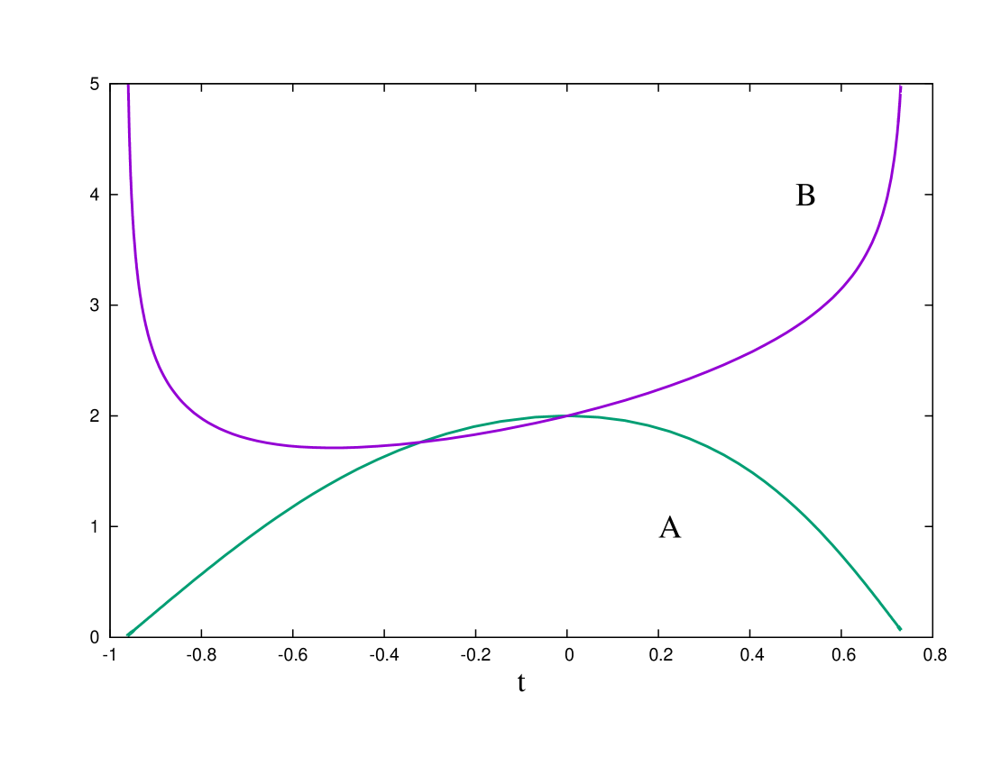
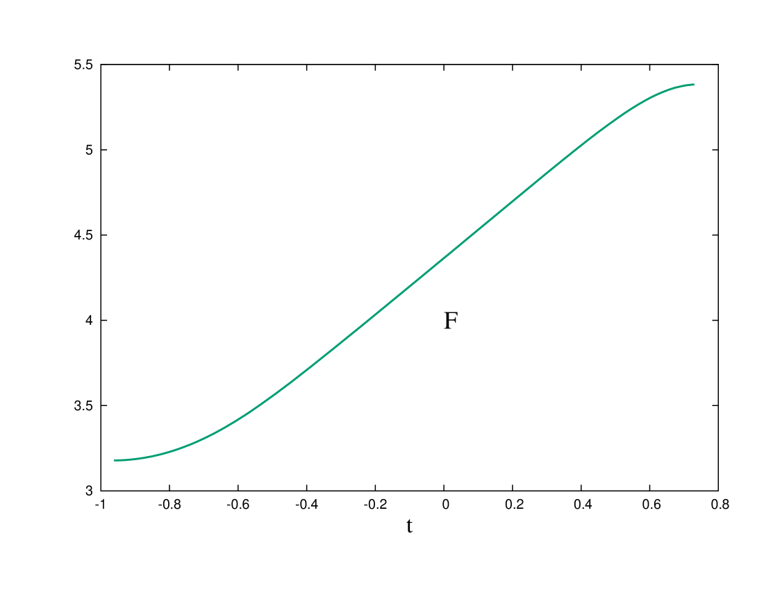
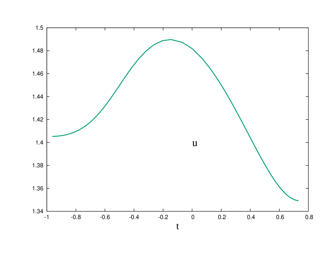
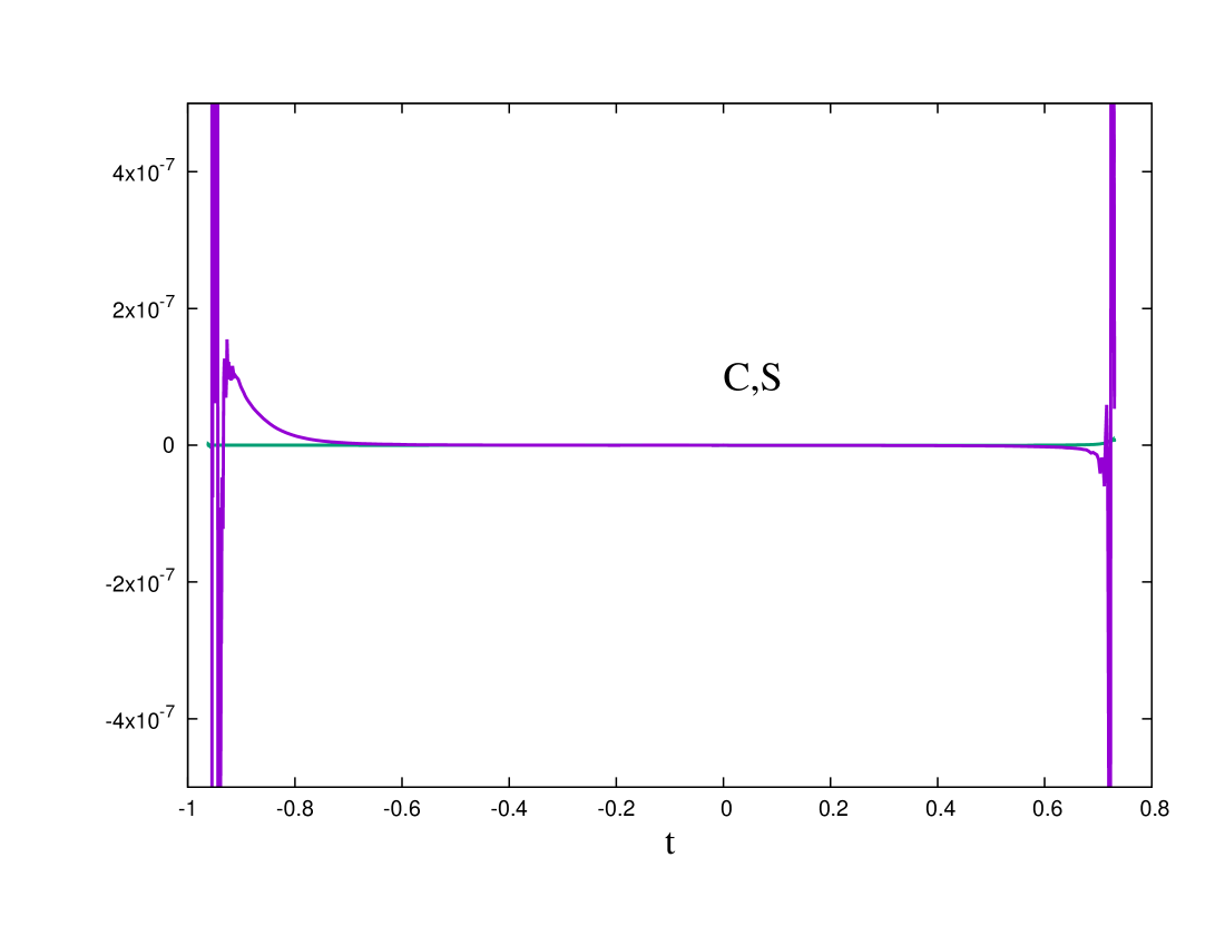
Figure 1: Evolution of initial data (8.2)–(8.4): singularity formation.

8.1 Generic initial values

Let us choose some values for the theory parameters, for example

$$b_{0}=1,\leavevmode\nobreak\ \leavevmode\nobreak\ \leavevmode\nobreak\ b_{1}=1,\leavevmode\nobreak\ \leavevmode\nobreak\ \leavevmode\nobreak\ b_{2}=2,\leavevmode\nobreak\ \leavevmode\nobreak\ \leavevmode\nobreak\ b_{3}=-5.$$ (8.1)

We choose next some arbitrary initial values for which the universe is anisotropic already at the initial time moment $t=0$. One should emphasise that the “initial moment” has nothing to do with the initial singularity but simply labels the timelike hypersurface containing the Cauchy data. For example, we chose

$$A_{0}=B_{0}=2,\leavevmode\nobreak\ \leavevmode\nobreak\ \leavevmode\nobreak\ \leavevmode\nobreak\ \leavevmode\nobreak\ \dot{A}_{0}=0,\leavevmode\nobreak\ \leavevmode\nobreak\ \leavevmode\nobreak\ \leavevmode\nobreak\ \dot{B}_{0}=1.$$ (8.2)

The equation ${\cal S}(u_{0})=0$ then shows two real roots, one of which is

$$u_{0}=1.4817.$$ (8.3)

Using this, the equation ${\cal C}(F_{0})=0$ gives

$$F_{0}=4.3649.$$ (8.4)

Integrating the equations with these initial conditions starting from $t=0$ towards $t>0$ and then towards $t<0$ gives the result shown in Fig 1.

The numerical solution extends over a finite interval. Close to its ends the $A$ amplitude becomes small and visibly approaches zero while the derivative $\dot{B}$ grows. This suggests that at the ends of the interval $A$ vanishes and the solution develops a curvature singularity which is difficult to approach numerically. At the same time, nothing visibly special happens to the $F$ and $u$ amplitudes. The constraints ${\cal C}$ and ${\cal S}$ both remain of the order of $10^{-9}$ and start to grow only close to the ends of the interval. Changing values of $b_{k}$ and $A_{0},B_{0},\dot{A}_{0},\dot{B}_{0}$ we find that this type of behaviour is typical – generic solutions develop singularities where one of the metric amplitudes vanishes and/or derivatives of other fields amplitudes grow. To avoid such a singular behaviour, we fine-tune the initial values.

8.2 Slightly perturbed type I FLRW

Let us see what happens if the initial values are close to type I FLRW solution. Choosing again the parameters $b_{k}$ according to (8.1), the equation $P_{1}(u_{\ast})=0$ has two roots:

$$u_{\ast} = -\frac{1}{5},\leavevmode\nobreak\ \leavevmode\nobreak\ \leavevmode\nobreak\ \leavevmode\nobreak\ \leavevmode\nobreak\ \leavevmode\nobreak\ \leavevmode\nobreak\ P_{0}(u_{\ast})=0.68,\leavevmode\nobreak\ \leavevmode\nobreak\ \leavevmode\nobreak\ \leavevmode\nobreak\ \leavevmode\nobreak\ \leavevmode\nobreak\ \leavevmode\nobreak\ H(u_{\ast})=\sqrt{P_{0}(u_{\ast})/3}={0.476};$$

$$u_{\ast} = 1,\leavevmode\nobreak\ \leavevmode\nobreak\ \leavevmode\nobreak\ \leavevmode\nobreak\ \leavevmode\nobreak\ \leavevmode\nobreak\ \leavevmode\nobreak\ \leavevmode\nobreak\ \leavevmode\nobreak\ \leavevmode\nobreak\ P_{0}(u_{\ast})=5,\leavevmode\nobreak\ \leavevmode\nobreak\ \leavevmode\nobreak\ \leavevmode\nobreak\ \leavevmode\nobreak\ \leavevmode\nobreak\ \leavevmode\nobreak\ \leavevmode\nobreak\ \leavevmode\nobreak\ \leavevmode\nobreak\ \leavevmode\nobreak\ H(u_{\ast})=\sqrt{P_{0}(u_{\ast})/3}=1.29.$$ (8.5)

Since for each of these roots one has $P_{0}(u_{\ast})>0$ (which is not the case for arbitrary values of $b_{k}$), the cosmological constant $P_{0}(u_{\ast})/3$ is positive, hence each root gives rise to a type I FLRW solution with its own Hubble rate $H(u_{\ast})$.

Let us select the first root in (8.2), $u_{\ast}=-1/5$, and then choose the initial values of $A,B,\dot{A},\dot{B}$ to be “almost” type I FLRW (we set here ${\bf a}=10$),

$$A_{0}=B_{0}={\bf a},\leavevmode\nobreak\ \leavevmode\nobreak\ \leavevmode\nobreak\ \leavevmode\nobreak\ \leavevmode\nobreak\ \dot{A}_{0}=\sqrt{1+H^{2}(u_{\ast}){\bf a}^{2}},\leavevmode\nobreak\ \leavevmode\nobreak\ \leavevmode\nobreak\ \leavevmode\nobreak\ \dot{B}_{0}=\dot{A}+\delta.$$ (8.6)

For $\delta=0$ these values are precisely type I FLRW. To make them “slightly anisotropic” we choose $\delta=-0.1$. Then the initial value $u_{0}$ is no longer exactly $u_{\ast}=-0.2$ but is determined by the ${\cal S}(u_{0})=0$ constraint, which has four real roots,

$$u_{0}^{(1)}=-0.231122,\leavevmode\nobreak\ \leavevmode\nobreak\ \leavevmode\nobreak\ \leavevmode\nobreak\ u_{0}^{(2)}=-0.233943,\leavevmode\nobreak\ \leavevmode\nobreak\ \leavevmode\nobreak\ \leavevmode\nobreak\ u_{0}^{(3)}=-0.152569,\leavevmode\nobreak\ \leavevmode\nobreak\ \leavevmode\nobreak\ \leavevmode\nobreak\ u_{0}^{(4)}=-0.645204.$$ (8.7)

The ${\cal C}(F_{0})=0$ constraint then gives, correspondingly, the values

$$F_{0}^{(1)}=-0.831254,\leavevmode\nobreak\ \leavevmode\nobreak\ \leavevmode\nobreak\ \leavevmode\nobreak\ F_{0}^{(2)}=-0.905497,\leavevmode\nobreak\ \leavevmode\nobreak\ \leavevmode\nobreak\ \leavevmode\nobreak\ F_{0}^{(3)}=-2.95427,\leavevmode\nobreak\ \leavevmode\nobreak\ \leavevmode\nobreak\ \leavevmode\nobreak\ F_{0}^{(4)}=-0.323448.$$ (8.8)

       

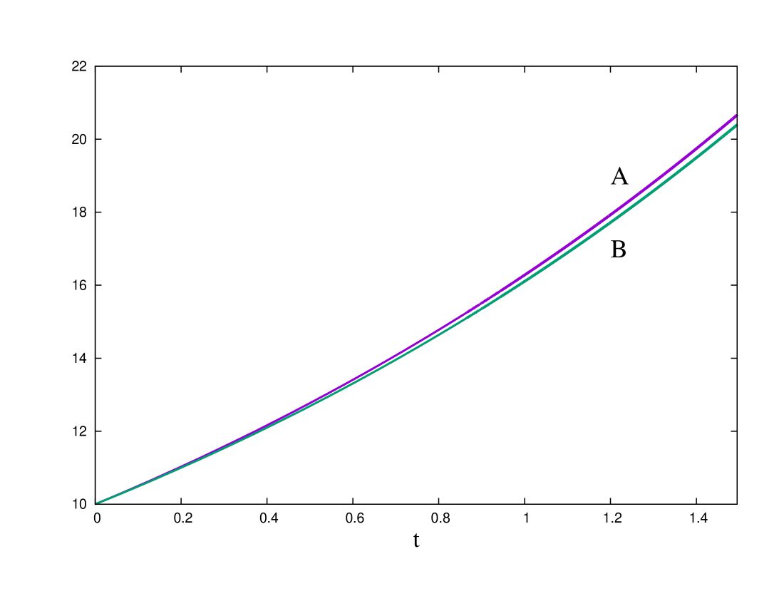
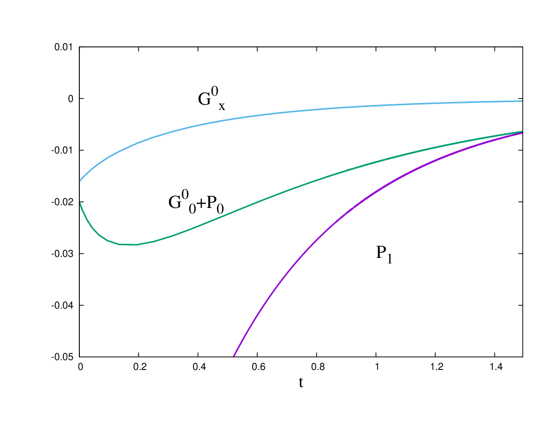
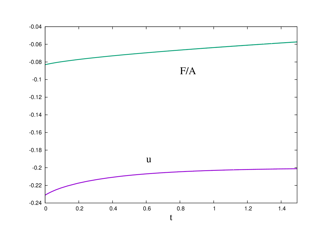
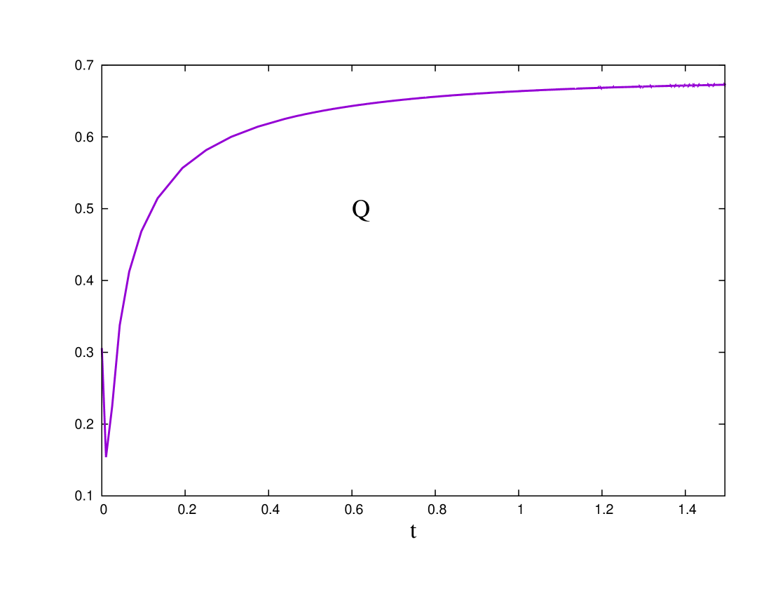
Figure 2: Evolution of a weakly perturbed type I solution – relaxation to type II FLRW.

We see that the values $u_{0}^{(1)}$ and $u_{0}^{(2)}$ are closer to $u_{\ast}=-0.2$ than $u_{0}^{(3)}$ and $u_{0}^{(4)}$. Therefore, although the g-metric is almost isotropic, the Stueckelberg fields in the latter two cases are far from type I FLRW value, hence such initial values actually corresponds to a strong perturbation. This is confirmed by the numerics – solutions generated by the initial choice $u_{0}=u_{0}^{(3)}$ or $u_{0}=u_{0}^{(4)}$ develop a curvature singularity similar to that discussed in the previous subsection.

Let us now see what happens if $u_{0}=u_{0}^{(1)}$ or $u_{0}=u_{0}^{(2)}$ so that the initial values are closer to type I FLRW configuration. It turns out that solutions obtained in these two cases are almost identical and we therefore describe only the $u_{0}=u_{0}^{(1)}$ solution shown in Fig.2.

As one can see in Fig.2, the $A$ and $B$ amplitudes always stay very close to each other, while the whole configuration becomes “more and more isotropic”. Indeed, both for type I and type II FLRW isotropic solutions one has $P_{1}=G^{0}_{x}=G^{0}_{0}+P_{0}=0$ and $u=u_{\ast}$. At the same time, one sees in Fig.2 that $P_{1}$, $G^{0}_{x}$ and $G^{0}_{0}+P_{0}$ approach zero while $u$ approaches $u_{\ast}$. Therefore, the solution approaches either type I or type II FLRW. Now, if it was type I FLRW then the ratio $F/A$ would approach $u_{\ast}$, which is clearly not the case as is seen in Fig.2. Therefore, the solution must approach type II FLRW. To verify this we plot in Fig.2 the function

$$Q=\sqrt{\frac{F\dot{F}}{u_{\ast}^{2}A}}.$$ (8.9)

For type II FLRW solutions (5.25) this functions assumes a constant value $Q(t)=q$, which is the integration constant in (5.25). For our solution, as is seen in Fig.2, $Q(t)$ approaches a constant value, hence the solution indeed approaches the isotropic type II FLRW background (5.25) with $q=Q(\infty)$.

We find a similar behaviour also for all other choices of the theory parameters $b_{k}$ that we considered. It is difficult to extend numerical solutions to large values of $A,B$ since the constraints start to grow, but using the multi-shooting method we managed to keep them under control and extend the solutions to the region where $P_{1}$, $G^{0}_{x}$ and $G^{0}_{0}+P_{0}$ become very small while $Q(t)$ become almost constant. Since such solutions seem to exist for generic parameter values, we conclude that slightly perturbed type I configurations evolve towards type II FLRW isotropic fixed point (5.25).

       

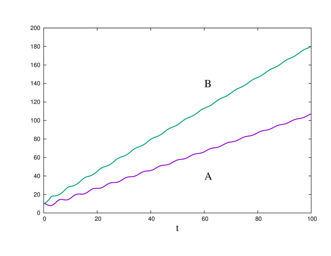
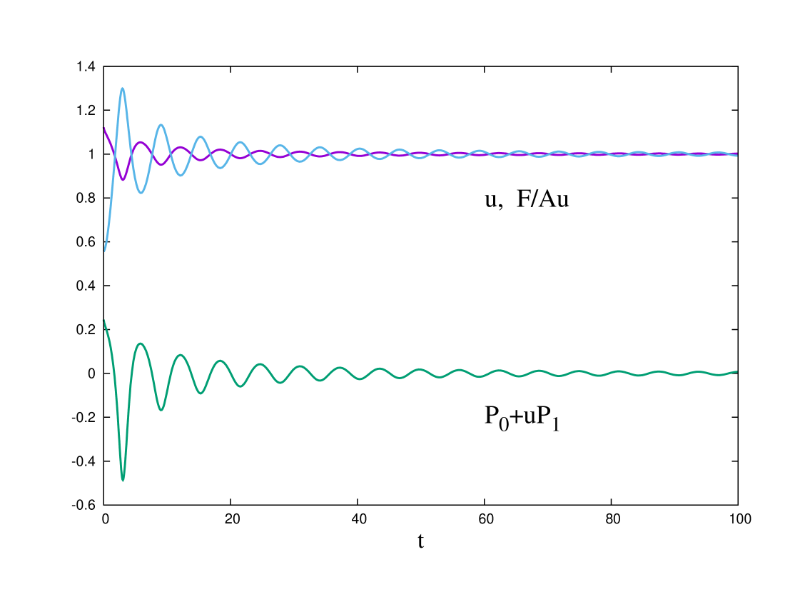
Figure 3: Evolution of strongly perturbed type I FLRW – decay into flat space.

8.3 Strongly perturbed type I FLRW – decay into flat space

We have already mentioned above what is meant by strong perturbations – parameterising the initial values similarly to (8.6) and choosing the root of ${\cal S}(u_{0})=0$ to be far from the root of $P_{1}(u_{\ast})=0$. As a result, the physical geometry is initially close to that for type I FLRW solution but the Stueckelberg fields are different. As was mentioned above, the evolution of such initial data generically leads to a curvature singularity. However, we were able to find parameter values for which the outcome is different. Specifically, choosing

$$b_{0}=-19,\leavevmode\nobreak\ \leavevmode\nobreak\ \leavevmode\nobreak\ \leavevmode\nobreak\ b_{1}=14,\leavevmode\nobreak\ \leavevmode\nobreak\ \leavevmode\nobreak\ \leavevmode\nobreak\ b_{2}=-10,\leavevmode\nobreak\ \leavevmode\nobreak\ \leavevmode\nobreak\ \leavevmode\nobreak\ b_{3}=7,$$ (8.10)

one root of $P_{1}(u_{\ast})=0$ is $u_{\ast}=1.63$ with $H(u_{\ast})=\sqrt{P_{0}(u_{\ast})/3}=0.15$. Using this to compute $A_{0},B_{0},\dot{A}_{0},\dot{B}_{0}$ in (8.6) (with ${\bf a}=10$ and $\delta=-0.1$) and then solving the ${\cal S}(u_{0})=0$ constraint gives four real roots,

$$u_{0}^{(1)}=1.1222,\leavevmode\nobreak\ \leavevmode\nobreak\ \leavevmode\nobreak\ \leavevmode\nobreak\ \leavevmode\nobreak\ u_{0}^{(2)}=1.5909,\leavevmode\nobreak\ \leavevmode\nobreak\ \leavevmode\nobreak\ \leavevmode\nobreak\ \leavevmode\nobreak\ u_{0}^{(3)}=1.6362,\leavevmode\nobreak\ \leavevmode\nobreak\ \leavevmode\nobreak\ \leavevmode\nobreak\ \leavevmode\nobreak\ u_{0}^{(4)}=1.6680.$$ (8.11)

The root $u_{0}^{(3)}=1.6362$ is the closest to $u_{\ast}=1.63$ and gives rise to a slightly perturbed type I configuration that relaxes to type II FLRW. Let us consider instead $u_{0}^{(1)}=1.1222$ – the farthest from $u_{\ast}=1.63$ root. Surprisingly, the evolution of this initial data does not lead to a singularity but to something different – a decay into flat spacetime. As shown in Fig.3, the fields show damped oscillations and at late times the $A$ and $B$ amplitudes become linear functions of time, $u$ approaches a constant value such that the combination $P_{0}+uP_{1}$ tends to zero, while ${\cal A}=F/Au$ tends to one. Therefore, the fields approach the flat spacetime solution described by Eqs.(A.7)–(A.11) in Appendix A:

$$A={\bf a}=t,\leavevmode\nobreak\ \leavevmode\nobreak\ \leavevmode\nobreak\ \leavevmode\nobreak\ \leavevmode\nobreak\ B=Ae^{\chi},\leavevmode\nobreak\ \leavevmode\nobreak\ \leavevmode\nobreak\ \leavevmode\nobreak\ F={\cal A}{\bf a}u,\leavevmode\nobreak\ \leavevmode\nobreak\ \leavevmode\nobreak\ \leavevmode\nobreak\ {\cal A}=1,\leavevmode\nobreak\ \leavevmode\nobreak\ \leavevmode\nobreak\ \leavevmode\nobreak\ \leavevmode\nobreak\ P_{0}(u)+uP_{1}(u)=0.$$ (8.12)

It should be emphasised that we did not find such solutions for generic $b_{k}$.

9 Conclusions

To recapitulate, we studied above the fully non-linear dynamics of anisotropic deformations of the homogeneous and isotropic cosmology in the ghost free massive gravity with flat reference metric. We found that when perturbed, this solution cannot relax to itself in the long run, hence it is unstable. If the initial perturbation is not too strong, it relaxes instead to type II FLRW solution whose physical metric is also de Sitter. Therefore, the geometry described by the physical g-metric is stable and does relax to itself. However, during the relaxation and damping of the anisotropies the Stueckelberg scalars change in such a way that the f-metric evolves from type I to type II FLRW value and looses some of the isometries that were common for both metrics.

The final type II FLRW configuration seems to be an attractor within the considered class of anisotropic metrics. This is confirmed by the analysis of linear modes in its vicinity and also by the numerics which show that slightly perturbed type I FLRW configurations evolve towards type II FLRW solutions. It is natural to wonder if the latter is itself stable with respect to more general deformations. We leave this issue as well as the problem of detecting possible ghosts to a separate study.

If the initial perturbation is strong, then the initially isotropic solution completely changes its structure. In the generic case it ends up in a singular state, but for some parameter values it can also decay into flat space. To pin down the parameter regions where the latter possibility is realised requires a separate study.

Appendix A Isotropic solutions with either $\dot{f}=0$ or $F=0$

We describe in this Appendix the remaining solutions of equations (5),(5). Specifically, to solve the second equation in (5),

$$\frac{F^{2}}{Y}\,\dot{f}P_{1}=0,$$ (A.1)

it was assumed in Section 5 that $P_{1}=0$. Let us now consider the other two options and assume first that $\dot{f}=0.$ Then (4.8) implies that $Y=\dot{F}+{F}/{{\bf a}},$ in which case equations (5) and the first equation in (5) reduce to

$$E_{0} \equiv \frac{3\dot{{\bf a}}^{2}}{{\bf a}^{2}}-\frac{3}{{\bf a}^{2}}=P_{0}+\frac{F}{{\bf a}}P_{1},$$ (A.2)

$$E_{1} \equiv \frac{\ddot{{\bf a}}}{{\bf a}}+\frac{2\dot{{\bf a}}^{2}}{{\bf a}^{2}}-\frac{2}{{\bf a}^{2}}=P_{0}+\frac{1}{2}\,\left(\dot{F}+\frac{F}{{\bf a}}\right)P_{1}\,,$$ (A.3)

$$0 = \left(u-\frac{F}{{\bf a}}\right)\left(P_{1}+\frac{1}{2}(\dot{F}-u)dP_{1}\right).$$ (A.4)

Due to the Bianchi identity,

$$\dot{E}_{0}=6\,\frac{\dot{a}}{a}\,(E_{1}-E_{0}),$$ (A.5)

equation (A.3) can be replaced by

$$\left(P_{0}+\frac{F}{{\bf a}}\,P_{1}\right)^{\mbox{.}}=3\,\frac{\dot{{\bf a}}}{{\bf a}}\,\left(\dot{F}-\frac{F}{{\bf a}}\right)P_{1}\,.$$ (A.6)

Next, (4.16) and (5.2) imply

$$F=e^{\chi-f}{\bf a}u\equiv{\cal A}{\bf a}u\,,$$ (A.7)

with constant ${\cal A}$. Inserting this to (A.2),(A.4),(A.6) one obtains

$$\left(P_{0}+{\cal A}uP_{1}\right)^{\mbox{.}} = 3{\cal A}\,\frac{\dot{{\bf a}}}{{\bf a}}\,\left(({\bf a}u)^{\mbox{.}}-u\right)P_{1},$$ (A.8)

$$(1-{\cal A}) u \left(2P_{1}+[{\cal A}({\bf a}u)^{\mbox{.}}-u]dP_{1}\right)=0,$$ (A.9)

$$\frac{3}{{\bf a}^{2}}(\dot{{\bf a}}^{2}-1) = P_{0}+{\cal A}uP_{1}.$$ (A.10)

Equation (A.9) contains the product of three factors.

Let us assume that ${\cal A}=1$, hence the first factor in (A.9) vanishes and the equation is fulfilled. Using $\dot{P}_{m}=dP_{m}\,\dot{u}$ and the relation (4.19), equation (A.8) then reduces to

$$\dot{u}=\frac{\dot{{\bf a}}}{{\bf a}}\,\left(({\bf a}u)^{\mbox{.}}-u\right),$$

which is equivalent to

$$({\bf a}u)^{\mbox{.}}(\dot{{\bf a}}-1)=0.$$ (A.11)

One solution of this is $\dot{{\bf a}}=1$ hence ${\bf a}=t$, which corresponds to flat (Milne) space, while (A.10) then gives the condition on $u$,

$$0=P_{0}(u)+uP_{1}(u).$$ (A.12)

Other possibility to fulfill (A.11) is to set ${\bf a}u=F_{0}=const.$ hence $u=F_{0}/{\bf a}$. Equation (A.10) then reduces to

$$\frac{3}{{\bf a}^{2}}(\dot{{\bf a}}^{2}-1)=P_{0}+uP_{1}=b_{0}+\frac{3b_{1}F_{0}}{{\bf a}}+\frac{3b_{2}F_{0}^{2}}{{\bf a}^{3}}+\frac{b_{3}F_{0}^{3}}{{\bf a}^{3}}.$$ (A.13)

The four terms on the right here can be viewed as contributions of the graviton interaction terms that mimic a cosmological term, a gas of domain walls, a gas of cosmic strings, and a dust, respectively. This solution is actually known [5], [8]. However, since $F=F_{0}$, the reference metric (4.2) is degenerate.

Let us now consider the case where ${\cal A}\neq 1$ and assume first that $\dot{u}\neq 0$. Then (A.9) requires that $2P_{1}+[{\cal A}({\bf a}u)^{\mbox{.}}-u]dP_{1}=0.$ After simple transformations one can show that this condition, together with (A.8), are equivalent to the following two conditions:

$$-\frac{\dot{{\bf a}}}{{\bf a}}+\frac{1}{{\bf a}}+\frac{(c-1)\dot{P}_{1}}{3P_{1}}=0,\leavevmode\nobreak\ \leavevmode\nobreak\ \leavevmode\nobreak\ \leavevmode\nobreak\ \leavevmode\nobreak\ \leavevmode\nobreak\ \leavevmode\nobreak\ \leavevmode\nobreak\ \leavevmode\nobreak\ \leavevmode\nobreak\ \leavevmode\nobreak\ \frac{\dot{{\bf a}}}{{\bf a}}+\frac{\dot{u}}{u}+\frac{dP_{0}}{{\cal A}{\bf a}u\,dP_{1}}=0.$$ (A.14)

These conditions can be resolved to algebraically express ${\bf a}$ and $\dot{{\bf a}}$ in terms of $u$ and $\dot{u}$,

$${\bf a}={\bf a}(u,\dot{u}),\leavevmode\nobreak\ \leavevmode\nobreak\ \leavevmode\nobreak\ \leavevmode\nobreak\ \leavevmode\nobreak\ \leavevmode\nobreak\ \leavevmode\nobreak\ \dot{{\bf a}}=\dot{{\bf a}}(u,\dot{u}).$$ (A.15)

Injecting this to (A.10) gives a first order differential equation for $u$,

$$\dot{u}^{2}={\cal Q}(u),$$ (A.16)

with a complicated function ${\cal Q}(u)$. In addition, (A.15) implies that

$$\frac{\partial{\bf a}(u,\dot{u})}{\partial u}\,\dot{u}+\frac{\partial{\bf a}(u,\dot{u})}{\partial\dot{u}}\,\ddot{u}=\dot{{\bf a}}(u,\dot{u}),$$ (A.17)

which yields a second order differential equation for $u$. Therefore, if $u$ is not constant, it should fulfill two differential equations (A.16) and (A.17). However, (A.16) implies in this case that

$$\dot{u}=\pm\sqrt{{\cal Q}(u)},\leavevmode\nobreak\ \leavevmode\nobreak\ \leavevmode\nobreak\ \leavevmode\nobreak\ \leavevmode\nobreak\ \ddot{u}=\frac{1}{2}\frac{\partial{\cal Q}(u)}{\partial u},$$

injecting which to (A.17) gives a non-trivial algebraic condition on $u$. It follows therefore that $u$ should be constant, hence the assumption $\dot{u}\neq 0$ leads to a contradiction.

Let us therefore return to Eqs.(A.14) and set $\dot{u}=0$. This gives

$$\dot{a}=1,\leavevmode\nobreak\ \leavevmode\nobreak\ \leavevmode\nobreak\ \leavevmode\nobreak\ \leavevmode\nobreak\ \leavevmode\nobreak\ {\cal A}=-\frac{dP_{0}(u)}{u\,dP_{1}(u)},$$ (A.18)

injecting which to (A.10) leads to

$$P_{0}(u)\,dP_{1}(u)-P_{1}(u)\,dP_{0}(u)=0.$$ (A.19)

These conditions determine values of $u$ and ${\cal A}$, whereas the spacetime metric is again flat.

We note finally that one more possibility to solve Eq.(A.9) is to set $u=0$. Equations (A.8)–(A.10) then reduce to

$$\frac{3}{{\bf a}^{2}}(\dot{{\bf a}}^{2}-1)=P_{0}(u),$$ (A.20)

however, since $F={\cal A}{\bf a}u=0$, the reference metric is again degenerate. Yet one more solution of this type can be obtained by returning to (A.1) and setting there $F=0$. It follows then from (4.8) that $Y=0$ and $F^{2}/Y=0$ hence equations (A.2)–(A.4) reduce again to (A.20) with $u$ defined by

$$u\,dP_{0}(u)=2u(b_{1}+b_{2}\,u)=0.$$ (A.21)

Hence setting $u=-b_{1}/b_{2}$ in (A.20) gives one more solution with $F=0$. The reference metric is again degenerate.

Summarising, solutions of (A.8)–(A.10) split into two classes. First, there are solutions describing a flat Milne spacetime,

$$ds_{g}^{2}=-dt^{2}+t^{2}\left(dx^{2}+e^{2x}[dy^{2}+dz^{2}]\right),$$

$$ds_{f}^{2}=-({\cal A}u)^{2}dt^{2}+t^{2}\left(({\cal A}u)^{2}dx^{2}+e^{2x}[dy^{2}+dz^{2}]\right).$$ (A.22)

Here one has either ${\cal A}=1$ while $u$ fulfills the cubic equation (A.12) which can have up to three real roots, or ${\cal A}$ is determined by (A.18) while $u$ fulfills the cubic equation (A.19) which can also have up to three real roots. Therefore, there can be up to six different values of ${\cal A}u$ and hence six different flat space solutions. These solutions may have different properties.

Other solutions of (A.8)–(A.10) are of the FLRW type with the scale factor determined either by (A.13) or by (A.20), (A.21). However, one has in this case $F=const.$ hence $dF=0$ so that the reference metric is degenerate.

Appendix B Stueckelberg scalars and new type II FLRW solutions

It turns out that type II FLRW isotropic solution (5.2) can be promoted to an infinite dimensional family of new solutions. To see this let us first check how this solution looks when expressed in the form similar to (3.8), (3.10). Making the coordinate shift $x\to x-\chi$ Eq.(5.2) becomes

$$ds_{g}^{2} = -dt^{2}+{\bf a}^{2}dx^{2}+e^{2x}\left[{\bf a}^{2}\left[dy^{2}+dz^{2}\right]\right],$$

$$ds_{f}^{2} = -dF^{2}+F^{2}\left(dX^{2}+e^{2X}[dy^{2}+dz^{2}]\right),\leavevmode\nobreak\ \leavevmode\nobreak\ \leavevmode\nobreak\ \leavevmode\nobreak\ \leavevmode\nobreak\ \leavevmode\nobreak\ \leavevmode\nobreak\ \leavevmode\nobreak\ X=x+f(t)-\chi.$$ (B.1)

Combining formulas (3.5), (5.23), (5.24) one can relate the $t,x,y,z$ coordinates to coordinates of 5D Minkowski space used in (3.8),

$$x^{0} = \frac{{\bf a}}{2}\left(e^{-x}+e^{x}(y^{2}+z^{2}+1)\right),\leavevmode\nobreak\ \leavevmode\nobreak\ \leavevmode\nobreak\ x^{1}={\bf a}\,e^{x}y,\leavevmode\nobreak\ \leavevmode\nobreak\ \leavevmode\nobreak\ \leavevmode\nobreak\ \leavevmode\nobreak\ x^{2}={\bf a}\,e^{x}z,\leavevmode\nobreak\ \leavevmode\nobreak\ \leavevmode\nobreak\$$

$$x^{3} = \frac{{\bf a}}{2}\left(e^{-x}+e^{x}(y^{2}+z^{2}-1)\right).$$ (B.2)

The inverse transformation is

$${\bf a}\,e^{x}=x^{0}-x^{3},\leavevmode\nobreak\ \leavevmode\nobreak\ \leavevmode\nobreak\ \leavevmode\nobreak\ \leavevmode\nobreak\ \leavevmode\nobreak\ y=\frac{x^{1}}{x^{0}-x^{3}},\leavevmode\nobreak\ \leavevmode\nobreak\ \leavevmode\nobreak\ \leavevmode\nobreak\ \leavevmode\nobreak\ \leavevmode\nobreak\ z=\frac{x^{2}}{x^{0}-x^{3}},$$

$${\bf a}^{2}=(x^{0})^{2}-(x^{1})^{2}-(x^{2})^{2}-(x^{3})^{2}=(x^{4})^{2}-\frac{1}{H^{2}}.$$ (B.3)

These relations bring the de Sitter g-metric expressed in the form (B) to the form (3.8) and back. Similarly, the f-metric in (B) is transformed to the form (3.10) with

$$X^{0} = \frac{F}{2}\left(e^{-X}+e^{X}(y^{2}+z^{2}+1)\right),\leavevmode\nobreak\ \leavevmode\nobreak\ \leavevmode\nobreak\ X^{1}=F\,e^{X}y,\leavevmode\nobreak\ \leavevmode\nobreak\ \leavevmode\nobreak\ \leavevmode\nobreak\ \leavevmode\nobreak\ X^{2}=F\,e^{X}z,\leavevmode\nobreak\ \leavevmode\nobreak\ \leavevmode\nobreak\$$

$$X^{3} = \frac{F}{2}\left(e^{-X}+e^{X}(y^{2}+z^{2}-1)\right).$$ (B.4)

There remains to express these in terms of $x^{0}$, …, $x^{4}$. One has from (5.25) $e^{f-\chi}=u_{\ast}\,{\bf a}/F$ while $F=u_{\ast}\,\sqrt{w}{\bf a}$, hence $Fe^{X}=u_{\ast}\,{\bf a}\,e^{x}$ and $Fe^{-X}=u_{\ast}\,{\bf a}\,w\,e^{-x}$. Using this and (B) together with (5.18) yields the Stueckelberg fields $X^{A}$ expressed in terms of the 5D Minkowski coordinates,

$$X^{0}=u_{\ast}\,\left(x^{0}+\frac{1}{2}\,D\right),\leavevmode\nobreak\ \leavevmode\nobreak\ \leavevmode\nobreak\ \leavevmode\nobreak\ X^{1}=u_{\ast}\,x^{1},\leavevmode\nobreak\ \leavevmode\nobreak\ \leavevmode\nobreak\ \leavevmode\nobreak\ X^{2}=u_{\ast}\,x^{2},\leavevmode\nobreak\ \leavevmode\nobreak\ \leavevmode\nobreak\ \leavevmode\nobreak\ X^{3}=u_{\ast}\,\left(x^{3}+\frac{1}{2}\,D\right),$$ (B.5)

where

$$D=\frac{(w-1)\,{\bf a}^{2}}{(x^{0}-x^{3})}=\frac{(Hx^{4}-q^{2})^{2}}{H^{2}(x^{3}-x^{0})}.$$ (B.6)

Let us introduce lightlike coordinates $U=x^{3}-x^{0}$ and $V=x^{3}+x^{0}$. Then the two metrics in (B) can be represented as

$$ds_{g}^{2} = dUdV+(x^{1})^{2}+(x^{2})^{2}+(x^{4})^{2}\,,$$

$$\frac{1}{u_{\ast}^{2}}\,ds_{f}^{2} = dUd(V+D)+(x^{1})^{2}+(x^{2})^{2}+(x^{4})^{2}\,,$$ (B.7)

where

$$UV+(x^{1})^{2}+(x^{2})^{2}+(x^{4})^{2}=\frac{1}{H^{2}},$$ (B.8)

and

$$D=\frac{(Hx^{4}-q^{2})^{2}}{H^{2}U}.$$ (B.9)

This can be generalised to an infinite dimensional family of new solutions. Specifically, it is known [31] (see also [10]) that if $P_{1}=0$ and $g_{\mu\nu}$ fulfills the Einstein equations with the cosmological constant $P_{0}$ while the two metrics fulfill the Gordon relation,

$$f_{\mu\nu}=\omega^{2}\left[g_{\mu\nu}+(1-\zeta^{2}){\rm V}_{\mu}{\rm V}_{\nu}\right],$$ (B.10)

where $\omega,\zeta$ are some functions and ${\rm V}_{\mu}$ is a unit timelike vector,

$$g^{\mu\nu}{\rm V}_{\mu}{\rm V}_{\nu}=-1,$$ (B.11)

then the dRGT field equations are satisfied. Now, the g-metric in (B.7) is de Sitter with the Hubble parameter $H^{2}=P_{0}(u_{\ast})/3$ where $P_{1}(u_{\ast})=0$. Moreover, the two metrics in (B.7) are related to each other via

$$ds_{g}^{2}=u_{\ast}^{2}\left[ds_{g}^{2}+dUdD-(dx^{4})^{2}\right],$$ (B.12)

hence the Gordon relation will be fulfilled if

$$\partial_{(\mu}U\partial_{\nu)}D-\partial_{\mu}x^{4}\partial_{\nu}x^{4}=(1-\zeta^{2}){\rm V}_{\mu}{\rm V}_{\nu}\,.$$ (B.13)

Let us assume that $D=D(U,x^{4})$ and that the vector ${\rm V}_{\mu}$ has non-vanishing components only along the $U$ and $x^{4}$ directions. Then (B.13) reduce to

$$\partial_{U}D = (1-\zeta^{2}){\rm V}_{U}^{2}\,,$$

$$\frac{1}{2}\,\partial_{4}D = (1-\zeta^{2}){\rm V}_{U}{\rm V}_{4}\,,$$

$$-1 = (1-\zeta^{2}){\rm V}_{4}^{2}\,.$$ (B.14)

Taking the square of the second relation and using the two others gives

$$\frac{1}{4}\,\left(\partial_{4}D\right)^{2}=(1-\zeta^{2}){\rm V}^{2}_{U}(1-\zeta^{2}){\rm V}_{4}^{2}=-(1-\zeta^{2}){\rm V}^{2}_{U}=-\partial_{U}D,$$ (B.15)

hence

$$\partial_{U}D+\frac{1}{4}\,\left(\partial_{4}D\right)^{2}=0.$$ (B.16)

Any solution of this PDE provides a cosmological solution of the dRGT theory written in the form (B.7),(B.8). This gives an infinite dimensional family of new homogeneous and isotropic type II FLRW cosmologies.

References

- [1] A. Riess et al., Observational evidence from supernovae for an accelerating universe and a cosmological constant, Astron.Journ. 116 (1998) 1009.
- [2] S. Perlmutter et al., Measurements of and from 42 high-redshift supernovae, Astrophys.Journ. 517 (1999) 565.
- [3] C. de Rham, G. Gabadadze and A. Tolley, Resummation of massive gravity, Phys.Rev.Lett. 106 (2011) 231101, [1011.1232].
- [4] A. Gumrukcuoglu, C. Lin and S. Mukohyama, Open FRW universes and self-acceleration from nonlinear massive gravity, JCAP 1111 (2011) 030, [1109.3845].
- [5] A. Chamseddine and M. Volkov, Cosmological solutions with massive gravitons, Phys.Lett. B704 (2011) 652–654, [1107.5504].
- [6] G. D’Amico, C. de Rham, S. Dubovsky, G. Gabadadze, D. Pirtskhalava et al., Massive cosmologies, Phys.Rev. D84 (2011) 124046, [1108.5231].
- [7] M. Volkov, Exact self-accelerating cosmologies in the ghost-free bigravity and massive gravity, Phys.Rev. D86 (2012) 061502, [1205.5713].
- [8] M. Volkov, Exact self-accelerating cosmologies in the ghost-free massive gravity – the detailed derivation, Phys.Rev. D86 (2012) 104022, [1207.3723].
- [9] T. Kobayashi, M. Siino, M. Yamaguchi and D. Yoshida, New cosmological solutions in massive gravity, Phys.Rev. D86 (2012) 061505, [1205.4938].
- [10] C. Mazuet and M. Volkov, De Sitter vacua in ghost-free massive gravity theory, Phys. Lett. B751 (2015) 19–24, [1503.03042].
- [11] E. Gumrukcuoglu, C. Lin and S. Mukohyama, Cosmological perturbations of self-accelerating universe in nonlinear massive gravity, JCAP 1203 (2012) 006, [1111.4107].
- [12] A. De Felice, E. Gumrukcuoglu and S. Mukohyama, Massive gravity: nonlinear instability of the homogeneous and isotropic universe, Phys.Rev.Lett. 109 (2012) 171101, [1206.2080].
- [13] A. De Felice, A. E. Gumrukcuoglu, C. Lin and S. Mukohyama, Nonlinear stability of cosmological solutions in massive gravity, JCAP 1305 (2013) 035, [1303.4154].
- [14] S. Hassan and R. A. Rosen, Bimetric gravity from ghost-free massive gravity, JHEP 1202 (2012) 126, [1109.3515].
- [15] M. Volkov, Cosmological solutions with massive gravitons in the bigravity theory, JHEP 1201 (2012) 035, [1110.6153].
- [16] Y. Akrami, S. F. Hassan, F. K?nnig, A. Schmidt-May and A. R. Solomon, Bimetric gravity is cosmologically viable, Phys. Lett. B748 (2015) 37–44, [1503.07521].
- [17] A. De Felice and S. Mukohyama, Towards consistent extension of quasidilaton massive gravity, Phys. Lett. B728 (2014) 622–625, [1306.5502].
- [18] S. Mukohyama, A new quasidilaton theory of massive gravity, JCAP 1412 (2014) 011, [1410.1996].
- [19] A. De Felice, S. Mukohyama and M. Oliosi, Minimal quasidilaton, 1701.01581.
- [20] G. D’Amico, G. Gabadadze, L. Hui and D. Pirtskhalava, Quasidilaton: theory and cosmology, Phys. Rev. D87 (2013) 064037, [1206.4253].
- [21] G. Gabadadze, R. Kimura and D. Pirtskhalava, Self-acceleration with quasidilaton, Phys. Rev. D90 (2014) 024029, [1401.5403].
- [22] C. de Rham, M. Fasiello and A. J. Tolley, Stable FLRW solutions in generalized massive gravity, Int.J.Mod.Phys. D23 (2014) 3006, [1410.0960].
- [23] A. De Felice and S. Mukohyama, Minimal theory of massive gravity, Phys. Lett. B752 (2016) 302–305, [1506.01594].
- [24] A. De Felice and S. Mukohyama, Phenomenology in minimal theory of massive gravity, JCAP 1604 (2016) 028, [1512.04008].
- [25] A. De Felice and S. Mukohyama, Graviton mass reduces tension between early and late time cosmological data, 1607.03368.
- [26] E. Gumrukcuoglu, C. Lin and S. Mukohyama, Anisotropic Friedmann - Robertson - Walker universe from nonlinear massive gravity, Phys.Lett. B717 (2012) 295–298, [1206.2723].
- [27] T. Q. Do and W. F. Kao, Anisotropically expanding universe in massive gravity, Phys. Rev. D88 (2013) 063006.
- [28] K.-i. Maeda and M. Volkov, Anisotropic universes in the ghost-free bigravity, 1302.6198.
- [29] P. Motloch, W. Hu, A. Joyce and H. Motohashi, Self-accelerating massive gravity: superluminality, Cauchy surfaces and strong coupling, Phys. Rev. D92 (2015) 044024, [1505.03518].
- [30] P. Motloch, W. Hu and H. Motohashi, Self-accelerating massive gravity: hidden constraints and characteristics, Phys. Rev. D93 (2016) 104026, [1603.03423].
- [31] V. Baccetti, P. Martin-Moruno and M. Visser, Gordon and Kerr-Schild ansatze in massive and bimetric gravity, JHEP 1208 (2012) 108.