The stochastic X-ray variability of the accreting millisecond pulsar MAXI J0911–655

Abstract

In this work I report on the stochastic X-ray variability of the 340 Hz accreting millisecond pulsar MAXI J0911–655. Analyzing pointed observations of the XMM-Newton and NuSTAR observatories I find that the source shows broad band-limited stochastic variability in the $0.01-10$ Hz range, with a total fractional variability of $\sim 24\%$ rms in the $0.4-3$ keV energy band, which increases to $\sim 40\%$ rms in the $3-10$ keV band. Additionally a pair of harmonically related quasi-periodic oscillations are discovered. The fundamental frequency of this harmonic pair is observed between frequencies of $62$ mHz and $146$ mHz. Like the band-limited noise, the amplitude of the QPOs show a steep increase as a function of energy, suggesting they share a similar origin, which is likely the inner accretion flow. Based on their energy dependence and their frequency relation with respect to the noise terms, the QPOs are identified as Low-Frequency oscillations, and discussed in terms of Lense-Thirring precession model.

=1

1 Introduction

Accreting Millisecond X-ray Pulsars (AMXPs) are a class of transient neutron star Low-Mass X-ray Binaries (LMXBs) that show coherent pulsations during their outbursts (see Patruno & Watts 2012 for a review). Such pulsations are attributed to magnetically channeled accretion onto the neutron star, so that emission from a localized impact region gives rise to periodic intensity variations at the neutron star spin frequency. By tracking the arrival time of the pulsations the neutron spin frequency and its evolution can be measured. This then gives a direct tool through which the torque mechanisms acting between the star and the surrounding accretion flow may be studied (Psaltis & Chakrabarty, 1999; Bildsten, 1998; Haskell & Patruno, 2011). Additionally, through the timing of the pulsar the binary orbit and evolution may be investigated (Patruno et al., 2012), while careful modeling of the pulse waveform may be used to extract information on otherwise elusive neutron star properties, such as mass, radius, and magnetic field strength (Poutanen & Gierliński, 2003; Leahy et al., 2008; Psaltis et al., 2014).

In addition to coherent pulsations, the X-ray emission from AMXPs also shows rich stochastic variability. Like the broader class of LMXBs (van der Klis, 2006), various timing features may be distinguished in AMXP light curves, including broad band-limited noise terms, and narrow Quasi-Periodic Oscillations (QPOs). Furthermore, the morphology, relative frequencies, and correlations with luminosity or energy spectra that may be observed for these timing features are all largely consistent with those observed in the atoll class of accreting neutron stars (van Straaten et al., 2005).

Atoll type neutron stars are named for the pattern they trace out in the color-color diagram as their luminosity changes (Hasinger & van der Klis, 1989). At high luminosity, their energy spectrum is soft and the bulk of their variability features narrow and concentrated at high frequencies ($>10$ Hz). As the luminosity varies, atoll sources trace out a banana shaped pattern in the color-color diagram, which is usually sub-categorized into three source states (upper-, lower- and lower-left banana) depending on the specific morphology of the power spectrum. For lower luminosities, atolls transition into the island state, which is characterized by a harder energy spectrum. Meanwhile, the power spectral features shift to lower frequencies ($1-100$ Hz), while gaining in both width and amplitude. This trend continues to the lowest observed luminosities where such sources may enter an extreme island state. Here the energy spectrum is dominated by a hard power law, while the bulk power density has shifted down to $0.1-10$ Hz with only weak QPOs or none at all.

Given that the stochastic timing signatures are generally attributed to the accretion flow, it is of interest to compare the differences and similarity between pulsating and non-pulsating objects as this offers a path to investigating the coupling mechanisms between the neutron star and the accretion flow. In this work I therefore report on the first stochastic X-ray variability study of the accreting millisecond pulsar MAXI J0911–655 (henceforth MAXI J0911) based on observed of the XMM-Newton and NuSTAR observatories.

1.1 MAXI J0911–655

The X-ray transient MAXI J0911, was discovered on February 19th, 2016 (Serino et al., 2016) with the MAXI/GSC. The source was immediately associated with the globular cluster NGC 2808, a position that was later confirmed by Swift/XRT (Kennea et al., 2016) and Chandra (Homan et al., 2016) observations. Subsequent monitoring with INTEGRAL and Swift/XRT has shown that MAXI J0911 has remained active, showing a persistent flux of about $7$ mCrab (Ducci et al., 2016). At the time of writing this source is yet to transition into quiescence, placing the duration of the outburst at approximately one year.

The nature of the compact object in MAXI J0911 was settled when its 340 Hz pulsations were discovered by Sanna et al. (2017). Using pointed XMM-Newton and NuSTAR observations, these authors studied the pulsations and showed the AMXP is set in a compact binary with a 44.3 minutes orbital period and a companion star of $>0.024$ $M_{\odot}$. The nature of the companion is not definitively constrained, but is likely either a hot, helium white dwarf, or an old brown dwarf. Additionally, they found that the energy spectrum of MAXI J0911 is relatively hard, with a $\Gamma=1.7$ power-law dominating over a weak $kT\sim 0.5$ blackbody component.

2 Data Reduction

2.1 XMM-Newton

In this work I analyze the epic-pn data of two XMM-Newton observations of MAXI J0911. The first observation took place on April 24, 2016 (ObsID 0790181401) and the second on May 22, 2016 (ObsID 0790181501). For both observations the epic-pn camera was operated in timing mode, yielding event list data at a time resolution of 29.56 $\mu s$.

To obtain science grade products, the data was processed with sas version 15.0.0 using the most recent calibration files available. Standard data screening criteria were applied to the data, selecting only those events in the $0.4-10$ keV energy range with pattern$\leq 4$ and screening flag$=0$. The source data was extracted from a 15 bin wide rectangular region with rawx coordinates $[31:45]$. Finally the sas tool barycen was applied to correct the event arrival times to the Solar System barycenter, using the source coordinates of Homan et al. (2016).

The background estimate was obtained similarly, but from a 3 bin wide region with the rawx coordinates $[3:5]$. Since this region is smaller than the source extraction region I multiplied the resulting background count rate by a factor of 5 to ensure both source and background rates reflect a comparable effective area.

The source count rates obtained are 40(1) and 35(2) counts/s for the first and second observations, respectively. The associated background count rates are respectively 0.8(4) and 0.4(2) counts/s.

2.2 NuSTAR

NuSTAR observed MAXI J0911 on May 24, 2016 (ObsID 90201024002), and again 180 days later on November 23, 2016 (ObsID 90201042002). The data was processed using the nustardas software pipeline version 1.6.0. This was done separately for each of the two focal plane modules (FPMA and FPMB).

The source events in the $3-79$ keV energy band were extracted from a circular region with a $50"$ radius that was centered on the image source position. The filtered event arrival times were then corrected to the Solar System barycenter using the barycorr tool, again based on the source coordinates of Homan et al. (2016). The background events were extracted similarly, but with a source region centered in the background field. The resulting source count rates are 2.0(2) counts/s and 3.0(2) counts/s, for the first and second observations, respectively, with a background count rate of 0.01(1) counts/s in both cases.

2.3 Timing Analysis

A stochastic timing analysis is performed on the cleaned and processed X-ray data. First all the arrival times are adjusted for the binary motion of neutron star based on the ephemeris of Sanna et al. (2017). The event lists are then binned into $\sim 250$ second long light curves using a time resolution of 480 $\mu s$ (the length of the time series is adjusted so that the number of time bins is a power of two). For each of these light curves I compute the Fourier transform, from which a Leahy-normalized power spectrum is calculated (Leahy et al., 1983). These power spectra have a frequency resolution of $\sim 0.004$ Hz and a limiting Nyquist frequency of $1040$ Hz. All individual power spectral estimates are averaged per ObsID and corrected for Poisson noise.

For the XMM-Newton data the Poisson noise spectrum is modeled as a constant. That noise power is measured between $400$ Hz and $1000$ Hz, where no signal features are observed, and then subtracted from the averaged power density spectrum.

In the case of the NuSTAR data the instrument deadtime needs to be taken into account, as it has a comparatively long timescale of $\sim 2.5$ ms (Harrison et al., 2013). An elegant way of dealing with the NuSTAR deadtime was proposed by Bachetti et al. (2015) and involves computing the complex-valued cross spectrum from the two FPM light curves. The real component of the cross spectrum, also known as the co-spectrum, can then be adopted as an estimator of the source power density spectrum. Because, to good approximation, the deadtime is independent between detectors, while the signal itself is wholly correlated, this approach effectively filters out any deadtime modulation without the need to model it.

I would point out, however, that the gain achieved through considering the co-spectrum does not come for free. The cost of correlating the two FPM light curves is that the resulting signal-to-noise is lower than what would have been obtained if the two light curves were simply added in the time domain. Specifically, the uncertainties on the co-spectral powers are larger than those obtained from a regular power spectrum by up to a factor of $\sqrt{2}$ (see appendix A for details).

Given that the observed event rate (0.5 s/count) is much larger than the timescale of the deadtime, the effect of the dead time will be relatively small, and the power spectrum will only be sensitive at comparatively low frequencies. I would therefore argue that in this case it is more appropriate to add the two FPM light curves for the increased sensitivity, rather than correlating them to reduce the deadtime modulation.

The NuSTAR power spectra are constructed by adding the concurrent FPM data. For each light curve the Fourier transforms are computed and normalized, and subsequently averaged in the complex domain. From this averaged Fourier transform a Leahy normalized power spectrum constructed. Note that this power spectrum will have an expected Poisson noise level of $1$ (see appendix A). All segments of the ObsID are averaged to a single power spectrum. This power spectrum shows some deadtime modulation, which is modeled heuristically by taking all powers above $25$ Hz and fitting the scaled sinc function

$$f\left(\nu\mid A,B,t_{D}\right)=A-2Bt_{D}\mbox{sinc}\left(2\pi\nu t_{D}\right),$$

where $A$ and $B$ are a mean and scale parameter, respectively, and $t_{D}$ is the characteristic deadtime. For the first NuSTAR observation the best fit gives $\chi^{2}/dof=147/158$ with parameters $A=1\pm 1\times 10^{-4}$, $B=1.5\pm 0.1$ and $t_{D}=2.56\pm 0.06$ ms (Figure 1). Below 10 Hz this curve is near constant at a level of $P_{\rm noise}\simeq A-2Bt_{D}=0.992$, which I adopt as the Poisson noise level and subtract from the data. The second NuSTAR observation has similar results, and differs only in the scale, $B=2.32\pm 0.14$, so that the Poisson noise level is marginally higher, $P_{\rm noise}\simeq 0.994$.

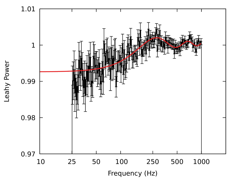
Figure 1: Deadtime model fitted to the NuSTAR data. See section 2.3 for details.

Finally, the Poisson noise corrected averaged power spectra are renormalized to squared fractional rms, and subsequently described in terms of a multi-Lorentzian model (Belloni et al., 2002). Each component, $L\left(\nu\mid r,Q,\nu_{\rm max}\right)$, is a function of Fourier frequency $\nu$ and characterized by three parameters. Here $\nu_{\rm max}=\nu_{0}\sqrt{1+1/4Q^{2}}$ is the characteristic frequency, and $Q=\nu_{0}/W$ the quality factor, where $\nu_{0}$ gives the centroid frequency and $W$ is the full-width-at-half-maximum. The amplitude of an individual component is expressed in terms of fractional rms, $r$, defined as

$$r^{2}=P=\int_{0}^{\infty}L(\nu)d\nu,$$

where $P$ is the integrated power. A component is considered to be significant if its integrated power has a single trial significance greater than three, that is, if $P/\sigma_{P}\geq 3$.

3 Results

Because the XMM-Newton and NuSTAR energy bands overlap, the XMM-Newton data is split in a low energy ($0.4-3$ keV) and high energy ($3-10$ keV) band, so that the latter is covered by both observatories, allowing for a direct comparison of their power spectra.

The first XMM-Newton observation (XMM-1) shows significant power in the $0.01$ to $10$ Hz frequency range (Figure 2, top panel). The integrated fractional rms amplitude is $24\%$ in the $0.4-3$ keV band, and increases to $43\%$ in the $3-10$ keV band.

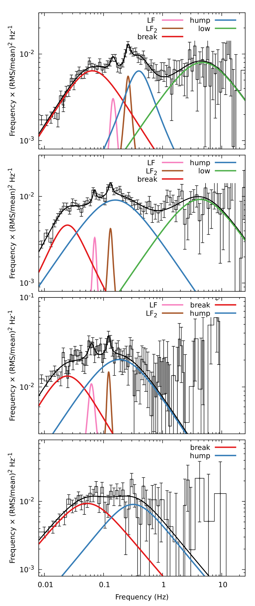
Figure 2: Power density spectra for the XMM-1 (top) and XMM-2 (second) data in the $0.4-3$ keV energy band, the NuSTAR-1 data (third), and the NuSTAR-2 data (bottom) in the $3-10$ keV energy band. Fit parameters are given in Table 3.

Table 1: Power spectrum fit parameters

Energy	Component	Frequency		Quality		Amplitude	$\chi^{2}$ / dof
(keV)		(Hz)				(% rms)
XMM-1
	break	0.065(6)	0.18(6)	13.1(6)
	hump	0.40(5)	0.8(3)	9.8(1
$0.4-3$	$\ell$ow	4.7(9)	0.  (fixed)	15.8(8)	70 / 81
	LF	0.146(5)	4.2(1.8)	3.3(5)
	$\mbox{LF}_{2}$	0.260(7)	4.3(1.1)	4.4(4)
	break	0.046(6)	0.35(11)	15.3(1
$3-10$	hump	0.29(2)	0.26(15)	23.4(1	104/87
	$\ell$ow	6.4(1	0.  (fixed)	28.5(1
XMM-2
	break	0.0245(18)	0.52(9)	9.4(9)
	hump	0.16(2)	0.  (fixed)	16.9(7)
$0.4-3$	$\ell$ow	4.3(7)	0.  (fixed)	17.0(8)	122 / 114
	LF	0.071(2)	6.4(26)	2.8(5)
	$\mbox{LF}_{2}$	0.131(3)	5.5(1.9)	3.4(4)
	break	0.026(3)	0.32(9)	18.7(2
$3-10$	hump	0.144(11)	0.27(13)	25.9(2	119 / 112
	$\ell$ow	3.3(6)	0.  (fixed)	31.0(1
NuSTAR-1
	break	0.024(4)	0.22(11)	19. (2)
$3-10$	hump	0.19(5)	0.  (fixed)	25.2(1	94 / 92
	LF	0.062(3)	3.6(1.7)	6.7(1
	$\mbox{LF}_{2}$	0.123(4)	6. (3)	6.0(1
$10-30$	break	0.041(6)	0.  (fixed)	28.2(1	86 / 77
NuSTAR-2
	break	0.05(2)	0.10(20)	16. (4)
$3-10$	hump	0.32(14)	0.  (fixed)	15. (5)	43 / 55
$10-30$	break	0.054(13)	0.  (fixed)	15.2(1	59/56

The $0.4-3$ keV power spectrum could be fitted with 5 Lorentzian components, three of which are broad noise terms and two are QPOs (see Table 3 for details). The centroid frequencies of the QPO differ by a factor of two within the measurement uncertainty, suggesting they are harmonically related.

While there is an indication the two QPOs are present in the harder $3-10$ keV energy band as well, the power spectrum could be adequately described using just three noise terms. These noise components are equivalent to the ones seen in the lower energy band, but have systematically larger amplitudes. Including the two QPOs with frequencies fixed at their previous position, however, does give a marginally significant detection. To determine if the QPOs are not independently resolved because their amplitudes drops relative to the band-limited noise terms, or because of a decrease in signal-to-noise I investigate the dependence of the power spectrum on energy in more detail.

Power spectra are constructed for 4 bands in the $0.4-10$ keV energy range. Each power spectrum is fit with the 5 component multi-Lorentzian model described above. To measure the energy dependence the amplitudes are left to vary while all other parameters are kept fixed. As shown in Figure 3 all five power spectral components show increasing amplitude as a function of energy. This indicates that the lower signal-to-noise in the $3-10$ keV band is due to the lower count rate, rather than a decrease is signal amplitude.

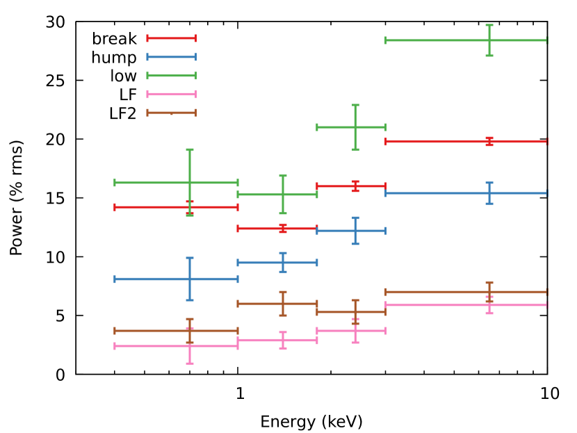
Figure 3: Lorenztian component rms amplitudes as a function of energy.

The second XMM-Newton observation (XMM-2) shows a similar power spectral shape as seen in the first observation, but with all features shifted to a slightly lower frequency and higher rms amplitude (Figure 2, second panel). The integrated power between $0.01$ and $10$ Hz in the $0.4-3$ keV band stands at $27\%$ rms. This power spectrum could again be fitted with a 5 component Lorentzian model, the details of which are shown in Table 3. The $3-10$ keV band shows a total integrated rms amplitude of $44\%$ rms, and could be adequately described with just the three broad noise terms.

For both XMM observations I also construct power spectra for light curve segment lengths of $\sim 1000$ seconds, so that the frequency range extends down to $\sim 1\times 10^{-3}$ Hz. However, neither observation shows additional power spectral features at very low frequencies.

For the first NuSTAR observation (NuSTAR-1) I first consider the $3-10$ keV energy band that is also covered by XMM-Newton. There is significant power between $0.01$ and $1$ Hz, with an integrated power of $\sim 40\%$ rms. There may be an additional feature $1$ Hz, however, the uncertainties there become to large to constrain the power density. The spectrum can be adequately fitted with two broad Lorentzian profiles and two QPOs (see Figure 2, third panel). The band-limited noise in the NuSTAR power spectrum is consistent with the two lower frequency noise terms seen in the XMM-2 observation. The two QPOs seen in the NuSTAR data again differ in frequency by a factor of two within their uncertainties. In terms of coherence and amplitude they are comparable to the QPOs seen in the XMM-Newton data, whereas their frequencies have slightly lower values.

In addition to the $3-10$ keV band I also construct power spectra for the $10-30$ keV energy band. In this higher energy band the power spectrum can be described using a single broad noise term, while no QPOs could be resolved.

The second NuSTAR observation (NuSTAR-2) has a higher count rate, but a much shorter exposure (30 vs 60 ks), such that the signal-to-noise ratio of this data is lower. The $3-10$ keV power spectrum can be adequately described with two broad noise terms (Figure 2, bottom panel). There is an indication of a narrow feature at $0.3$ Hz, but with a significance of $\leq 2\sigma$ it does not qualify as a detection.

4 Discussion

I have analyzed the X-ray variability of the accreting millisecond pulsar MAXI J0911 and found that the low frequency ($<10$ Hz) part of its power spectra can be described with two or three band-limited noise terms and two narrow QPOs.

4.1 Feature identification

The overall morphology of the power spectrum is reminiscent of an extreme island state atoll source (van der Klis, 2006). For such a state, the three noise terms may be identified as the break, hump, and $\ell$ow components, each having a progressively higher frequency. The two QPOs, seen atop the hump component, may then be identified as the Low-Frequency (LF) QPO and its harmonic (LF₂, van Straaten et al. 2003; Altamirano et al. 2005). The energy spectrum of MAXI J0911 is relatively hard (Sanna et al., 2017), which is consistent with an atoll source in this source state. The power spectral components, as shown in Table 3, have therefore been labeled according to this terminology.

A notable difference between MAXI J0911 and the wider class of atoll sources is that the frequencies measured in this work are about an order of magnitude lower than what is usually observed (see e.g. van Doesburgh & van der Klis 2017). Meanwhile, the observed fractional variability is remarkably high.

While extreme, these properties are in line with the source state evolution seen in atoll sources. As the energy spectrum increases in hardness, the power spectral features are observed to shift to lower frequencies, while broadening and increasing in amplitude (van der Klis, 2006). In this context the source state of MAXI J0911 would represent an outlier along the evolutionary track, suggesting that this system is accreting in a geometry not normally accessible by regular atoll type objects.

The identification of power spectral features in neutron star sources is usually confirmed by considering the frequency relations as a function of the highest frequency component in the spectrum. However, with the high frequency end of the power spectrum being poorly constrained, this is approach is not possible for MAXI J0911. Instead I test the frequency relation of the observed features with respect to the hump component. In atoll sources these features have nearly fixed frequency relations (van Straaten et al., 2002; Altamirano et al., 2008a), so that their frequency ratios are approximately constant (van Doesburgh & van der Klis, 2017). Hence the frequency ratios of the measured components relative to the hump component frequency are shown in Figure 4. While the absolute frequencies in MAXI J0911 are low, the frequency ratios are consistent with those in other atoll sources, and with those of other AMXPs as well. This strongly supports the identification of these features as LF QPOs.

An alternative interpretation of the QPOs may be that they are related the mHz QPOs (Revnivtsev et al., 2001), which are attributed to marginally stable burning of accreted material on the neutron star surface (Heger et al., 2007). While the luminosity of MAXI J0911 is in the regime where such QPOs are observed, there are several issues with this interpretations. Both the QPO frequencies and amplitudes in MAXI J0911 are higher by a factor of a few than is usual for mHz QPOs (Altamirano et al., 2008b; Linares et al., 2012), and so far no type I X-ray burst has been observed in MAXI J0911. More importantly, the QPO amplitudes show a steep increase as a function of energy, strongly disfavoring a scenario in which they originate from the neutron star surface.

Yet another possibility might be that periodic obscuration along the line of sight is giving rise to these QPOs. However, again, this seems unlikely. Dipping QPOs tend to have higher frequencies and amplitudes than what is observed in MAXI J0911 (Homan et al., 1999). What’s more, the rms amplitude of a dipping QPO is expected to be independent of energy, which does not correspond with the observations.

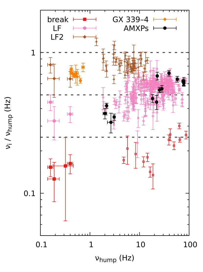
Figure 4: Frequency ratios $\nu_{i}/\nu_{\rm hump}$ as a function of the hump frequency, for MAXI J0911 (large solid symbols to the left) as compared to a sample of atoll sources (small open symbols). Orange symbols give the $\mbox{LF}_{2}$ frequencies measured in the black hole binary GX $339-4$, and black symbols give LF frequencies measured in other AMXPs.

4.2 IGR J00291+5934

There is only one other neutron star system that shows a power spectrum that is similar to the one observed in MAXI J0911. That source is the 599 Hz accreting millisecond pulsar IGR J00291+5934 (IGR J00291; Linares et al. 2007).

Observed with RXTE in the $2-20$ keV band, the power spectrum of IGR J00291 shows a $0.01-100$ Hz integrated power of $40-60\%$ rms (Linares et al., 2007). The break, hump, and low components all have comparable frequencies and amplitudes to those seen in MAXI J0911. Additionally, two very low frequency QPOs have been detected in IGR J00291. With frequencies of $22$ and $44$ mHz, however, they sit atop the break component rather than the hump component, and hence cannot be identified as LF QPOs such as those in MAXI J0911.

A very prominent 8 mHz flaring has also been detected in IGR J00291 (Ferrigno et al., 2017). This feature is not seen MAXI J0911, but if it is due to ‘heartbeat’ variability (Belloni et al., 2000; Altamirano et al., 2011), as suggested by Ferrigno et al. (2017), then such flaring may be a transient phenomenon and MAXI J0911 may in fact be a good candidate to monitor for such variability.

The similarity of their broadband power spectra can be taking to indicate that both MAXI J0911 and IGR J00291 are accreting in a comparable source state. That source state is then characterized by an highly energetic Comptonizing medium and a large fractional variability. As noted by Linares et al. (2007), these properties are naturally explained if the optically thick accretion disk is truncated at a relatively large radius. An extended inner flow would then set the high fractional amplitude and the energy dependence , while the comparatively cool outer disk sets the low dynamical frequency (Churazov et al., 2001; Gilfanov et al., 2003). How such a configuration would interact with the stellar magnetic field remains unclear (see Patruno et al. 2016 or a discussion).

There is no obvious observable parameter indicating why these particular sources would have a larger truncation radius, or more generally such an extreme source state. Both systems are millisecond pulsars, but have somewhat different properties (Sanna et al., 2017; Patruno, 2016). Their spin frequencies differ by nearly a factor of two. With an orbital period of $2660$ s MAXI J0911 is in a tighter orbit than IGR J00291, which has a period of $8844$ s. The mass limits on their companions is similar, and both have accretion have luminosities of $\sim 10^{36}$ erg s^-1 (Falanga et al., 2005; Sanna et al., 2017). However, the same can be said for other accreting millisecond pulsars. For instance, SAX J1808.4–3658 is more similar to IGR J00291 than MAXI J0911, and yet the power spectra of that SAX J1808.4–3658 are far more consistent with atoll sources at those luminosities (Bult & van der Klis, 2015).

Another peculiar property of MAXI J0911 is the duration of its outburst. Unlike IGR J00291, which shows a few week long outbursts every four to five years, MAXI J0911 has been continuously accreting for at least one year. From the two NuSTAR observations it follows that during this time the source state has remained unchanged. The only other AMXP to have shown such a long outburst is the 377 Hz intermittent pulsar HETE J1900.1–2455 (Kaaret et al., 2006), which remained active for about ten years. The power spectrum of that source, however, is that of a regular (extreme) island state atoll source (Papitto et al., 2013). This would suggest that neither intermittency nor outburst duty cycle has much bearing on the stochastic variability of these pulsars.

Potentially, the accretion geometry of MAXI J0911 and IGR J00291 can be accounted for by the detailed properties of the neutron star, depending on magnetic field strength, stellar mass, as well as the spin and magnetic alignment angles. While such properties are difficult to measure, detailed pulse profile modeling for IGR J00291 and MAXI J0911 may provide further clues.

4.3 The LF QPOs

The LF QPOs observed in MAXI J0911 have the lowest frequency seen in any accreting neutron star system. Instead their frequency range is more similar to those of the Low-Frequency QPOs observed in low-hard state black hole binaries (Klein-Wolt & van der Klis, 2008). This is illustrated in Figure 4, which also shows frequency ratios for the black hole binary GX $339-4$.

For black hole binaries there is strong evidence that LF QPOs (or type C QPOs in black hole terminology) are caused by Lense-Thirring precession (Ingram et al., 2016, 2017). In this model the accretion disk consists of two components; an inner, hot accretion flow emitting a hard Comptonized spectrum, and an outer thin disk emitting a softer thermal spectrum. If the black hole spin is misaligned with the accretion disk, frame dragging effects apply a torque on the hot flow, causing it to precess as a solid body (Ingram et al., 2009). This precession is argued to cause the LF QPOs. Qualitatively, this model is in good agreement with the power spectral features of MAXI J0911 and the hard energy spectrum of their amplitudes.

If neutron star systems have a precessing inner accretion flow like those predicted for black holes, then their LF QPO frequencies are not straightforwardly related to the Lense-Thirring precession frequency (Altamirano et al., 2012; Bult & van der Klis, 2015; van Doesburgh & van der Klis, 2017). For instance, in neutron star systems the stellar oblateness introduces an additional torque on the disk, giving rise to a retrograde precession term (Morsink & Stella, 1999). For accreting millisecond pulsars this situation is complicated further by the stellar magnetosphere, which truncates the accretion disk and has been proposed to introduces a third, magnetic torque (Lai, 1999; Shirakawa & Lai, 2002), leading to a second retrograde precession term.

Determining how, exactly, these various torques set the LF QPO frequency has the potential of yielding constraints on how the magnetosphere interacts with the disk, and of the neutron star properties itself. The black-hole like power spectrum of MAXI J0911 make this source an ideal target for such a study, for instance with the Neutron Star Interior Composition Explorer (NICER, Gendreau et al. 2012), which is scheduled for launch in 2017.

Appendix A Co-spectrum statistics

When a detector has more than one focal plane module, a single observation produces several concurrent time series. These time series may the be combined by either adding them, or by correlating them. In the following the statistical properties of each approach are derived and then compared.

A.1 Coherent averaging

Consider a discrete time series $x_{j}$ containing a total of $N_{\gamma}$ counts. It is well known that for a time series containing only Poisson noise, the elements of the Fourier transform, $X_{k}$, will be distributed as a complex normal variates with zero mean and variance $N_{\gamma}/2$ (Leahy et al., 1983). If I let

$$Z_{k}=\sqrt{\frac{2}{N_{\gamma}}}X_{k}=A_{k}e^{i\phi_{k}}+Z_{\rm noise},$$ (A1)

be a normalized Fourier transform of a signal in the presence of Poisson noise, then $A_{k}^{2}$ gives the signal Leahy power, $\phi_{k}$ is its underlying phase, while $Z_{\rm noise}$ is a complex-valued noise term with independent standard normal variates in both its real and imaginary parts.

Given an ensemble of $M$ concurrent measurements, the Fourier transforms can be averaged coherently (dropping the frequency index $k$ for convenience)

$$\left<Z\right>_{M}=Ae^{i\phi}+\left<Z_{\rm noise}\right>_{M},$$ (A2)

so that the variance reduces to $1/M$. By definition the sum of squared standard normal variates follows a chi-squared distribution. Similarly, the sum of squared normal variates that have a non-zero mean, $\mu_{n}$, and unit variance will follow a non-central chi-squared distribution, $\overline{\chi}^{2}(\nu,\lambda)$, characterized by $\nu$ degrees of freedom and non-centrality

$$\lambda=\sum_{n=1}^{\nu}\mu_{n}^{2}.$$ (A3)

It then follows that the power of $\left<Z\right>_{M}$ is distributed as $\overline{\chi}^{2}(2,MA^{2})$ scaled by a factor of $1/M$.

Given an ensemble of $L$ coherently averaged powers, the combined averaged power is distributed as

$$f_{P}(y)=\frac{1}{LM}\overline{\chi}^{2}\left(\frac{y}{LM}\mid\nu=2L,\lambda=LMA^{2}\right),$$ (A4)

which has a mean of

$$\mu_{P}=\frac{2}{M}+A^{2},$$ (A5)

and variance

$$\sigma^{2}_{P}=\frac{4+4MA^{2}}{LM^{2}}.$$ (A6)

Note that for a signal that is only averaged incoherently ($M=1$), eq. A4 reduces to the result derived by Groth (1975) for a signal in the presence of noise. For a pure noise signal ($A=0$) these results reduce further to the familiar chi-squared distribution with $2L$ degrees of freedom, and yields a Poisson noise level of $2$ (van der Klis, 1989).

A.2 Correlating concurrent series

For an ensemble of $M$ concurrent time series (as eq. A1) there are $\tilde{M}=\binom{M}{2}=\left(M-1\right)M/2$ unique pairs, each of which can be correlated to give an estimate of the co-spectrum. For such a pair, say $x_{a}[j]$ and $x_{b}[j]$, the co-spectrum at a particular frequency index is given as

$$C_{ab}=\mbox{Re}\left[Z_{a}Z_{b}^{*}\right]=R_{a}R_{b}+I_{a}I_{b},$$ (A7)

where $R_{a}$ and $R_{b}$ are normal variates with mean ${A\cos\phi}$ and unit variance. The terms $I_{a}$ and $I_{b}$ are similarly distributed with a mean of ${A\sin\phi}$. It is useful to define the product $Y_{ab}=R_{a}R_{b}$, for which the expectation and variance are given as

$$\mathbb{E}\left[Y_{ab}\right] =\mathbb{E}\left[R_{a}\right]\mathbb{E}\left[R_{b}\right]=A^{2}\cos^{2}\phi,$$

$$\mathbb{V}\left[Y_{ab}\right] =\mathbb{E}\left[R_{a}^{2}\right]\mathbb{E}\left[R_{b}^{2}\right]-\left(\mathbb{E}\left[R_{a}\right]\mathbb{E}\left[R_{b}\right]\right)^{2},$$

$$=1+2A^{2}\cos^{2}\phi.$$ (A8)

When averaging the product $Y$ over all $\tilde{M}$ correlation pairs the mean will reduce to this expectation. For the variance is important to realize that the pairs are not all independent. Specifically, the two products $Y_{ab}$ and $Y_{ac}$ have a covariance of

$$\mbox{Cov}\left[Y_{ab},Y_{ac}\right] =\mathbb{E}\left[R_{a}^{2}R_{b}R_{b}\right]-\mathbb{E}\left[Y_{ab}\right]\mathbb{E}\left[Y_{ac}\right],$$

$$=A^{2}\cos^{2}\phi.$$ (A9)

If I let $\Gamma_{nm}$ be the full covariance matrix of the $\tilde{M}$ correlation pairs, then the variance of the averaged product term will be

$$\mathbb{V}\left[\left<Y\right>_{\tilde{M}}\right] =\frac{1}{\tilde{M}^{2}}\sum_{m=0}^{\tilde{M}-1}\sum_{n=0}^{\tilde{M}-1}\Gamma_{nm}$$

$$=\frac{1}{\tilde{M}^{2}}\left\{\sum_{m=0}^{\tilde{M}-1}\Gamma_{mm}+\sum_{m=0}^{\tilde{M}-1}\sum_{\begin{subarray}{c}n=1\\ n\neq m\end{subarray}}^{\tilde{M}-1}\Gamma_{nm}\right\}$$

Each term in the first summation is given by eq A8. Because each of the $\tilde{M}$ pairs is correlated with $2(M-2)$ other pairs, the number of non-zero terms in the second sum is $M(M-1)(M-2)$, with each contribution given by eq. A9. The variance then reduces to

$$\mathbb{V}\left[\left<Y\right>_{\tilde{M}}\right]=\frac{1+2(M-1)A^{2}\cos^{2}\phi}{\tilde{M}}$$

The product $I_{a}I_{b}$ has similar averaged properties, but with the cosine terms replaced by sines. Since all sine and cosine terms are squared, it is easy to see how they drop out when the two averaged products are added to a single average co-spectrum.

Finally, considering an ensemble of $L$ separate observations, the co-spectrum estimator gives a mean and variance of

$$\mu_{C} =A^{2},$$ (A10)

$$\sigma_{C}^{2} =\frac{4+4(M-1)A^{2}}{LM(M-1)}$$ (A11)

A.3 Comparing convergence

Given a sample of $K$ observations with a two detector system I can distinguish three averaging scenarios. First, averaging in the time domain gives a standard deviation from eq. A6 using $M=2$ and $L=K$. Second, averaging by correlating in the Fourier domain gives a standard deviation from eq. A11 using $M=2$ and $L=K$. Third, averaging powers gives a standard deviation as in eq. A6 with $M=1$ and $L=2K$. For pure noise the ratios of these uncertainties relate as $1:\sqrt{2}:\sqrt{2}$, indicating that time domain averaging gives the best detection sensitivity, whereas correlating the concurrent time series gives the same sensitivity as combining their power spectra.

References

- Altamirano et al. (2012) Altamirano, D., Ingram, A., van der Klis, M., et al. 2012, ApJ, 759, L20
- Altamirano et al. (2008a) Altamirano, D., van der Klis, M., Méndez, M., et al. 2008a, ApJ, 685, 436
- Altamirano et al. (2005) —. 2005, ApJ, 633, 358
- Altamirano et al. (2008b) Altamirano, D., van der Klis, M., Wijnands, R., & Cumming, A. 2008b, ApJ, 673, L35
- Altamirano et al. (2011) Altamirano, D., Belloni, T., Linares, M., et al. 2011, ApJ, 742, L17
- Bachetti et al. (2015) Bachetti, M., Harrison, F. A., Cook, R., et al. 2015, ApJ, 800, 109
- Belloni et al. (2000) Belloni, T., Klein-Wolt, M., Méndez, M., van der Klis, M., & van Paradijs, J. 2000, A&A, 355, 271
- Belloni et al. (2002) Belloni, T., Psaltis, D., & van der Klis, M. 2002, ApJ, 572, 392
- Bildsten (1998) Bildsten, L. 1998, in NATO ASI Series, Vol. 515, The Many Faces of Neutron Stars, ed. R. Buccheri, J. van Paradijs, & A. Alpar, 419
- Bult & van der Klis (2015) Bult, P., & van der Klis, M. 2015, ApJ, 806, 90
- Churazov et al. (2001) Churazov, E., Gilfanov, M., & Revnivtsev, M. 2001, MNRAS, 321, 759
- Ducci et al. (2016) Ducci, L., Watanabe, K., Sanchez, C., et al. 2016, The Astronomer’s Telegram, 9738
- Falanga et al. (2005) Falanga, M., Bonnet-Bidaud, J. M., Poutanen, J., et al. 2005, A&A, 436, 647
- Ferrigno et al. (2017) Ferrigno, C., Bozzo, E., Sanna, A., et al. 2017, MNRAS, 466, 3450
- Gendreau et al. (2012) Gendreau, K. C., Arzoumanian, Z., & Okajima, T. 2012, in Society of Photo-Optical Instrumentation Engineers (SPIE) Conference Series, Vol. 8443, 13
- Gilfanov et al. (2003) Gilfanov, M., Revnivtsev, M., & Molkov, S. 2003, A&A, 410, 217
- Groth (1975) Groth, E. J. 1975, ApJS, 29, 285
- Harrison et al. (2013) Harrison, F. A., Craig, W. W., Christensen, F. E., et al. 2013, ApJ, 770, 103
- Hasinger & van der Klis (1989) Hasinger, G., & van der Klis, M. 1989, A&A, 225, 79
- Haskell & Patruno (2011) Haskell, B., & Patruno, A. 2011, ApJ, 738, L14
- Heger et al. (2007) Heger, A., Cumming, A., & Woosley, S. E. 2007, ApJ, 665, 1311
- Homan et al. (1999) Homan, J., Jonker, P. G., Wijnands, R., van der Klis, M., & van Paradijs, J. 1999, ApJ, 516, L91
- Homan et al. (2016) Homan, J., Sivakoff, G., Pooley, D., et al. 2016, The Astronomer’s Telegram, 8971
- Ingram et al. (2009) Ingram, A., Done, C., & Fragile, P. C. 2009, MNRAS, 397, L101
- Ingram et al. (2017) Ingram, A., van der Klis, M., Middleton, M., Altamirano, D., & Uttley, P. 2017, MNRAS, 464, 2979
- Ingram et al. (2016) Ingram, A., van der Klis, M., Middleton, M., et al. 2016, MNRAS, 461, 1967
- Kaaret et al. (2006) Kaaret, P., Morgan, E. H., Vanderspek, R., & Tomsick, J. A. 2006, ApJ, 638, 963
- Kennea et al. (2016) Kennea, J. A., Evans, P. A., Beardmore, A. P., et al. 2016, The Astronomer’s Telegram, 8884
- Klein-Wolt & van der Klis (2008) Klein-Wolt, M., & van der Klis, M. 2008, ApJ, 675, 1407
- Lai (1999) Lai, D. 1999, ApJ, 524, 1030
- Leahy et al. (1983) Leahy, D. A., Elsner, R. F., & Weisskopf, M. C. 1983, ApJ, 272, 256
- Leahy et al. (2008) Leahy, D. A., Morsink, S. M., & Cadeau, C. 2008, ApJ, 672, 1119
- Linares et al. (2012) Linares, M., Altamirano, D., Chakrabarty, D., Cumming, A., & Keek, L. 2012, ApJ, 748, 82
- Linares et al. (2007) Linares, M., van der Klis, M., & Wijnands, R. 2007, ApJ, 660, 595
- Morsink & Stella (1999) Morsink, S. M., & Stella, L. 1999, ApJ, 513, 827
- Papitto et al. (2013) Papitto, A., D’Aì, A., Di Salvo, T., et al. 2013, MNRAS, 429, 3411
- Patruno (2016) Patruno, A. 2016, ArXiv e-prints, arXiv:1611.06055
- Patruno et al. (2012) Patruno, A., Bult, P., Gopakumar, A., et al. 2012, ApJ, 746, L27
- Patruno et al. (2016) Patruno, A., Maitra, D., Curran, P. A., et al. 2016, ApJ, 817, 100
- Patruno & Watts (2012) Patruno, A., & Watts, A. L. 2012, in Timing neutron stars: pulsations, oscillations and explosions, ed. T. Belloni, M. Mendez, & C. M. Zhang (in press)
- Poutanen & Gierliński (2003) Poutanen, J., & Gierliński, M. 2003, MNRAS, 343, 1301
- Psaltis & Chakrabarty (1999) Psaltis, D., & Chakrabarty, D. 1999, ApJ, 521, 332
- Psaltis et al. (2014) Psaltis, D., Özel, F., & Chakrabarty, D. 2014, ApJ, 787, 136
- Revnivtsev et al. (2001) Revnivtsev, M., Churazov, E., Gilfanov, M., & Sunyaev, R. 2001, A&A, 372, 138
- Sanna et al. (2017) Sanna, A., Papitto, A., Burderi, L., et al. 2017, A&A, 598, A34
- Serino et al. (2016) Serino, M., Tanaka, K., Negoro, H., et al. 2016, The Astronomer’s Telegram, 8872
- Shirakawa & Lai (2002) Shirakawa, A., & Lai, D. 2002, ApJ, 564, 361
- van der Klis (1989) van der Klis, M. 1989, in NATO ASI Series, Vol. 262, Timing Neutron Stars, ed. H. Ögelman & E. P. J. van den Heuvel (Dordrecht: Kluwer), 27
- van der Klis (2006) van der Klis, M. 2006, in Compact stellar X-ray sources, ed. W. H. G. Lewin & M. van der Klis (Cambridge: Cambridge University Press), 39–112
- van Doesburgh & van der Klis (2017) van Doesburgh, M., & van der Klis, M. 2017, MNRAS, 465, 3581
- van Straaten et al. (2002) van Straaten, S., van der Klis, M., di Salvo, T., & Belloni, T. 2002, ApJ, 568, 912
- van Straaten et al. (2003) van Straaten, S., van der Klis, M., & Méndez, M. 2003, ApJ, 596, 1155
- van Straaten et al. (2005) van Straaten, S., van der Klis, M., & Wijnands, R. 2005, ApJ, 619, 455