Competition brings out the best: Modeling the frustration between curvature energy and chain stretching energy of lyotropic liquid crystals in bicontinuous cubic phases

Abstract.

It is commonly considered that the frustration between the curvature energy and the chain stretching energy plays an important role in the formation of lyotropic liquid crystals in bicontinuous cubic phases. Theoretic and numeric calculations were performed for two extreme cases: Parallel surfaces eliminate the variance of the chain length; constant mean curvature surfaces eliminate the variance of the mean curvature. We have implemented a model with Brakke’s Surface Evolver which allows a competition between the two variances. The result shows a compromise of the two limiting geometries. With data from real systems, we are able to recover the G–D–P phase sequence which was observed in experiments.

Keywords: Amphiphilic systems, Lyotropic liquid crystals, Bicontinuous cubic phases, Triply periodic minimal surfaces, Surface Evolver, Geometrical frustration

1. Introduction

Liquid crystals are called lyotropic if they experience phase transitions by adding or removing a solvent [Hil94]. Typically, the solute in a lyotropic liquid crystal (LLC) is amphiphilic, comprising a hydrophilic head-group and a hydrophobic chain (tail). Upon varying solvent content and/or temperature, LLC can display a rich variety of phases, including the lamellar phase, the hexagonal phase, and the bicontinuous or micellar cubic phases. Of these, the bicontinuous cubic phases are the most complex and interesting. They are observed in cells and organelles, and are believed to play important role in biological processes [AKD06]. It is generally believed that the bicontinous LLC cubic phases can be described by triply-periodic minimal surfaces (TPMS’s) [Scr76, LFK80, LM83, Mac85].

A LLC can be treated as a packing of curved amphiphile monolayers and water layers. According to the curvature of the monolayers (measured at the neutral interfaces [KW91, Tem95]), LLC can be classified into two types [LTGK⁺68, ST95, Hyd89]: With respect to normal vectors pointing from oil to water, the monolayers have positive mean curvature in a normal (a.k.a. type I, oil-in-water) system, and negative mean curvature in an inverse (a.k.a. type II, water-in-oil) system. In the case of a typical amphiphile-water binary LLC system, an inverse bicontinuous cubic phase consists of a pair of monolayers tail-to-tail (a bilayer) draped over the TPMS [SKM⁺07, SCT10, STFH06], separating two water channels; while in a normal phase, a water layer following the TPMS separates two channels packed by the hydrophobic tails of the amphiphiles [STFH06].

It is commonly believed that LLC phases arise from the competition between two geometric demands [Hel73, SC86, AGL88]: uniform curvature and uniform chain length in the monolayers. Indeed, as the amphiphilic molecules in the monolayers are chemically identical, it is conceivable that they have the same spontaneous curvature [Hyd90] and relaxed tail length. However, for most of the LLC phases, the curvature and the chain length can not be simultaneously uniform [DTS97, AGL88]. Hence the origin of frustration, which can be quantified by the variances of mean curvature and of chain length.

Considering both variances at the same time is difficult, hence most investigations treat them separately. The neutral interfaces are either modeled as parallel surfaces of the TPMS (e.g. [AGL88, TKS98, Hyd89, TSD⁺98, SG00b, SG01]), eliminating the variance of the chain length; then the Helfrich energy is calculated or measured as the energy of the system. Or, alternatively, the neutral interfaces are assumed to have constant mean curvature (CMC); then the Hooke energy is used as the energy of the system (e.g. [AGL88, SKM⁺07, SCT10, TSD⁺98, SG00a]). The parallel surface model is certainly more straight forward to calculate, but the CMC model makes more sense for the inverse hexagonal and micellar phases [AGL88, DTS97], and is arguably more successful in explaining the phase behaviour involving bicontinuous cubic phases [SCT10].

There has been a constant and strong demand [AGL88, SKM⁺07] for a model that allows the competition between the curvature energy and the chain stretching energy. Here we present a way of modeling LLC structures in Brakke’s Surface Evolver [Bra92] that fulfills this demand. We first demonstrate our method on the inverse hexagonal phase, then apply it to the bicontinuous cubic phases, both inverse and normal, with the geometry of G (gyroid, $Ia3d$), D (diamond, $Pn3m$), P (primitive, $Im3m$) TPMS’s. This gives, for the first time, a geometry of LLC that compromises the two extremes: the parallel surfaces and the CMC surfaces.

Acknowledgement

The authors appreciate discussions with Karsten Große-Brauckmann and Ken Brakke, and thank Gerd Schröder-Turk and Lu Han for feedbacks. Jin acknowledges the support of Corinna C. Maaß and Stephan Herminghaus.

2. Model

Following [SCT10], the surface averaged free energy per hydrophobic chain, denoted by $\mu$, comprises two parts:

(1) $$\mu=\mu_{C}+\mu_{L},$$

where

$$\mu_{C}=A(2\kappa_{H}\langle(H-H_{0})^{2}\rangle+\kappa_{G}\langle K\rangle)$$

is the Hilfrich energy or curvature energy [Hel73, FHL91], and

$$\mu_{L}=\kappa_{L}\langle(L-L_{0})^{2}\rangle$$

is the Hooke energy or chain stretching energy. Here, $A$ denotes the cross-sectional area of a hydrophobic chain, $L$ denotes the chain length, $H$ is the interfacial mean curvature, $K$ is the interfacial Gaussian curvature, $H_{0}$ is the spontaneous mean curvature, $L_{0}$ denotes the relaxed chain length, and $\kappa_{H}$, $\kappa_{G}$ and $\kappa_{L}$ denote the moduli for the energetic contributions from, respectively, the mean curvature, Gaussian curvature, and hydrophobic chain stretching. All these quantities should be measured on or from the neutral interface, which is the location within the monolayer where the area is invariant upon isothermal bending [KW91, Tem95]. The average is over the whole surface, that is $\langle x\rangle=\int_{S}xdS/\int_{S}dS$.

The contribution from the mean curvature can be rewritten as

(2) $$2A\kappa_{H}\left<(H-H_{0})^{2}\right>=2A\kappa_{H}\left[(\langle H^{2}\rangle-\langle H\rangle^{2})+(\langle H\rangle-H_{0})^{2}\right]=2A\kappa_{H}\sigma_{H}^{2}+\bar{\mu}_{H}$$

where $\sigma_{x}=\langle x^{2}\rangle-\langle x\rangle^{2}$ denotes the squared variance. Similarly, the contribution from the chain stretch can be decomposed into

(3) $$\mu_{L}=\kappa_{L}\left[(\langle L^{2}\rangle-\langle L\rangle^{2})+(\langle L\rangle-L_{0})^{2}\right]=\kappa_{L}\sigma_{L}^{2}+\bar{\mu}_{L}.$$

The frustration of the system is measured as a weighted sum of the squared variances

$$2A\kappa_{H}\sigma_{H}^{2}+\kappa_{L}\sigma_{L}^{2},$$

which is the quantity to minimize in our model.

This model is certainly a simplification. In particular, we ignore the contribution of the tilt energy (which will be justified later), the higher order contributions of the curvatures, as well as the non-local interactions of the monolayers, such as van der Waals interaction and hydration repulsion. Nevertheless, it is hoped that the important physical features are retained.

Brakke’s Surface Evolver [Bra92] is a software that minimizes energies of triangulated surfaces subject to constraints and boundary conditions. Apart from the usual surface tension energy, or the area functional, Surface Evolver is able to calculate many other quantities on a surface. Many of these quantities can be included in the energy to minimize. A quantity can be calculated on a particular set of geometric elements (vertices, edges, faces, bodies), allowing the users to control which elements contribute to the total energy. Moreover, each quantity has a modulus to specify its weight in the total energy. The moduli are adjustable in real time on each geometric element.

In particular, Surface Evolver has implemented the Willmore energy $(h-h_{0})^{2}$ (see [HKS92]) evaluated on vertices, and the Hooke energy $(\ell-\ell_{0})^{2}$ evaluated on edges. Here, we use lower case letters to distinguish dimensionless quantities in Surface Evolver from physical quantities. More specifically, our computations in Surface Evolver assume unit lattice parameter (edge length of the conventional cubic cell of the TPMS). If the physical system has lattice parameter $a$, we have the relations $h=Ha$, $k=Ka^{2}$ and $l=L/a$. Then the surface averaged energy per hydrophobic chain takes the following form

(4) $$\mu=Aa^{-2}\left[2\kappa_{H}\langle(h-h_{0})^{2}\rangle+\kappa_{G}\langle k\rangle\right]+\kappa_{L}a^{2}\langle(\ell-\ell_{0})^{2}\rangle.$$

The parameters $h_{0}$ and $\ell_{0}$ in Surface Evolver are supposed to mean the dimensionless spontaneous mean curvature and relaxed chain length. However, we keep updating these parameters to the average values $\langle h\rangle$ and $\langle\ell\rangle$, so that the averaged Willmore energy gives the squared variance of mean curvature, and the averaged Hooke energy gives the squared variance of chain length. Hence the minimized quantity is the frustration

$$2A\kappa_{H}a^{-2}\sigma_{h}^{2}+\kappa_{L}a^{2}\sigma_{\ell}^{2}$$

or, for convenience,

$$\sigma_{h}^{2}+\lambda\sigma_{\ell}^{2}$$

where $\lambda=\kappa_{L}a^{4}/2A\kappa_{H}$. After sufficiently evolving the surface, it is easy to transform the minimized frustration into the energy using Eqs. (2) and (3).

Our procedure of modeling bicontinuous LLC cubic phases in Surface Evolver can be outlined in the following five steps.

1. Prepare a triangulation of the D, P or G surface, or any other surface of interest.

2. Make two copies of the triangulation, modeling the neutral interfaces. Assign Willmore energy to these copies.

3. Create edges modeling the hydrocarbon chains, and assign Hooke energy to these edges.

4. Impose a volume constraint to the space between the neutral interfaces in correspondance with the desired water fraction.

5. Evolve the surface towards the minimum of the total energy, while keep updating the average values $h_{0}=\langle h\rangle$ and $\ell_{0}=\langle\ell\rangle$.

In step (3), the edges modeling the hydrophobic chains depend on the system and the model. For inverse LLC phases, we are aware of several ways of modeling the chains:

1. Connect edges between the corresponding vertices on the triangulated neutral interfaces.

2. Connect edges from the vertices on the neutral interfaces to the corresponding vertices on the TPMS.

3. Subtending normal vectors from the TPMS until the neutral interfaces (used in [SKM⁺07]).

4. Subtending normal vectors from the neutral interfaces until the TPMS.

In order to consider the curvature and the chain length at the same time, we need to keep the chains up to date at every step of surface evolution. The models (c) and (d) require computing the intersection point of a line and a triangulated surface, which is very time consuming. We will use the models (a) and (b). The chains are established once at the beginning, and will be used during the entire computation.

However, only the model (d) forces the chains to be perpendicular to the neutral interfaces. This may raise concerns on the legitimacy of ignoring tilt energy (see [HK00]) in other models. We address to this concern by measuring the amount of tilting. It turns out that the chains do not tilt much, at least in the inverse bicontinuous cubic phases, thanks to the normal_motion mode of the Surface Evolver.

An edge in the model (a) corresponds to two chains. One advantage of this model is that it is independent of the TPMS: the TPMS is present only for reference, and does not participate in the calculation. Our program is robust in the sense that, if one starts from a periodic CMC surface instead of a TPMS (which the author did, accidentally), the bilayer will correctly evolve to the TPMS. Hence our program confirms, under the current theory, that bicontinuous LLC cubic phases do follow the geometry of TPMS.

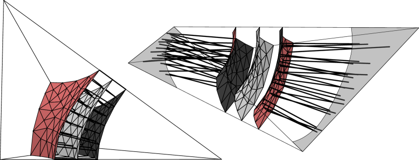
Figure 1. Our Surface Evolver models illustrated for the P phase. A triangulation of the P patch (light grey) is copied twice. The copies (red and dark grey) model the neutral interfaces. The black bold segments are the edges modeling the hydrophobic chains. Left: model (a) for the inverse LLC P phase, with hydrophobic chains connecting corresponding vertices on the neutral interfaces. Right: model for the normal LLC P phase, with hydrophobic chains connecting the neutral interfaces to the medial surface (grey area).

For normal LLC phases, we subtend normal vectors from vertices of the triangulated TPMS to find intersection points on the medial surface, then model the hydrophobic chains by edges from these intersection points to the corresponding vertices on the neutral interfaces. This model follows the idea of [SRCH03]. See Figure 1 for an illustration of our models.

The readers are free to use other chain models in their own calculations. The technical details are postponed to Section 5.

3. Result

3.1. Inverse hexagonal phase

In the inverse hexagonal LLC phase, water is contained in the tubes formed by amphiphiles arranged in a hexagonal lattice. Due to its simplicity, the inverse hexagonal phase has been a standard example (e.g. [DTS97, AGL88]) to illustrate the incompatibility between uniform curvature and uniform chain length, and to demonstrate the calculation of chain frustration within the CMC model.

We also choose the hexagonal phase to explain our method, since the model can be built up in dimension $2$. More specifically, the hexagonal lattice graph plays the role of TPMS, and a “triangulation” is nothing but a subdivision of the edges. The neutral interfaces are modeled by cycles within the hexagonal cells. In practice, such a cycle is initially created as a copy of the hexagon. Vertices of the cycles are connected to the corresponding points on the hexagonal lattice graph, modelling the hydrophobic chains of the amphiphiles (model (b)). The area between the cycle and the hexagon corresponds to half of the volume between the neutral interfaces.

Surface Evolver is able to apply squared curvature energy on the cycle, and Hooke energy on the hydrophobic chains. We can choose to minimize either energy alone, or minimize a weighted sum of the two. At each iteration, we update the parameter $\ell_{0}$ to the average chain length, so that the averaged Hooke energy actually gives the dimensionless squared variance of chain length. Note that the average curvature is a constant here.

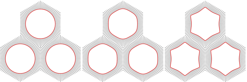
Figure 2. Evolved results of our model applied to the inverse hexagonal phase by minimizing only the curvature energy (left), only the chain stretching energy (right), and the frustration as a weighted sum of the two (middle). The cycles in red model the neutral interfaces, and the segments in grey model the hydrophobic chains (model (b)).

In Figure 2, we show the result of Surface Evolver under three different situations. Minimizing curvature energy alone results in a circle, and minimizing chain stretching energy alone results in a star-like shape. If both are present in the total energy, a competition arise. The cycle evolves to a closed curve, which is neither a circle nor a star, but an intermediate shape.

3.2. Inverse LLC phases

We now repeat the calculation of Shearman et al. [SKM⁺07] to verify the feasibility of our method. More specifically, we measure the chain frustration in inverse LLC phases assuming CMC neutral interfaces. The hydrophobic chains are modeled by edges connecting corresponding vertices on the triangulated neutral interfaces; recall that they are copies of the same triangulation. The chain lengths are then half of the edge lengths. The volume fraction $\phi_{n}$ of the space between the neutral interfaces ranges from $0.01$ to $0.50$. The squared variance $\sigma_{\ell}^{2}$ of dimensionless chain length is measured as the frustration of the system.

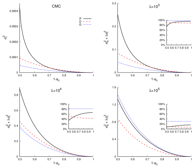
Figure 3. Frustration of the inverse D, P and G phases against $1-\phi_{n}$. Top-left: squared variance of chain length of the CMC model, to compare with [SKM⁺07]. Other: Weighted sum of the squared variances with $\lambda=10^{3}$, $10^{4}$ and $10^{5}$. The insets show the contribution of the squared variance of chain length in the total frustration.

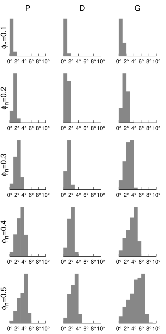
Figure 5. Histograms of chain tilt angles in the inverse bicontinuous cubic phases with different $\phi_{n}$.

The result is plotted in the top-left panel of Figure 3. We use $1-\phi_{n}$ on the $x$-axis to facilitate the comparison with Figure 5 in [SKM⁺07]. The two plots are very similar: The frustration is the lowest in the G phase, and the highest in the P phase when the water fraction is low, or in the D phase when the water fraction is high. In particular, we also observe a crossover between the P and D phases around $\phi_{n}=0.29$ ($\approx 0.25$ in  [SKM⁺07]). There is only a slight numerical disagreement, which can be explained by the minor differences in our models. In particular, the hydrophobic chains in [SKM⁺07] is perpendicular to the TPMS, while we allow slight tilting for the chains.

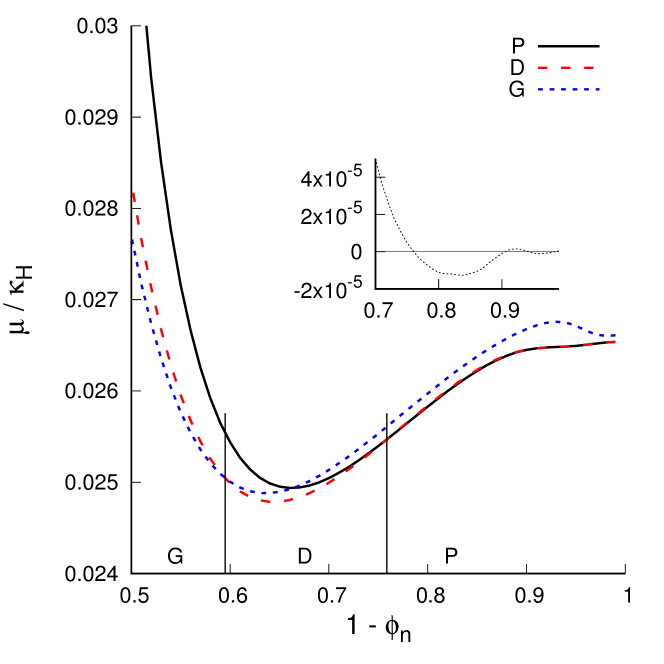
Figure 8. Surface averaged energies per hydrophobic chain divided by $\kappa_{H}$ of inverse D, P and G are plotted against $1-\phi_{n}$, with $A=33\text{\AA}^{2}$, $\kappa_{G}/\kappa_{H}=-0.75$, $\kappa_{L}/\kappa_{H}=0.00035\text{\AA}^{-2}$, $H_{0}=1/62.8\text{\AA}^{-1}$ and $L_{0}=8.8\text{\AA}$. With the increasing $1-\phi_{n}$, the phase with the lowest energy gives the sequence G–D–P. The inset shows the energy difference of P over D at $1-\phi_{n}$ larger than $0.7$.

Now that we have confirmed the validity of our algorithm, we turn on the Hooke energy in Surface Evolver, and minimize the weighted sum of the two dimensionless squared variances. We fix the weight of $\sigma_{h}^{2}$ to be $1$, and vary the weight of $\sigma_{l}^{2}$. In other words, we are minimizing $\sigma_{h}^{2}+\lambda\sigma_{\ell}^{2}$, corresponding to the frustration divided by $2A\kappa_{H}a^{-2}$. In view of parameter values provided in [SCT10], we choose $\lambda=10^{3}$, $10^{4}$, $10^{5}$ in our computations; see context of Figure 8. The result surface is neither parallel nor constant mean curvature, but a compromise of the two. The measured frustrations, together with the contribution of chain length frustration, is plotted in Figure 3. Histograms in Figure 5 show tilt angles less than $10$ degrees, justifying our practice of ignoring the tilt energy.

The mean curvature and the chain length compete to be uniform, and a higher weight is an advantage in this competition, hence the value of $\sigma_{\ell}^{2}$ is lower comparing to the CMC model. Moreover, the contribution of $\lambda\sigma_{\ell}^{2}$ in the total frustration is decreasing as $\lambda$ increases. This trend is more significant in the D and P phases than in the G phase. As a consequence, the frustration in the G phase eventually surpasses the D and P phases when $\lambda=10^{5}$.

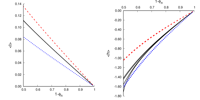
Figure 4. The dimensionless average chain length $\left<\ell\right>$ (left) and average mean curvature $\left<h\right>$ (right) of inverse bicontinuous cubic phases. The plots with CMC, $\lambda=10^{3}$, $\lambda=10^{4}$ and $\lambda=10^{5}$ are overlapped to emphasize on their similarity.

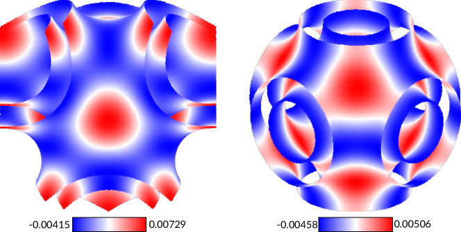
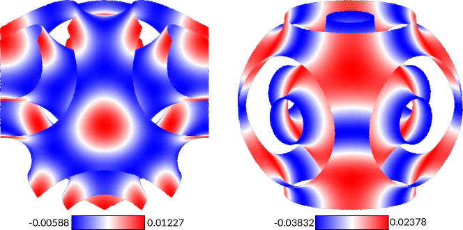
Figure 6. Evolved neutral interfaces in the inverse D (left) and P (right) phases with $\lambda=10^{4}$, and the space between the neutral surfaces, which is completely occupied by hydrophobic chains, has a volume fraction $\phi_{n}=0.3$ (top) or $\phi_{n}=0.5$ (bottom). The color shows the difference from the CMC surface with the same $\phi_{n}$: red indicates a deviation away from the TPMS, and blue indicates a deviation towards the TPMS. The color bar below each figure shows maximum deviations, normalized with unit lattice parameter. Clearly, the competition causes expansions in the necks.

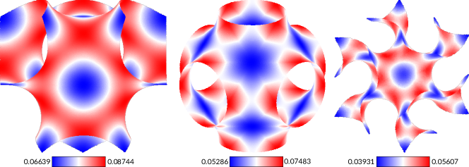
Figure 7. The D(left), P(middle) and G(right) TPMS color by its distance to the CMC neutral surfaces with $\phi_{n}=0.3$. The color bar shows the minimum and maximum distance, normalized with unit lattice parameter. This plot is a reproduction of Figure 8 of  [SKM⁺07].

As an example, the evolved P and D neutral interfaces with $\phi_{n}=0.3$ or $0.5$ and $\lambda=10^{4}$ are shown in Figure 6. The difference of the resulting neutral interfaces from the CMC interfaces with the same volume fraction $\phi_{n}$ is not visible with human eyes. This is also observed in Figure 4 where plots of average chain length and average mean curvature are overlapped to show the similarity. We then use CloudCompare [GM⁺16] to measure the deviation from the CMC interfaces, and color the surface accordingly for visualization. Roughly speaking, comparing to the CMC model, the neutral interfaces tend to move away from the TPMS around the flat points (where Gaussian curvature vanishes) of the TPMS, and towards the TPMS at other places. This is compatible with the observation in the CMC model that the chains are compressed around the flat points of the TPMS, and extended other where; see Figure 8 of [SKM⁺07], or Figure 7 for a colorful reproduction.

If the water fraction decreases further, the neutral interfaces in the CMC model tends to spheres (positive Gaussian curvature) connected by small necks (negative Gaussian curvature) [ADNS87, GB12]. Eventually, there will be a pinch-off point due to certain physical threshold, e.g., molecular size, and the bicontinuous phases are substituted by micellar phases. For the P phase, the pinch-off is supposed to occur at $\phi_{n}=0.5$ [SKM⁺07]. This can be observed in the top-left panel in Figure 3, as the curve for the P phase becomes very sloped near $\phi_{n}=0.5$. However, water fraction in experiment can be much smaller [SCT10]. This inconsistency is a weak point of the CMC model. In our model, the plot curve becomes less sloped, implying that the pinch-off point is moving towards lower water fraction. Indeed, we see in Figure 6 that the competition causes expansions in the necks, therefore delays the pinching off. Hence our model is able to cover highly dehydrated LLCs observed in experiment, which can not be explained by the CMC model [SCT10, TKS98].

Calculations shown in Figure 3 assume constant modulus, thus do not correspond to any experimental systems. To connect to the real systems, we need to know the lattice parameter $a$. Recall that the surface averaged energy per hydrophobic chain divided by $\kappa_{H}$, expressed with dimensionless quantities, is

$$\frac{\mu}{\kappa_{H}}=\frac{A}{a^{2}}\left[2\left<(h-h_{0})^{2}\right>+\frac{\kappa_{G}}{\kappa_{H}}\left<k\right>\right]+\frac{\kappa_{L}a^{2}}{\kappa_{H}}\left<(\ell-\ell_{0})^{2}\right>.$$

The total Gaussian curvature $\int_{S}kdS$ is a topological constant $2\pi\chi$, where $\chi$ is the Euler characteristic of the TPMS in the conventional cubic unit. The value of $\chi$ is $-4$ for the P surface, $-2$ for the D surface and $-8$ for the G surface. A relation between $a$ and $\phi_{n}$, as well as typical ranges for other parameters, are available in [SCT10]. We take the values $A=33\text{\AA}^{2}$, $\kappa_{G}/\kappa_{H}=-0.75$, $\kappa_{L}/\kappa_{H}=0.00035\text{\AA}^{-2}$, $H_{0}=1/62.8\text{\AA}^{-1}$. As for the relaxed chain length, we take for the moment $L_{0}=8.8\text{\AA}$, which is the measured distance from the chain ends to the neutral interface in the G phase [CC94] of $1$-monoolein/water system. These allow us to plot $\mu/\kappa_{H}$ in Figure 8 as a function of $1-\phi_{n}$. The phases of lowest energy gives a G–D–P sequence with increasing water fraction, which is a widely observed phase sequence in experiments [TKR98, TMS06] (see also [QC00]). The energy compositions of different phases are plotted in Figure 9.

However, the readers should be warned that the relation between $a$ and $\phi_{n}$, as well as some parameter values we use in this calculation, is derived under the CMC model. Our result is indeed very close to the CMC model. For instance, there is no visible difference in the dimensionless average chain length; see Figure 4. However, the difference may become significant with low water fraction. In the right panel of Figure 4, the plots of average mean curvature divert near $\phi_{n}=0.5$. When $\phi_{n}=0.5$, the deviation of the evolved neutral interfaces from CMC interfaces is comparable with the chain length; see bottom of Figure 6. Hence the usability of these parameter values is subject to further verification.

3.3. Normal LLC phases

LLC in normal bicontinuous cubic phases seem to be less common. The authors are not aware of any reports other than normal bicontinuous G phase [SS97, AOL98]. Meanwhile, in mesophased silica system, which can be seen as LLC systems with water replaced by silica, various normal phases have been reported, including the bicontinuous G [MSH⁺93, And97, AET⁺05], P [JTH⁺05] and D [GSS⁺06] phases.

Despite of our limited understanding, we repeat the same calculations to the normal bicontinuous LLC cubic phases, with the volume fraction $\phi_{n}$ of the space between the neutral interfaces (containing water) ranging from $0.01$ to $0.50$. Following Schröder-Turk et al. [SRCH03, STFH06], the hydrophobic chains are modeled by edges from vertices on the triangulated neutral interfaces along the normal vectors to the nearest point on the medial surface of the TPMS.

Because of the way that Surface Evolver calculates the volume, the measurements near $\phi_{n}=0$ are not physically meaningful; see Section 5. The tilt angles are much larger than in the inverse phases, hence the tilt energy is not really ignorable; see histograms in Figure 12. Hence we do not attempt to connect our calculation with real system. For these reasons, and also due to lack of CPU power, we only compare the CMC model with the case $\lambda=10^{4}$.

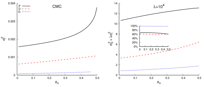
Figure 10. Frustration of the inverse D, P and G phases against $1-\phi_{n}$. Left: Squared variance of chain length of the CMC model. Right: Weighted sum of the squared variances of our model with $\lambda=10^{4}$. The inset shows the contribution of the squared variance of chain length in the total frustration.

The measured frustrations for the P, D and G phases, as well as the contribution of chain stretching energy when $\lambda=10^{4}$, are plotted in Figure 10. In both CMC model and our model, the frustration is the highest in the P phase and the lowest in the G phase. This could explain the difficulty of observing the normal bicontinuous P and D phases in experiment. As in the inverse phases, we see that the value of $\sigma_{\ell}^{2}$, as well as the contribution of $\lambda\sigma_{\ell}^{2}$, declines as $\lambda$ increases. The effect is again more significant in the D and P phases than in the G phases.

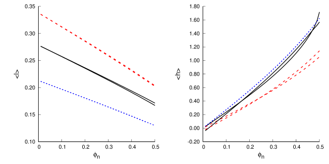
Figure 11. The dimensionless average chain length $\left<\ell\right>$ (left) and average mean curvature $\left<h\right>$ (right) of normal bicontinuous cubic phases. The plots with CMC and $\lambda=10^{4}$ are overlapped to emphasize on their similarity.

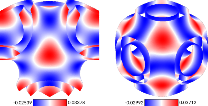
Figure 13. Evolved neutral interfaces in the normal D (left) and P (right) phases with $\lambda=10^{4}$, and the space between the neutral surfaces, which contains the water, has a volume fraction $\phi_{n}=0.3$. The color shows the difference from the CMC surface with the same $\phi_{n}$: red indicates a deviation away from the TPMS, and blue indicates a deviation towards the TPMS. The color bar below each figure shows maximum deviations, normalized with unit lattice parameter. Clearly, the competition causes expansions in the necks.

Plots of average chain length and average mean curvature are overlapped in Figure 11, showing the geometric similarity between CMC model and our model. Evolved D and P bilayers with $\phi_{n}=0.3$ are shown in Figure 13, to compare with Figure 6. Again, the neutral interfaces tend to move away from the TPMS around the flat points, and towards the TPMS at other places. Indeed, the flat points of the TPMS are most distant from the medial surface [SRCH03]. As a consequence, the pinching off necks gets expanded. Comparing to the inverse phases, the deviation is much larger ($>3\%$ of the lattice parameter).

4. Conclusion

We have demonstrated that modeling the competition between the curvature energy and the chain stretching energy in LLC systems is possible with Surface Evolver. More specifically, we applied Willmore energy to triangulated surfaces modeling the neutral interfaces, and Hooke energy to edges modeling the hydrophobic chains. A weighted sum of the two is used as the total frustration of the system, and is minimized by Surface Evolver. The resulting surfaces are neither parallel surfaces nor CMC surfaces, but a compromise of the two. A detailed procedure is described and tested for LLCs in bicontinuous cubic phases.

We compare our results on inverse cubic LLC phases to similar calculations with the CMC model [SKM⁺07]. The squared variance of chain length, as well as its contribution of the total frustration, is reduced as the modulus of chain stretching energy increases. This effect is more significant in the P and D phases than in the G phase. The frustration of the inverse G phase eventually exceeds the inverse D and P phases. A closer look reveals that the pinching off necks in the CMC model, which was the main obstacle to achieve a high dehydration [SCT10, TKS98], get expanded in our model. These observations prove the validity and usefulness of our model. When real data is applied, our calculation yields a G–D–P phase sequence with increasing water fraction, which has been observed in experiments. We also performed same calculations on normal cubic LLC phases. Similar observations are made, but the deviation from the CMC model is much more significant than in the inverse phases.

5. Technical details

In the opinion of the authors, the modelling capacity of Surface Evolver is underestimated. One purpose of this paper is to present a non-trivial application of Surface Evolver in the study of interfaces. In this section, we provide details of our calculation on bicontinuous LLC cubic phases, as a reference for readers who are interested in carrying out similar computations.

5.1. Surface preparation

The cubical periodic minimal surfaces considered in this paper, namely Schwarz’ G, D and P surfaces, can be generated from a small “fundamental patch” (Flächenstück) by Euclidean motions like translations, reflections, rotations and rotoreflections. However, only translations and reflections apply to the accompanied neutral interfaces that are of physical interests. Reflectional symmetries are related to free boundary conditions, and translational symmetries to periodic boundary conditions. Rotational symmetries are often related to fixed boundary conditions, but the neutral interfaces do not subject to any fixed boundary condition. Hence we only consider the fundamental unit of the translational and reflectional symmetries.

For the P and D surfaces, the .fe datafiles are available on Brakke’s website (http://facstaff.susqu.edu/brakke/evolver/examples/periodic/periodic.html). The P patch in the datafile is directly usable. We have to apply a rotation to the D patch to obtain the desired unit. For the G surface, we use a $96$-facets datafile kindly provided by Große-Brauckmann; see [GB97]. The G surface has no reflectional symmetry, hence the fundamental unit is a translational unit cell. In Surface Evolver, the torus model is used for the G surface to impose periodic boundary condition.

After loading the datafile into Surface Evolver, we use the command r (refine) to subdivide each triangle into four and, after each refinement, evolve the surface towards the minimum of the area functional. A translational unit cell is not a minimizer of the area functional, unless a volume constraint is imposed [GBW96], which we did for the G surface. Apart from the command g that performs one iteration of gradient descent, the command hessian_seek applies Newton–Raphson method to the gradient of energy. It is more efficient, yet safer than the more radical hessian command.

As in [SCT10], the P patch is refined four times, yielding $1024$ faces per patch; and the D patch is refined five times, yielding $2048$ faces per patch. Due to lack of CPU power, we only refine the G surface three times, yielding $6144$ faces per unit cell. Surface Evolver provides commands to eliminate elongated triangles (K) and extreme edges (l and t), as well as commands for vertex averaging (V) and equitriangulation (u). They are frequently employed to keep the triangulation in good shape.

Surface Evolver is very good at preparing triangulations. But if an exact formula is known for the surface of interest, one could also use a mesh generator to produce a triangulation of high quality; see for instance [SRCH03].

5.2. Setting up the bilayer

Now that we are in possession of a triangulation of high quality, we make two copies of it to model the neutral interfaces. The commands new_vertex, new_edge and new_facet are useful in this step. We also use element attributes to remember the correspondence between the elements in the original triangulations and in the copies.

To model an inverse phase, we only need to create edges between the corresponding vertices in the copied triangulations (model (a) as illustrated on the left of Figure 1). The edge length is thus twice the length of the chain we intend to model. This practice aims to eliminate the interference of the original TPMS in our calculation. After creation of the chains, The TPMS is fixed, and serves only as a reference. This procedure also works on unbalanced TPMS, such as the I-WP surface.

To model a normal LLC phase, we need to find, for each vertex in the triangulated TPMS, the nearest point on the medial surface along the normal vector. Efficient algorithms for this purpose based on Voronoi diagram was proposed by Amenta et al. [ACK01] and Schröder et al. [SRCH03]. In particular, [SRCH03] contains an extremely detailed description of the medial surfaces of the D, P and G surfaces, accompanied by fantastic figures. The medial surface of the P surface is very simple: they are contained in the reflection planes. Hence we simply attach one end of the edge to a vertex $v$ on the P surface, extend the edge along the normal vector at $v$ (available in the vertex_normal attribute), and attach the other end to the first point we encounter on the reflection plane. The same practice also yields a good approximation for the medial surface of the D surface.

For the G surface, we implement with Scipy a slightly simplified version of the algorithm in [ACK01]. For a vertex of the triangulated G surface, we choose from its Voronoi cell the vertex with the largest inner product with its normal vector. This is a good approximation of the “pole” in [ACK01], which is defined as the furthest vertex of the Voronoi cell. Scipy computes Voronoi diagrams using the Qhull library [BDH96].

Setting up for the inverse phases is automated with the script language of Surface Evolver. Automation for the normal phases is possible with exterior programs.

5.3. Minimization and measurement

In Surface Evolver, The Hooke energy $(\ell-\ell_{0})^{2}$ is implmented as hooke_energy. The quantity star_perp_sq_mean_curvature is a robust implementation of the Willmore energy $(h-h_{0})^{2}$; see [HKS92]. The Willmore energy is internally weighted by the effective area of each vertex, which is $1/3$ of the total area of facets containing the vertex. The parameters $h_{0}$ and $\ell_{0}$ are meant to be the spontaneous mean curvature and the relaxed length. We keep updating them to the average values $\langle h\rangle$ and $\langle\ell\rangle$ so that the energies measure the squared variances. The surface tension energy is turned off (set facet tension 0).

The moduli of the energies are also used for taking averages and normalizations. Let $\kappa_{L}$ and $\kappa_{H}$ be the experimental moduli for the chain stretching and mean curvature energy, respectively. Then in Surface Evolver, the modulus for the chain stretching energy is $k_{L}a^{2}A_{v}/a_{0}^{2}A$ at vertex $v$, and the modulus for the curvature energy is $k_{H}a_{0}^{2}/Aa^{2}$ for the dimensionless squared variance. Here, $A$ is the total area; $A_{v}$ is the effective local area of the vertex $v$; $a$ is the experimental lattice parammeter; $a_{0}$ is the lattice parameter in Surface Evolver model, which is $2$ for the P and D surfaces, and $8$ for the G surface. Recall that the Willmore energy is internally weighted by effective area, hence a factor $1/A$ suffices for normalization.

Let $\phi_{n}$ be the desired fraction of the space between the neutral interfaces. We impose a volume constraint of value $\phi_{n}V$ to the body bounded by the neutral interfaces. Here $V$ is the volume of the fundamental unit, which is $1/6$ for P, $2/3$ for D and $256$ for G surface. For normal phases, the neutral interfaces may intersect when $\phi_{n}$ is close to $0$. This is physically impossible, but not a numerical mistake. Surface Evolver computes volume by vector integration on the bounding faces. In our situation, the integrations on the two neutral interfaces have opposite signs, and they cancel to the imposed small volume. As $\phi_{n}$ increases, the neutral interfaces will be separated very soon.

In practice, the volume fraction $\phi_{n}$ is changed gradually in steps of $0.01$. The small changes not only ensure a precise measurement, but also avoid brutal changes in the surface that could destroy the surface. After each step, the surface is evolved (by commands g and hessian_seek) towards the minimum of the total energy. To measure the dimensionless squared variances, the parameters $h_{0}$ and $\ell_{0}$ are updated after each iteration to the area weighted average values $\langle h\rangle$ and $\langle\ell\rangle$. After the surface stabilizes, the values of the energies are printed on screen by the command Q, or output to an exterior file for future record.

To measure the chain stretching frustration in the CMC setting, we could simply change the quantity hooke_energy from energy to info_only. Then the Hooke energy is calculated, but excluded from the energy to minimize. For the G phase, however, lack of free boundary condition allows the surface to shift away in the absence of hooke_energy. This would increase the variance of chain length. To avoid this, it is recommended to start with non-zero modulus of hooke_energy, change the modulus to $0$ after several iterations, and change it back for measurements after obtaining a CMC. In practice, we are usually able to reduce the squared variance of mean curvature down to the order of $10^{-26}$ or lower, hence the obtained surface is indeed of constant mean curvature.

5.4. Performance

The program is very robust. The author once accidentally applied the program to a CMC gyroid, then the neutral interfaces evolved away from the original position, and correctly stabilized beside the minimal gyroid. In practice, this means that one only needs a general idea of the surface to carry out our method. Meanwhile, brutal changes are still to be avoided: on higher dimensional problems, gradient descent method often suffer from saddle points and local minimums. Hence we recommend incremental change of $\phi_{n}$ at small steps.

Tilt of the chains are allowed, but is minimized by the normal_motion and hessian_normal modes, which forces the vertices to move along the normal directions of the surface. This practice is very successful for inverse phases, but does not work as well in normal phases. With some more work, it is possible to include the tilt into the energy to minimize. This is however not our current focus.

Distortion of the triangulation is the main source of inaccuracy. Elongated triangles and edges of extreme lengths would cause problems to Surface Evolver. An initial triangulation of high quality is recommended for this reason. But the problem is unavoidable when the bilayer becomes very thick. In our calculations, the measurement suffers from slowness and imprecision as $\phi_{n}$ approaches $0.50$. Surface Evolver provides commands to modify the triangulation and improve the quality. But most of these commands involve vertex deletion, which would destroy elastic edges. Our options are limited to two commands: V for averaging vertices, and u for equitriangulation.

The measurement can be automated, but human supervision is recommended to achieve a good precision. The dump command saves intermediate status of the surface, allowing the user to check for problems and perform additional iterations to improve the precision. A full measurement of G phase would take a few hours on a personal laptop.

Figure 9. Energy composition in the calculation based on experimental system (see Figure 8). Different energies are indicated by colors: dark grey for $\mu_{L}$, light grey for $2A\kappa_{H}\left<(H-H_{0})^{2}\right>$, and white for $\kappa_{G}\langle K\rangle$.

Figure 12. Histograms of chain tilt angles in the normal phases with different $\phi_{n}$.

References

- [ACK01] Nina Amenta, Sunghee Choi, and Ravi Krishna Kolluri. The power crust, unions of balls, and the medial axis transform. Computational Geometry, 19(2):127–153, 2001.
- [ADNS87] DM Anderson, HT Davis, JCC Nitsche, and LE Scriven. Periodic surfaces of prescribed mean curvature. In Physics of Amphiphilic Layers, pages 130–130. Springer, 1987.
- [AET+05] Michael W Anderson, Chrystelle C Egger, Gordon JT Tiddy, John L Casci, and Kenneth A Brakke. A new minimal surface and the structure of mesoporous silicas. Angewandte Chemie International Edition, 44(21):3243–3248, 2005.
- [AGL88] David M Anderson, Sol M Gruner, and Stanislas Leibler. Geometrical aspects of the frustration in the cubic phases of lyotropic liquid crystals. Proceedings of the National Academy of Sciences, 85(15):5364–5368, 1988.
- [AKD06] Zakaria A Almsherqi, Sepp D Kohlwein, and Yuru Deng. Cubic membranes: a legend beyond the flatland* of cell membrane organization. The Journal of cell biology, 173(6):839–844, 2006.
- [And97] Michael W Anderson. Simplified description of mcm-48. Zeolites, 19(4):220–227, 1997.
- [AOL98] Paschalis Alexandridis, Ulf Olsson, and Björn Lindman. A record nine different phases (four cubic, two hexagonal, and one lamellar lyotropic liquid crystalline and two micellar solutions) in a ternary isothermal system of an amphiphilic block copolymer and selective solvents (water and oil). Langmuir, 14(10):2627–2638, 1998.
- [BDH96] C Bradford Barber, David P Dobkin, and Hannu Huhdanpaa. The quickhull algorithm for convex hulls. ACM Transactions on Mathematical Software (TOMS), 22(4):469–483, 1996.
- [Bra92] Kenneth A Brakke. The Surface Evolver. Experimental mathematics, 1(2):141–165, 1992.
- [CC94] Hesson Chung and Martin Caffrey. The neutral area surface of the cubic mesophase: location and properties. Biophysical journal, 66(2 Pt 1):377, 1994.
- [DTS97] PM Duesing, RH Templer, and JM Seddon. Quantifying packing frustration energy in inverse lyotropic mesophases. Langmuir, 13(2):351–359, 1997.
- [FHL91] Andrew Fogden, Stephen T Hyde, and Göran Lundberg. Bending energy of surfactant films. Journal of the Chemical Society, Faraday Transactions, 87(7):949–955, 1991.
- [FKN16] Vincenzo Ferone, Bernd Kawohl, and Carlo Nitsch. The elastica problem under area constraint. Mathematische Annalen, 365(3-4):987–1015, 2016.
- [GB97] Karsten Große-Brauckmann. Gyroids of constant mean curvature. Experimental Mathematics, 6(1):33–50, 1997.
- [GB12] Karsten Grosse-Brauckmann. Triply periodic minimal and constant mean curvature surfaces. Interface Focus, 2(5):582, 2012.
- [GBW96] Karsten Große-Brauckmann and Meinhard Wohlgemuth. The gyroid is embedded and has constant mean curvature companions. Calculus of Variations and Partial Differential Equations, 4(6):499–523, 1996.
- [GM+16] Daniel Girardeau-Montaut et al. CloudCompare (Version 2.8.beta), 2016. Retrieved from http://www.cloudcompare.org/.
- [GSS+06] Chuanbo Gao, Yasuhiro Sakamoto, Kazutami Sakamoto, Osamu Terasaki, and Shunai Che. Synthesis and characterization of mesoporous silica ams-10 with bicontinuous cubic symmetry. Angewandte Chemie International Edition, 45(26):4295–4298, 2006.
- [Hel73] Wolfgang Helfrich. Elastic properties of lipid bilayers: theory and possible experiments. Zeitschrift für Naturforschung C, 28(11-12):693–703, 1973.
- [Hil94] K Hiltrop. Lyotropic liquid crystals. In H Stegemeyer and H Behret, editors, Liquid Crystals, Topics in Physical Chemistry, chapter 4, pages 143–171. Springer, 1994.
- [HK00] M Hamm and MM Kozlov. Elastic energy of tilt and bending of fluid membranes. The European Physical Journal E, 3(4):323–335, 2000.
- [HKS92] Lucas Hsu, Rob Kusner, and John Sullivan. Minimizing the squared mean curvature integral for surfaces in space forms. Experimental Mathematics, 1(3):191–207, 1992.
- [Hyd89] ST Hyde. Microstructure of bicontinuous surfactant aggregates. The Journal of Physical Chemistry, 93(4):1458–1464, 1989.
- [Hyd90] ST Hyde. Curvature and the global structure of interfaces in surfactant-water systems. Le Journal de Physique Colloques, 51(C7):C7–209, 1990.
- [JTH+05] Anurag Jain, Gilman ES Toombes, Lisa M Hall, Surbhi Mahajan, Carlos BW Garcia, Wolfgang Probst, Sol M Gruner, and Ulrich Wiesner. Direct access to bicontinuous skeletal inorganic plumber’s nightmare networks from block copolymers. Angewandte Chemie International Edition, 44(8):1226–1229, 2005.
- [KW91] MM Kozlov and M Winterhalter. Elastic moduli for strongly curved monoplayers. position of the neutral surface. Journal de Physique II, 1(9):1077–1084, 1991.
- [LFK80] K Larsson, K Fontell, and N Krog. Structural relationships between lamellar, cubic and hexagonal phases in monoglyceride-water systems. possibility of cubic structures in biological systems. Chemistry and Physics of Lipids, 27(4):321–328, 1980.
- [LM83] William Longley and Thomas J McIntosh. A bicontinuous tetrahedral structure in a liquid-crystalline lipid. Nature, 303:612–614, 1983.
- [LTGK+68] Vittorio Luzzati, A Tardieu, T Gulik-Krzywicki, E Rivas, and F Reiss-Husson. Structure of the cubic phases of lipid-water systems. Nature, 220:485–488, 1968.
- [Mac85] Alan L Mackay. Periodic minimal surfaces. Nature, 314:604–606, 1985.
- [MSH+93] A Monnier, F Schüth, Q Huo, D Kumar, D Margolese, RS Maxwell, GD Stucky, M Krishnamurty, P Petroff, A Firouzi, et al. Cooperative formation of inorganic-organic interfaces in the synthesis of silicate mesostructures. Science (New York, NY), 261(5126):1299–1303, 1993.
- [QC00] Hong Qiu and Martin Caffrey. The phase diagram of the monoolein/water system: metastability and equilibrium aspects. Biomaterials, 21(3):223–234, 2000.
- [SC86] JF Sadoc and J Charvolin. Frustration in bilayers and topologies of liquid crystals of amphiphilic molecules. Journal de Physique, 47(4):683–691, 1986.
- [Scr76] LE Scriven. Equilibrium bicontinuous structure. Nature, 263(5573):123–125, 1976.
- [SCT10] Gemma C Shearman, Oscar Ces, and Richard H Templer. Towards an understanding of phase transitions between inverse bicontinuous cubic lyotropic liquid crystalline phases. Soft Matter, 6(2):256–262, 2010.
- [SG00a] US Schwarz and G Gompper. Stability of bicontinuous cubic phases in ternary amphiphilic systems with spontaneous curvature. The Journal of Chemical Physics, 112(8):3792–3802, 2000.
- [SG00b] US Schwarz and G Gompper. Stability of inverse bicontinuous cubic phases in lipid-water mixtures. Physical review letters, 85(7):1472, 2000.
- [SG01] US Schwarz and G Gompper. Bending frustration of lipid-water mesophases based on cubic minimal surfaces. Langmuir, 17(7):2084–2096, 2001.
- [SKM+07] Gemma C Shearman, Bee J Khoo, Mary-Lynn Motherwell, Kenneth A Brakke, Oscar Ces, Charlotte E Conn, John M Seddon, and Richard H Templer. Calculations of and evidence for chain packing stress in inverse lyotropic bicontinuous cubic phases. Langmuir, 23(13):7276–7285, 2007.
- [SRCH03] GE Schröder, SJ Ramsden, AG Christy, and ST Hyde. Medial surfaces of hyperbolic structures. The European Physical Journal B-Condensed Matter and Complex Systems, 35(4):551–564, 2003.
- [SS97] P Sakya and JM Seddon. Thermotropic and lyotropic phase behaviour of monoalkyl glycosides. Liquid crystals, 23(3):409–424, 1997.
- [ST95] JM Seddon and RH Templer. Polymorphism of lipid-water systems. Handbook of biological physics, 1:97–160, 1995.
- [STFH06] Gerd E Schröder-Turk, Andrew Fogden, and Stephen T Hyde. Bicontinuous geometries and molecular self-assembly: comparison of local curvature and global packing variations in genus-three cubic, tetragonal and rhombohedral surfaces. The European Physical Journal B-Condensed Matter and Complex Systems, 54(4):509–524, 2006.
- [Tem95] R. H. Templer. On the area neutral surface of inverse bicontinuous cubic phases of lyotropic liquid crystals. Langmuir, 11(1):334–340, 1995.
- [TKR98] Boris Tenchov, Rumiana Koynova, and Gert Rapp. Accelerated formation of cubic phases in phosphatidylethanolamine dispersions. Biophysical journal, 75(2):853–866, 1998.
- [TKS98] Richard H Templer, Bee J Khoo, and John M Seddon. Gaussian curvature modulus of an amphiphilic monolayer. Langmuir, 14(26):7427–7434, 1998.
- [TMS06] Boris G Tenchov, Robert C MacDonald, and David P Siegel. Cubic phases in phosphatidylcholine-cholesterol mixtures: cholesterol as membrane “fusogen”. Biophysical journal, 91(7):2508–2516, 2006.
- [TSD+98] RH Templer, JM Seddon, PM Duesing, R Winter, and J Erbes. Modeling the phase behavior of the inverse hexagonal and inverse bicontinuous cubic phases in 2: 1 fatty acid/phosphatidylcholine mixtures. The Journal of Physical Chemistry B, 102(37):7262–7271, 1998.