The Power of Perturbation Theory

Marco Serone^a,b, Gabriele Spada^a, and Giovanni Villadoro^b

^a SISSA International School for Advanced Studies and INFN Trieste,
Via Bonomea 265, 34136, Trieste, Italy

^b Abdus Salam International Centre for Theoretical Physics,
Strada Costiera 11, 34151, Trieste, Italy

We study quantum mechanical systems with a discrete spectrum. We show that the asymptotic series associated to certain paths of steepest-descent (Lefschetz thimbles) are Borel resummable to the full result. Using a geometrical approach based on the Picard-Lefschetz theory we characterize the conditions under which perturbative expansions lead to exact results. Even when such conditions are not met, we explain how to define a different perturbative expansion that reproduces the full answer without the need of transseries, i.e. non-perturbative effects, such as real (or complex) instantons. Applications to several quantum mechanical systems are presented.

1 Introduction

It is known since ref.[1] that perturbative expansions in quantum field theories (QFT), as well as in quantum mechanics (QM), are generically asymptotic with zero radius of convergence. In special cases, such as the anharmonic oscillator in QM and $\phi^{4}$ theories up to $d=3$ space-time dimensions, the perturbative expansion turns out to be Borel resummable [2, 3, 4, 5]. For the anharmonic oscillator it has been verified that the Borel resummed perturbative series converges to the exact result, available by other numerical methods. Perturbative series associated to more general systems and/or in higher space-time dimensions are typically non-Borel resummable, because of singularities in the domain of integration. These can be avoided by deforming the contour at the cost of introducing an ambiguity that is non-perturbative in the expansion parameter $\lambda$. The ambiguity is expected to be removed by including contributions from semiclassical instanton-like configurations (and all their corresponding series expansion), resulting in what is called transseries. There has been considerable progress in recent years on these issues in the context of the theory of resurgence [6] (see e.g. ref.[7], and refs.[8, 9] for reviews and further references). A systematic implementation to generic QFT and QM is however not straightforward. A resurgent analysis requires a detailed knowledge of the asymptotic form of the perturbative coefficients, while typically only the leading large-order behaviour of the perturbative expansion might be accessed in generic QFT and QM [10, 11, 12, 13]. Besides, the knowledge of the coefficients of the perturbative series alone is not enough to guarantee that the reconstructed transseries reproduces the full answer. Some non-perturbative information is required, such as the knowledge of some analytic properties of the observable as a function of the expansion parameter. Most importantly, the practicality of transseries beyond the weak coupling regime is hindered by the need to resum the series expansion of all the semi-classical configurations that contribute, in general infinite in number.

Perturbation theory within a path integral formulation is an infinite dimensional generalization of the usual steepest-descent method to evaluate ordinary integrals. For sufficiently regular functions Picard-Lefschetz theory teaches us how to decompose the initial contour of integration into a sum of steepest-descent trajectories (called Lefschetz thimbles, or simply thimbles). A geometric approach to the path integral from this perspective, as well as an excellent introduction for physicists to these ideas, has been given by Witten [14] (see also refs.[15, 16]). The theory of Lefschetz thimbles allows us to rigorously classify which saddle-point configurations contribute to a given physical observable.

An interesting question to ask is under what conditions no non-trivial saddle point contributes, so that the whole result is given by the single perturbative series around the trivial saddle-point. In terms of Lefschetz thimbles, this corresponds to the simple situation in which the domain of integration of the path integral does not need any deformation being already a single Lefschetz thimble on its own. This is what should happen for instance in the anharmonic oscillator in which, as we mentioned, the perturbative series is Borel resummable and converges to the exact result.

It has recently been shown in ref.[17] that several one-dimensional quantum mechanical models with a discrete spectrum admit an “exact perturbation theory” (EPT) that is able to capture the full result including non-perturbative effects, even in cases which are known to receive instanton corrections, such as the (supersymmetric) double well.

In this paper we explain the reasons behind the results of ref.[17], using the path integral formulation and a Lefschetz thimble perspective. For pedagogical purposes, in sec. 2 we start by reviewing the concepts of Borel summability and Lefschetz-thimble decomposition for a class of one-dimensional integrals $Z(\lambda)$, viewed as 0-dimensional path integrals, with the parameter $\lambda$ playing the role of $\hbar$. In fact, all the properties of perturbation theory, the role of non-perturbative saddles as well as the definition of EPT can easily be understood in this context. The Lefschetz thimble decomposition reduces $Z(\lambda)$ into a sum of integrals over thimbles—steepest descent paths with a single saddle point. We prove that their saddle-point expansion is always Borel resummable to the exact answer. In contrast to previous works in the literature, there is no need to study the analytic properties of the integral as a function of $\lambda$. Indeed, thanks to a suitable change of coordinates, we are able to rewrite the integral over thimbles directly in terms of a well-defined Borel transform. This result implies the following important consequences. When the decomposition of $Z(\lambda)$ involves trivially only one thimble, its ordinary perturbation theory is also Borel resummable to the whole result. On the contrary, when the decomposition involves more than one thimble, or it requires an analytic continuation in $\lambda$, the naive series expansion of $Z(\lambda)$ is not Borel resummable to the exact answer.

Independently of the thimble decomposition of $Z(\lambda)$, we show how to introduce a second integral $\hat{Z}(\lambda,\lambda_{0})$ which has a trivial thimble decomposition for any fixed $\lambda_{0}$ and coincides with $Z(\lambda)$ at $\lambda_{0}=\lambda$. Therefore the expansion of $\hat{Z}(\lambda,\lambda_{0})$ in $\lambda$ is Borel resummable to the exact result even when this is not the case for $Z(\lambda)$. Such result is possible considering that $Z(\lambda)$ and $\hat{Z}(\lambda,\lambda_{0})$, at fixed $\lambda_{0}$, have different analytical properties in $\lambda$. The expansion of $\hat{Z}(\lambda,\lambda_{0})$ is the simplest implementation of EPT.

In sec. 3 the Borel summability of thimbles is readily extended to multi-dimensional integrals and we discuss in some detail the non trivial generalization to path integrals in QM. In this way we are able to show that QM systems with a bound-state potential and a single non-degenerate crtitical point—the anharmonic oscillator being the prototypical example—are entirely reconstructable from their perturbative expansion. Namely, for any observable (energy eigenvalues, eigenfunctions, etc.) the asymptotic perturbation theory is Borel resummable to the exact result. At least for the ground state energy, this remains true also for potentials with multiple critical points as long as the absolute minimum is unique.

Potentials $V(x;\lambda)$ with more than one critical point are more problematic because not all observables are Borel resummable to the exact result and in general instantons are well-known to contribute. Unfortunately in most situations it is a challenging task to explicitly classify all saddle-points and evaluate the corresponding contributions (see e.g. ref. [18] for a recent attempt). In analogy to the one-dimensional integral we show how to bypass this problem by considering an alternative potential $\hat{V}(x;\lambda,\lambda_{0})$ admitting always a Borel resummable perturbation theory in $\lambda$ and coinciding to the original one for $\lambda_{0}=\lambda$. The idea is to choose $\hat{V}$ as the sum of a tree-level and a quantum potential, with the former having only a single critical point. Since the thimble decomposition is controlled only by the saddle point of the tree-level part, the perturbative expansion of $\hat{V}$ (EPT) is guaranteed to be Borel resummable to the exact result.

For any value of the coupling constant $\lambda$, EPT captures the full result. In contrast, the expansion from $V$ requires in general also the inclusion of instanton contributions, we denote such expansion Standard Perturbation Theory (SPT). As noticed also in ref. [17], EPT works surprisingly well at strong coupling, where SPT becomes impractical.

In the spirit of resurgence the coefficients of the perturbative series encode the exact answer, with the crucial difference that no transseries are needed. Using this method, we can relax the requirement of having a single critical point in the original potential $V$, and arrive to the following statement: In one-dimensional QM systems with a bound-state potential $V$ that admits the $\hat{V}$ defined above, any observable can be exactly computed from a single perturbative series.

We illustrate our results in sec. 4 by a numerical study of the following quantum mechanical examples: the (tilted) anharmonic potential, the symmetric double well, its supersymmetric version, the perturbative expansion around a false vacuum, and pure anharmonic oscillators.

In all these systems we will show that the exact ground state energy, computed by solving the Schrodinger equation, is recovered without the need of advocating non-perturbative effects, such as real (or complex) instantons. We will also show that the same applies for higher energy levels and the eigenfunctions.

We conclude in sec. 5, where we also briefly report the future perspectives to extend our results in QFT. Some technical details associated to sec. 3 are reported in an appendix.

2 One-Dimensional Integrals

The main points of this paper are best understood by considering one-dimensional integrals, where a step-by-step analytical study is possible. In order to be self-contained, we first review essential facts about Lefschetz thimbles and Borel resummation methods in subsecs. 2.1 and 2.2, respectively. Readers familiar with these topics might jump directly to subsec. 2.3.

2.1 Lefschetz-Thimble Decomposition

Consider the integral of the type

$$Z(\lambda)\equiv\frac{1}{\sqrt{\lambda}}\int_{-\infty}^{\infty}dx\,g(x)\,e^{-f(x)/\lambda}\,,$$ (2.1)

one-dimensional prototype of path-integrals in QM and QFT. We assume that the functions $g(x)$ and $f(x)$, in general complex, are regular and the convergence of the integral for positive values of $\lambda$ is determined only by $f(x)$. In general $g$ might also present a sufficiently regular dependence on $\lambda$. For simplicity, we take $f$ and $g$ to be entire functions of $x$, though more general cases could be considered.

The perturbative expansion of $Z(\lambda)$ around $\lambda=0$ corresponds to the saddle-point approximation of the integral (2.1). Since the function $f$ in general has multiple saddle points and each saddle point has its own perturbative expansion, the exact result for $Z(\lambda)$ is recovered by a non-trivial combination of the various saddle-point contributions (properly resummed). We will review in this subsection the theory describing how to combine the various saddle-points, and discuss in the next one how to exactly resum each expansion.

The idea is to deform the integration contour into a sum of steepest descent paths of the saddle points. As first step we analytically continue the functions $f$ and $g$ in the complex plane $z=x+iy$ and view eq. (2.1) as an open contour integral in $z$:

$$Z(\lambda)=\frac{1}{\sqrt{\lambda}}\int_{{\cal C}_{x}}\!\!dz\,g(z)\,e^{-f(z)/\lambda},$$ (2.2)

where ${\cal C}_{x}$ is the real axis. We call $z_{\sigma}$ the saddle points of $f(z)$, i.e $f^{\prime}(z_{\sigma})=0$. As long as $z_{\sigma}$ are isolated and non-degenerate, $f^{\prime\prime}(z_{\sigma})\neq 0$, the contour of steepest-descent passing through $z_{\sigma}$ is determined by a flow line $z(u)$ satisfying the first-order equations

$$\frac{dz}{du}=\eta\frac{\partial\overline{F}}{\partial\bar{z}}\,,\ \ \ \ \frac{d\bar{z}}{du}=\eta\frac{\partial F}{\partial z}\,,\ \ \eta=\pm 1\,,$$ (2.3)

where $F(z)\equiv-f(z)/\lambda$ and $u$ is the real line parameter. Unless $z(u)=z_{\sigma}$ for all $u$, a non-constant flow can reach $z_{\sigma}$ only for $u=\pm\infty$. Using eq. (2.3) one has

$$\frac{dF}{du}=\frac{\partial F}{\partial z}\frac{dz}{du}=\eta\Big{|}\frac{\partial F}{\partial z}\Big{|}^{2}\,.$$ (2.4)

The cycles with $\eta=-1$ and $\eta=+1$ are denoted respectively downward and upward flows, since ${\rm Re}\,F$ is monotonically decreasing and increasing in the two cases, as eq. (2.4) indicates. Following the notation of ref.[14] we denote by ${\cal J}_{\sigma}$ and ${\cal K}_{\sigma}$ the downward and upward flows passing through the saddle point $z_{\sigma}$. Equation (2.4) shows that ${\rm Im}\,F$ is constant on both ${\cal J}_{\sigma}$ and ${\cal K}_{\sigma}$. The downward flow ${\cal J}_{\sigma}$ coincides with the path of steepest-descent and when such path flows to Re $F=-\infty$ it is called Lefschetz thimble, or thimble for short. By construction the integral over each thimble is well defined and convergent. When instead the steepest descent path hits another saddle point, the flow splits into two branches and an ambiguity arises. The corresponding integral is said to be on a Stokes line and, as we will see below, some care is required.

Given the absence of singularities on the complex plane, the contour ${\cal C}_{x}$ can be freely deformed to match a combination ${\cal C}$ of steepest descent paths keeping the integral (2.2) finite during the deformation:

$${\cal C}=\sum_{\sigma}{\cal J}_{\sigma}n_{\sigma}\,.\qquad$$ (2.5)

By means of the Picard-Lefschetz theory the integer coefficients $n_{\sigma}$ are given by

$$n_{\sigma}=\langle{\cal C}_{x},{\cal K}_{\sigma}\rangle\,,$$ (2.6)

where $\langle{\cal C}_{x},{\cal K}_{\sigma}\rangle$ denote the intersection pairings between the original contour ${\cal C}_{x}$ and the upward flows ${\cal K}_{\sigma}$ and we used the fact that ${\cal J}_{\sigma}$ and ${\cal K}_{\sigma}$ are dual to each other:

$$\langle{\cal J}_{\sigma},{\cal K}_{\tau}\rangle=\delta_{\sigma\tau}\,.$$ (2.7)

The original integral (2.1) is then reduced to a sum of integrals along the thimbles ${\cal J}_{\sigma}$,

$$Z(\lambda)=\sum_{\sigma}n_{\sigma}Z_{\sigma}(\lambda)\,,$$ (2.8)

where

$$Z_{\sigma}(\lambda)\equiv\frac{1}{\sqrt{\lambda}}\int_{{\cal J}_{\sigma}}\!\!dz\,g(z)\,e^{-f(z)/\lambda}\,.$$ (2.9)

Contrary to the naive expectation that the contour of integration should be deformed to pass through all (complex and real) saddles of $f$, only the subset of saddles with $n_{\sigma}\neq 0$ must be considered.

In the presence of a flow connecting two saddle points $z_{\sigma}$ and $z_{\tau}$, we have ${\cal J}_{\sigma}={\cal K}_{\tau}$ and the corresponding intersection $\langle{\cal J}_{\sigma},{\cal K}_{\tau}\rangle$ is not well defined. This problem can be avoided by taking $\lambda$ to be complex, modifying in this way the flow curves, that implicitly depend on $\lambda$. The initial integral is then recovered in the limit Im $\lambda\to 0$. When $Z(\lambda)$ is not on a Stokes line the intersection numbers $n_{\sigma}$ in eq. (2.5) are unambiguous in such limit. On a Stokes line instead some of the $n_{\sigma}$ are discontinuous and the decomposition (2.5) is different in the two limits Im $\lambda\to 0^{\pm}$, yet the same $Z(\lambda)$ is recovered in the two cases.

Two choices of $f$ are particularly interesting for the discussion of path integrals in QM and QFT: $f$ purely imaginary (corresponding to the real-time path integral) and $f$ real (corresponding to the Euclidean path integral). In the first case the integration cycle ${\cal C}_{x}$ is not a Lefschetz thimble (the imaginary part is not constant) and the decomposition (2.5) is non-trivial. On the contrary, in the second case $f$ has at least one real saddle and ${\cal C}_{x}$ coincides with one or more steepest descent paths (being ${\rm Im}\,F=0$). If the real saddle is unique, all others being complex, the real axis is a thimble and ${\cal C}={\cal C}_{x}$. In presence of more real saddles $Z(\lambda)$ is on a Stokes line and the decomposition (2.5) requires an analytic continuation.

The quantum mechanical path integral generalization of this result implies an important difference between Minkoswki and Euclidean times. While in the former we expect in general a very complicated Lefschetz thimble decomposition (2.5) with an infinite number of saddles contributing, in the latter there is a class of theories where the original integration domain is already a thimble and eq. (2.5) is not necessary. For this reason we will focus on real functions $f$ and correspondingly we will consider euclidean path integrals.

It is useful to illustrate the discussion above by considering the explicit example of the integral (2.1) with

$$f(x,m)=\frac{1}{2}m\,x^{2}+\frac{1}{4}x^{4}\,,\quad\quad g(x)=1\,,$$ (2.10)

which corresponds to the zero-dimensional reduction of the anharmonic oscillator for $m>0$, the pure anharmonic oscillator for $m=0$ and the symmetric double well for $m<0$. The resulting function $Z(\lambda,m)$ is analytic in $m$ and can be written as

$$Z(\lambda,m)=\left\{\begin{array}[]{lc}\sqrt{\frac{m}{2\lambda}}e^{\frac{m^{2}}{8\lambda}}K_{\frac{1}{4}}\left(\frac{m^{2}}{8\lambda}\right)&m>0\,,\vspace{10pt}\\ \frac{\Gamma\left(1/4\right)}{\sqrt{2}}\,\lambda^{-1/4}&m=0\,,\vspace{8pt}\\ \sqrt{\frac{-m\pi^{2}}{4\lambda}}e^{\frac{m^{2}}{8\lambda}}\left[I_{-\frac{1}{4}}\left(\frac{m^{2}}{8\lambda}\right)+I_{\frac{1}{4}}\left(\frac{m^{2}}{8\lambda}\right)\right]&m<0\,,\end{array}\right.$$ (2.11)

where $K_{n}$ and $I_{n}$ are the modified Bessel functions.

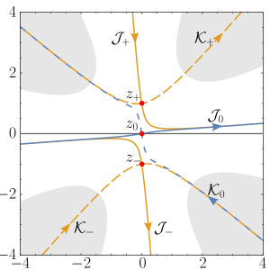
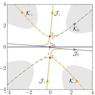
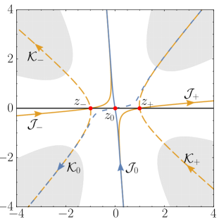
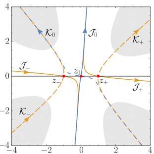
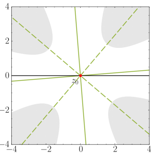
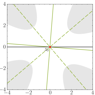
Figure 1: Downward and upward flows associated to the functions $f(z,1)$ (upper panels), $f(z,-1)$ (middle panels) and $f(z,0)$ (lower panels) in the $z$ plane. The grey sectors correspond to the asymtptotic regions where the integral diverges. The red points are the saddles of the functions $f(z,m)$. Continuous and dashed lines denote downward and upward flows, respectively. The lower panels correspond to the degenerate case, where multiple downward and upward flows depart from a saddle point. We have taken ${\rm Re}\,\lambda=1$, ${\rm Im}\,\lambda>0$ (left panels) and ${\rm Im}\,\lambda<0$ (right panels).

Consider first the case with $m>0$, which, as we will see, is not on a Stokes line for $\lambda$ real and positive. The function $f(z,m)$ has three saddle points: $z_{0}=0$, $z_{\pm}=\pm i\sqrt{m}$. For real $\lambda$ the upward flows from the saddle $z_{0}$ hit the two saddles $z_{\pm}$. This can be avoided by giving a small imaginary part to $\lambda$ as is shown in fig. 1 (first row) for positive (left) and negative (right) values of Im $\lambda$. The white regions are those where the integral is asymptotically convergent; by definition, the thimbles (continuous curves) start and end in these regions. The upward flows (dashed curves) instead start and end in the grey regions where the integrand diverges. Notice that the intersection numbers of the upward flows ${\cal K}_{\sigma}$ with the integration contour are the same in the two cases Im$\lambda\lessgtr 0$ ($n_{0}=1$, $n_{\pm}=0$). Therefore, the decomposition (2.5) is not ambiguous, ${\cal C}_{x}$ coincides with a single thimble and we are not on a Stokes line.

When $m<0$ the integral is on a Stokes line for real positive $\lambda$, since the saddle points are all on the real axis ($z_{0}=0$, $z_{\pm}=\pm\sqrt{-m}$). As before the upward flows from $z_{0}$ hit the other two saddles $z_{\pm}$, but now the intersection numbers jump across Im $\lambda=0$ ($n_{0}=\pm 1$, $n_{\pm}=1$), as can be seen in fig. 1 (second row). Depending on the sign of Im $\lambda$ the decomposition (2.5) reads

$$\begin{split}{\cal C}_{+}&={\cal J}_{-}-{\cal J}_{0}+{\cal J}_{+}\,,\qquad{\rm Im}~{}\lambda>0\,,\\ {\cal C}_{-}&={\cal J}_{-}+{\cal J}_{0}+{\cal J}_{+}\,,\qquad{\rm Im}~{}\lambda<0\,.\end{split}$$ (2.12)

The integrals over the two paths ${\cal C}_{\pm}$ coincide when Im $\lambda\to 0$, as manifest from the figure.

For $m=0$ the only saddle point at $z_{0}=0$ is degenerate (i.e. $f^{\prime\prime}(0)=0$) and multiple upward and downward flows depart from $z_{0}$ as illustrated in fig. 1 (third row). The decomposition rules (2.5) do not apply and analytic continuation of the parameter $\lambda$ does not help. One possible way to use saddle point techniques is to define the case $m=0$ as the limit $m\to 0$ of the previous cases, where the three saddle points $z_{0,\pm}$ collide. An alternative way will be described in sec. 2.4.

2.2 Asymptotic Series and Borel Sums

The integrals $Z_{\sigma}(\lambda)$ in eq. (2.9) can be evaluated using saddle-point expansions, that give generically rise to divergent asymptotic expansions. This is due to the fact that $\lambda=0$ is a singular point, since for any $\lambda<0$ the integral is divergent.

A series expansion associated to a function $Z(\lambda)$ is asymptotic if, for any fixed order $N$,

$$Z(\lambda)-\sum_{n=0}^{N}Z_{n}\lambda^{n}={\cal O}(\lambda^{N+1})\,,\quad{\rm as}\quad\lambda\rightarrow 0\,.$$ (2.13)

Different functions can have the same asymptotic expansion, for instance when the difference is suppressed by a factor $e^{-\alpha/\lambda}$, and hence the coefficients of the asymptotic series alone do not uniquely fix the function $Z(\lambda)$.

Divergent asymptotic series provide at best an approximate description of the function $Z(\lambda)$, with an accuracy that depends on the behaviour of the series coefficients $Z_{n}$ for $n\gg 1$. Suppose that for $n\gg 1$

$$Z_{n}\sim n!a^{n}n^{c}\,,$$ (2.14)

for some real parameters $a$ and $c$. The best accuracy for $Z(\lambda)$ is obtained by finding the value $N=N_{{\rm Best}}$ that minimizes the error $\Delta_{Z}\sim Z_{N}\lambda^{N}$. Using Stirling formula, one has

$$N_{{\rm Best}}\approx\frac{1}{|a|\lambda}\,,$$ (2.15)

where the error is asymptotically given by

$$\Delta_{Z}\sim e^{-\frac{1}{|a|\lambda}}\,,$$ (2.16)

independently of $c$ at leading order. This error is consistent with the intrinsic ambiguity related to asymptotic series discussed above. Keeping more than $N_{{\rm Best}}$ terms in the asymptotic series would lead to an increase in the error.

A possible way to reconstruct a function $Z(\lambda)$ with asymptotic expansion of the form

$$\sum_{n=0}^{\infty}Z_{n}\lambda^{n}$$ (2.17)

is via Borel resummation. We define the Borel transform

$${\cal B}Z(t)=\sum_{n=0}^{\infty}\frac{Z_{n}}{n!}t^{n}\,,$$ (2.18)

which is the analytic continuation of a series with non-zero radius of convergence. In the absence of singularities for $t>0$ the integral

$$Z_{B}(\lambda)=\int_{0}^{\infty}dt\,e^{-t}{\cal B}Z(t\lambda)$$ (2.19)

defines a function of $\lambda$ with the same asymptotic expansion as $Z(\lambda)$ and the series (2.17) is said to be Borel resummable. Since, as we mentioned, different functions can admit the same asymptotic series, certain properties of $Z(\lambda)$ and its behaviour near the origin have to be assumed to prove that $Z_{B}(\lambda)=Z(\lambda)$. These requirements are generically hard to verify. On the other hand, in the specific cases where $Z(\lambda)$ is defined as an integral, one might be able to rewrite it directly in the form (2.19), so that the equality $Z_{B}(\lambda)=Z(\lambda)$ can be proved without the need of verifying the above assumptions. This is the approach taken in this paper, as we will show in subsec. 2.3 and in sec. 3. When $Z_{B}(\lambda)=Z(\lambda)$ we say that the series (2.17) is Borel resummable to the exact result.

In the following we will be using a generalization of the Borel transform, due to Le Roy, obtained by defining

$${\cal B}_{b}Z(\lambda)\equiv\sum_{n=0}^{\infty}\frac{Z_{n}}{\Gamma(n+1+b)}\lambda^{n}\,,$$ (2.20)

where $b$ is an arbitrary real parameter. The function $Z_{B}(\lambda)$ now reads

$$Z_{B}(\lambda)=\int_{0}^{\infty}\!dt\,t^{b}e^{-t}\,{\cal B}_{b}Z(\lambda t)\,,$$ (2.21)

and clearly ${\cal B}_{0}Z(t)={\cal B}Z(t)$. Borel-Le Roy trasforms with different $b$ can be related analytically as follows:

$$\begin{split}{\cal B}_{b}(t)&=t^{-b}\partial_{t}^{n}\left[t^{b+n}{\cal B}_{b+n}(t)\right]\,,\qquad n\in\mathbb{N}^{+}\\ {\cal B}_{b+\alpha}(t)&=\frac{t^{-b-\alpha}}{\Gamma(\alpha)}\int_{0}^{t}dt^{\prime}\,\frac{(t^{\prime})^{b}\,{\cal B}_{b}(t^{\prime})}{(t-t^{\prime})^{1-\alpha}}\,,\qquad 0<\alpha<1\,.\end{split}$$ (2.22)

Note that the position of the singularities of two Borel-Le Roy transforms is the same, which implies that Borel summability does not depend on $b$, though the nature of the singularities might.

The analytic structure of the Borel transform is connected to the large order behaviour of the asymptotic series. For example the coefficient $a$ in eq. (2.14) determines the position of the singularity closest to the origin ($\lambda t_{\star}=1/a$). If $a<0$ the series alternates in sign, the singularity is on the negative real axis of $t$ and the series is Borel resummable in the absence of further singularities on the positive real axis. For $a>0$ the closest singularity is on the real axis and the series is not Borel resummable. In this case a lateral Borel resummation can be defined by slightly deforming the integration contour of eq. (2.19) above or below the singularity. The resulting ambiguity in the choice of the path is of order $e^{-t_{\star}}=e^{-1/(a\lambda)}$, i.e. ${\cal O}(\Delta_{Z})$. This ambiguity signals the presence of extra non-perturbative contributions to $Z(\lambda)$ not captured by $Z_{B}(\lambda)$. A systematic way of reconstructing the non-perturbative effects from the perturbative series is the subject of resurgence [6]. As we will discuss in detail in the following, for functions $Z(\lambda)$ of the form (2.1) the deformation defining the lateral Borel resummation corresponds to the one needed to avoid Stokes lines in the geometric description of subsec. 2.1. This leads to non-vanishing intersection numbers (2.6). For path integrals these numbers are generically infinite but, luckily enough, we will not need to compute them (neither algebraically through resurgence nor geometrically through Picard-Lefschetz theory), as we will show in the next two subsections. This is in fact one of the central results of this paper.

2.3 Borel Summability of Thimbles

We saw in subsec. 2.1 that the integral $Z(\lambda)$ can be decomposed into a sum of integrals over thimbles $Z_{\sigma}(\lambda)$. We will show now that each of these integrals admits an asymptotic expansion which is Borel resummable to the exact result.

Consider the following change of variable [24, 25]:

$$t=\frac{f(z)-f(z_{\sigma})}{\lambda}\,.$$ (2.23)

Recalling eq. (2.4), we see that for any value of $z$ along ${\cal J}_{\sigma}$ the variable $t$ is real and non-negative. For each value of $t\neq 0$, there are two values $z_{1,2}(\lambda t)\in{\cal J}_{\sigma}$ satisfying eq. (2.23): one for each of the two branches of the downward flow. We take $z_{1}$ and $z_{2}$ to be along and opposite to the direction of the thimble. After this change of variable we get

$$Z_{\sigma}(\lambda)=e^{-f(z_{\sigma})/\lambda}\,\int_{0}^{\infty}dt\,t^{-1/2}\,e^{-t}B_{\sigma}(\lambda t)\,,\quad B_{\sigma}(\lambda t)\equiv\sqrt{\lambda t}\bigg{(}\frac{g(z_{1}(\lambda t))}{f^{\prime}(z_{1}(\lambda t))}-\frac{g(z_{2}(\lambda t))}{f^{\prime}(z_{2}(\lambda t))}\bigg{)}\,.$$ (2.24)

For small $t$’s, we can expand $f(z)-f(z_{\sigma})\propto z^{2}$ (recall that $f^{\prime\prime}(z_{\sigma})\neq 0$) giving $f^{\prime}(z_{1,2}(t))\propto\sqrt{t}$ so that $B_{\sigma}(\lambda t)$ is analytic in the origin. The reader may recognize eq. (2.24) as the Laplace trasform of the Borel-Le Roy resummation formula (2.21) with

$$B_{\sigma}(\lambda t)={\cal B}_{-1/2}Z_{\sigma}(\lambda t)\,.$$ (2.25)

In particular the coefficients of the expansion of $B_{\sigma}(\lambda)$ around the origin are related to those of $Z_{\sigma}(\lambda)$ by $B_{\sigma}^{(n)}=Z_{\sigma}^{(n)}\Gamma(n+1/2)$. The function $B_{\sigma}(\lambda t)$ is analytic on the whole semipositive real $t$ axis given the regularity of $f(z)$ and $g(z)$ and the absence of other saddle points for $f(z)$ along the thimble. This proves that the power series of $Z_{\sigma}(\lambda)$ is Borel resummable. Not only, but having been able to rewrite the integral directly in terms of a Borel transform of the associated asymptotic expansion, we are guaranteed that the Borel resummation reproduces the full function $Z_{\sigma}(\lambda)$.

The original integral (2.1) can then be computed using eq. (2.8) and Borel resummation of the perturbative expansion of the $Z_{\sigma}$’s given in eq. (2.24). The contribution associated to the trivial saddle (i.e. the one with the smallest $f(z_{\sigma})$) can be seen as the perturbative contribution to $Z(\lambda)$, while the other saddles can be interpreted as non-perturbative effects. When only one saddle contributes, the perturbative contribution is Borel resummable to the exact result. When more saddles contribute, the perturbative expansion, although Borel resummable, does not reproduce the full result. If $Z(\lambda)$ is on a Stokes line some of the perturbative expansions of the thimbles are not Borel resummable. This is due to singularities of the Borel function induced by the presence of other saddles in the steepest descent path ($f^{\prime}(z_{1,2}(\lambda t))=0$ for $z\neq z_{\sigma}$).

We illustrate the results above using the explicit examples of eq. (2.10). We start with the case $m>0$ and, without loss of generality, set $m=1$. The original integration path coincides with the thimble ${\cal J}_{0}$, the only one that contributes, and the perturbative expansion is expected to be Borel resummable to the exact result. The coefficients $Z^{(m=1)}_{\sigma=0,n}$ of the perturbative expansion of $Z(\lambda,1)$ read

$$Z_{0,n}^{(1)}=\sqrt{2}(-)^{n}\frac{\Gamma(2n+\frac{1}{2})}{n!}\,.$$ (2.26)

For large $n$ we have

$$Z_{0,n}^{(1)}=(-4)^{n}\frac{\Gamma(n)}{\sqrt{\pi}}\left(1+{\cal O}\Big{(}\frac{1}{n}\Big{)}\right).$$ (2.27)

The Borel-Le Roy transform (2.20) with $b=-1/2$ gives

$${\cal B}_{-1/2}Z_{0}^{(1)}(\lambda t)=\sqrt{\frac{1+\sqrt{1+4\lambda t}}{1+4\lambda t}}\,,$$ (2.28)

which presents a branch-cut singularity in the $t$-plane at $\lambda t_{\star}=-1/4$ but it is regular on the positive real axis. By integrating over $t$ one reproduces the exact result (2.11):

$$\int_{0}^{\infty}\!dt\,t^{-\frac{1}{2}}e^{-t}{\cal B}_{-1/2}Z_{0}^{(1)}(\lambda t)=\frac{1}{\sqrt{2\lambda}}e^{\frac{1}{8\lambda}}K_{\frac{1}{4}}\Big{(}\frac{1}{8\lambda}\Big{)}=Z(\lambda,1)\,.$$ (2.29)

In this simple case we can also explicitly solve for the change of variable (2.23):

$$z_{1,2}(\lambda t)=\pm\sqrt{\sqrt{1+4\lambda t}-1}\,,$$ (2.30)

and check the validity of eq. (2.25). The form of ${\cal B}_{b}Z^{(1)}_{0}$ depends on the value of $b$. For instance, the standard Borel function ${\cal B}_{0}Z^{(1)}_{0}$ associated to eq. (2.26) equals

$${\cal B}_{0}Z^{(1)}_{0}(\lambda t)=\sqrt{\frac{8}{\pi}}\frac{K\Big{(}\frac{-1+\sqrt{1+4\lambda t}}{2\sqrt{1+4\lambda t}}\Big{)}}{(1+4\lambda t)^{1/4}}\,,$$ (2.31)

where $K(x)$ is the complete elliptic integral of the first kind. One can check that eq. (2.31) is in agreement with eq. (2.28) using the formula (2.22). We also see, as mentioned, that the position of the singularity of ${\cal B}_{0}Z^{(1)}_{0}$ and ${\cal B}_{-1/2}Z^{(1)}_{0}$ is the same.

The integral with $m<0$ is more interesting because $Z(\lambda,m)$ has a non-trivial thimble decomposition and is on a Stokes line. As we discussed, this is avoided by taking complex values of $\lambda$. Depending on the sign of Im $\lambda$ the two distinct decompositions in eq. (2.12) are generated. Setting $m=-1$ for simplicity and factoring out $e^{-f(z_{\sigma})/\lambda}$ from each $Z^{(m=-1)}_{\sigma}(\lambda)$, the coefficients of the perturbative expansions read

$$Z^{(-1)}_{\pm,n}=\frac{\Gamma\left(2n+\frac{1}{2}\right)}{n!}\,,\qquad Z^{(-1)}_{0,n}=iZ^{(1)}_{0,n}\,\,.$$ (2.32)

The Borel-Le Roy transform (2.20) with $b=-1/2$ gives

$${\cal B}_{-1/2}Z_{\pm}^{(-1)}(\lambda t)=\sqrt{\frac{1+\sqrt{1-4\lambda t}}{2(1-4\lambda t)}}\,,\;\;\quad{\cal B}_{-1/2}Z_{0}^{(-1)}(\lambda t)=i{\cal B}_{-1/2}Z_{0}^{(1)}(\lambda t)\,.$$ (2.33)

The Borel-Le Roy functions ${\cal B}_{-1/2}Z_{\pm}^{(-1)}$ have a branch-cut singularity in the $t$-plane at $t=1/(4\lambda)$ and for real positive $\lambda$ the asymptotic series with coefficients $Z^{(-1)}_{\pm,n}$ are not Borel resummable. However, the small imaginary part in $\lambda$ needed to avoid the Stokes lines would also allow us to avoid the singularity that now moves slightly below or above the real $t$ axis for Im $\lambda$ respectively positive or negative. We are effectively performing a lateral Borel summation. After integrating over $t$ we get

$$\begin{split}Z^{(-1)}_{\pm}(\lambda)&={\rm sign(Im}\lambda)\,\frac{ie^{\frac{1}{8\lambda}}}{2\sqrt{\lambda}}K_{\frac{1}{4}}\Big{(}-\frac{1}{8\lambda}\Big{)}\,,\\ Z^{(-1)}_{0}(\lambda)&=iZ_{0}^{(1)}(\lambda)\,.\end{split}$$ (2.34)

Using eq.(2.12), the sum of the three contributions in the limit Im $\lambda\to 0$ gives

$$\sqrt{\frac{\pi^{2}}{4\lambda}}e^{\frac{1}{8\lambda}}\left[I_{-\frac{1}{4}}\left(\frac{1}{8\lambda}\right)+I_{\frac{1}{4}}\left(\frac{1}{8\lambda}\right)\right]=Z(\lambda,-1)\,.$$ (2.35)

Notice that the discontinuity of the intersection number $n_{0}=-{\rm sign(Im}\lambda)$ as Im$\lambda\rightarrow 0$ fixes the ambiguity in the lateral Borel resummation of the perturbative series around the saddles $z_{\pm}$.

2.4 Exact Perturbation Theory

We have seen in the previous subsections how integrals of the form (2.1) can exactly be computed combining properly resummed saddle-point contributions. In particular, for real functions $f$, eq. (2.5) is trivial or not depending on the number of real saddles of $f$. We will explain in this subsection that the decomposition (2.5) in terms of thimbles can be modified. This implies that even when $f$ has more real saddles we can trivialize eq. (2.5) so that $Z(\lambda)$ is reproduced by a saddle-point expansion around one (perturbative) saddle only. This observation will play a crucial role when considering QM, since the computation of the intersection numbers (2.6) is far from trivial in the path integral case.

The Lefschetz thimble decomposition associated to the integral (2.1) is governed by the saddle points of $f$ and in particular it is independent of the prefactor $g(x)$. Define the function

$$\hat{Z}(\lambda,\lambda_{0})\equiv\frac{1}{\sqrt{\lambda}}\int_{-\infty}^{\infty}\!\!dx\,e^{-\hat{f}(x)/\lambda}\hat{g}(x,\lambda_{0})\,,$$ (2.36)

where

$$\hat{f}(x)\equiv f(x)+\delta f(x)\,,\quad\quad\hat{g}(x,\lambda_{0})\equiv g(x)e^{\delta f(x)/\lambda_{0}}\,,$$ (2.37)

are regular functions of $x$ that satisfy the same conditions as $f(x)$ and $g(x)$, in particular $\lim_{|x|\to\infty}\delta f(x)/f(x)=0$. The original integral is recovered by setting $\lambda_{0}=\lambda$:

$$\hat{Z}(\lambda,\lambda)=Z(\lambda)\,.$$ (2.38)

From the point of view of the saddle-point expansion in $\lambda$ at fixed $\lambda_{0}$, the function $\delta f$ inside $\hat{f}$ is a “classical” modification of $f$, while the factor of $\delta f$ in $\hat{g}$ is a “quantum” deformation. At fixed $\lambda_{0}$, the thimble decomposition of the integral (2.36) is determined by the downward and upward flows associated to the saddle points $z_{\hat{\sigma}}$ of $\hat{f}$ and not to the original saddles $z_{\sigma}$ of $f$. By properly choosing the function $\delta f$, we can generally construct a function $\hat{f}$ with only one real saddle $x_{0}$ (for convenience chosen such that $\hat{f}(x_{0})=0$) that trivializes the thimble decomposition to ${\cal C}={\cal C}_{x}$. While $Z(\lambda)$ may lie on a Stokes line, so that its perturbation theory is non-Borel resummable and requires extra non-perturbative contributions, the asymptotic expansion of $\hat{Z}(\lambda,\lambda_{0})$ in $\lambda$ at fixed $\lambda_{0}$ will be Borel-resummable to the exact result $\hat{Z}(\lambda,\lambda_{0})$. Setting then $\lambda=\lambda_{0}$ allows us to derive the original function $Z(\lambda_{0})$.

We call the series expansion of $\hat{Z}(\lambda,\lambda_{0})$ in $\lambda$ at fixed $\lambda_{0}$ “exact perturbation theory” (EPT), while we call the ordinary expansion of $Z(\lambda)$ “standard perturbation theory” (SPT). Note that in general SPT includes both perturbative and non-perturbative saddles.

We illustrate the method by reconsidering the example (2.11) with $m=-1$, where the contour decomposition (2.12) required three different saddle-point contributions. Consider the choice

$$\delta f(x)=x^{2}\,,$$ (2.39)

so that

$$\hat{f}(x)=\frac{1}{2}x^{2}+\frac{1}{4}x^{4}=f(x,1)\,,\quad\quad\hat{g}(x,\lambda_{0})=\exp\Big{(}\frac{x^{2}}{\lambda_{0}}\Big{)}\,.$$ (2.40)

The thimble decomposition is now determined by $f(x,1)$, in which case we know that ${\cal C}_{x}$ coincides with a thimble. The coefficients of the corresponding perturbative expansion read

$$\hat{Z}_{n}(\lambda_{0})=\sqrt{2}(-)^{n}\frac{\Gamma(2n+\frac{1}{2})}{n!}{}_{1}F_{1}\Big{(}-n,\frac{1}{2}-2n;-\frac{2}{\lambda_{0}}\Big{)}\,,$$ (2.41)

where ${}_{1}F_{1}(a,b;z)$ is the Kummer confluent hypergeometric function. At any fixed $\lambda_{0}$, the Kummer function for $n\gg 1/\lambda_{0}^{2}$ asymptotes to $\exp(-1/\lambda_{0})$ and for large $n$ we have

$$\hat{Z}_{n}(\lambda_{0})\approx e^{-\frac{1}{\lambda_{0}}}(-4)^{n}\frac{\Gamma(n)}{\sqrt{\pi}}\left(1+{\cal O}\Big{(}\frac{1}{n}\Big{)}\right)\,,$$ (2.42)

where the size of the ${\cal O}(1/n)$ subleading terms depends on $\lambda_{0}$. The Borel resummation of the perturbative series gives

$${\cal B}_{-1/2}\hat{Z}(\lambda t,\lambda_{0})=\sum_{n=0}^{\infty}\frac{\hat{Z}_{n}(\lambda_{0})}{\Gamma(n+1/2)}(\lambda t)^{n}\,.$$ (2.43)

Recovering the formula for the Borel transform from this equation is non-trivial. We can however use eq. (2.24) to get

$${\cal B}_{-1/2}\hat{Z}(\lambda t,\lambda_{0})={\cal B}_{-1/2}Z^{(1)}_{0}(\lambda t)\ e^{\frac{\sqrt{1+4\lambda t}-1}{\lambda_{0}}}\,,$$ (2.44)

where ${\cal B}_{-1/2}Z^{(1)}_{0}$ is the Borel-Le Roy function associated to the $m=1$ case, given in eq. (2.28). As expected, no singularities are present on the positive real $t$ axis. By taking $\lambda_{0}=\lambda$ and performing the integral over $t$ one reproduces the exact result for $Z(\lambda,-1)$ given in eq. (2.11):

$$\hat{Z}(\lambda,\lambda)=\int_{0}^{\infty}\!dt\,t^{-\frac{1}{2}}e^{-t}{\cal B}_{-1/2}\hat{Z}(\lambda t,\lambda)=Z(\lambda,-1)\,.$$ (2.45)

The above considerations are easily extended to more general functions $f(x)$. In particular, for polynomial functions of degree $2n$, independently of the location of the $2n-1$ saddle points and of the corresponding thimble decomposition associated to $f(z)$, we can always construct a function $\hat{f}(z)$, for example $\hat{f}(z)=z^{2}+f^{(2n)}(0)z^{2n}/(2n)!$, which has only one real saddle point and a trivial thimble decomposition. Notice that the choice of allowed $\delta f(x)$ is arbitrary and all of them are equally good.

Interestingly enough, the method above provides also an efficient way to study degenerate cases with $f^{\prime\prime}(z_{\sigma})=0$, where perturbation theory is ill-defined. Instead of deforming the function $f(z)$, e.g. by adding a small quadratic term $\epsilon z^{2}$, and of analyzing the integral in the limit $\epsilon\rightarrow 0$, we can more simply consider an appropriate function $\delta f(z)$ that removes the degeneracy, bypassing the need of taking a limit. For example, consider the integral (2.11) at $m=0$ with the choice

$$\delta f(x)=\frac{x^{2}}{2}\,,$$ (2.46)

so that

$$\hat{f}(x)=\frac{1}{2}x^{2}+\frac{1}{4}x^{4}=f(x,1)\,,\qquad\hat{g}(x,\lambda_{0})=e^{\frac{x^{2}}{2\lambda_{0}}}\,.$$ (2.47)

Since this case corresponds to the previous one with $m=-1$ via the rescaling $\lambda_{0}\to 2\lambda_{0}$, the Borel resummation of the perturbative expansion is simply given by ${\cal B}_{-1/2}\hat{Z}(\lambda t,2\lambda_{0})$, with ${\cal B}_{-1/2}\hat{Z}$ given in eq. (2.44). Taking $\lambda_{0}=\lambda$ and performing the integral over $t$, one reproduces the exact result

$$\int_{0}^{\infty}\!dt\,t^{-\frac{1}{2}}e^{-t}{\cal B}_{-1/2}\hat{Z}(\lambda t,2\lambda)=\frac{\Gamma\left(1/4\right)}{\sqrt{2}}\,\lambda^{-1/4}\,.$$ (2.48)

2.5 The Asymptotic Behaviour from Semiclassics

The saddle-points, whether or not they contribute to the integral (2.1), dictate the large-order behaviour of the series expansion of adjacent saddles. In QM this method has been first used by Bender and Wu in ref.[23] and extended to QFT by Lipatov [10] (see also refs.[11, 12, 13] for early extensive studies). For the specific case of finite-dimensional integrals a more rigorous derivation can be found in refs.[24, 25], where an exact resurgent formula relating the asymptotic series of different saddles has been derived. It has been shown in ref.[24] that the leading large order behaviour of the coefficients $Z_{\sigma,n}$ is governed by other saddles close to $z_{\sigma}$. More precisely, consider the integral (2.9) as a function of $\lambda=|\lambda|\exp(i\theta)$. The thimble ${\cal J}_{\sigma}(\theta)$ moves in the complex $z$-plane as $\theta$ is varied. For the special values of $\theta$ where the thimble crosses other saddle points the integral is on a Stokes line. These saddles are called “adjacent” to $z_{\sigma}$. Among the adjacent saddles, we denote by $z_{\sigma_{0}}$ the leading adjacent saddle as the one with the smallest value of $|f(z_{\sigma_{0}})-f(z_{\sigma})|$. Modulo an overall phase, the large-order behaviour of $Z_{\sigma,n}$ is given by the lowest-order coefficient $Z_{\sigma_{0},0}$ of the series associated to the leading adjacent saddle $z_{\sigma_{0}}$ [24]:

$$Z_{\sigma,n}=\sum_{{z_{\sigma_{0}}}}Z_{\sigma_{0},0}\frac{(n-1)!}{(f(z_{\sigma_{0}})-f(z_{\sigma}))^{n}}\left(1+{\cal O}\Big{(}\frac{1}{n}\Big{)}\right)\,,$$ (2.49)

where $Z_{\sigma_{0},0}=g(z_{\sigma_{0}})/\sqrt{2\pi|f^{\prime\prime}(z_{\sigma_{0}})|}$ and the sum is present in case we have more than one saddle with the same minimal value of $|f(z_{\sigma_{0}})-f(z_{\sigma})|$. Equation (2.49) justifies and generalizes our working assumption (2.14) which was valid only for real values of $f(z_{\sigma_{0}})-f(z_{\sigma})$. Matching the two equations we get

$$a=\frac{1}{f(z_{\sigma_{0}})-f(z_{\sigma})}\,,\quad\quad c=-1\,.$$ (2.50)

As we mentioned, the coefficient $a$ dictates the location of the leading singularities (i.e. the ones closest to the origin) of the Borel function ${\cal B}Z(t)$. For real functions $f$ with more than one saddle on the real axis the expansion around a minimum $z_{\sigma}$ gives $a$ real and positive, in agreement with the non-Borel summability of an asymptotic expansion on a Stokes line. It is clear from eq. (2.49) that in general the Borel function can have leading singularities for complex values of its argument, as anticipated in footnote 9.

The $n$-dependence of the leading large-order behaviour is governed by the function $f(z)$ and is independent of $g(z)$, the latter entering only in the determination of the overall normalization of the coefficients. For EPT this implies that at fixed $\lambda_{0}$, the $n$-dependence of the leading large order behavior of $\hat{Z}_{n}(\lambda_{0})$ does not depend on $\lambda_{0}$. More precisely we have, using eq. (2.49),

$$\hat{Z}_{n}(\lambda_{0})\approx\sum_{{z_{0}}}Z_{z_{0},0}\frac{(n-1)!}{(\hat{f}(z_{0})-\hat{f}(x_{0}))^{n}}\left(1+{\cal O}\left(\frac{1}{n}\right)\right)\,,\quad\quad Z_{z_{0},0}=e^{\frac{\delta f(z_{0})}{\lambda_{0}}}\frac{g(z_{0})}{\sqrt{2\pi|\hat{f}^{\prime\prime}(z_{0})|}}\,,$$ (2.51)

where $z_{0}$ are the leading adjacent saddles associated to the (unique) real saddle $x_{0}$ and $Z_{z_{0},0}$ is the leading order term of the series associated to $z_{0}$. Given the above choice of $\hat{f}(z)$, the factor $\hat{f}(z_{0})-\hat{f}(x_{0})$ in eq. (2.51) is always either complex or real negative, so that no singularities appear in the positive real $t$ axis of ${\cal B}\hat{Z}(t)$. Equation (2.51) is valid at fixed $\lambda_{0}$ for parametrically large values of $n$. More specifically we need $n\gg 1$ and $n\gg 1/\lambda_{0}^{2}$ in order to suppress the contributions coming from the higher-order coefficient terms $Z_{z_{0},1}$, $Z_{z_{0},2},\ldots$ associated to the leading adjacent saddle series $Z_{z_{0},n}$. The large-order behaviour (2.42) is immediately reproduced using eq. (2.51).

3 Path Integrals in QM

In this section, after having generalized the results of sec. 2 to higher dimensional integrals, we extend them to path integrals and introduce EPT in QM.

3.1 Higher Dimensional Integrals

The analysis of the one-dimensional integral (2.1) performed in sec. 2 can be extended to $n$-dimensions. Interpreting the domain of integration as an $n$-dimensional cycle ${\cal C}_{\bm{x}}={\mathbb{R}}^{n}$ in $n$ complex dimensions (with coordinates ${\bm{z}}$), like in eq. (2.2), downward and upward flows can be defined generalizing eq. (2.3). For each saddle ${\bm{z}}_{\sigma}$, the Lefschetz thimble ${\cal J}_{\sigma}$ and its dual cycle ${\cal K}_{\sigma}$ are obtained by taking the union of all the down- and up- ward flows. As for the 1-dimensional case possible Stokes lines can be avoided by taking $\lambda$ complex. After decomposing the cycle ${\cal C}_{\bm{x}}$ in terms of thimbles, like in eq. (2.5), we are left with the evaluation of integrals of the type

$$Z_{\sigma}(\lambda)=\lambda^{-n/2}\int_{{\cal J}_{\sigma}}d{\bm{z}}\,g({\bm{z}})\,e^{-f({\bm{z}})/\lambda}\,,$$ (3.1)

with $f$ and $g$ regular functions and such that the integral is convergent for any positive $\lambda$. By construction the function $f$ has only one non-degenerate saddle $\bm{z}_{\sigma}$: ${\bm{\nabla}}f({\bm{z}}_{\sigma})=0$ with $\det[\partial_{i}\partial_{j}f({\bm{z}_{\sigma}})]\neq 0$. Repeating the same steps as for the one-dimensional case and using known results from Morse theory, we can prove that the formal series expansion for $Z_{\sigma}(\lambda)$ around $\lambda=0$ is Borel resummable to the exact result. Indeed performing the change of variables

$$t=\frac{f({\bm{z}})-f({\bm{z}}_{\sigma})}{\lambda}\,,$$ (3.2)

we have (see also refs.[25, 26, 27])

$$\begin{split}Z_{\sigma}(\lambda)&=e^{-f(\bm{z}_{\sigma})/\lambda}\int_{0}^{\infty}dt\,t^{n/2-1}\,e^{-t}\,B_{\sigma}(\lambda t)\,,\\ B_{\sigma}(\lambda t)&\equiv(\lambda t)^{1-n/2}\int_{{\cal J}_{\sigma}}d\bm{z}\,g({\bm{z}})\,\delta[f(\bm{z})-f(\bm{z}_{\sigma})-\lambda t]\,.\end{split}$$ (3.3)

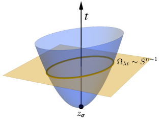
Figure 2: The support of integration $\Omega_{\lambda t}$ of the Borel function in $n$ dimensions with topology $S^{n-1}$ is the section of the thimble identified by the constraint (3.2).

The integral in $B_{\sigma}(\lambda t)$ has support over the $(n-1)$-dimensional hypersurface $\Omega_{\lambda t}$, defined by the constraint $f({\bm{z}})=f({\bm{z}}_{\sigma})+\lambda t$ (see fig. 2). In the neighborhood of the minimum ${\bm{z}}_{\sigma}$ the hypersurface $\Omega_{\lambda t}$ has the topology of a compact $n-1$ dimensional sphere $S^{n-1}$. Theorems from Morse theory (see e.g. ref. [28]) guarantee that this will continue to be true for any $t$ as long as no other critical point of $f({\bm{z}})$ is met, which is true for thimbles away from Stokes lines. Moreover, since $\bm{\nabla}f(\bm{z})\neq\bm{0}$ for $\bm{z}\neq\bm{z}_{\sigma}$, it follows that the integral defining $B_{\sigma}(\lambda t)$ is finite for any value of $t>0$. Similarly to the one-dimensional case, for $t\to 0$ one has $\bm{\nabla}f(\bm{z})={\cal O}(t^{1/2})$. Taking into account the $\lambda t$ dependence from the volume form we see that $B_{\sigma}(\lambda t)$ is analytic in the whole semipositive real axis including the origin. We conclude that the power series of $Z_{\sigma}(\lambda)$ in $\lambda$ is Borel resummable to the exact result and $B_{\sigma}(t)={\cal B}_{n/2-1}Z_{\sigma}(t)$. Depending on whether $n$ is even or odd, the first relation in eq. (2.22) allows us to rewrite Borel and $b=-1/2$ Borel-Le Roy transforms as simple derivatives of the formula above, namely

$$\begin{split}{\cal B}_{0}Z_{\sigma}(t)&=\partial_{t}^{k-1}\int_{{\cal J}_{\sigma}}\!d\bm{z}\,g({\bm{z}})\,\delta[f(\bm{z})-f(\bm{z}_{\sigma})-t]\,,\qquad n=2k\,,\\ {\cal B}_{-1/2}Z_{\sigma}(t)&=\sqrt{t}\,\partial_{t}^{k}\int_{{\cal J}_{\sigma}}\!d\bm{z}\,g({\bm{z}})\,\delta[f(\bm{z})-f(\bm{z}_{\sigma})-t]\,,\qquad n=2k+1\,.\end{split}$$ (3.4)

3.2 The Lefschetz Thimble Approach to the Path Integral

We are now ready to discuss path integrals in QM. Consider

$${\cal Z}(\lambda)=\int{\cal D}x(\tau)\,G[x(\tau)]e^{-S[x(\tau)]/\lambda}\,,$$ (3.5)

with $\tau$ the Euclidean time. The action $S$ is of the form

$$S[x]=\int d\tau\,\left[\frac{1}{2}\dot{x}^{2}+V(x)\right]\,,$$ (3.6)

where the potential $V(x)$ is assumed to be an analytic function of $x$, with $V(x)\to\infty$ for $|x|\to\infty$, so that the spectrum is discrete. In analogy to the finite dimensional cases the functionals $S[x]$ and $G[x]$ are regular and such that the path integral is well-defined for any $\lambda\geq 0$. The measure ${\cal D}x$ includes a $\lambda$-dependent normalization factor to make ${\cal Z}(\lambda)$ finite. The integration is taken over real $x(\tau)$ configurations satisfying the boundary conditions of the observable of interest.

By definition the path integral is the infinite dimensional limit of a finite dimensional integral, namely eq. (3.5) means

$${\cal Z}(\lambda)=\lim_{N\to\infty}\int{\cal D}^{(N)}x(\tau)\,G^{(N)}[x(\tau)]e^{-S^{(N)}[x(\tau)]/\lambda}\,,$$ (3.7)

where the limit is now explicit and $G^{(N)}[x(\tau)]$, $S^{(N)}[x(\tau)]$, ${\cal D}^{(N)}x(\tau)$, are discretized versions of the functionals $G$ and $S$ and of the path integral measure, which includes the factor $\lambda^{-N/2}$. Such limit can be twofold: The continuum limit, always present, and the infinite time limit, relevant for the extraction of certain observables. The former is not expected to generate problems in QM, since after having properly normalized the path integral all quantities are finite in this limit. The infinite time limit could instead be more subtle and we will discuss later when it may lead to troubles. For the moment we restrict our analysis to path integrals at finite time so that the limit in eq. (3.7) only refers to the continuum one.

Similarly to the finite dimensional case, the first step is to identify all the (real and complex) saddles $z_{\sigma}(\tau)$ (the solutions of the equations of motion) of the action $S[x]$ and to construct the analogue of the upward and downward flows from each $z_{\sigma}(\tau)$. Given the infinite dimensional nature of the path integral, the number of saddles is also infinite. In general a systematic analysis and computation of all the relevant flows and intersection numbers is impractical. In specific cases, however, only a few real saddle point solutions exist and we may hope to reconstruct the full answer from a finite set of saddle point expansions. In particular, if the equations of motion admit only one real solution, the domain of the integration (all real paths satisfying the boundary conditions) coincides with a thimble. We will now show that such path integral (and similarly any path integral over thimbles) admits a perturbation theory which is Borel resummable to the exact result.

The integral inside the limit in eq. (3.7) is finite dimensional and can now be treated as before, in particular we can rewrite it using eqs. (3.3) and (3.4) as

$$\begin{split}{\cal Z}(\lambda)&=\lim_{N\to\infty}e^{-\frac{S^{(N)}[x_{0}(\tau)]}{\lambda}}\int_{0}^{\infty}dt\,t^{-1/2}e^{-t}{\cal B}_{-1/2}^{(N)}{\cal Z}(\lambda t)\\ {\cal B}_{-1/2}^{(N)}{\cal Z}(\lambda t)&=\sqrt{\lambda t}\ \partial_{\lambda t}^{N}\int{\cal D}^{(N)}_{\lambda=1}x(\tau)\,G^{(N)}[x(\tau)]\,\delta[S^{(N)}[x(\tau)]-S^{(N)}[x_{0}(\tau)]-\lambda t]\,,\end{split}$$ (3.8)

where for definiteness we discretized the path integral into a $2N+1$ dimensional one and ${\cal D}_{\lambda=1}^{(N)}x(\tau)$ is the discretized measure without the $\lambda$ dependence (i.e. with $\lambda=1$). The regularity of the functionals $S$ and $G$ and the absence of other real saddle points allow a choice of discretization for which the Borel-Le Roy function ${\cal B}_{-1/2}^{(N)}{\cal Z}(\lambda t)$ is finite and integrable for any $N$. In QM the absence of divergences in the continuum limit strongly suggests that the exchange of the limit with the integral in the first line of eq. (3.8) can be performed safely. The function ${\cal B}_{-1/2}^{(\infty)}{\cal Z}(\lambda t)$ will then correspond to the Borel-Le Roy transform in the continuum limit, which will be integrable and will reproduce the full result ${\cal Z}(\lambda)$. As a check we verified the finiteness of ${\cal B}_{-1/2}^{(\infty)}{\cal Z}(\lambda t)$ at $\lambda t=0$ (which reproduces the known results for the harmonic oscillator) as well as at any order in $\lambda t$ in polynomial potentials (see the appendix).

We are then led to the following result:

If the action $S[x(\tau)]$ has only one real saddle point $x_{0}(\tau)$ satisfying the boundary conditions implicit in eq. (3.5), such that $\det S^{\prime\prime}[x_{0}(\tau)]\neq 0$, then no thimble decomposition is needed and the formal series expansion of ${\cal Z}(\lambda)$ around $\lambda=0$, corresponding to the saddle point expansion of the path integral, is Borel resummable to the exact result.

If the action $S[x]$ admits one real saddle only, in general it will admit several (or an infinite number of) complex saddles (or complex instantons). All these complex instantons, however, do not contribute to the path integral. Analogously to the finite-dimensional cases, whenever more than one real saddle point with finite action satisfying the boundary conditions of the path integral exists, the perturbative series generically will not be Borel resummable, as a result of the Stokes phenomenon.

Boundary conditions determine the number of real saddle points of $S$ and hence are of crucial importance to check the validity of our working assumption. As a result the same theory may have some observables that are Borel resummable to the exact result and some for which the perturbative series requires the inclusion of non-perturbative effects. It might be useful to illustrate the point with an example. Consider a QM system with an (inverted) potential like the one depicted in fig. 3 and define

$${\cal W}(\lambda,\beta,x_{0})=\int_{x(\beta/2)=x(-\beta/2)=x_{0}}{{\cal D}x(\tau)\,e^{-S[x(\tau)]/\lambda}}\ =\sum_{k}|\psi_{k}(x_{0};\lambda)|^{2}e^{-\beta E_{k}(\lambda)}\,,$$ (3.9)

where $E_{k}(\lambda)$ and $\psi_{k}(x;\lambda)$ are the eigenvalues and the eigenfunctions of the system, respectively. Depending on $x_{0}$, the action $S$ admits one or more real saddle points. For instance, for $x_{0}>x_{2}$ only one real solution exist. For $x_{0}<x_{2}$ depending on $\beta$ one or more real solutions are allowed.

The partition function is related to ${\cal W}(\lambda,\beta,x_{0})$ by

$${\cal Z}(\lambda,\beta)=\int_{-\infty}^{\infty}\!dx_{0}\,{\cal W}(\lambda,\beta,x_{0})=\sum_{n}e^{-\beta E_{n}(\lambda)}\,,$$ (3.10)

which corresponds to summing over all real periodic trajectories and it is not Borel resummable.

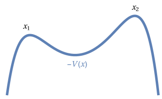
Figure 3: Sketch of a bounded (inverted) potential with more than one critical point.

We now discuss the infinite $\beta$ limit, which is relevant for the extraction of some observables such as the properties of the ground state (eigenvalue, eigenfunction, …). Unlike the continuum limit, the large-$\beta$ limit generically does not commute with the thimble decomposition. There are cases where the path integral admits more than one real saddle at finite $\beta$ but only one survives at $\beta\to\infty$. There are other cases instead where only one real saddle exists for any finite $\beta$ but the path integral lies on a Stokes line at $\beta=\infty$.

Consider for instance the ground state energy

$$E_{0}(\lambda)=-\lim_{\beta\rightarrow\infty}\frac{1}{\beta}\log{\cal Z}(\lambda,\beta)\,.$$ (3.11)

For the example of tilted double-well potential discussed before, ${\cal Z}(\lambda,\beta)$ has multiple real saddles for any finite $\beta$, corresponding to solutions of the equations of motion with period $\beta$. Besides the trivial one, $x(\tau)=x_{2}$, the leading saddle corresponds to the solution $x(\tau)=x_{1}$, which is suppressed by a factor $e^{-\beta[V(x_{1})-V(x_{2})]/\lambda}$. Therefore in the limit $\beta\to\infty$ only the thimble associated to the true minimum gives a non-vanishing contribution. The perturbative series for $E_{0}$ is then Borel resummable to the full answer, though ${\cal Z}(\lambda,\beta)$ at finite $\beta$ is not. This result is more manifest if we use the alternative formula

$$E_{0}(\lambda)=-\lim_{\beta\rightarrow\infty}\frac{1}{\beta}\log{\cal W}(\lambda,\beta,x_{2})\,.$$ (3.12)

Since ${\cal W}(\lambda,\beta,x_{2})$ has only one saddle ($x(\tau)=x_{2}$) for any $\beta$, the Borel summability of $E_{0}(\lambda)$ follows trivially from our analysis.

The same discussion applies for any bound-state potential with a unique global minimum. When the minimum is not unique generically the perturbative series of $E_{0}$ is not Borel resummable because in the large $\beta$ limit an infinite number of saddles with finite action are present, independently of the functional ${\cal W}$ used. This is also true if the degeneracy of the absolute minimum is lifted at the quantum level, i.e. $V(x_{1})-V(x_{2})={\cal O}(\lambda)$, as it will become more clear below. We will discuss in more detail the properties of the Borel transform of $E_{0}$ for the different cases in sec. 4.

The analysis is particularly simple for potentials $V(x)$ that have a single non-degenerate critical point (minimum). Without loss of generality we take it to be at the origin with $V(0)=0$. Indeed, independently of the boundary conditions, there is always a single real saddle point both at finite and infinite $\beta$. Since our considerations apply for any allowed choice of the functional $G[x]$ in eq. (3.5) we are led to argue that perturbative series of any observable is Borel resummable to the exact result. By any observable we mean any path integral with regular boundary conditions and analytic functions of them, such as partition functions, energy eigenvalues, eigenfunctions, etc. In this way we recover in a simple and intuitive way known results [2, 3, 29] on the Borel summability of the energy spectrum of a class of anharmonic potentials and extend them to more general QM systems and observables.

3.3 Exact Perturbation Theory

Interestingly enough, the method of subsec. 2.4 can easily be extended to the QM path integral (3.5). Suppose we can split the potential $V=V_{0}+\Delta V$ into the sum of two potentials $V_{0}$ and $\Delta V$ such that

1. $V_{0}$ has a single non-degenerate critical point (minimum);

2. $\lim_{|x|\rightarrow\infty}\Delta V/V_{0}=0$ .

Consider then the auxiliary potential

$$\hat{V}=V_{0}+\frac{\lambda}{\lambda_{0}}\Delta V\equiv V_{0}+\lambda V_{1}\,,$$ (3.13)

where $\lambda_{0}$ is an arbitrary positive constant and define the modified path integral

$$\hat{\cal Z}(\lambda,\lambda_{0})=\int{\cal D}x\ G[x]\ e^{-\frac{\int\!d\tau\,\Delta V}{\lambda_{0}}}\ e^{-\frac{S_{0}}{\lambda}}\,,\qquad S_{0}\equiv\int\!d\tau\left[\frac{1}{2}\dot{x}^{2}+V_{0}\right].$$ (3.14)

Since $\hat{\cal Z}(\lambda,\lambda)={\cal Z}(\lambda)$, the latter can be obtained by the asymptotic expansion in $\lambda$ of $\hat{\cal Z}$ (EPT), which is guaranteed to be Borel resummable to the exact answer.

We can then relax the requirement of a single critical point and state our general result:

All observables in a one-dimensional QM system with a bound-state potential $V$ for which points 1. and 2. above apply are expected to be entirely reconstructable from a single perturbative series.

Generally the decomposition $V=V_{0}+\Delta V$ is far from being unique. EPT is defined as an expansion around the minimum of $V_{0}$, which does not need to be a minimum (or a critical point) of the original potential $V$. The number of interaction terms present in EPT also depends on the particular decomposition performed and in general is higher than the number of interaction terms present in the original theory (SPT). Since the mass term we choose for $V_{0}$ might differ from the one of $V$, so will do the effective couplings of SPT and EPT. As long as conditions 1. and 2. above are fulfilled, any choice of EPT is equivalent to any other, though in numerical computations with truncated series some choices might be more convenient than others.

The leading large-order behaviour of the coefficients associated to the asymptotic expansion of the ground state energy associated to $\hat{\cal Z}(\lambda,\lambda_{0})$ can be deduced using the results of refs.[10, 11, 12] (see in particular sec. II of ref.[12]). The large-order behaviour of the ground state energy coefficients is governed by the action $S_{0}$ only. In analogy to the one-dimensional integral, the functional $G\exp(-\int\Delta V/\lambda_{0})$ in eq. (3.14) governs only the overall $n$-independent size of the coefficients.

Note that so far we used non-canonical variables with the coupling constant $\lambda$ playing the role of $\hbar$—the saddle-point expansion is the loopwise expansion. This means that in the canonical basis the potential $V(x)$ turns into $V(x;\lambda)$ defined as

$$V(x;\lambda)=\frac{V(\sqrt{\lambda}\,x)}{\lambda}\,.$$ (3.15)

On the other hand, the coupling constant dependence of a generic QM potential may not be of the form in eq. (3.15). For example, the expansion in $g$ for the potential

$$V(x;g)=x^{2}+gx^{4}+gx^{6}$$ (3.16)

does not correspond to the loopwise parameter. Indeed, setting $\lambda=\sqrt{g}$, the terms $x^{2}+\lambda^{2}x^{6}$ satisfy eq. (3.15) while the term $\lambda^{2}x^{4}$ is effectively a one-loop potential that should be included in the functional $G[x]$ of eq. (3.5).

4 Quantum Mechanical Examples

In this section we study numerically polynomial QM systems in SPT and EPT, providing extensive evidence of the results obtained in the previous sections. A summary of part of these results appeared in ref.[17].

The perturbative series in both SPT and EPT are obtained by using the Mathematica [30] package “BenderWu” of ref.[31] which is based on recursion relations among the perturbative coefficients first derived by Bender and Wu in refs.[32, 23]. We consider up to $N$ orders in the perturbative expansion (for EPT we fix the auxiliary parameter $\lambda_{0}$ to a given value) and we approximate the Borel function with Padé approximants. For definiteness we use the Borel-Le Roy function ${\cal B}_{b}{\cal Z}(\lambda)$ with $b=-1/2$, which numerically seems a convenient choice leading to more accurate Padé approximants. The numerical computation of the integral in eq. (2.21) gives the final result (evaluated for the value of the coupling $\lambda=\lambda_{0}$ in EPT). In the following we will refer to the above procedure as the Padé-Borel method. The result obtained is then compared with other numerical methods such as the Rayleigh-Ritz (RR) method (see e.g. ref.[33] for some explicit realizations). For polynomial potentials of small degree an efficient implementation is as follows: One starts from the truncated basis $|k_{0}\rangle$, $k=1,\ldots,N_{RR}$ of the harmonic oscillator eigenfunctions, and then computes the full Hamiltonian matrix $H_{kh}=\langle k_{0}|H|h_{0}\rangle$, which is almost diagonal. The approximate energy levels and eigenfunctions of the system are given by the eigenvalues and eigenvectors of $H_{kh}$. This method converges to the exact result very quickly. The accuracy depends on $N_{RR}$ and on the energy level considered. The lower is the level, the higher is the accuracy.

We mostly focus on the energy eigenvalues $E_{k}(\lambda)$, though the eigenfunctions $\phi_{k}(x;\lambda)$ are also considered. Since the package [31] computes non-normalized wavefunctions, we define

$$\psi_{k}(x;\lambda)\equiv\frac{\phi_{k}(x;\lambda)}{\phi_{k}(x_{0};\lambda)}$$ (4.1)

for some $x_{0}$ and compute

$$\Delta\psi_{k}(x;\lambda)=\frac{\psi_{k}^{\rm{RR}}(x;\lambda)-\psi_{k}^{\rm{EPT}}(x;\lambda)}{\psi_{k}^{\rm{RR}}(x;\lambda)}\,,$$ (4.2)

where for simplicity we omit the $x_{0}$ dependence in the $\psi_{k}(x;\lambda)$.

4.1 Tilted Anharmonic Oscillator

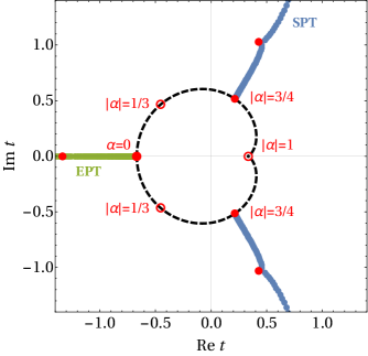
Figure 4: Location of the singularities in the Borel plane for the standard and exact perturbative series of $E_{0}(\lambda,\alpha)$ for the potential (4.3). The dashed line represents the location of the leading singularities as expected from eq. (4.4) with $|\alpha|\in[0,1]$. The red bullets indicate the position of the first and second complex instantons for $|\alpha|=3/4$. The regions where the simple poles of the Padé-Borel approximants accumulate are depicted in blue and green.

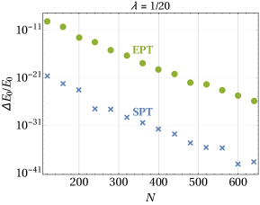
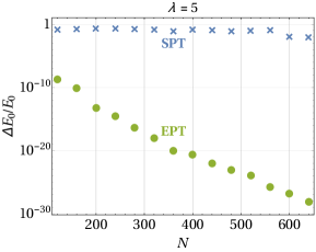
Figure 5: Comparison between the relative error $\Delta E_{0}/E_{0}$ in the computation of the ground state energy using Borel-Padé approximants of the series coming from eqs. (4.3) (SPT) and (4.5) (EPT) as a function of the number $N$ of series coefficients retained. (Left panel) weak coupling $\lambda=1/20$, (right panel) strong coupling $\lambda=5$.

The first example we consider is the tilted anharmonic oscillator

$$V(x;\lambda)=\frac{1}{2}x^{2}+\alpha\sqrt{\lambda}x^{3}+\frac{\lambda}{2}x^{4}\,,$$ (4.3)

where $\alpha$ is a real parameter. For $|\alpha|<2\sqrt{2}/3$, the potential has a unique minimum at $x=0$. According to our results, SPT is then Borel resummable to the exact value for all the observables. For $2\sqrt{2}/3\leq|\alpha|<1$ some quantities, such as the ground state energy $E_{0}(\lambda,\alpha)$, are Borel resummable to the exact value while some are not, such as the partition function. The cases $|\alpha|=1$ (symmetric double well) and $|\alpha|>1$ (false vacuum) will be discussed in the next subsections.

For definiteness, let us look at the ground state energy $E_{0}(\lambda,\alpha)$. The position of the leading singularities in the associated Borel plane is dictated by the value of the action $S[z_{\pm}]$ on the nearest saddle points, which for $|\alpha|<1$ are complex instantons $z_{\pm}$ [12]:

$$\lambda t_{\pm}=\lambda S[z_{\pm}]=-\frac{2}{3}+\alpha^{2}+\frac{1}{2}\alpha(\alpha^{2}-1)\Big{(}\log\frac{1-\alpha}{1+\alpha}\pm i\pi\Big{)}\,.$$ (4.4)

This expectation is confirmed by a numerical analysis with Borel-Padé approximants (see fig. 4). The ground state energy coefficients $E_{0,n}(\alpha)$ for $n\gg 1$ oscillate with a period given by $2\pi/|{\rm Arg}\,t_{\pm}|$. As long as the coefficients oscillate, the observable is Borel resummable. The period is minimum at $\alpha=0$, where the coefficients alternate, and grows with $|\alpha|$ until it becomes infinite at $|\alpha|=1$ and Borel resummability is lost. In numerical evaluations at fixed order $N$ the best accuracy is obtained at $\alpha=0$. For $\alpha\neq 0$, at least $N>2\pi/|{\rm Arg}\,t_{\pm}|$ orders are required to see the alternating nature of the series.

Even if $E_{0}(\lambda,\alpha)$ is Borel resummable for $|\alpha|<1$ in SPT, EPT can be used to greatly improve the numerical results at strong coupling. Indeed, we can define a potential $\hat{V}=V_{0}+\lambda V_{1}$ with

$$V_{0}=\frac{1}{2}x^{2}+\frac{\lambda}{2}x^{4}\,,\quad\quad V_{1}=\alpha\frac{\sqrt{\lambda}}{\lambda_{0}}x^{3}\,,$$ (4.5)

so that the original one is recovered for $\lambda_{0}=\lambda$.

The first terms in the perturbative SPT and EPT expansions read

$$E_{0} \!=\! \frac{1}{2}+\frac{3-11\alpha^{2}}{8}\lambda-\frac{21-342\alpha^{2}+465\alpha^{4}}{32}\lambda^{2}+\frac{333-11827\alpha^{2}+45507\alpha^{4}-39709\alpha^{6}}{128}\lambda^{3}+\ldots$$

$$\hat{E}_{0} \!=\! \frac{1}{2}+\frac{3}{8}\lambda-\frac{21}{32}\lambda^{2}+\Big{(}\frac{333}{128}-\frac{11\alpha^{2}}{8\lambda_{0}^{2}}\Big{)}\lambda^{3}+\ldots\,,$$ (4.6)

which shows how EPT rearranges all the $\alpha$-dependent terms in the perturbative expansion. For instance, the one-loop $\alpha^{2}$-dependent term in SPT appears at three loops in EPT.

As we discussed, $V_{1}$ modifies the overall normalization of the large-order coefficients $\hat{E}_{0,n}(\lambda_{0})$ with respect to the ones of the anharmonic oscillator $E_{0,n}(\alpha=0)$ without altering their leading large-order $n$-dependence. The normalization at leading order is given by the exponential of the integral of $V_{1}$ evaluated at the nearest complex saddles

$$\exp\Big{(}-\alpha\frac{\lambda^{3/2}}{\lambda_{0}}\int_{-\infty}^{\infty}\!d\tau\,z^{3}_{\pm}[\tau]\Big{)}=e^{\pm i\pi\alpha/2\lambda_{0}}\,.$$ (4.7)

In analogy to the one-dimensional case outlined at the end of sect. 2, we expect for $n\gg 1$ and $n\gg 1/\lambda_{0}^{2}$,

$$\hat{E}_{0,n}\Big{(}\frac{\lambda_{0}}{\alpha}\Big{)}=E_{0,n}(\alpha=0)\left[\cos\Big{(}\frac{\pi\alpha}{2\lambda_{0}}\Big{)}+{\cal O}\Big{(}\frac{1}{n}\Big{)}\right]\,,$$ (4.8)

where

$$E_{0,n}(\alpha=0)=-\frac{\sqrt{6}}{\pi^{3/2}}\left(-\frac{3}{2}\right)^{n}\Gamma\left(n+\frac{1}{2}\right)\left[1+{\cal O}\Big{(}\frac{1}{n}\Big{)}\right]\,.$$ (4.9)

In particular, eq. (4.8) implies that the leading singularity of the Borel function is located at $t=-2/3$ as in the case of the anharmonic oscillator with $\alpha=0$. This is numerically confirmed by the associated Borel-Padé approximants (see fig. 4). It is useful to compare the efficiency of SPT and EPT as a function of the number of terms $N$ that are kept in the series expansion. These are reported in fig.5 for weak and strong coupling values $\lambda=1/20$, $\lambda=5$, respectively, where $\Delta E_{0}$ refers to the discrepancy with respect to $E_{0}^{{\rm RR}}$.

In agreement with expectation, at sufficiently weak coupling SPT performs better than EPT. The situation is drastically different at strong coupling, where SPT is essentially inaccurate for any $N$ reported in fig.5, while EPT has an accuracy that increases with the order.

At fixed number of perturbative terms, EPT works at its best for coupling constants $\lambda\sim{\cal O}(1)$. Like SPT, as $\lambda$ increases the integral in eq. (2.21) is dominated by larger values of $t$ (this is best seen by rescaling $t\rightarrow t/\lambda$) and hence more and more terms of the perturbative expansion are needed to approximate the Borel function. On the other hand, in analogy to the one-dimensional case (2.44), the Borel function in EPT contains an additional exponential term coming from $\exp(-\int V_{1})$. When $\lambda\ll 1$ the accuracy drops because the coefficients $\hat{E}_{n}(\lambda_{0})$ are very large before reaching the regime when eq. (4.8) applies.

4.2 Symmetric Double-well

For $|\alpha|=1$ the potential (4.3) turns into a symmetric double-well, with two degenerate minima. This is the prototypical model where real instantons are known to occur and the perturbative expansion around any of the two minima are known to be not Borel resummable. SPT requires the addition of an infinite number of real instantons to fix the ambiguities related to lateral Borel resummations and to reproduce the full result, see e.g. ref.[36] for a numerical study.

$k$	$x=1/8$	$x=1/4$	$x=1/2$	$x=1$	$x=2$	$\Delta E_{n}/E_{n}$
Anharmonic
0	$7\cdot 10^{-24}$	$4\cdot 10^{-23}$	$2\cdot 10^{-22}$	$10^{-21}$	$8\cdot 10^{-20}$	$3\cdot 10^{-33}$
1	$3\cdot 10^{-15}$	$2\cdot 10^{-14}$	$7\cdot 10^{-14}$	$5\cdot 10^{-13}$	$3\cdot 10^{-11}$	$4\cdot 10^{-30}$
2	$2\cdot 10^{-8}$	$10^{-7}$	$4\cdot 10^{-6}$	$6\cdot 10^{-7}$	$7\cdot 10^{-6}$	$2\cdot 10^{-27}$
Symmetric double well
0	$5\cdot 10^{-27}$	$3\cdot 10^{-26}$	$10^{-25}$	$2\cdot 10^{-25}$	$3\cdot 10^{-24}$	$6\cdot 10^{-34}$
1	$4\cdot 10^{-18}$	$2\cdot 10^{-17}$	$10^{-16}$	$6\cdot 10^{-16}$	$2\cdot 10^{-14}$	$10^{-30}$
2	$5\cdot 10^{-11}$	$3\cdot 10^{-10}$	$3\cdot 10^{-9}$	$2\cdot 10^{-9}$	$10^{-8}$	$5\cdot 10^{-27}$

Table 1: Relative errors of the ratio of wave functions (4.2) and energies of the first three levels of the anharmonic and symmetric double well at $\lambda=1$, evaluated at different points $x$ using EPT with $N=200$, and RR methods. In the anharmonic case EPT coincides with SPT. We have taken $x_{0}=1/16$ in eq. (4.1).

Shifting the $x$ coordinate so that $x=0$ is the maximum of the potential

$$V(x;\lambda)=\frac{\lambda}{2}\left(x^{2}-\frac{1}{4\lambda}\right)^{2}\,,$$ (4.10)

we can perform an EPT by considering the auxiliary potential

$$V_{0}=\frac{1}{32\lambda}+\frac{\lambda_{0}}{2}x^{2}+\frac{\lambda}{2}x^{4}\,,\qquad V_{1}=-\Big{(}1+\frac{1}{2\lambda_{0}}\Big{)}\frac{x^{2}}{2}\,,$$ (4.11)

which has as effective couplings $\lambda/\lambda_{0}^{3/2}$ and $\lambda/\lambda_{0}(1+1/(2\lambda_{0}))$. This choice of EPT, where the minimum of $V_{0}$ is half way between the two minima of the double well, is such that the numerical Borel-Padé resummation is able to reconstruct the non-perturbative splitting between the first two levels at moderately small couplings, with a few hundred orders of perturbation theory. However, at fixed order $N$ of perturbation theory and for very small couplings, the true vacua depart further and further from the minimum of $V_{0}$ and the corresponding EPT becomes even worse than the naive truncated series. In this regime a better choice would be to take the minimum of $V_{0}$ close to one of the true minima of the double well (although resolving non-perturbative effects in this regime becomes harder and, as expected, more terms of the perturbative expansion are required).

We start by considering the ground state energy $E_{0}(\lambda)$. The large order behavior of the series coefficients $\hat{E}_{0,n}(\lambda_{0})$ in EPT for $n\gg 1$ and $n\gg 1/\lambda_{0}^{2}$ are given by

$$\hat{E}_{0,n}(\lambda_{0})=\lambda_{0}^{\frac{1}{2}-\frac{3}{2}n}\,e^{-\sqrt{\lambda_{0}}\big{(}1+\frac{1}{2\lambda_{0}}\big{)}}E_{0,n}(\alpha=0)\left[1+{\cal O}\Big{(}\frac{1}{n}\Big{)}\right]\,.$$ (4.12)

As before, the exponential $\lambda_{0}$-dependent factor is obtained by evaluating the potential $V_{1}$, the second term in square brackets in eq. (4.11), at the leading complex instanton solutions $z_{\pm}$. The prefactor $\lambda_{0}^{\frac{1}{2}-\frac{3}{2}n}$ is instead due to the $\lambda_{0}$ dependence of the quadratic term in $V_{0}$.

By taking $N=200,\lambda=\lambda_{0}=1/32$, we get $\Delta E_{0}/E_{0}\approx 2\cdot 10^{-5}$ and $\Delta E_{1}/E_{1}\approx 2\cdot 10^{-11}$. These accuracies are already several orders of magnitude smaller than the leading order one-instanton contribution

$$E_{0}^{\rm inst}\approx\frac{2}{\sqrt{\pi\lambda}}e^{-\frac{1}{6\lambda}}\,,$$ (4.13)

which amounts to $\approx$$\,0.031$, or from the whole instanton contribution computed as the energy split between the ground state and the first excited level, which amounts to $\approx$$\,0.024$. For larger values of the coupling $\lambda$ the accuracy of EPT improves very quickly. For instance, already at $\lambda=\lambda_{0}=1/25$, keeping $N=200$ as before, $\Delta E_{0}/E_{0}\approx 10^{-8}$ and $\Delta E_{1}/E_{1}\approx 4\cdot 10^{-14}$, way smaller than the leading one-instanton contribution $\approx$$\,0.087$ or of the whole instanton contribution, computed as above and $\approx$$\,0.061$. For $\lambda\geq 1$ SPT breaks down: one would need to resum the whole transseries given by the multi-instantons and their saddle-point expansions, which is very challenging. On the other hand EPT works very efficiently in this regime. At fixed order $N$, the error decreases as $\lambda$ increases up to some value, beyond which the error slowly increases again. There is no need to consider too large values of $N$ to get a reasonable accuracy, in particular in the strong coupling regime $\lambda\sim 1$.

For instance, at $\lambda=1$ and with $N=2(4)$ orders, we get $\Delta E_{0}/E_{0}\simeq 3\%$($0.5\%$) by using the conformal mapping method [34, 35] with coupling

$$w(\lambda)=\frac{\sqrt{1+3\lambda/2}-1}{\sqrt{1+3\lambda/2}+1}\,,$$ (4.14)

and Borel resumming the new series.

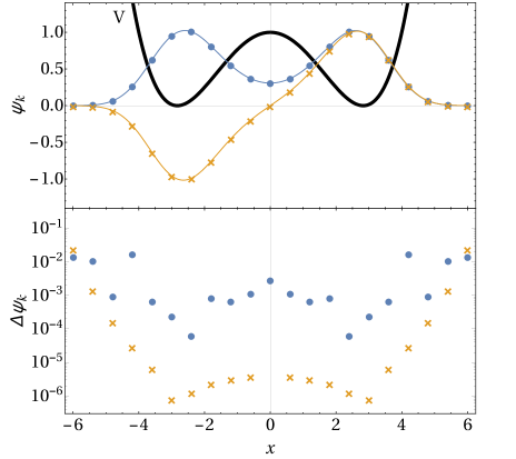
Figure 6: Comparison of the wavefunctions (normalized as in eq. (4.1) at $x_{0}=2\sqrt{2}$) for the first two levels of the symmetric double-well potential with $\lambda=1/32$ . Those computed in EPT with $N=200$ are indicated by blue bullets (ground state) and orange crosses (first state) while the ones computed using the RR method are indicated by solid curves.

As far as we know, the convergence of series related to observables other than energy eigenvalues have been poorly studied. This has motivated us to analyze the series associated to the wave functions $\phi_{k}(x;\lambda)$. We report in table 1 the values of $\Delta\psi_{k}(x;\lambda)$ for the first three levels of the anharmonic oscillator, $\alpha=0$ in eq. (4.3), and the symmetric double well (4.10), for some values of $x$ at $\lambda=1$. Given the exponential decay of the wave function, larger values of $x$ are subject to an increasing numerical uncertainty and are not reported. The decrease in accuracy as the level number $k$ increases is also expected, since both the RR methods and SPT/EPT require more and more precision. In all the cases considered the Borel-Padé approximants are free of poles in the real positive $t$ axis. The results clearly indicate that EPT captures the full answer. For illustration in fig. 6 we plot $\psi_{0,1}$ and $\Delta\psi_{0,1}$ at $\lambda=1/32$.

4.3 Supersymmetric Double Well

We now turn to the notable tilted double-well potential

$$V(x;\lambda)=\frac{\lambda}{2}\Big{(}x^{2}-\frac{1}{4\lambda}\Big{)}^{2}+\sqrt{\lambda}x\,.$$ (4.15)

This is the exact quantum potential that one obtains from the supersymmetric version of the double well when the fermionic variables are integrated out. As it is well known, the ground state energy $E_{0}=0$ to all orders in SPT due to supersymmetry. At the non-perturbative level, however, $E_{0}\neq 0$ because supersymmetry is dynamically broken [37]. Due to the absence of perturbative contributions in SPT, the supersymmetric double-well is the ideal system where to test EPT. It is also one of the simplest system where a perturbative expansion is Borel resummable (being identically zero), but the sum does not converge to the exact value.

Different authors have invoked complex instantons to reproduce $E_{0}$ [38, 39]. Their argument is essentially based on the observation that the entire quantum tilted potential (4.15) does not admit other real saddles that can contribute to the ground state energy. Note however that the perturbation theory in $\lambda$ corresponds to the expansion around the saddle points of the classical action. Since the tilt in eq. (4.15) is quantum in nature, the saddle-points of this system are the same as the ones of the symmetric double-well. In particular, real instantons occur, meaning that the path integral is on a Stokes line. The instanton contributions to $E_{0}$ have been extensively studied in ref.[40], where the first nine terms of the perturbative series around the 1-instanton saddle have been computed using a generalized Bohr-Sommerfeld quantization formula [41]. As expected, this expansion agrees very well with the numerical calculation at small coupling, while it breaks down when $\lambda$ approaches one since the perturbative expansion of more and more instantons need to be properly included.

Note that the expansion around the saddle-points of the full action corresponds to treat the whole potential (4.15) as classical. This means that the coefficient of the linear tilt is rescaled by a factor $\lambda_{0}/\lambda$ to satisfy eq. (3.15). The resulting potential, which leads to an alternative perturbative expansion in $\lambda$ (APT), reads

$$V_{\rm APT}=\frac{\lambda}{2}\Big{(}x^{2}-\frac{1}{4\lambda}\Big{)}^{2}+\frac{\lambda_{0}}{\sqrt{\lambda}}x\,.$$ (4.16)

The original result is recovered by setting $\lambda=\lambda_{0}$. This expansion for the ground state energy is no longer supersymmetric, but according to the discussion in subsec. 3.2 is Borel resummable to the exact result.

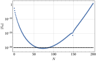
Figure 7: The partial sum (4.17) of APT for the potential (4.16) as a function of $N$ for $\lambda=1/200$. The black dashed line corresponds to the exact ground state energy as computed using RR methods.

We show in fig. 7 the partial sums

$$S_{N}=\sum_{k=1}^{N}c_{k}\lambda^{k}$$ (4.17)

of the coefficients of APT as a function of $N$ for $\lambda=1/200$. The dashed line represents the exact ground state energy. While each term in perturbation theory is non-vanishing, cancellations make the size of the truncated sum to decrease until $N\approx N_{\rm Best}=74$, where it approaches the expected non-perturbative answer. For larger values of $N$ the series starts diverging, though Borel resummation reconstructs the right value with a precision of ${\cal O}(10^{-3})$ using $N=200$ terms. The feature appearing around $N=150$ is due to the change of sign of the truncated sum. Indeed the sign of the coefficients $c_{k}$ oscillates with a long period ${\cal O}(150)$ since at weak coupling the tilt of the double-well potential is small and complex singularities of the Borel plane are close to the real axis (see fig. 4).

Analogously to the previous cases we can also introduce an EPT for which all the observable are Borel resummable. For this purpose we consider the auxiliary potential

$$V_{0}=\frac{1}{32\lambda}+\frac{\lambda_{0}}{2}x^{2}+\frac{\lambda}{2}x^{4}\,,\quad\quad V_{1}=\frac{x}{\sqrt{\lambda}}-\left(1+\frac{1}{2\lambda_{0}}\right)\frac{x^{2}}{2}\,,$$ (4.18)

where $V_{1}$ includes the quantum tilt $x$ and the quadratic $x^{2}$ term necessary to recover the original potential. The specific decomposition (4.18) turns out to be numerically convenient for moderately small and large couplings.

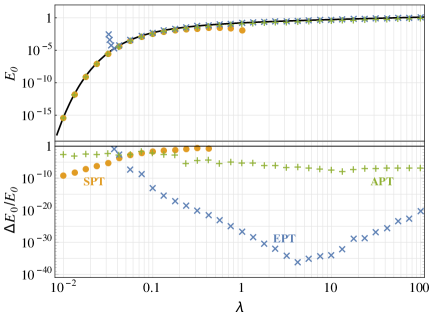
Figure 8: The ground state energy (top) and the relative error (bottom) as a function of the coupling $\lambda$ for the supersymmetric double well (4.15). The blue [green] crosses refer to EPT [APT] from the potential (4.18) [(4.16)] with $N=200$ series coefficients, the orange dots to SPT of ref.[40], with a truncated expansion up to the ninth order around the leading instanton. The black line corresponds to the exact result, computed by means of a Rayleigh-Ritz method.

In fig. 8 we show a comparison between the various perturbative estimates of $E_{0}$ and the numerical RR one as a function of the coupling constant. As expected, at small coupling SPT provides the best estimate. In fact it encodes analytically the leading instanton effect providing the asymptotic value of $E_{0}$ at $\lambda\to 0$. However, already at moderately small couplings both APT and EPT are able to resolve the leading instanton effects with a good accuracy. At moderate and strong coupling the instanton computation quickly breaks down, while both APT and EPT work extremely well. In particular the accuracy of EPT strongly increases with $\lambda$ up to $\lambda\sim 4$. For larger values of the coupling the accuracy drops, but it remains remarkable. For $\lambda\sim 10^{2}$ we have an accuracy $\sim 10^{-20}$ with 200 orders of perturbation theory. It is amazing how a perturbative computation can work so efficiently at strong coupling!

4.4 False Vacuum

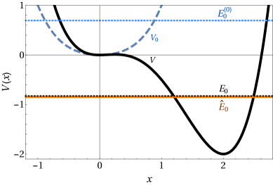
Figure 9: Plots of the potential (4.19) (solid black curve) and the associated potential $V_{0}$ in eq. (4.20) (dashed curve) with $\lambda=1$. The dashed blue line corresponds to the ground state energy associated to $V_{0}$, the solid red and the dashed black ones are the ground state energy of the potential (4.19) obtained from EPT and RR methods, respectively.

We now consider the potential (4.3) with $|\alpha|>1$. In this case $x=0$ is no longer the absolute minimum, and we are effectively expanding around a false vacuum. Clearly SPT is non-Borel resummable in this case, given the presence of other real instantons. The perturbative expansion around the false vacuum does not contribute at all to $E_{0}$, which, as we saw, is entirely reconstructed by the expansion around the true vacuum. Still the EPT around the false vacuum defined by the potential (4.5) is able to recover the (true) ground state energy.

In fig. 9 we show the shape of the original potential $V$ for $\alpha=-3/2$

$$V(x;\lambda)=\frac{1}{2}x^{2}-\frac{3}{2}\sqrt{\lambda}x^{3}+\frac{\lambda}{2}x^{4}\,,$$ (4.19)

and the corresponding exact ground state energy $E_{0}\approx-0.828$ at $\lambda=1$. We also show the potential $V_{0}$ used in EPT

$$V_{0}=\frac{1}{2}x^{2}+\frac{\lambda}{2}x^{4}\,,$$ (4.20)

with the would-be ground state energy $E_{0}^{(0)}\approx 0.696$. Using EPT with $N=280$ orders such value moves to $\hat{E}_{0}\approx-0.847$. Although the accuracy is not comparable to that obtained in the previous cases, it is remarkable that one is able to compute the energy of the true vacuum starting from a perturbative expansion around a false vacuum.

4.5 Degenerate Saddle Points: Pure Anharmonic Oscillators

In this subsection we discuss how to use EPT to address the infinitely coupled systems described by potentials with degenerate saddle points. Consider for example the pure anharmonic oscillators with potentials of the form

$$V(x)=2^{\ell}x^{2\ell}\,,\qquad\ell\in\mathbb{N}^{+}\,.$$ (4.21)

The factor $2^{\ell}$ is such that, modulo a trivial rescaling, the Hamiltonian is of the form $p^{2}+x^{2\ell}$ which is the conventional normalizaton used in the literature for this class of models. Pure anharmonic oscillators are intrinsically strongly coupled and can be obtained as the $\lambda\rightarrow\infty$ limit of their corresponding ordinary massive anharmonic oscillators after the rescaling $x\rightarrow\lambda^{-1/2(1+\ell)}x$. The potentials (4.21) are convex with a degenerate minimum at $x=0$. In the absence of a quadratic mass term, perturbation theory cannot be used. The energy eigenvalues $E_{k}^{(2\ell)}$ of these systems have instead been studied using Rayleigh-Ritz methods (see e.g. ref.[42]), Thermodynamic Bethe Ansatz (TBA) [43] or a Wentzel Kramers Brillouin (WKB) approximation [44] (see also ref.[45] for a more modern perspective). In the WKB approximation one considers a series expansion in $1/k$, $k$ being the quantum number level. It was found in refs.[44, 45] that the asymptotic series of the WKB expansion, where classical real trajectories in phase space are considered, does not reproduce the correct result. A better accuracy is achieved by adding in the WKB quantization formula the contribution of complex trajectories in phase space. However, there are an infinite number of them and a parametrically high accuracy could be obtained only by resumming all the infinite complex trajectories.

In terms of Lefschetz thimbles, the potentials (4.21) have a degenerate saddle for which our considerations do not apply. A possibility is to add a mass term $\epsilon x^{2}$ to eq. (4.21), compute the energy levels $E_{k}^{(2\ell)}(\epsilon)$ and extrapolate the result for $\epsilon\rightarrow 0$. By choosing $\epsilon>0$ we are guaranteed that $E_{k}^{(2\ell)}(\epsilon)$ are Borel resummable for any $\epsilon$ and no (real or complex) non-perturbative contributions are expected. We have verified this expectation by computing the ground state energy $E_{0}^{(4)}(\epsilon)$ for the pure quartic oscillator for smaller and smaller values of $\epsilon$ (using the Padé-Borel method) and have found that the extrapolated value $E_{0}^{(4)}$ converges to the exact value.

The same result can be found with much greater accuracy and efficiency using EPT without taking any extrapolation. Consider the auxiliary family of potentials defined as

$$V_{0}=\lambda^{\ell-1}2^{\ell}x^{2\ell}+\sum_{j=1}^{\ell-1}c_{j}\lambda^{j-1}x^{2j}\,,\qquad V_{1}=-\frac{1}{\lambda_{0}}\sum_{j=1}^{\ell-1}c_{j}\lambda^{j-1}x^{2j}\,,$$ (4.22)

such that at $\lambda=\lambda_{0}=1$ the potential in eq. (4.21) is recovered. By a proper choice of the $\ell-1$ coefficients $c_{j}$, $V_{0}$ has a unique non-degenerate minimum at $x=0$ and perturbation theory is well-defined.

For the pure quartic case $\ell=2$, by choosing $c_{1}=2$ in eq. (4.22) and by using only the first ten orders of EPT we get $E_{0}^{(4)}\simeq 1.060362$, which is more accurate than the value in tab. 2 of ref.[45], obtained using 320 orders in the WKB expansion with the inclusion of the leading complex saddles. The accuracy is easily improved using more coefficients of the perturbative expansion.

$k$	$E_{k}^{(4)}$	$\Delta E_{k}^{(4)}/E_{k}^{(4)}$	$E_{k}^{(6)}$	$\Delta E_{k}^{(6)}/E_{k}^{(6)}$
0	1.0603620904	$3\cdot 10^{-45}$	0.5724012268	$2\cdot 10^{-19}$
1	3.7996730298	$2\cdot 10^{-44}$	2.1692993557	$3\cdot 10^{-19}$
2	7.4556979379	$9\cdot 10^{-37}$	4.5365422804	$9\cdot 10^{-17}$
3	11.6447455113	$4\cdot 10^{-36}$	7.4675848174	$7\cdot 10^{-16}$
4	16.2618260188	$4\cdot 10^{-36}$	10.8570827110	$2\cdot 10^{-16}$

Table 2: Energy eigenvalues $E_{k}^{(2\ell)}$ and the corresponding accuracies $\Delta E_{k}^{(2\ell)}/E_{k}^{(2\ell)}$ of the first five levels of the pure anharmonic $x^{4}$ and $x^{6}$ potentials, computed using EPT with $N=200$. Only the first ten digits after the comma are shown (no rounding on the last digit).

We have computed in this way the $E_{k}^{(2\ell)}$ for different values of $\ell$ and $k$, as well as the associated wave-functions $\psi_{k}^{(2\ell)}(x)$ for some values of $x$. In all cases we found excellent agreement between our results and those obtained with RR methods.

For illustration we report in tab. 2 the accuracies for the energy levels of the first five states of the pure $x^{4}$ and $x^{6}$ oscillators computed comparing EPT to the results from RR methods. We used $N=200$ orders of perturbation theory and in eq. (4.22) we chose $c_{1}=2$ for $\ell=2$ and $c_{1}=4$, $c_{2}=2$ for $\ell=3$. Notice the accuracy of $E_{0}^{(4)}$ up to 45 digits! At fixed $N$, similarly to the RR method, the accuracy decreases as the energy level and the power $\ell$ in eq. (4.21) increase (in contrast to the WKB method where the opposite occurs) All the energy eigenvalues reported in tab. 2 are in agreement with those reported in tab. 1 of ref.[42], tab. I and II of ref.[43] and tab. 2 of ref.[45], in all cases computed with less precision digits than our results. The accuracy of our results sensibly depend on the choice of the coefficients $c_{j}$ in eq. (4.22). We have not performed a systematic search of the optimal choice that minimizes the errors, so it is well possible that at a fixed order $N$ a higher accuracy than that reported in tab. 2 can be achieved.

5 Conclusions and Future Perspectives in QFT

In this paper we have studied one-dimensional QM systems with bound-state potentials and discrete spectra. We characterized some of the conditions for the Borel summability of perturbation theory in QM. In particular when the potential admits only one critical point (minimum), we have shown that the loopwise expansion in the Euclidean path integral is Borel resummable and reproduces the full answer. Several known results in the literature about the Borel summability of certain QM systems, such as the quartic anharmonic oscillator [2, 3], are rederived and generalized in this new perspective.

We also explained why EPT—the modified perturbative expansion introduced in ref. [17]—is able to extend the above result to generic bound-state potentials. Remarkably, EPT encodes all the non-perturbative corrections of SPT, the standard semi-classical expansion including instantons, providing the full answer for any value of the coupling constant. In particular, EPT works at its best at strong coupling, where the high accuracy obtained confirms its validity. All complications occurring in SPT, related to the need of a resurgence analysis to make sense of otherwise ambiguous results, or of a highly non-trivial Lefschetz thimble decomposition of the path integral, are bypassed when using EPT. These points have been illustrated in details with several examples.

Our results can be extended in various directions. It would be interesting to understand if and how they can be obtained directly in Minkowski space where, contrary to the Euclidean case, one would always expect an infinite number of saddles to contribute. On the other hand the generalization to higher-dimensional QM systems with bound-state potentials should be straightforward.

The extension of our results to QFT is probably the most interesting. Possible complications arise both from UV and IR effects. As it is well-known, in contrast to QM, in QFT it is not enough to properly define the path integral measure to get a finite theory. The key point to address is understanding how the renormalization procedure needed to remove UV divergencies affects the Lefschetz thimble approach to the path integral.

The IR limit (i.e. infinite volume limit) is also more subtle than in QM because of possible phase transitions and spontaneous breaking of symmetries. Since in this case observables $O(\lambda)$ may no longer be analytic for any value of the coupling $\lambda$, it is not clear what will be the fate of the properties of perturbation theory and of the thimble decomposition.

Aside from the subtleties mentioned above, a naive extrapolation of our anharmonic potentials to scalar QFT would lead to the expectation that perturbation theory for superrenormalizable potentials with a single critical point are Borel resummable to the exact result. The proof of the Borel summability for the particular cases of the $\phi^{4}$ theories with a positive squared mass term in $d=2$ and $d=3$ [4, 5] seems to be compatible with this conjecture. The $\phi^{4}$ theory in $d=2$ seems the ideal laboratory to start exploring our ideas in the QFT framework. Indeed this is one of the simplest non-integrable QFT where UV divergencies can be removed by just normal ordering. In addition, in the infinite volume limit, it undergoes a second-order phase transition to a ${\bf Z}_{2}$-breaking phase in $d=2$ [46]. We hope to come back to the analysis of this model in the future.

On a more general perspective, by a proper analytic continuation in the space-time dimension, one might hope to put on firmer grounds the conjectured Borel summability of the $\epsilon$-expansion in the $\phi^{4}$ theory [11]. In QFT we will not have access to many terms in the perturbative expansion, and of course we cannot expect the degree of accuracy that is possible in QM. Nevertheless, computations of critical exponents in the three-dimensional Ising and vector $O(N)$ models have shown that an accuracy at the per mille level can be achieved at strong coupling $\epsilon=1$ by resumming (using Borel-Padé approximants, conformal mapping or other methods) the first few loops in perturbation theory [47]. More ambitious goals would be to extend our methods to QFT that are not Borel resummable, like gauge theories in $d=4$. Any progress in this direction would be of great interest.

We think that the results of this paper have opened a new perturbative window on strongly coupled physics.

Appendix A On the Finiteness of ${\cal B}_{-1/2}^{(\infty)}{\cal Z}$

In this appendix we report some checks we performed about the finiteness of the continuum limit of ${\cal B}_{-1/2}^{(N)}{\cal Z}(\lambda t)$. First of all, we consider the partition function of the harmonic oscillator. We discretize the path integral by cutting-off the real Fourier modes coefficients $c_{n}$ of $x(\tau)$:

$$x(\tau)=\sum_{k=0}^{N}c_{k}\eta_{k}\cos\frac{2\pi k\tau}{\beta}+\sum_{k=1}^{N}c_{-k}\eta_{k}\sin\frac{2\pi k\tau}{\beta}\,,\quad\eta_{k}=\frac{\sqrt{2-\delta_{k,0}}}{\sqrt{\beta}}\,.$$ (A.1)

The discretized action reads

$$S^{(N)}[x]=\int_{0}^{\beta}d\tau\,\left[\frac{1}{2}\dot{x}^{2}+\frac{1}{2}\omega^{2}x^{2}\right]=\frac{1}{2}\sum_{k=-N}^{N}\mu_{k}c_{k}^{2}\,,\qquad\mu_{k}\equiv\omega^{2}+\frac{(2\pi k)^{2}}{\beta^{2}}\,.$$ (A.2)

The path integral measure reads

$${\cal D}^{(N)}x(\tau)=\prod_{k=-N}^{N}N_{k}\,dc_{k}\,,\qquad N_{k}\equiv\left\{\begin{array}[]{c c c }\frac{|k|}{\beta}\sqrt{\frac{2\pi}{\lambda}}&&k\neq 0\\ \frac{1}{\beta\sqrt{2\pi\lambda}}&&k=0\end{array}\right.\,.$$ (A.3)

Introduce now a radial coordinate system defined as

$$c_{k}=\sqrt{\frac{2}{\mu_{k}}}\rho\,\hat{c}_{k}\,,\quad\sum_{k=-N}^{N}\hat{c}_{k}^{2}=1$$ (A.4)

where $\rho$ is the radius and the $\hat{c}_{k}$’s encode the standard parametrization of the unit $2N$-sphere in terms of its $2N$-angles, whose explicit form will not be needed. Using the expression (3.8) for the Borel-Le Roy function and the above results, we get

$${\cal B}_{-1/2}^{(N)}{\cal Z}_{0}(\lambda t) =\frac{\sqrt{\lambda t}}{\beta}\prod_{k=1}^{N}\left[\frac{2\pi k}{\beta}\right]^{2}\partial_{\lambda t}^{N}\int_{0}^{\infty}\frac{d\rho}{\rho}\,\Omega_{2N+1}\left[\prod_{k=-N}^{N}\frac{\rho}{\sqrt{\pi\mu_{k}}}\right]\delta(\rho^{2}-t\lambda)$$

$$=\frac{1}{\Gamma\left(N+\frac{1}{2}\right)}\sqrt{\lambda t}\,\partial_{\lambda t}^{N}(\lambda t)^{N-\frac{1}{2}}\frac{1}{\beta\omega}\prod_{k=1}^{N}\frac{1}{1+\left(\frac{\omega\beta}{2\pi k}\right)^{2}}$$

$$=\frac{1}{\Gamma\left(\frac{1}{2}\right)}\frac{1}{\beta\omega}\prod_{k=1}^{N}\frac{1}{1+\left(\frac{\omega\beta}{2\pi k}\right)^{2}}\,,$$ (A.5)

where $\Omega_{d}=2\pi^{d/2}/\Gamma(d/2)$ is the area of the unit $(d-1)$-dimensional sphere and we used the relation

$$\partial_{\lambda t}^{N}(\lambda t)^{N+p}=\frac{\Gamma(N+p+1)}{\Gamma(p+1)}(\lambda t)^{p}\,,$$ (A.6)

valid for any value of $p$. Notice how taking $N$ derivatives with respect to $\lambda t$ gives rise to an $N$-dependent Gamma function that compensates the one coming from the area of the unit-sphere. As expected, the dependence on $\lambda t$ disappears and the continuum limit gives the finite answer

$$\lim_{N\to\infty}{\cal B}_{-1/2}^{(N)}{\cal Z}_{0}(\lambda t)\equiv\lim_{N\to\infty}\frac{{\cal Z}_{0}^{(N)}}{\Gamma(1/2)}=\frac{{\cal Z}_{0}}{\Gamma\left(\frac{1}{2}\right)}\,,\quad\quad{\cal Z}_{0}=\frac{1}{2\sinh\left(\frac{\omega\beta}{2}\right)}\,,$$ (A.7)

which reproduces the known partition function ${\cal Z}_{0}$ of the harmonic oscillator after the integral over $t$ is performed.

An exact computation of ${\cal B}_{-1/2}^{(N)}{\cal Z}(\lambda t)$ is clearly out of reach in interacting QM systems. Yet, we can show that ${\cal B}_{-1/2}^{(\infty)}{\cal Z}(\lambda t)$ is finite to all orders in perturbation theory for polynomial potentials. It is useful to work out in detail the first order term of ${\cal B}_{-1/2}^{(N)}{\cal Z}(\lambda t)$ for the quartic anharmonic oscillator $V(x)=\omega^{2}x^{2}/2+x^{4}/4$. We have

$${\cal B}_{-1/2}^{(N)}{\cal Z}(\lambda t)={\cal Z}_{0}^{(N)}\frac{\sqrt{\lambda t}}{\pi^{N+\frac{1}{2}}}\partial_{\lambda t}^{N}\int_{0}^{\infty}d\rho\int d\Omega_{2N+1}\,\rho^{2N}\delta(\rho^{2}+\rho^{4}\xi-t\lambda)\,,$$ (A.8)

where ${\cal Z}_{0}^{(N)}$ is the discretized version of the harmonic oscillator partition function defined in eq.(A.7) and

$$\xi=\!\!\sum_{n,m,p,q=-N}^{N}\!\!\frac{\eta_{n}\eta_{m}\eta_{p}\eta_{q}}{\sqrt{\mu_{n}\mu_{m}\mu_{p}\mu_{q}}}\int_{0}^{\beta}\!\!d\tau(\hat{c}_{n}X_{n})(\hat{c}_{m}X_{m})(\hat{c}_{p}X_{p})(\hat{c}_{q}X_{q})\,,\quad X_{n}\equiv\left\{\begin{array}[]{c c }\cos\frac{2\pi n\tau}{\beta}\,,&n\geq 0\\ \sin\frac{2\pi n\tau}{\beta}\,,&n<0\end{array}\right.\,.$$ (A.9)

At linear order in $\lambda t$, once we expand the argument of the delta function, we get

$${\cal B}_{-1/2}^{(N)}{\cal Z}(\lambda t)={\cal Z}_{0}^{(N)}\frac{\sqrt{\lambda t}}{\pi^{N+\frac{1}{2}}}\partial_{\lambda t}^{N}\int_{0}^{\infty}\!\!d\rho\!\int d\Omega_{2N+1}\rho^{2N-1}(1-2\rho^{2}\xi)\delta[\rho-\sqrt{\lambda t}(1-\lambda t\xi/2)+\ldots]+{\cal O}(\lambda t)^{2}\,.$$ (A.10)

It is convenient to evaluate the integral over the angular variables $\hat{c}_{n}$ before the one in $d\tau$ appearing in eq. (A.9). This is easily obtained by using the following identity, valid in cartesian coordinates in any number of dimensions $d$:

$$\int\!d^{d}x\,x_{n}x_{m}x_{p}x_{q}f(x^{2})=\frac{(\delta_{nm}\delta_{pq}+\delta_{np}\delta_{mq}+\delta_{nq}\delta_{mp})}{d(d+2)}\int\!d^{d}x\,x^{4}f(x^{2})\,,\quad x^{2}=\sum_{k=1}^{d}x_{k}x_{k}\,,$$ (A.11)

from which it immediately follows, taking $d=2N+1$,

$$\int\!\!d\Omega_{2N+1}\hat{c}_{n}\hat{c}_{m}\hat{c}_{p}\hat{c}_{q}=\frac{(\delta_{nm}\delta_{pq}+\delta_{np}\delta_{mq}+\delta_{nq}\delta_{mp})}{(2N+1)(2N+3)}\Omega_{2N+1}=\frac{\pi^{N+\frac{1}{2}}}{2\Gamma(N+\frac{5}{2})}(\delta_{nm}\delta_{pq}+\delta_{np}\delta_{mq}+\delta_{nq}\delta_{mp}).$$ (A.12)

The integral over $d\tau$ is straightforward and after a bit of algebra we get

$$\int\!\!d\Omega_{2N+1}\xi=\frac{3\beta}{2}\frac{\pi^{N+\frac{1}{2}}}{\Gamma(N+\frac{5}{2})}({\cal G}^{(N)})^{2}\,,\quad{\cal G}^{(N)}\equiv\frac{1}{\beta}\sum_{k=-N}^{N}\frac{1}{\mu_{k}}\,.$$ (A.13)

Plugging eq. (A.13) in eq. (A.10) gives

$$\begin{split}{\cal B}_{-1/2}^{(N)}{\cal Z}(\lambda t)&={\cal Z}_{0}^{(N)}\Big{(}\frac{1}{\Gamma(1/2)}-\frac{3\beta}{4}\sqrt{\lambda t}\partial_{\lambda t}^{N}(\lambda t)^{N+1/2}\frac{N+3/2}{\Gamma(N+\frac{5}{2})}({\cal G}^{(N)})^{2}+{\cal O}(\lambda t)^{2}\Big{)}\\ &={\cal Z}_{0}^{(N)}\Big{(}\frac{1}{\Gamma(1/2)}-\frac{3\beta}{4}({\cal G}^{(N)})^{2}\frac{\lambda t}{\Gamma(3/2)}+{\cal O}(\lambda t)^{2}\Big{)}\,.\end{split}$$ (A.14)

In the continuum limit we have

$$\begin{split}\lim_{N\rightarrow\infty}{\cal B}_{-1/2}^{(N)}{\cal Z}(\lambda t)={\cal Z}_{0}\Big{(}\frac{1}{\Gamma(1/2)}-\frac{3}{4}\beta{\cal G}^{2}\frac{\lambda t}{\Gamma(3/2)}+{\cal O}(\lambda t)^{2}\Big{)}\,,\end{split}$$ (A.15)

where

$${\cal G}=\frac{1}{2\omega}\coth\frac{\beta\omega}{2}$$ (A.16)

is the particle propagator at $\tau=0$. After integrating over $t$, eq. (A.15) reproduces the first order perturbative correction to the partition function of the quartic anharmonic oscillator.

Finiteness of ${\cal B}_{-1/2}^{(N)}{\cal Z}$ as $N\rightarrow\infty$ to all orders is easily shown. For simplicity, we just keep track of the factors of $N$, neglecting all other parameters. At order $(\lambda t)^{k}$, after expanding the argument of the delta function, we get

$${\cal B}_{-1/2}^{(N)}{\cal Z}(\lambda t)|_{\lambda^{k}}\propto{\cal Z}_{0}^{(N)}\frac{\sqrt{\lambda t}}{\pi^{N+\frac{1}{2}}}\partial_{\lambda t}^{N}(\lambda t)^{N+k-1/2}N^{k}\!\int d\Omega_{2N+1}\xi^{k}\,.$$ (A.17)

The $4k$-generalization of eq. (A.11) gives

$$\int d\Omega_{2N+1}\xi^{k}\propto\frac{1}{N^{2k}}\Omega_{2N+1}\,.$$ (A.18)

Plugging eq. (A.18) in eq. (A.17) and using eq. (A.6) gives

$$\lim_{N\rightarrow\infty}{\cal B}_{-1/2}^{(N)}{\cal Z}(\lambda t)|_{\lambda^{k}}\propto\lim_{N\rightarrow\infty}{\cal Z}_{0}^{(N)}\frac{(\lambda t)^{k}}{\pi^{N+\frac{1}{2}}}\frac{\Gamma(N+k+1/2)}{\Gamma(k+1/2)}\frac{\Omega_{2N+1}}{N^{k}}\propto{\cal Z}_{0}\frac{(\lambda t)^{k}}{\Gamma(k+\frac{1}{2})}\,.$$ (A.19)

Similarly, we can prove the finiteness of the continuum limit to all orders in perturbation theory for any other interaction term of the form $g\,x^{2p}$. Recall that the loopwise parameter $\lambda$ corresponds to a coupling constant $g=\lambda^{p-1}$ and hence, for $p\neq 2$, the two are not identical. Taking that into account, the scaling in $N$ of ${\cal B}_{-1/2}^{(N)}{\cal Z}$ at order $g^{k}$ reads

$$\lim_{N\rightarrow\infty}{\cal B}_{-1/2}^{(N)}{\cal Z}(\lambda t)|_{g^{k}}\propto\lim_{N\rightarrow\infty}{\cal Z}_{0}^{(N)}\frac{\sqrt{\lambda t}}{\pi^{N+\frac{1}{2}}}\partial_{\lambda t}^{N}(\lambda t)^{N+(p-1)k-\frac{1}{2}}N^{k}\frac{\Omega_{2N+1}}{N^{pk}}\propto\frac{g^{k}t^{k(p-1)}}{\Gamma\left[(p-1)k+\frac{1}{2}\right]}\,,$$ (A.20)

and is finite. q.e.d.

Finiteness of ${\cal B}_{-1/2}^{(N)}{\cal Z}$ to all orders in perturbation theory for any polynomial potential term easily follows from the above results.

References

- [1] F. J. Dyson, “Divergence of perturbation theory in quantum electrodynamics,” Phys. Rev. 85 (1952) 631. doi:10.1103/PhysRev.85.631
- [2] J. J. Loeffel, A. Martin, B. Simon and A. S. Wightman, “Pade approximants and the anharmonic oscillator,” Phys. Lett. B 30 (1969) 656. doi:10.1016/0370-2693(69)90087-2
- [3] B. Simon and A. Dicke, “Coupling constant analyticity for the anharmonic oscillator,” Annals Phys. 58 (1970) 76. doi:10.1016/0003-4916(70)90240-X
- [4] J.P. Eckmann, J. Magnen and R. Sénéor, “Decay properties and borel summability for the Schwinger functions in theories”, Commun.Math. Phys. 39, 251 (1975). doi:10.1007/BF01705374
- [5] J. Magnen and R. Sénéor, “Phase Space Cell Expansion and Borel Summability for the Euclidean in Three-Dimensions Theory,” Commun. Math. Phys. 56 (1977) 237. doi:10.1007/BF01614211
- [6] J. Ecalle. 1981,“Les Fonctions Resurgentes”, vol. I - III Publ. Math. Orsay.
- [7] I. Aniceto, R. Schiappa and M. Vonk, “The Resurgence of Instantons in String Theory,” Commun. Num. Theor. Phys. 6 (2012) 339 doi:10.4310/CNTP.2012.v6.n2.a3 [arXiv:1106.5922 [hep-th]].
- [8] M. Mariño, “Lectures on non-perturbative effects in large gauge theories, matrix models and strings,” Fortsch. Phys. 62 (2014) 455 doi:10.1002/prop.201400005 [arXiv:1206.6272 [hep-th]].
- [9] D. Dorigoni, “An Introduction to Resurgence, Trans-Series and Alien Calculus,” arXiv:1411.3585 [hep-th].
- [10] L. N. Lipatov, “Divergence of the Perturbation Theory Series and the Quasiclassical Theory,” Sov. Phys. JETP 45 (1977) 216 [Zh. Eksp. Teor. Fiz. 72 (1977) 411].
- [11] E. Brezin, J. C. Le Guillou and J. Zinn-Justin, “Perturbation Theory at Large Order. 1. The phi**2N Interaction,” Phys. Rev. D 15 (1977) 1544. doi:10.1103/PhysRevD.15.1544
- [12] E. Brezin, J.-C. Le Guillou and J. Zinn-Justin, “Perturbation Theory at Large Order. 2. Role of the Vacuum Instability,” Phys. Rev. D 15 (1977) 1558. doi:10.1103/PhysRevD.15.1558
- [13] E. Brezin, G. Parisi and J. Zinn-Justin, “Perturbation Theory at Large Orders for Potential with Degenerate Minima,” Phys. Rev. D 16 (1977) 408. doi:10.1103/PhysRevD.16.408
- [14] E. Witten, “Analytic Continuation Of Chern-Simons Theory,” AMS/IP Stud. Adv. Math. 50 (2011) 347 [arXiv:1001.2933 [hep-th]].
- [15] E. Witten, “A New Look At The Path Integral Of Quantum Mechanics,” arXiv:1009.6032 [hep-th].
- [16] D. Harlow, J. Maltz and E. Witten, “Analytic Continuation of Liouville Theory,” JHEP 1112 (2011) 071 doi:10.1007/JHEP12(2011)071 [arXiv:1108.4417 [hep-th]].
- [17] M. Serone, G. Spada and G. Villadoro, “Instantons from Perturbation Theory,” Phys. Rev. D 96 (2017) no.2, 021701 doi:10.1103/PhysRevD.96.021701 [arXiv:1612.04376 [hep-th]].
- [18] Y. Tanizaki and T. Koike, “Real-time Feynman path integral with Picard–Lefschetz theory and its applications to quantum tunneling,” Annals Phys. 351 (2014) 250 doi:10.1016/j.aop.2014.09.003 [arXiv:1406.2386 [math-ph]].
- [19] W. E. Caswell, “Accurate Energy Levels for the Anharmonic Oscillator and a Summable Series for the Double Well Potential in Perturbation Theory,” Annals Phys. 123 (1979) 153, doi:10.1016/0003-4916(79)90269-0.
- [20] G.H. Hardy, “Divergent Series ”, Oxford University Press, 1973.
- [21] A. D. Sokal, “An Improvement Of Watson’s Theorem On Borel Summability,” J. Math. Phys. 21 (1980) 261. doi:10.1063/1.524408
- [22] A. Vainshtein, “Decaying Systems and Divergence of the Series of Perturbation Theory”, Novosibirsk Institute of Nuclear Physics Report, December 1964, published in “Continuous advances in QCD. Proceedings, Conference, Minneapolis, USA, May 17-23, 2002,” K.A. Olive, M.A. Shifman and M.B. Voloshin, editors.
- [23] C. M. Bender and T. T. Wu, “Anharmonic oscillator. 2: A Study of perturbation theory in large order,” Phys. Rev. D 7 (1973) 1620. doi:10.1103/PhysRevD.7.1620
- [24] M. V. Berry and C.J. Howls, “Hyperasymptotics for Integrals with Saddles”, Proceedings: Mathematical and Physical Sciences Vol. 434, No. 1892 (Sep. 9, 1991), pp. 657-675.
- [25] C. J. Howls, “Hyperasymptotics for Multidimensional Integrals, Exact Remainder Terms and the Global Connection Problem.” Proceedings: Mathematical, Physical and Engineering Sciences, vol. 453, no. 1966, 1997, pp. 2271-2294. www.jstor.org/stable/53139.
- [26] S. Gukov, M. Mariño and P. Putrov, “Resurgence in complex Chern-Simons theory,” arXiv:1605.07615 [hep-th].
- [27] Interestingly enough, a precursor of eq.(3.3) already appears in section 5 of G. ’t Hooft, “Can we make sense out of Quantum Chromodynamics?”, lectures given at the Ettore Majorana Int. School of Subnuclear Physics, Erice, July 1977. Publ. in “The Why’s on Subnuclear Physics”. Ed. by A. Zichichi, Plenum, New York/London, 943.
- [28] J. Milnor, “Morse Theory” (1963), Princeton University Press - ISBN 0-691-08008-9.
- [29] S. Graffi, V. Grecchi and B. Simon, “Borel summability: Application to the anharmonic oscillator,” Phys. Lett. B 32 (1970) 631. doi:10.1016/0370-2693(70)90564-2
- [30] Wolfram Research, Inc., Mathematica, Champaign, IL (2016).
- [31] T. Sulejmanpasic and M. Ünsal, “Aspects of Perturbation theory in Quantum Mechanics: The BenderWu Mathematica package,” arXiv:1608.08256 [hep-th].
- [32] C. M. Bender and T. T. Wu, “Large order behavior of Perturbation theory,” Phys. Rev. Lett. 27 (1971) 461. doi:10.1103/PhysRevLett.27.461
- [33] P. Vieira, Mathematica Summer School on Theoretical Physics - http://msstp.org
- [34] J. J. Loeffel, Saclay Report DPh-.T/76-20, unpublished.
- [35] J. C. Le Guillou and J. Zinn-Justin, “Critical Exponents from Field Theory,” Phys. Rev. B 21 (1980) 3976. doi:10.1103/PhysRevB.21.3976
- [36] U. D. Jentschura and J. Zinn-Justin, “Higher order corrections to instantons,” J. Phys. A 34 (2001) L253 doi:10.1088/0305-4470/34/18/101 [math-ph/0103010].
- [37] E. Witten, “Dynamical Breaking of Supersymmetry,” Nucl. Phys. B 188 (1981) 513. doi:10.1016/0550-3213(81)90006-7
- [38] I. I. Balitsky and A. V. Yung, “Instanton Molecular Vacuum in Supersymmetric Quantum Mechanics,” Nucl. Phys. B 274, 475 (1986).
- [39] A. Behtash, G. V. Dunne, T. Schäfer, T. Sulejmanpasic and M. Ünsal, “Complexified path integrals, exact saddles and supersymmetry,” Phys. Rev. Lett. 116 (2016) no.1, 011601 doi:10.1103/PhysRevLett.116.011601 [arXiv:1510.00978 [hep-th]].
- [40] U. D. Jentschura and J. Zinn-Justin, “Instantons in quantum mechanics and resurgent expansions,” Phys. Lett. B 596 (2004) 138 doi:10.1016/j.physletb.2004.06.077 [hep-ph/0405279].
- [41] J. Zinn-Justin, “Instantons in Quantum Mechanics: Numerical Evidence for a Conjecture,” J. Math. Phys. 25, 549 (1984); see also J. Zinn-Justin, “Quantum Field Theory and Critical Phenomena”, chapter 43, Oxford Science Publications, fourth edition (2002).
- [42] H. Taseli, “Accurate computation of the energy spectrum for potentials with multiminima”, Int. J. Quant.Chem. 46 (1993) 319.
- [43] P. Dorey and R. Tateo, “Anharmonic oscillators, the thermodynamic Bethe ansatz, and nonlinear integral equations,” J. Phys. A 32 (1999) L419 doi:10.1088/0305-4470/32/38/102 [hep-th/9812211].
- [44] R. Balian, G. Parisi and A. Voros, “Discrepancies from asymptotic series and their relation to complex classical trajectories,” Phys. Rev. Lett. 41, 1141 (1978), Erratum Phys. Rev. Lett. 41, 1627 (1978). For a more extensive analysis, see also A. Voros, “The return of the quartic oscillator. The complex WKB method”, Ann. Inst. H. Poincaré A 39 (1983) 211.
- [45] A. Grassi, M. Mariño and S. Zakany, “Resumming the string perturbation series,” JHEP 1505 (2015) 038 doi:10.1007/JHEP05(2015)038 [arXiv:1405.4214 [hep-th]].
- [46] S. J. Chang, “The Existence of a Second Order Phase Transition in the Two-Dimensional phi**4 Field Theory,” Phys. Rev. D 13 (1976) 2778 Erratum: [Phys. Rev. D 16 (1977) 1979]. doi:10.1103/PhysRevD.13.2778, 10.1103/PhysRevD.16.1979
- [47] For a review see e.g. A. Pelissetto and E. Vicari, “Critical phenomena and renormalization group theory,” Phys. Rept. 368 (2002) 549 doi:10.1016/S0370-1573(02)00219-3 [cond-mat/0012164].