Agent Failures in All-Pay Auctions

Abstract

All-pay auctions, a common mechanism for various human and agent interactions, suffers, like many other mechanisms, from the possibility of players’ failure to participate in the auction. We model such failures, and fully characterize equilibrium for this class of games, we present a symmetric equilibrium and show that under some conditions the equilibrium is unique. We reveal various properties of the equilibrium, such as the lack of influence of the most-likely-to-participate player on the behavior of the other players. We perform this analysis with two scenarios: the sum-profit model, where the auctioneer obtains the sum of all submitted bids, and the max-profit model of crowdsourcing contests, where the auctioneer can only use the best submissions and thus obtains only the winning bid.

Furthermore, we examine various methods of influencing the probability of participation such as the effects of misreporting one’s own probability of participating, and how influencing another player’s participation chances changes the player’s strategy.

1 Introduction

Auctions have been the focus of much research in economics, mathematics and computer science, and have received attention in the AI and multi-agent communities as a significant tool for resource and task allocation. Beyond explicit auctions, as performed on the web (e.g., eBay) and in auction houses, auctions also model various real-life situations in which people (and machines) interact and compete for some valuable item. For example, companies advertising during the U.S. Superbowl are, in effect, bidding to be one of the few remembered by the viewer, and are thus putting in tremendous amounts of money in order to create a memorable and unique event for the viewer, overshadowing the other advertisers.

A particularly suitable auction for modeling various scenarios in the real world is the all-pay auction. In this type of auction, all participants announce bids, and all of them pay those bids, while only the highest bid wins the product. Candidates applying for a job are, in a sense, participating in such a bidding process, as they put in time and effort preparing for the job interview, while only one of them is selected for the job. This is a max-profit auction, as the auctioneer (employer, in this case), receives only the top bid. In comparison, a workplace with an “employee of the month” competition is a sum-profit auctioneer, as it enjoys the fruits of all employees’ labour, regardless of who won the competition.

The explosion in mass usage of the web has enabled many more all-pay auction-like interactions, including some involving an extremely large number of participants. For example, various crowdsourcing contests, such as the Netflix challenge, involve many participants putting in effort, with only the best performing one winning a prize. Similar efforts can be seen throughout the web, in TopCoder.com, Amazon Mechanical Turk, Bitcoin mining and other frameworks.

However, despite the research done on all-pay auctions in the past few years (DiPalantino and Vojnović, 2009; Chawla et al., 2012; Lev et al., 2013), some basic questions about all-pay auctions remain — in a full information setting, any equilibrium has bidders’ expected profit at $0$, raising, naturally, the question of why bidders would participate.

Several extensions to the all-pay auction model have been suggested in order to answer this question. For example, Lev et al. (2013) showed that allowing bidders to collude enables the cooperating bidders to have a positive expected profit, at the expense of others bidders or the auctioneer. This paper addresses this question by suggesting a model in which the bidders have a positive expected profit.

Furthermore, in all-pay auctions, the number of bidders is a crucial information in order to bid according to the equilibrium (Baye et al., 1996). Hence, the number of participants must be known to the bidder. We suggest a relaxation of this assumption by allowing the possibility of bidders’ failure, that is, there is a probability that a bidder will not be able to participate in the auction. Therefore, we assume that the number of potential bidders and the failure probability of every bidder are common knowledge, but not the exact number of participants.

As most large-scale all-pay auction mechanisms have variable participation, we believe this helps capture a large family of scenarios, particularly for online, web-based, situations and the uncertainty they contain. We propose a symmetric equilibrium for this situation, we show when it is unique and prove its various properties. Somewhat surprisingly, allowing failures makes the expected profit for bidders positive, justifying their participation.

We start by reviewing related work in Section 2. We then introduce the model with and without failures. In Section 4, we first examine the case where each bidder has a different failure probability. Next, in Section 5, we study the potential manipulations possible in this model, such as announcing a false probability (e.g., saying that you will put all your time into a TopCoder.com project) and changing the probability of others (e.g., sabotaging their car). Finally, in Section 6, as calculations in this general case are complex, we examine situations where bidders have the same failure probability (as is possible when weather or web server failure, for example, are the main determinant of participation), enabling us to detail more information about the equilibrium in this state. In those situations we examine the effectiveness of changing the participation probability for all the bidders (e.g., convincing a deity to make it snow or attacking the server).

2 Related Work

Initial research on all-pay auction was in the political sciences, modeling lobbying activities (Hillman and Riley, 1989), but since then, much analysis (especially that dealing with the Revenue Equivalence Theorem) has been done on game-theoretic auction theory. When bidders have the same value distribution for the item, Maskin and Riley (2003) showed that there is a symmetric equilibrium in auctions where the winner is the bidder with the highest bid. A significant analysis of all-pay auctions in full information settings was Baye et al. (1996), showing (aided by Hillman and Riley (1989)) the equilibrium states in various cases of all-pay auctions, and noting that most valuations (apart from the top two), are not relevant to the winner’s strategies.

More recent work has extended the basic model. Lev et al. (2013) addressed issues of mergers and collusions, while several others directly addressed crowdsourcing models. DiPalantino and Vojnović (2009) detailed the issues stemming from needing to choose one auction from several, and Chawla et al. (2012) dealt with optimal mechanisms for crowdsourcing.

The early major work on failures in auctions was McAfee and McMillan (1987), followed soon after by Matthews (1987), which introduced bidders who are not certain of how many bidders there will actually be at the auction. Their analysis showed that in first-price auctions (like our all-pay auction), risk averse bidders prefer to know the numbers, while it is the auctioneer’s interest to hide that number. In the case of neutral bidders (such as ours), their model claimed that bidders were unaffected by the numerical knowledge. Dyer et al. (1989) claimed that experiments that allowed “contingent” bids (i.e., one submits several bids, depending on the number of actual participants) supported these results. Menezes and Monteiro (2000) presented a model where auction participants know the maximal number of bidders, but not how many will ultimately participate. However, the decision in their case was endogenous to the bidder, and therefore a reserve price has a significant effect in their model (though ultimately without change in expected revenue, in comparison to full-knowledge models). In contrast to that, our model, which assumes a little more information is available to the bidders (they know the maximal number of bidders, and the probability of failure), finds that in such a scenario, bidders are better off not having everyone show up, rather than knowing the real number of contestants appearing. Empirical work done on actual auctions (Lu and Yang, 2003) seems to support some of our theoretical findings (though not specifically in all-pay auction settings).

In our settings, the failure probabilities are public information and the failures are independent. Such failures have also been studied in other game-theoretic fields. Meir et al. (2012) studied the effects of failures in congestion games, and showed that in some cases, the failures could be beneficial to the social welfare. Some earlier work focused on agent redundancy and agent failures in cooperative games, studying various solution concepts in such games (see, e.g.,  (Bachrach et al., 2011, 2014)).

3 Model

We consider an all-pay auction with a single auctioned item that is commonly valued by all the participants. This is a restricted case of the model in Baye et al. (1996), where players’ item valuation could be different.

Formally, we assume that each of the $n$ bidders issues a bid of $b_{i}$, $i=1,\ldots,n$, and all bidders value the item at $1$. The highest bidders win the item and divide it among themselves, while the rest lose their bid. Thus, bidder $i$’s utility from a combination of bids $(b_{1},\ldots,b_{n})$ is given by:

$$\pi_{i}(b_{1},\ldots,b_{n})=\begin{cases}\frac{1}{\left|\arg\max\limits_{j}b_{j}\right|}-b_{i}&i\in\arg\max\limits_{j}b_{j}\\ -b_{i}&i\notin\arg\max\limits_{j}b_{j}.\end{cases}$$ (1)

We are interested in a symmetric equilibrium, which in this case, without possibility of failure, is unique (Baye et al., 1996; Maskin and Riley, 2003). It is a mixed equilibrium with full support of $[0,1]$, so that each bidder’s bid is distributed in $[0,1]$ according to the same cumulative distribution function $F$, with the density function $f$ (since it is non-atomic, tie-breaking is not an issue). As we compare this case to that of no-failures, this is a case similar to that presented in Baye et al. (1996), where various results on the behavior of non-cooperative bidders have been provided. We briefly give an overview of the results without failures in Subsection 3.1.

When we allow bidders to fail, we assume that each of them has a probability of participating — $p_{i}\in[0,1]$. As a matter of convenience, we shall order the bidders according to their probabilities, so $0\leq p_{1}\leq p_{2}\leq\ldots\leq p_{n}\leq 1$. If a bidder fails to participate, its utility is $0$.

3.1 Auctions without Failures

The expected utility of any participant with a bid $b$ is:

$$\pi(b)=(1-b)\cdot Pr(winning\mid b)+(-b)\cdot Pr(losing\mid b)$$ (2)

where $Pr(winning\mid b)$ and $Pr(losing\mid b)$ are the probabilities of winning or losing the item when bidding $b$, respectively. In a symmetric equilibrium with $n$ players, each of the bidders chooses their bid from a single bid distribution with a probability density function $f_{n}(x)$ and a cumulative distribution function $F_{n}(x)$. A player who bids $b$ can only win if all the other $n-1$ players bid at most $b$, which occurs with probability $F_{n}^{n-1}(b)$. Thus, the expected utility of a player bidding $b$ is given by:

$$\pi\left(b\right)=\left(1-b\right)F_{n}^{n-1}\left(b\right)-b\left(1-F_{n}^{n-1}\left(b\right)\right)=F_{n}^{n-1}\left(b\right)-b.$$ (3)

The unique symmetric equilibrium is defined by the CDF $F_{n}(x)=x^{\frac{1}{n-1}}$ (Baye et al., 1996). This equilibrium has full support, and all points in the support yield the same expected utility to a player, $\pi(0)=\pi(x)$ for all $x\in[0,1]$. Since $\pi(0)=0$, this means that for all bids, $\pi\left(b\right)=0$. The various properties of an auction without failures can be found in Table 1 (Lev et al., 2013).

Variable	No Failures
Expected bid	$\frac{1}{n}$
$[$Variance$]$	$\left[\frac{1}{2n-1}-\frac{1}{n^{2}}\right]$
Bidder utility	$0$
$[$Variance$]$	$\left[\frac{n-1}{n(2n-1)}\right]$
Sum-profit principal utility	$1$
$[$Variance$]$	$\left[\frac{n}{2n-1}-\frac{1}{n}\right]$
Max-profit principal utility	$\frac{n}{2n-1}$
$[$Variance$]$	$\left[\frac{n(n-1)^{2}}{(3n-2)(2n-1)^{2}}\right]$

Table 1: The values, in expectation, of some of the variables when there is no possibility of failure

4 Every Bidder with Own Failure Probability

In this section, we assume that each bidder has its own probability for participating in the auction, with $0\leq p_{1}\leq\ldots\leq p_{n}\leq 1$. We can assume without loss of generality, that each bidder has a positive participating probability, that is, $p_{1}>0$. If this is not the case, we can remove from the auction the bidders with zero probability of participating.

4.1 Equilibrium Properties

Before we present a symmetric Nash equilibrium, we will characterize any Nash equilibrium.

Theorem 1.

In common values all-pay auction when the item value is $1$, if $p_{n-1}<1$ then there is a unique Nash equilibrium, in which the expected profit of every participating bidder is $\prod_{j=1}^{n-1}\left(1-p_{j}\right)$. Furthermore, there exists a continuous function $z:\left[0,1-\prod_{j=1}^{n-1}\left(1-p_{j}\right)\right]\rightarrow\left[0,1\right]$, such that when a bidder $i$, has a positive density over an interval, they bid according to $F_{i}\left(x\right)=\frac{z\left(x\right)+p_{i}-1}{p_{i}}$ over that interval, and if $p_{i}=p_{j}$ then $F_{i}=F_{j}$.

The proof of Theorem 1 can be found at the appendix. As Theorem 1 applies to the case where $p_{n-1}<1$, we now deal with the other case.

Theorem 2.

In common values all-pay auction when the item value is $1$, if $p_{n-1}=1$ then in every Nash equilibrium the expected profit of every participating bidder is $0$. At least two bidders with $p=1$ randomize over $\left[0,1\right]$ with each other player $i$ randomizing continuously over $\left(b_{i},1\right]$, $b_{i}>0$, and having an atomic point at $0$ of $\alpha_{i}\left(0\right)$. There exists a continuous function $z\left(x\right):\left[0,1\right]\rightarrow\left[0,1\right]$, such that when a bidder, $i$, has a positive density over an interval, they bid according to $F_{i}\left(x\right)=\frac{z\left(x\right)+p_{i}-1}{p_{i}}$ over that interval. For every $i$, the atomic point at $0$ is equals to $F_{i}\left(0\right)$.

When there are at least two bidders with $p=1$, the auction approaches the case without failures. The proof of Theorem 2 is a generalization of the case without agent failures (Baye et al., 1996), and can be found at the appendix.

4.2 Symmetric Equilibrium

We are now ready to present a symmetric Nash equilibrium, we assume that $0<p_{1}\leq\dots\leq p_{n}\leq 1$. If $p_{n-1}<1$, from Theorem 1 it follows that the equilibrium is unique. If $p_{n-1}=1$ the equilibrium is not unique, except for two bidders with $p=1$, every bidder can place an arbitrary atomic point at $0$. In the equilibrium that we present, every bidder has an atomic point at $0$ of $0$, and thus the equilibrium is symmetric.

In order to simplify the calculations, we add a “dummy” bidder, with index 0, and $p_{0}=0$, adding a bidder that surely will not participate in the auction, does not effect the other bidders and therefore does not influence the equilibrium.

We begin by defining a few helpful functions. First, we define $\lambda=\prod\limits_{j=1}^{n-1}\left(1-p_{j}\right)$, and we define the following expressions for all $1\leq k\leq n-1$:

$$H_{k}\left(x\right)=\left(\frac{\lambda+x}{\prod_{j=0}^{k-1}\left(1-p_{j}\right)}\right)^{\frac{1}{n-k}}$$ (4)

and

$$\underline{s}_{k}=\left(1-p_{k}\right)^{n-k}\prod_{j=0}^{k-1}\left(1-p_{j}\right)-\lambda.$$ (5)

For the virtual “0” index, we use $\underline{s}_{0}=1-\lambda$. Note that because the $p_{i}$’s are ordered, so are the $\underline{s}_{i}$’s: $1\geq\underline{s}_{0}\geq\underline{s}_{1}\geq\ldots\geq\underline{s}_{n-1}=0$.

We are now ready to define the CDFs for our equilibrium, for every bidder $1\leq i\leq n-1$:

$$F_{i}\left(x\right)=\begin{cases}1&\text{$x\geq\underline{s}_{0}$}\\ \frac{H_{1}\left(x\right)+p_{i}-1}{p_{i}}&x\in\left[\underline{s}_{1},\underline{s}_{0}\right)\\ \vdots&\vdots\\ \frac{H_{k}\left(x\right)+p_{i}-1}{p_{i}}&x\in\left[\underline{s}_{k},\underline{s}_{k-1}\right)\\ \vdots&\vdots\\ \frac{H_{i}\left(x\right)+p_{i}-1}{p_{i}}&x\in\left[\underline{s}_{i},\underline{s}_{i-1}\right)\\ 0&x<\underline{s}_{i}.\end{cases}$$ (6)

$F_{n}$, uniquely, while it is very similar to $F_{n-1}$ in its piecewise composition, has an atomic point at $0$ of $1-\frac{p_{n-1}}{p_{n}}$, so:

$$F_{n}\left(x\right)=\begin{cases}1&\text{$x\geq\underline{s}_{0}$}\\ \frac{H_{1}\left(x\right)+p_{n}-1}{p_{n}}&x\in\left[\underline{s}_{1},\underline{s}_{0}\right)\\ \vdots&\vdots\\ \frac{H_{k}\left(x\right)+p_{n}-1}{p_{n}}&x\in\left[\underline{s}_{k},\underline{s}_{k-1}\right)\\ \vdots&\vdots\\ \frac{H_{n-1}\left(x\right)+p_{n}-1}{p_{n}}&x\in\left(\underline{s}_{n-1},\underline{s}_{n-2}\right)\\ 1-\frac{p_{n-1}}{p_{n}}&x=0\\ 0&x<0.\end{cases}$$ (7)

Note that all CDFs are continuous and piecewise differentiable, and when $p_{i}=p_{j}$ it follows that $F_{i}=F_{j}$; therefore, this is a symmetric equilibrium. The intuition behind this equilibrium is that bidders that participate rarely will usually bid high, while those that frequently participate in auctions with less competition would more commonly bid low.

Theorem 3.

The strategy profile $F_{1},\dots,F_{n}$ defined in Equations (6) and (7) is an equilibrium, in which the expected profit of the bidders, if they haven’t failed is $\lambda$.

Proof.

In the course of proving this is indeed a equilibrium, we shall calculate the expected utility of the bidders when they participate.

When bidder $i$ bids according to this distribution, i.e., $x\in\left[\underline{s}_{k},\underline{s}_{k-1}\right)$ for $1\leq k\leq i$:

$$\begin{array}[]{rl}\pi_{i}\left(x\right)=&\left(1-x\right)\prod\limits_{j=1;j\neq i}^{n}\left(p_{j}F_{j}\left(x\right)+1-p_{j}\right)-x\left(1-\prod\limits_{j=1;j\neq i}^{n}\left(p_{j}F_{j}\left(x\right)+1-p_{j}\right)\right)\\ =&\prod\limits_{j=1;j\neq i}^{n}\left(p_{j}F_{j}\left(x\right)+1-p_{j}\right)-x\\ =&\prod\limits_{j=1}^{k-1}\left(p_{j}F_{j}\left(x\right)+1-p_{j}\right)\prod\limits_{j=k;j\neq i}^{n}\left(p_{j}F_{j}\left(x\right)+1-p_{j}\right)-x\\ =&\prod\limits_{j=1}^{k-1}\left(1-p_{j}\right)\prod\limits_{j=1;j\neq i}^{n}H_{k}\left(x\right)-x\\ =&\prod\limits_{j=1}^{k-1}\left(1-p_{j}\right)H_{k}\left(x\right)^{n-k}-x\\ =&\prod\limits_{j=1}^{k-1}\left(1-p_{j}\right)\left(\frac{\lambda+x}{\prod_{j=0}^{k-1}\left(1-p_{j}\right)}\right)-x\\ =&\lambda.\end{array}$$ (8)

If bidder $i$ bids outside their support, i.e., $x\in$ for $i+1\leq k\leq n-1$, the same equation becomes:

$$\begin{array}[]{rl}\pi_{i}(x)=&\prod\limits_{j=1;j\neq i}^{k-1}\left(1-p_{j}\right)\prod\limits_{j=k}^{n}H_{k}\left(x\right)-x\\ =&\prod\limits_{j=1;j\neq i}^{k-1}\left(1-p_{j}\right)\left(\frac{\lambda+x}{\prod_{j=1}^{k-1}(1-p_{j})}\right)^{\frac{n-k+1}{n-k}}-x\\ =&\frac{\lambda+x}{1-p_{i}}\left(\frac{\lambda+x}{\prod_{j=1}^{k-1}(1-p_{j})}\right)^{\frac{1}{n-k}}-x.\end{array}$$ (9)

Now,

$$\begin{array}[]{rl}x<&\underline{s}_{k-1}=\left(1-p_{k-1}\right)^{n-k+1}\prod_{j=1}^{k-2}\left(1-p_{j}\right)-\lambda\\ =&\left(1-p_{k-1}\right)^{n-k}\prod_{j=1}^{k-1}\left(1-p_{j}\right)-\lambda\end{array}$$ (10)

and hence $\lambda+x<(1-p_{k-1})^{n-k}\prod_{j=1}^{k-1}(1-p_{j})$. Plugging it all together,

$$\begin{array}[]{rl}\pi_{i}(x)<&\frac{\lambda+x}{1-p_{i}}\left(\frac{(1-p_{k-1})^{n-k}\prod_{j=1}^{k-1}(1-p_{j})}{\prod_{j=1}^{k-1}(1-p_{j})}\right)^{{}^{\frac{1}{n-k}}}-x\\ =&\frac{\lambda+x}{1-p_{i}}\left(1-p_{k-1}\right)-x\\ =&\left(\lambda+x\right)\frac{p_{i}-p_{k-1}}{1-p_{i}}+\lambda.\end{array}$$ (11)

Finally, as $i+1\leq k$, $p_{i}\leq p_{k-1}$, hence $p_{i}-p_{k-1}\leq 0$, and therefore $\pi_{i}(x)<\lambda$. ∎

4.3 Profits

When a bidder actually participates their expected utility, in the equilibrium, is $\lambda$, and therefore the overall expected utility for bidder $i$ is $p_{i}\lambda$ (which, naturally, decreases with $n$). Notice that, as is to be expected, a bidder’s profit rises the less reliable their fellow bidders are, or the fewer participants the auction has. However, the most reliable of the bidders does not affect the profits of the rest. If a bidder can set its own participation rate, if there is no bidder with $p_{j}=1$, that is the best strategy; otherwise, the optimal probability should be $\frac{1}{2}$, as that maximizes $p_{i}(1-p_{i})\prod_{j=1;j\neq i}^{n-1}(1-p_{j})$.

4.3.1 Expected Bid

In order to calculate the expected bid by each bidder, we need to calculate the bidders’ equilibrium PDF, for $1\leq i\leq n-1$:

$$f_{i}\left(x\right)=\begin{cases}0&\text{$x\geq\underline{s}_{0}$}\\ \frac{\left(\lambda+x\right)^{\frac{2-n}{n-1}}}{p_{i}\left(n-1\right)}&x\in\left[\underline{s}_{1},\underline{s}_{0}\right)\\ \vdots&\vdots\\ \frac{\left(\lambda+x\right)^{\frac{k+1-n}{n-k}}}{p_{i}\left(n-k\right)\prod_{j=0}^{k-1}\left(1-p_{j}\right)^{\frac{1}{n-k}}}&x\in\left[\underline{s}_{k},\underline{s}_{k-1}\right)\\ \vdots&\vdots\\ \frac{\left(\lambda+x\right)^{\frac{i+1-n}{n-i}}}{p_{i}\left(n-i\right)\prod_{j=0}^{i-1}\left(1-p_{j}\right)^{\frac{1}{n-i}}}\,\,\,\,&x\in\left[\underline{s}_{i},\underline{s}_{i-1}\right)\\ 0&x<\underline{s}_{i}\end{cases}$$ (12)

and $f_{n}\left(x\right)=\frac{p_{n-1}}{p_{n}}f_{n-1}\left(x\right)$. In the equilibrium, the expected bid of bidder $i$, for $1\leq i\leq n-1$ is:

$$\mathbb{E}\left[bid_{i}\right]=\sum_{k=1}^{i}\int\limits_{\underline{s}_{k}}^{\underline{s}_{k-1}}xf_{i}\left(x\right)\,\mathrm{d}x.$$ (13)

Theorem 4.

For every $1\leq i\leq n-1$:

$$\begin{split}\mathbb{E}\left[bid_{i}\right]=&\frac{1}{p_{i}}\left(\frac{1}{n}+\sum_{k=1}^{i}\frac{\left(1-p_{k}\right)^{n-k}\prod_{j=1}^{k}\left(1-p_{j}\right)}{\left(n-k\right)\left(n-k+1\right)}\right.\\ &\qquad\left.-\frac{\left(1-p_{i}\right)^{n-i}\prod_{j=1}^{i}\left(1-p_{j}\right)}{n-i}-p_{i}\lambda\right)\end{split}$$ (14)

and

$$\mathbb{E}\left[bid_{n}\right]=\frac{p_{n-1}}{p_{n}}\mathbb{E}\left[bid_{n-1}\right].$$ (15)

The expected bid decreases with $n$, indicating, as in the no-failure model, that as more bidders participate, the chance of losing increases, causing bidders to lower their exposure. The proof of Theorem 15 can be found at the appendix.

4.3.2 Auctioneer - Sum-Profit Model

In the equilibrium, the expected profit of the auctioneer in the sum-profit model is given by:

$$\mathbb{E}\left[AP\right]=\sum\limits_{i=1}^{n}p_{i}\mathbb{E}\left[bid_{i}\right].$$ (16)

When summing over all bidders, we receive a much simpler expression.

Theorem 5.

The sum-profit auctioneer’s equilibrium profits are:

$$\sum_{i=1}^{n}p_{i}\mathbb{E}\left[bid_{i}\right]=1-\lambda\left(1+\sum_{i=1}^{n-1}p_{i}\right).$$ (17)

In this case, growth with $n$ is monotonic increasing, and hence, any addition to $n$ is a net positive for the sum-profit auctioneer. The proof can be found at the appendix.

4.3.3 Auctioneer - Max-Profit Model

To calculate a max-profit auctioneer’s profits, we need to first define the max-profit auctioneer’s profits equilibrium CDF:

$$G\left(x\right)=\prod_{i=1}^{n}\left(p_{i}F_{i}\left(x\right)+1-p_{i}\right)$$ (18)

That is,

$$G\left(x\right)=\begin{cases}1&x\geq\underline{s}_{0}\\ \left(\lambda+x\right)^{\frac{n}{n-1}}&x\in\left[\underline{s}_{1},\underline{s}_{0}\right)\\ \vdots&\vdots\\ \frac{\left(\lambda+x\right)^{\frac{n-k+1}{n-k}}}{\prod_{j=0}^{k-1}\left(1-p_{j}\right)^{\frac{1}{n-k}}}\,\,\,&x\in\left[\underline{s}_{k},\underline{s}_{k-1}\right)\\ \vdots&\vdots\\ \frac{\left(\lambda+x\right)^{2}}{\prod_{j=0}^{n-2}\left(1-p_{j}\right)}&x\in\left[\underline{s}_{n-1},\underline{s}_{n-2}\right)\\ 0&x<0.\end{cases}$$ (19)

This is differentiable, and hence we can find $g\left(x\right)=\frac{\partial}{\partial x}G\left(x\right)$ and the max-profit auctioneer’s expected profit.

Theorem 6.

In the equilibrium, the max-profit auctioneer’s profits are:

$$\begin{split}\mathbb{E}\left[AP\right]=&\int\limits_{\underline{s}_{n-1}}^{\underline{s}_{0}}xg\left(x\right)\,\mathrm{d}x\\ =&\frac{n}{2n-1}-\lambda+\sum_{k=1}^{n-1}\left(\frac{(1-p_{k})^{2n-2k-1}\prod_{j=1}^{k}(1-p_{j})^{2}}{4(n-k)^{2}-1}\right).\end{split}$$ (20)

From Theorem 20 we can see that the max-profit auctioneer would prefer to minimize $\lambda$, have two reliable bidders ($p_{n}=p_{n-1}=1$), and the other $n-2$ bidders as unreliable as possible. The proof of Theorem 20 can be found at the appendix.

Example 1.

Consider how four bidders interact. Our bidders have participation probability of $p_{1}=\frac{1}{3}$, $p_{2}=\frac{1}{2}$, $p_{3}=\frac{3}{4}$ and $p_{4}=1$. Let us look at each bidder’s equilibrium CDFs:

$$\begin{array}[]{cl}F_{1}(x)=&\begin{cases}1&x\geq\frac{11}{12}\\ 3\left(\frac{1}{12}+x\right)^{\frac{1}{3}}-2\quad\enskip&x\in\left[\frac{23}{108},\frac{11}{12}\right)\\ 0&x<\frac{23}{108}\end{cases}\\ \\ F_{2}(x)=&\begin{cases}1&x\geq\frac{11}{12}\\ 2\left(\frac{1}{12}+x\right)^{\frac{1}{3}}-1&x\in\left[\frac{23}{108},\frac{11}{12}\right)\\ 2\left(\frac{3\left(\frac{1}{12}+x\right)}{2}\right)^{\frac{1}{2}}-1\;&x\in\left[\frac{1}{12},\frac{23}{108}\right)\\ 0&x<\frac{1}{12}\end{cases}\\ \\ F_{3}(x)=&\begin{cases}1&x\geq\frac{11}{12}\\ \frac{4}{3}\left(\frac{1}{12}+x\right)^{\frac{1}{3}}-\frac{1}{3}&x\in\left[\frac{23}{108},\frac{11}{12}\right)\\ \frac{4}{3}\left(\frac{3\left(\frac{1}{12}+x\right)}{2}\right)^{\frac{1}{2}}-\frac{1}{3}&x\in\left[\frac{1}{12},\frac{23}{108}\right)\\ 4\left(\frac{1}{12}+x\right)-\frac{1}{3}&x\in\left[0,\frac{1}{12}\right)\\ 0&x<0\end{cases}\\ \\ F_{4}(x)=&\begin{cases}1&x\geq\frac{11}{12}\\ \left(\frac{1}{12}+x\right)^{\frac{1}{3}}&x\in\left[\frac{23}{108},\frac{11}{12}\right)\\ \left(\frac{3\left(\frac{1}{12}+x\right)}{2}\right)^{\frac{1}{2}}\qquad\enskip&x\in\left[\frac{1}{12},\frac{23}{108}\right)\\ 3\left(\frac{1}{12}+x\right)&x\in\left(0,\frac{1}{12}\right)\\ \frac{1}{4}&x=0\\ 0&x<0\end{cases}\end{array}$$ (21)

A graphical illustration of the bidders’ CDFs and PDFs can be found in the appendix. The expected utility for bidder 1 is $0.027$, for expected bid of $0.518$; for bidder 2, $0.041$ for expected bid of $0.394$; for bidder 3, $0.0625$ for expected bid of $0.277$; and for the last bidder, $0.083$ for expected bid of $0.207$.

A sum-profit auctioneer will see an expected profit of $0.0784$, while a max-profit one will get, in expectation, $0.490$.

As a comparison, in the case where we do not allow failures, the CDF of the bidders is $x^{\frac{1}{3}}$ with expected bid of $\frac{1}{4}$ and expected utility of $0$. The expected profit of the sum-profit auctioneer is $1$, while the expected profit of the max-profit auctioneer is $\frac{4}{7}$.

5 False Identity and Sabotage

Algorithm 1 Optimal Bid

1:$i$, $r$, $p_{1},\dots,p_{n}$ and $p^{\prime}_{r}$

2:The optimal bid for bidder $i$

3:let $\lambda=\prod_{j=1}^{n-1}\left(1-p_{j}\right)$

4:for $k=1,\dots,\min\left\{i,r\right\}$ do

5:     if $\frac{1}{n-k}\in\left[p_{k-1},p_{k}\right]$ then

6:         let $x_{i,k}=\left(1-\frac{1}{n-k}\right)^{n-k}\prod_{j=1}^{k-1}\left(1-p_{j}\right)-\lambda$

7:         let $\pi_{i,k}=\frac{1}{n-k}\left(1-\frac{1}{n-k}\right)^{n-k-1}\prod_{j=1}^{k-1}\left(1-p_{j}\right)\frac{p_{r}-p^{\prime}_{r}}{p_{r}}+\lambda$

8:     else if $\frac{1}{n-k}<p_{k-1}$ then

9:         let $x_{i,k}=\underline{s}_{k-1}$

10:         let $\pi_{i,k}=p_{k-1}\left(1-p_{k-1}\right)^{n-k-1}\prod_{j=1}^{k-1}\left(1-p_{j}\right)\frac{p_{r}-p^{\prime}_{r}}{p_{r}}+\lambda$

11:     else if $\frac{1}{n-k}>p_{k}$ then

12:         let $x_{i,k}=\underline{s}_{k}$

13:         let $\pi_{i,k}=p_{k}\left(1-p_{k}\right)^{n-k-1}\prod_{j=1}^{k-1}\left(1-p_{j}\right)\frac{p_{r}-p^{\prime}_{r}}{p_{r}}+\lambda$

14:     end if

15:end for

16:let $j\in\arg\max_{k}\pi_{i,k}$

17:return $x_{i,k}$

Now, suppose our bidder can influence others’ perceptions, and create a false sense of its participation probability. What would its best strategy be, and how should the participation probability be altered? Any bid beyond $1-\lambda$ is sure to win, but as that would give profit of less than $\lambda$, which is less than the expected profit for non-manipulators, it is not worthwhile. Therefore, our bidder will bid in its support, with the expected profit being $\lambda$. However, our bidder may increase its expected profit by trying to portray its participation probability as being as low as possible, thus lulling the other bidders with a false sense of security. Of course, this reduces the payment to auctioneers of any type, and therefore, they would try to expose such manipulation.

More interesting is the possibility of a player’s changing another player’s participation probability by using sabotage; thus our bidder would be the only bidder knowing the real participation probability. Our bidder, $i$, sabotages bidder $r$, with a perceived participation probability of $p_{r}$, changing its real participation probability to $p^{\prime}_{r}$. Bidder $i$’s expected profit with bid $x$ is:

$$\pi_{i}(x)=\left(p^{\prime}_{r}F_{r}(x)+1-p^{\prime}_{r}\right)\prod_{j=1;j\neq i,r}^{n}\left(p_{j}F_{j}(x)+1-p_{j}\right).$$ (22)

The values of this function change according to the relation between $r$, $i$ and $x$. To find the optimal strategy for a bidder, we must examine all the options.

Theorem 7.

Let $p_{1},\dots,p_{n}$ be the announced participation probabilities, and let $p^{\prime}_{r}<p_{r}$ be bidder $r$ real participation probability. For every $i\neq r$, Algorithm 1 finds the optimal bid for bidder $i$.

To summarize, bidder $i$ best interest is to bid in the intersection of its support and bidder $r$’s support. Given the index of the saboteur bidder, the index of the sabotaged bidder, $p_{1},\dots,p_{n}$ and the participation probability after the sabotage, Algorithm 1 finds the optimal bid. The full proof can be found at the appendix.

6 Uniform Failure Probabilities

If we allow our bidders to have the same probability of failure (e.g., when failures stem from weather conditions), many of the calculations become more tractable, and we are able to further understand the scenario.

6.1 Bids

As this case is a particular instance of the general case presented above, we can calculate the expected equilibrium bid of every bidder and its variance.

Theorem 8.

The expected equilibrium bid of every bidder is:

$$\mathbb{E}\left[bid\right]=\frac{1}{np}\left(1-\lambda\left(1+p\left(n-1\right)\right)\right)$$ (23)

and the variance of the bid is:

$$\mathrm{Var}\left[bid\right]=\frac{1-(1-p)^{2n-1}}{(2n-1)p}-\frac{\left(1-(1-p)^{n}\right)^{2}}{n^{2}p^{2}}.$$ (24)

The expected bid and the variance are neither monotonic in $n$ nor in $p$.

6.2 Profits

We are now ready to examine the profits of all the parties, the bidder and the auctioneer, both in the sum-profit model and the max-profit model.

6.2.1 Bidder

From the general case we may deduce that expected equilibrium profit of every bidder is $p\left(1-p\right)^{n-1}$. Note the profit decreases as $n$ increases, and is maximized when $p=\frac{1}{n}$. We can now compute the variance of bidder profit.

Theorem 9.

The variance of the bidder equilibrium profit is:

$$\mathrm{Var}\left[BP\right]=\frac{n-1}{n\left(2n-1\right)}-\frac{\left(1-p\right)^{n}}{n}+\left(p+\frac{1}{2n-1}\right)\left(1-p\right)^{2n-1}.$$ (25)

And the variance is monotonic increasing in $p$.

6.2.2 Auctioneer - Sum-Profit Model

The expected bid of every bidder is $\frac{1}{pn}\left(1-\left(1-p\right)^{n-1}\left(1+p\left(n-1\right)\right)\right)$, therefore, the expected profit of the sum-profit auctioneer, in the equilibrium, is:

$$\begin{array}[]{rl}\mathbb{E}\left[AP\right]=&np\cdot\mathbb{E}\left[bid\right]\\ =&1-\left(1-p\right)^{n-1}\left(1+p\left(n-1\right)\right)\end{array}$$ (26)

which increases with $p$ and $n$. Therefore, the auctioneer best interest is to have as many bidders as possible. Note that as $n$ grows, the auctioneer’s expected revenue approaches that of the no-failure case. From Theorem 9 we get the variance of the auctioneer equilibrium profit in the sum profit model:

$$\begin{array}[]{rl}\mathrm{Var}\left[AP\right]=&np^{2}\mathrm{Var}\left[bid\right]\\ =&\frac{n\cdot p\left(1-(1-p)^{2n-1}\right)}{2n-1}-\frac{\left(1-(1-p)^{n}\right)^{2}}{n}.\end{array}$$ (27)

6.2.3 Auctioneer - Max-Profit Model

For the max-profit auctioneer, the expected profit in equilibrium is:

$$\frac{n}{2n-1}+\frac{n-1}{2n-1}\left(1-p\right)^{2n-1}-\left(1-p\right)^{n-1}$$ (28)

which is, monotonically increasing in $p$ and $n$ (for $n\geq 1$); for large enough $n$ it approaches the expected revenue in the no-failure case.

Theorem 10.

The variance of the auctioneer equilibrium profit in the max profit model is:

$$\begin{array}[]{rl}\mathrm{Var}\left[AP\right]=&\left(1-p\right)^{2n-2}-\frac{2n\left(1-p\right)^{n-1}}{2n-1}+\frac{n}{3n-2}-\frac{2\left(n-1\right)^{2}\left(1-p\right)^{3n-2}}{\left(3n-2\right)\left(2n-1\right)}\\ &-\left(\frac{n}{2n-1}+\frac{n-1}{2n-1}\left(1-p\right)^{2n-1}-\left(1-p\right)^{n-1}\right)^{2}.\end{array}$$ (29)

7 Conclusion and Discussion

Bidders failing to participate in auctions happen commonly, as people choose to apply to one job but not another, or to participate in the Netflix challenge but not a similar challenge offered by a competitor. Examining these scenarios enables us to understand certain fundamental issues in all-pay auctions. In the complete reliability, classic versions, each bidder has an expected revenue of $0$. In contrast, in a limited reliability scenario, such as the one we dealt with, bidders have positive expected revenue, and are incentivized to participate in the auction. Auctioneers, on the other hand, mostly lose their strong control of the auction, and no longer pocket almost all revenues involved in the auction. However, by influencing participation probabilities, max-profit auctioneers can effectively increase their revenue in comparison to the no-failure model.

The idea of the equilibrium we explored was that frequent participants could allow themselves to bid lower, as there would be plenty of contests where they would be one of the few participants, and hence win with smaller bids. Infrequent bidders, on the other hand, would wish to maximize the few times they participate, and therefore bid fairly high bids. As exists in the no-failure case as well, as more and more participants join, there is a concentration of bids at lower price points, as bidders are more afraid of the fierce competition. Hence, it is fairly easy to see in all of our results that as $n$ approached larger numbers, the various variables were closer and closer to their no-failure brethren.

There is still much left to explore in these models — not only more techniques of manipulation by bidders and potential incentives by auctioneers, but also further enrichment of the model. Currently, participation rates are not influenced by other bidders’ probability of participation, but, obviously, many scenarios in real-life have, effectively, a feedback loop in this regard. We assumed that the item is commonly valued by all the bidders and the cost of effort is common, which is not always the case. A future research could examine a more realistic model with heterogeneous costs or valuations. In our model the failure happened before the bidder placed their bid, but in other models the failure could happen after the bidders place their bid and before the auctioneer collected the bid. Finding a suitable model for such interactions, while an ambitious goal, might help us gain even further insight into these types of interactions.

Proof of Theorem 1

Before we prove Theorem 1, we begin with some notations; let $0<p_{1}\leq\dots\leq p_{n}\leq 1$ be the participation probability of the bidders. we assume that $p_{n-1}<1$, that is, at most one bidder surely participates in the auction. Let $F_{1},\dots F_{n}$, be a Nash equilibrium, such that $F_{i}$ denotes bidder $i$ bid distribution, where $F_{i}\left(x\right)=\Pr\left[bid_{i}\leq x\right]$, note that $F_{i}$ is a right-continuous function, and $F_{i}$ has a left-discontinuous point at $x$ if and only if the bidder has an atomic point at $x$.

First, we should note that there indeed exists an equilibrium, as the strategy profile $F_{1},\dots,F_{n}$ defined in Equations (6) and (7) is an equilibrium (see Theorem 3).

All the bidders value the item at $1$, hence every bidder has no incentive to bid more than $1$, bids less the $0$ are ruled out, that is, the bids are drawn from $\left[0,1\right].$

For every $i$ let

$$\alpha_{i}\left(x\right)=F_{i}\left(x\right)-\lim_{y\rightarrow x^{-}}F_{i}\left(y\right),$$ (30)

that is, $\alpha_{i}\left(x\right)>0$ if and only if bidder $i$ has an atomic point at $x$.

For every $i$ and $x$ denote by $\Pr\left(i\,\text{wins}\mid x\right)$ the probability that bidder $i$ wins the item, when they might share the item with other bidders, if all the other bidders are bidding according to $F_{-i}$; and denote by $\pi_{i}\left(x\right)$ the expected profit of bidder $i$ from bidding $x$. That is, $\Pr\left(i\,\text{wins}\mid x\right)=\pi_{i}\left(x\right)+x$.

Let $\underline{s}_{i}=\inf_{x}\left\{x\in\left[0,1\right]:F_{i}\left(x\right)>F_{i}\left(0\right)\right\}$ and $\overline{s}_{i}=\inf_{x}\left\{x\in\left[0,1\right]:F_{i}\left(x\right)=1\right\}$, the lower and upper bound of player $i$’s equilibrium bid distribution, excluding the atomic point at $0$ (if exists), respectively. Let $\pi_{i}^{*}$ be player $i$’s equilibrium profit, if they have not failed. We said that $F_{i}$ is strictly increasing at $x>0$, if for every $\varepsilon>0$: $F_{i}\left(x\right)>F_{i}\left(x-\varepsilon\right)$. If $F_{i}$ is strictly increasing at $x$, then $x$ is in bidder $i$’s support.

The following lemmata characterize any Nash equilibrium, $F_{1},\dots,F_{n}$ when $p_{n-1}<1$, and help us to show that the equilibrium is indeed unique.

Lemma 1.

For every $i$ and for every $x>0$: $\alpha_{i}\left(x\right)=0$.

Proof.

Falsely assume there is a bidder, say $i$, with $\alpha_{i}\left(x\right)>0$ for $x>0$. We shall consider three cases:

• There is other bidder, say $j$, such that $\alpha_{j}\left(x\right)>0$. Bidder $j$ can bid $0$, with an expected profit of at least $0$. Since $x>0$, it must hold that $\Pr\left(j\,\text{wins}\mid x\right)>0$. In addition, $x<1$ as $\Pr\left(j\,\text{wins}\mid x\right)<1$. $\Pr\left(j\,\text{wins}\mid\cdot\right)$ has an upward jump at $x$ (since a tie with $i$ is no longer possible), therefore there is a sufficiently small $\varepsilon$ such that $\Pr\left(j\,\text{wins}\mid x+\varepsilon\right)-\Pr\left(j\,\text{wins}\mid x\right)>\varepsilon$. Now,

  $$\pi_{j}(x)=\Pr\left(j\text{wins}\mid x\right)-x<\Pr\left(j\,\text{wins}\mid x+\varepsilon\right)-\left(x+\varepsilon\right)=\pi_{j}(x+\varepsilon),$$ (31)

  and thus bidder $j$ has an incentive to raise $x$ and place an atom at $x+\varepsilon$.

• There is no other bidder with a mass at $x$, but there is other bidder, say $j$, such that $x$ is in bidder $j$’s support. As $\Pr\left(j\,\text{wins}\mid\cdot\right)$ has an upward jump at $x$, it pays for $j$ to transfer mass from an $\varepsilon$-neighborhood below $x$ to some $\delta$-neighborhood above $x$.

• There is no other bidder with $x$ in its support, in this case bidder $i$ has an incentive to reduce $x$ by a sufficiently small $\varepsilon$.

Hence, for every $x>0$ there is no bidder with an atomic point at $x$. ∎

Lemma 2.

There is at most one bidder with an atomic point at $0$.

Proof.

Suppose there are two bidders, $i$ and $j$, with an atomic point at $0$. $\Pr\left(j\,\text{wins}\mid\cdot\right)$ has an upward jump at $0$, therefore, for a sufficiently small $\varepsilon$: $\Pr\left(j\,\text{wins}\mid\varepsilon\right)-\Pr\left(j\,\text{wins}\mid 0\right)>\varepsilon$, and therefore

$$\pi_{j}(0)=\Pr\left(j\,\text{wins}\mid 0\right)<\Pr\left(j\,\text{wins}\mid\varepsilon\right)-\varepsilon=\pi_{j}(\varepsilon).$$ (32)

Hence bidder $j$ has an incentive to raise its bid. ∎

The bids are distributed with a non-atomic distribution (except maybe at $0$), therefore we do not need to address cases of ties between them, and we have that for every $i$ and for every $x>0$, the following holds:

$$\Pr\left(i\,\text{wins}\mid x\right)=\prod_{j\neq i}\left(p_{j}F_{j}\left(x\right)+1-p_{j}\right).$$ (33)

Lemma 3.

For $x,y>0$ and $i$, if $x$ and $y$ are in the support of bidders $i$, then $\pi_{i}(x)=\pi_{i}(y)$.

Proof.

Otherwise, assume without loss of generality that $\pi_{i}(x)>\pi_{i}(y)$. As the bids are distributed with a non-atomic distribution, (except maybe one bidder with an atomic at $0$), the utility function $\pi_{i}$ is continuous in $\left(0,1\right)$. Since $\pi_{i}(x)>\pi_{i}(y)$, it pays for $j$ to transfer mass from an $\varepsilon$-neighborhood around $y$ to some $\delta$-neighborhood around $x$. ∎

Lemma 4.

For every $i$ and $x>0$, if $x$ is in the support of bidder $i$, then $\pi_{i}(x)=\pi^{*}_{i}$. Moreover, if $\alpha_{i}(0)>0$, then $\pi_{i}(0)=\pi^{*}_{i}$

Proof.

If bidder $i$ does not have an atomic point at $0$ then the claim follows immediately from Lemma 1 and Lemma 3. If bidder $i$ has an atomic point at $0$ then it is sufficient to show that for some $x$ in the support of bidder $i$: $\pi_{i}(0)=\pi_{i}(x)$. If $\pi_{i}(0)>\pi_{i}(x)$ then it pays for $i$ to transfer mass from an $\varepsilon$-neighborhood of $x$ to $0$; and if $\pi_{i}(0)<\pi_{i}(x)$ then it pays for $i$ to transfer mass from $0$ to an $\varepsilon$-neighborhood of $x$. ∎

Lemma 5.

For every $i$ and $j$, if $\pi_{i}^{*}<\pi_{j}^{*}$ then $\overline{s}_{j}>0$.

Proof.

Suppose that $\pi_{i}^{*}<\pi_{j}^{*}$ and $\overline{s}_{j}=0$. Note that $0\leq\pi_{i}^{*}<\pi_{j}^{*}$. If $\overline{s}_{j}=0$ then bidder $j$ has an atomic point at $0$ of $1$, and $\pi_{j}^{*}=\pi_{j}\left(0\right)=\Pr\left(j\,\text{wins}\mid 0\right)$. $\Pr\left(i\,\text{wins}\mid\cdot\right)$ has an upward jump at $0$, therefore for a small $\varepsilon>0$, bidder $i$ can bid $\varepsilon$ and outbid bidder $j$, and hence $\pi_{i}\left(\varepsilon\right)\geq\pi^{*}_{j}$. As $\pi^{*}_{i}\geq\pi_{i}\left(\varepsilon\right)$, we have that $\pi_{i}^{*}\geq\pi_{j}^{*}$ in contradiction to the assumption, thus $\overline{s}_{j}>0$. ∎

Lemma 6.

For every $i$ and $j$, $\pi_{i}^{*}=\pi_{j}^{*}$.

Proof.

Suppose there exist $i$ and $j$ such that $\pi_{i}^{*}\neq\pi_{j}^{*}$, and without loss of generality $\pi_{i}^{*}<\pi_{j}^{*}$. From Lemma 5, it must hold that $\overline{s}_{j}>0$. Since $\overline{s}_{j}>0$ from Lemma 1, the expected profit of bidder $j$ from bidding $\overline{s}_{j}$ is:

$$\pi_{j}\left(\overline{s}_{j}\right)=\left(p_{i}F_{i}\left(\overline{s}_{j}\right)+1-p_{i}\right)\prod_{k\neq i,j}\left(p_{k}F_{k}\left(\overline{s}_{j}\right)+1-p_{k}\right)-\overline{s}_{j}.$$ (34)

And from Lemma 4, as $\overline{s}_{j}>0$ and in bidder $j$’s support, $\pi_{j}\left(\overline{s}_{j}\right)=\pi_{j}^{*}$. Bidder $i$’s expected profit from bidding $\overline{s}_{j}$ is:

$$\pi_{i}\left(\overline{s}_{j}\right)=\left(p_{j}F_{j}\left(\overline{s}_{j}\right)+1-p_{j}\right)\prod_{k\neq i,j}\left(p_{k}F_{k}\left(\overline{s}_{j}\right)+1-p_{k}\right)-\overline{s}_{j}$$ (35)

$\overline{s}_{j}$ might not be in bidder $i$’s support, hence $\pi_{i}^{*}\geq\pi_{i}\left(\overline{s}_{j}\right)$, $F_{j}\left(\overline{s}_{j}\right)=1$ and $F_{i}\left(\overline{s}_{j}\right)\leq 1$, thus

$$\begin{array}[]{rl}\pi_{i}^{*}\geq&\pi_{i}\left(\overline{s}_{j}\right)\\ =&\left(p_{j}F_{j}\left(\overline{s}_{j}\right)+1-p_{j}\right)\prod_{k\neq i,j}\left(p_{k}F_{k}\left(\overline{s}_{j}\right)+1-p_{k}\right)-\overline{s}_{j}\\ =&\prod_{k\neq i,j}\left(p_{k}F_{k}\left(\overline{s}_{j}\right)+1-p_{k}\right)-\overline{s}_{j}\\ \geq&\left(p_{i}F_{i}\left(\overline{s}_{j}\right)+1-p_{i}\right)\prod_{k\neq i,j}\left(p_{k}F_{k}\left(\overline{s}_{j}\right)+1-p_{k}\right)-\overline{s}_{j}\\ =&\pi_{j}\left(\overline{s}_{j}\right)\\ =&\pi_{j}^{*}\end{array}$$ (36)

This contradicts the assumption that $\pi_{i}^{*}<\pi_{j}^{*}$, hence for every $i$ and $j$: $\pi_{i}^{*}=\pi_{j}^{*}$. ∎

Let $\lambda$ denote the expected profit of every bidder if have not failed, that is the expected utility of bidder $i$ is $p_{i}\lambda$. Bidder $n$ can bid $0$, and win the item if all the other bidders failed to participate in the auction, therefore $\lambda\geq\prod_{i=1}^{n-1}\left(1-p_{i}\right)>0$.

Lemma 7.

If $\underline{s}_{i}<\underline{s}_{j}$ for some $i\neq j$, then $p_{i}>p_{j}$.

Proof.

Assume to the contrary that there exist $i$ and $j$ such that $\underline{s}_{i}<\underline{s}_{j}$ but $p_{i}\leq p_{j}$.

• If $\alpha_{i}\left(0\right)>0$, from Lemma 2 there is no other bidder with $\alpha\left(0\right)=0$ and from Lemma 4: $\lambda=\pi_{i}\left(0\right)=\prod_{k\neq i}\left(1-p_{k}\right)$. Since bidder $i$ has an atomic point at $0$, it holds that

  $$\begin{array}[]{rl}\pi_{j}\left(0\right)=&\left(1-p_{i}+\frac{1}{2}\left(p_{i}\cdot\alpha_{i}\left(0\right)\right)\right)\prod_{k\neq i,j}\left(1-p_{k}\right)\\ >&\left(1-p_{i}\right)\prod_{k\neq i,j}\left(1-p_{k}\right)\\ \geq&\left(1-p_{j}\right)\prod_{k\neq i,j}\left(1-p_{k}\right)\\ =&\lambda\end{array}$$ (37)

• If bidder $i$ does not have an atomic point at $0$, let $x\in\left(\underline{s}_{i},\underline{s}_{j}\right)$, since $x>0$ it holds that

  $$\begin{array}[]{rl}\pi_{i}\left(x\right)=&\left(p_{j}F_{j}\left(x\right)+1-p_{j}\right)\prod_{k\neq i,j}\left(p_{k}F_{k}\left(x\right)+1-p_{k}\right)-x\\ =&\left(1-p_{i}\right)\prod_{k\neq i,j}\left(p_{k}F_{k}\left(x\right)+1-p_{k}\right)-x\\ =&\lambda\end{array}$$ (38)

  Bidder $j$’s expected profit from bidding $x$ is:

  $$\begin{array}[]{rl}\pi_{j}\left(x\right)=&\left(p_{i}F_{i}\left(x\right)+1-p_{i}\right)\prod_{k\neq i,j}\left(p_{k}F_{k}\left(x\right)+1-p_{k}\right)-x\\ >&\left(1-p_{i}\right)\prod_{k\neq i,j}\left(p_{k}F_{k}\left(x\right)+1-p_{k}\right)-x\\ \geq&\left(1-p_{j}\right)\prod_{k\neq i,j}\left(p_{k}F_{k}\left(\underline{s}_{j}\right)d-p_{k}\right)-x\\ =&\lambda\end{array}$$ (39)

  Where the inequality holds due to the fact that $F_{i}\left(x\right)>0$.

That is, in both cases there exists $x$ such that $\pi_{j}\left(x\right)>\lambda$, a contradiction to Lemma 6. ∎

Lemma 8.

If $p_{i}=p_{j}$ then $\underline{s}_{i}=\underline{s}_{j}$

Proof.

Immediate from Lemma 7. ∎

Lemma 9.

For every $j$ such that $p_{j}=p_{n}$, $j\in\arg\min_{i}\underline{s}_{i}$.

Proof.

Immediate from Lemma 8 and Lemma 7.∎

Lemma 10.

$\min_{i}\underline{s}_{i}=0$.

Proof.

Otherwise, let $j\in\arg\min_{i}\underline{s}_{i}$. From Lemma 4 we have that $\pi_{j}\left(\underline{s}_{j}\right)=\pi^{*}_{j}$. As for every $x\in\left(0,\underline{s}_{j}\right)$: $\Pr\left(j\,\text{wins}\mid\underline{s}_{j}\right)=\Pr\left(j\,\text{wins}\mid x\right)$, it pays for $j$ to transfer mass from an $\varepsilon$-neighborhood above $\underline{s}_{j}$ to an $\delta$-neighborhood below $\underline{s}_{j}$. ∎

Lemma 11.

$\left|\arg\min_{i}\underline{s}_{i}\right|\geq 2$.

Proof.

Assume to the contrary that $\left|\arg\min_{i}\underline{s}_{i}\right|=1$, let $\{j\}=\arg\min_{i}\underline{s}_{i}$, and let $k\in\arg\min_{i\neq j}\underline{s}_{i}$. From Lemma 10 we have that $\underline{s}_{j}=0$. There exists $x>0$ in bidder $j$’s support such that $x<\underline{s}_{k}$. $x>0$ and in bidder $j$’s support thus $\pi_{j}\left(x\right)=\lambda$. Since $\Pr\left(j\,\text{wins}\mid x\right)=\Pr\left(j\,\text{wins}\mid y\right)$ for $y\in\left(0,x\right)$, it pays for $j$ to transfer mass from an $\varepsilon$-neighborhood of $x$ to some $\delta$-neighborhood of $y$. Hence we must have that $\left|\arg\min_{i}\underline{s}_{i}\right|\geq 2$ and the claim follows. ∎

Lemma 12.

If bidder $i$ has an atomic point at $0$, then $p_{i}=p_{i+1}=\ldots=p_{n}$.

Proof.

From Lemma 2 there is no other bidder with an atomic point at $0$. Thus, the expected profit of bidder $i$ from bidding $0$ is $\lambda=\prod_{j\neq i}\left(1-p_{j}\right)$, since $\lambda\geq\prod_{j=1}^{n-1}\left(1-p_{j}\right)$ and $p_{i}\leq p_{n}$, it must hold that $p_{i}=p_{n}$.∎

Lemma 13.

If $p_{i}<p_{j}$ and $p_{j}<p_{n}$, then $\underline{s}_{i}>\underline{s}_{j}$.

Proof.

From Lemma 7 it holds that $\underline{s}_{i}\geq\underline{s}_{j}$. Suppose that $\underline{s}_{i}=\underline{s}_{j}$, according to the assumption $p_{i}<p_{j}<p_{n}$ from Lemma 12 it holds that $\alpha_{i}\left(\underline{s}_{i}\right)=\alpha_{j}\left(\underline{s}_{j}\right)=0$. There exists $\varepsilon>0$ such that for every $x\in\left(\underline{s}_{i},\underline{s}_{i}+\varepsilon\right)$: $x$ is in the support of bidders $i$ and $j$. The expected profit of both bidders from bidding $x\in\left(\underline{s}_{i},\underline{s}_{i}+\varepsilon\right)$ is $\lambda$, hence

$$\lim_{x\rightarrow\underline{s}_{i}+}\pi_{i}\left(x\right)=\lim_{x\rightarrow\underline{s}_{i}+}\left(p_{j}F_{j}\left(x\right)+1-p_{j}\right)\prod_{k\neq i,j}\left(p_{k}F_{k}\left(x\right)+1-p_{k}\right)-x=\lambda$$ (40)

and

$$\lim_{x\rightarrow\underline{s}_{j}+}\pi_{j}\left(x\right)=\lim_{x\rightarrow\underline{s}_{j}+}\left(p_{i}F_{i}\left(x\right)+1-p_{i}\right)\prod_{k\neq i,j}\left(p_{k}F_{k}\left(x\right)+1-p_{k}\right)-x=\lambda$$ (41)

$\alpha_{i}\left(\underline{s}_{i}\right)=\alpha_{j}\left(\underline{s}_{j}\right)=0$, hence

$$\begin{array}[]{rl}\lim_{x\rightarrow\underline{s}_{i}^{+}}\pi_{i}\left(x\right)=&\left(p_{j}F_{j}\left(\underline{s}_{i}\right)+1-p_{j}\right)\lim_{x\rightarrow\underline{s}_{i}^{+}}\prod_{k\neq i,j}\left(p_{k}F_{k}\left(x\right)+1-p_{k}\right)-\lim_{x\rightarrow\underline{s}_{i}^{+}}x\\ =&\left(1-p_{j}\right)\lim_{x\rightarrow\underline{s}_{i}^{+}}\prod_{k\neq i,j}\left(p_{k}F_{k}\left(x\right)+1-p_{k}\right)-\underline{s}_{i}\end{array}$$ (42)

and

$$\lim_{x\rightarrow\underline{s}_{j}^{+}}\pi_{j}\left(x\right)=\left(1-p_{i}\right)\lim_{x\rightarrow\underline{s}_{j}^{+}}\prod_{k\neq i,j}\left(p_{k}F_{k}\left(x\right)+1-p_{k}\right)-\underline{s}_{j}$$ (43)

as $p_{i}<p_{j}$ it holds that $\lambda\neq\lambda$, thus $\underline{s}_{i}>\underline{s}_{j}$ and the claim follows. ∎

Lemma 14.

$\lambda=\prod_{j=1}^{n-1}\left(1-p_{j}\right)$.

Proof.

From Lemma 7 and Lemma 10 it holds that $\underline{s}_{n}=0$, and from Lemma 12 we can assume without loss of generality that for every $i<n$, $\alpha_{i}(0)=0$. Hence, we have that

$$\lambda=\pi_{n}^{*}=\lim_{x\rightarrow 0^{+}}\pi_{n}\left(x\right)=\lim_{x\rightarrow 0^{+}}\prod_{j=1}^{n-1}\left(p_{j}F_{j}\left(x\right)+1-p_{j}\right)=\prod_{j=1}^{n-1}\left(1-p_{j}\right).$$ (44)

∎

Lemma 15.

There exists $i$ and $j$ such that $\overline{s}_{i}=\overline{s}_{j}=1-\lambda$.

Proof.

Suppose not. Clearly no bidder has an incentive to bid more then $1-\lambda$. If there is only one bidder with the highest $\overline{s}$ then they have an incentive to reduce $\overline{s}$. If there are two bidders with the highest $\overline{s}$, say $i$ and $j$, and $\overline{s}_{i}=\overline{s}_{j}<1-\lambda$, then it pays for one of them to transfer mass from an $\varepsilon$-neighborhood below $x$ to some $\delta$-neighborhood above $x$. ∎

Lemma 16.

For $x>0$, $i$ and $j$, if $x$ is in the support of bidders $i$ and $j$, then $p_{j}F_{j}\left(x\right)+1-p_{j}=p_{i}F_{i}\left(x\right)+1-p_{i}$ .

Proof.

Let $x>0$ be in the support of bidders $i$ and $j$. Since $x>0$ From Lemma 1 it holds that no bidder has an atom point at $x$. $x$ is in bidder $i$’s support hence,

$$\lambda=\left(p_{j}F_{j}\left(x\right)+1-p_{j}\right)\prod_{k\neq i,j}\left(p_{k}F_{k}\left(x\right)+1-p_{k}\right)-x.$$ (45)

$x$ is also in bidder $j$’s support and therefore,

$$\lambda=\left(p_{i}F_{i}\left(x\right)+1-p_{i}\right)\prod_{k\neq i,j}\left(p_{k}F_{k}\left(x\right)+1-p_{k}\right)-x$$ (46)

we thus have that

$$\left(p_{i}F_{i}\left(x\right)+1-p_{i}\right)\prod_{k\neq i,j}\left(p_{k}F_{k}\left(x\right)+1-p_{k}\right)=\left(p_{j}F_{j}\left(x\right)+1-p_{j}\right)\prod_{k\neq i,j}\left(p_{k}F_{k}\left(x\right)+1-p_{k}\right).$$ (47)

Note that every term in the product is positive as $p_{n-1}<1$ and $\lambda>0$, therefore

$$p_{j}F_{j}\left(x\right)+1-p_{j}=p_{i}F_{i}\left(x\right)+1-p_{i}$$ (48)

and the claim holds.∎

Lemma 17.

If $F_{i}$ is strictly increasing on some open interval $\left(a,b\right)$, where $0\leq a<b<1-\lambda$, then $F_{i}$ is strictly increasing on the interval $\left(a,1-\lambda\right]$.

Proof.

Suppose not, then without loss of generality, assume that $F_{i}$ is constant over the interval $\left(b,c\right)$ for some $c\in\left(b,1-\lambda\right]$. There must be some $\varepsilon>0$ such that there is at least one bidder, say $j$, with $F_{j}$ strictly increasing on $\left(b,b+\varepsilon\right)$. (Otherwise, it pays to some other player to place an atom at $b$.) From Lemma 4 $\pi_{i}\left(b\right)=\lambda$ and from Lemma 16, $p_{i}F_{i}\left(b\right)+1-p_{i}=p_{j}F_{j}\left(b\right)+1-p_{j}$. Let $x\in\left(b,b+\varepsilon\right)$, $x$ is not in bidder $i$’s support hence $\pi_{i}\left(x\right)\leq\pi_{i}\left(b\right)=\lambda$, $x$ is in bidder $j$’s support hence $\pi_{j}\left(x\right)=\lambda$. $F_{j}$ is strictly increasing on $\left(b,b+\varepsilon\right)$ hence $F_{j}\left(x\right)>F_{j}\left(b\right)$, $F_{i}$ is constant on $\left(b,b+\varepsilon\right)$ hence $F_{i}\left(b\right)=F_{i}\left(x\right)$. Add it all together:

$$\begin{array}[]{rclc}\pi_{i}\left(x\right)&\leq&\pi_{j}\left(x\right)&\iff\\ \prod_{k\neq i}\left(p_{k}F_{k}\left(x\right)+1-p_{k}\right)-x&\leq&\prod_{k\neq j}\left(p_{k}F_{k}\left(x\right)+1-p_{k}\right)-x&\iff\\ p_{j}F_{j}\left(x\right)+1-p_{j}&\leq&p_{i}F_{i}\left(x\right)+1-p_{i}&\iff\\ p_{j}F_{j}\left(x\right)+1-p_{j}&\leq&p_{i}F_{i}\left(b\right)+1-p_{i}&\iff\\ p_{j}F_{j}\left(x\right)+1-p_{j}&\leq&p_{j}F_{j}\left(b\right)+1-p_{j}&\iff\\ F_{j}\left(x\right)&\leq&F_{j}\left(b\right).\end{array}$$ (49)

A contradiction to the fact that $F_{j}\left(x\right)>F_{j}\left(b\right)$. Hence, the claim holds. ∎

Lemma 18.

For every $1\leq i\leq n$, $\overline{s}_{i}=1-\lambda.$

Proof.

Immediate from Lemma 17, we have that $\overline{s}_{i}\in\left\{0,1-\lambda\right\}$. If $\overline{s}_{i}=0$, it means that $p_{i}=p_{n}$, bidder $i$ has an atomic point at $0$ of $1$ and $\lambda=\prod_{k\neq i}\left(i-p_{k}\right)$. Now, $\lim_{x\rightarrow 0^{+}}\pi_{j}(x)=\prod_{k\neq i,j}\left(1-p_{k}\right)>\lambda$ and therefore it pays for $j$ to transfer mass to a $\delta$-neighborhood above $0$. Hence, for every $i$: $\overline{s}_{i}=1-\lambda$. ∎

Lemma 19.

If $x>0$ is in bidder $i$’s support, then there must be $j\neq i$ such that $x$ is in bidder $j$’s support.

Proof.

Let $x>0$ be in bidder $i$’s support. If for every $y\in\left(0,x\right)$ and for every $j\neq i$: $y$ is not in bidder $j$’s support, then it pays for $i$ to transfer mass from an $\varepsilon$-neighborhood above $x$ to a $\delta$-neighborhood below $x$. Hence, there must exists $j\neq i$ and $y\in\left(0,x\right)$ such that $y$ is in bidder $j$’s support, from Lemma 1 $\alpha_{j}\left(y\right)=0$, hence there is a neighborhood below $y$ such that $F_{j}$ is strictly increasing in that neighborhood. From Lemma 17, $\left(y,1-\lambda\right]$ is in bidder $j$’s support. $x$ is in bidder $i$’s support so $x\leq 1-\lambda$, hence $x$ is in bidder $j$’s support and the claim follows.∎

Lemma 20.

There are at least two bidders with strictly increasing CDFs on $\left(0,1-\lambda\right]$.

Proof.

From Lemmata 11 and 2, there is $j\in\arg\min_{i}\underline{s}_{i}$ with $\alpha_{j}\left(0\right)=0$, from Lemma 17 $F_{j}$ is strictly increasing on $\left(0,1-\lambda\right]$, from Lemma 19 there is another bidder with is strictly increasing CDF on $\left(0,1-\lambda\right]$.∎

Lemma 21.

There exists a continuous function $z:\left(0,1-\lambda\right]\rightarrow\left[0,1\right]$ such that if $x$ is in bidder $i$’s support then $F_{i}\left(x\right)=\frac{z\left(x\right)+p_{i}-1}{p_{i}}$.

Proof.

From Lemma 20 there is $j$, such that $F_{j}$ is strictly increasing on $\left(0,1-\lambda\right]$. Let us define for every $x\in\left(0,1-\lambda\right]$: $z\left(x\right):=p_{j}F_{j}\left(x\right)+1-p_{j}$. For every $i$ and $x$ in bidder $i$’s support, from Lemma 16 it holds that $F_{i}\left(x\right)=\frac{z\left(x\right)+p_{i}-1}{p_{i}}$ and the claim holds. ∎

Lemma 22.

If $p_{n}=p_{n-1}<1$ and $F_{i}$ is strictly increasing on the interval $\left(0,1-\lambda\right]$ then $p_{i}=p_{n}$.

Proof.

Since there are at least two bidders with $p=p_{n}$, and from Lemma 16 it holds that for every $j$ if $p_{j}=p_{n}$ then $F_{j}=F_{n}$; we may conclude that there is no bidder with an atomic point at $0$. That is, $\lim_{x\rightarrow 0^{+}}F_{n}\left(x\right)=F_{n}\left(0\right)=0$. $F_{i}$ is strictly increasing on $\left(0,1-\lambda\right]$, and $F_{i}\left(0\right)=0$ hence $\lim_{x\rightarrow 0^{+}}F_{i}\left(x\right)=F_{i}\left(0\right)=0$. From Lemma 16 it holds that:

$$\begin{array}[]{rclc}p_{j}\lim_{x\rightarrow 0^{+}}F_{j}\left(x\right)+1-p_{j}&=&p_{i}\lim_{x\rightarrow 0^{+}}F_{i}\left(x\right)+1-p_{i}&\iff\\ p_{j}F_{j}\left(0\right)+1-p_{j}&=&p_{i}F_{i}\left(0\right)+1-p_{i}&\iff\\ 1-p_{j}&=&1-p_{i}&\iff\\ p_{i}&=&p_{j}\end{array}$$ (50)

and the claim follows.

∎

Lemma 23.

If $p_{n}\neq p_{n-1}<1$ bidder $n$ has an atomic point in the distribution at $0$ of $1-\frac{p_{n-1}}{p_{n}}$.

Proof.

From Lemma 13, Lemma 11 and Lemma 10, $\underline{s}_{n}=\underline{s}_{n-1}=0$. From Lemma 18 and Lemma 17 $F_{n}$ and $F_{n-1}$ are strictly increasing on $\left(0,1-\lambda\right]$. From Lemma 16 for every $x\in\left(0,1-\lambda\right]$ it holds that

$$p_{n}F_{n}\left(x\right)+1-p_{n}=p_{n-1}F_{n-1}\left(x\right)+1-p_{n-1},$$ (51)

and from Lemma 12 $F_{n-1}(0)=0$. That is,

$$\begin{array}[]{rclc}\lim_{x\rightarrow 0^{+}}p_{n}F_{n}\left(x\right)+1-p_{n}&=&\lim_{x\rightarrow 0^{+}}p_{n-1}F_{n-1}\left(x\right)+1-p_{n-1}&\iff\\ p_{n}F_{n}\left(0\right)+1-p_{n}&=&p_{n-1}F_{n-1}\left(0\right)+1-p_{n-1}&\iff\\ p_{n}\alpha_{n}\left(0\right)+1-p_{n}&=&1-p_{n-1}.\end{array}$$ (52)

Hence $\alpha_{n}\left(0\right)=1-\frac{p_{n-1}}{p_{n}}$. ∎

We are now, finally, ready to prove Theorem 1.

Theorem 1.

In common values all-pay auction when the item value is $1$, if $p_{n-1}<1$ then there is a unique Nash equilibrium, in which the expected profit of every participating bidder is $\prod_{j=1}^{n-1}\left(1-p_{j}\right)$. Furthermore, there exists a continuous function $z:\left[0,1-\prod_{j=1}^{n-1}\left(1-p_{j}\right)\right]\rightarrow\left[0,1\right]$, such that when a bidder $i$, has a positive density over an interval, they bid according to $F_{i}\left(x\right)=\frac{z\left(x\right)+p_{i}-1}{p_{i}}$ over that interval, and if $p_{i}=p_{j}$ then $F_{i}=F_{j}$.

Proof.

Let $0<p_{1}\leq\dots\leq p_{n}$, such that $p_{n-1}<1$. From Lemma 6 and Lemma 14 we have that in any Nash equilibrium the expected profit of every participating bidder is $\lambda=\prod_{j=1}^{n-1}\left(1-p_{j}\right)$, from Lemma 18 we have that for every $i$: $\overline{s}_{i}=1-\lambda$, and from Lemma 7 we have that $1-\lambda\geq\underline{s}_{1}\geq\dots\geq\underline{s}_{n}=0$.

There are two possible cases, either $p_{n}=p_{n-1}$ or $p_{n}>p_{n-1}$;

• If $p_{n}=p_{n-1}$, let $m_{n}$ be the minimal index such that $p_{m_{n}}=p_{n}$. Since $p_{n}=p_{n-1}$ there is no bidder with an atomic point at $0$. From Lemma 22 it holds that $\underline{s}_{m_{n}-1}>\underline{s}_{m_{n}}=0$, adding it with Lemmas 13 and Lemma 7 we have that $p_{i}<p_{j}\iff\underline{s}_{i}>\underline{s}_{j}$.

  For every $i$: $F_{i}$ is strictly increasing in $\left(\underline{s}_{1},1-\lambda\right]$, since the expected profit of each participating bidder is $\lambda$, we have that for every $x\in\left(\underline{s}_{1},1-\lambda\right]$

  $$\begin{array}[]{rccl}\lambda=&\pi_{i}\left(x\right)&=&\prod_{j\neq 1}\left(1-p_{j}+p_{j}F_{j}\left(x\right)\right)-x\\ &&=&\prod_{j\neq 1}\left(1-p_{j}+p_{j}\frac{z\left(x\right)+p_{j}-1}{p_{j}}\right)-x\\ &&=&z\left(x\right)^{n-1}-x.\end{array}$$ (53)

  Therefore for every $x\in\left(\underline{s}_{1},1-\lambda\right]$ and for every $i$: $z\left(x\right)=\left(x+\lambda\right)^{\frac{1}{n-1}}$ and $F_{i}\left(x\right)=\frac{\left(x+\lambda\right)^{\frac{1}{n-1}}+p_{i}-1}{p_{i}}$. Since there is no bidder with an atomic point at $0$, it holds that $F_{1}\left(\underline{s}_{1}\right)=0$, hence it follows that $\underline{s}_{1}=\left(1-p_{1}\right)^{n-1}-\lambda$.

  Let $m_{2}$ be the minimal index such that $p_{m_{2}}>p_{1}$. From Lemma 8 we have that for every $j<m_{2}$ it holds that $\underline{s}_{j}=\underline{s}_{1}$ and $\underline{s}_{m_{2}}<\underline{s}_{1}$.

  For every $i<m_{2}$ and for every $x\leq\underline{s}_{1}$, $F_{i}\left(x\right)=0$; for every $i\geq m_{2}$ and for every $x\in\left(\underline{s}_{m_{2}},\underline{s}_{1}\right]$, $F_{i}\left(x\right)>0$ and $\pi_{i}\left(x\right)=\lambda$.

  $$\begin{array}[]{rccl}\lambda=&\pi_{i}\left(x\right)&=&\prod_{j\neq 1}\left(1-p_{j}+p_{j}F_{j}\left(x\right)\right)-x\\ &&=&\prod_{j<k_{2}}\left(1-p_{j}+p_{j}F_{j}\left(x\right)\right)\prod_{\tiny{\begin{array}[]{c}j\geq m_{2}\\ j\neq i\end{array}}}\left(1-p_{j}+p_{j}F_{j}\left(x\right)\right)-x\\ &&=&\prod_{j<m_{2}}\left(1-p_{j}\right)\prod_{\tiny{\begin{array}[]{c}j\geq m_{2}\\ j\neq i\end{array}}}\left(1-p_{j}+p_{j}\frac{z\left(x\right)+p_{j}-1}{p_{j}}\right)-x\\ &&=&\left(1-p_{j}\right)^{m_{2}-1}z\left(x\right)^{n-m_{2}}-x,\end{array}$$ (54)

  Therefore for every $x\in\left(\underline{s}_{m_{2}},\underline{s}_{1}\right]$ and for every $i\geq m_{2}$: $z\left(x\right)=\left(\frac{x+\lambda}{\left(1-p_{j}\right)^{m_{2}-1}}\right)^{\frac{1}{n-m_{2}}}$ and $F_{i}\left(x\right)=\frac{\left(\frac{x+\lambda}{\left(1-p_{j}\right)^{m_{2}-1}}\right)^{\frac{1}{n-m_{2}}}+1-p_{i}}{p_{i}}$. $F_{m_{2}}\left(\underline{s}_{m_{2}}\right)=0$, hence it follows that $\underline{s}_{m_{2}}=\left(1-p_{m_{2}}\right)^{n-m_{2}}\left(1-p_{1}\right)^{m_{2}-1}-\lambda$.

  In the general case, let $k$ be an index such that $\underline{s}_{k-1}>\underline{s}_{k}$, that is $p_{k-1}<p_{k}$. Since for every $i<k$ and for every $x\in\left(\underline{s}_{k},\underline{s}_{k-1}\right]$: $F_{j}\left(x\right)=0$; for every $i\geq k$ and for every $x\in\left(\underline{s}_{k},\underline{s}_{k-1}\right]$: $F_{i}\left(x\right)>0$ and $\pi_{i}(x)=\lambda$.

  $$\begin{array}[]{rccl}\lambda=&\pi_{i}\left(x\right)&=&\prod_{j\neq 1}\left(1-p_{j}+p_{j}F_{j}\left(x\right)\right)-x\\ &&=&\prod_{j<k}\left(1-p_{j}+p_{j}F_{j}\left(x\right)\right)\prod_{\tiny{\begin{array}[]{c}j\geq k\\ j\neq i\end{array}}}\left(1-p_{j}+p_{j}F_{j}\left(x\right)\right)-x\\ &&=&\prod_{j<k}\left(1-p_{j}\right)\prod_{\tiny{\begin{array}[]{c}j\geq k\\ j\neq i\end{array}}}\left(1-p_{j}+p_{j}\frac{z\left(x\right)+p_{j}-1}{p_{j}}\right)-x\\ &&=&\prod_{j=1}^{k-1}\left(1-p_{j}\right)z\left(x\right)^{n-k}-x.\end{array}$$ (55)

  Therefore for every $x\in\left(\underline{s}_{k},\underline{s}_{k-1}\right]$ and for every $i\geq k$: $z\left(x\right)=\left(\frac{x+\lambda}{\prod_{j=1}^{k-1}\left(1-p_{j}\right)}\right)^{\frac{1}{n-k}}$ and $F_{i}\left(x\right)=\frac{\left(\frac{x+\lambda}{\prod_{j=1}^{k-1}\left(1-p_{j}\right)}\right)^{\frac{1}{n-k}}+1-p_{i}}{p_{i}}$. $F_{k}\left(\underline{s}_{k}\right)=0$, hence it follows that $\underline{s}_{k}=\left(1-p_{k}\right)^{n-k}\prod_{j=1}^{k-1}\left(1-p_{j}\right)-\lambda$.

  We can continue in the same way, until the interval $\left(0,\underline{s}_{m_{n}}\right]$, in which for every $i<m_{n}$ and for every $x\in\left(0,\underline{s}_{m_{n}}\right]$: $F_{j}\left(x\right)=0$; and for every $i\geq m_{n}$ and for every $x\in\left(0,\underline{s}_{m_{n}}\right]$: $F_{j}\left(x\right)>0$. Therefore for every $i\geq m_{n}$ and for every $x\in\left(0,\underline{s}_{m_{n}}\right]$: $F_{i}\left(x\right)=\frac{\left(\frac{\left(x+\lambda\right)}{\prod_{j=1}^{m_{n}-1}\left(1-p_{j}\right)}\right)^{\frac{1}{n-m_{n}}}+p_{i}-1}{p_{i}}$.

  Thus, for every $i$: $F_{i}$ is uniquely determined, and therefore the equilibrium is unique.

• If $p_{n}>p_{n}$, similarly to the previous case, for every $i$: $F_{i}$ is uniquely determined. The only exceptions are that $\underline{s}_{n}=\underline{s}_{n-1}$, and bidder $n$ has an atomic point at $0$, of $1-\frac{p_{n-1}}{p_{n}}$.

Hence, for $0<p_{1}\leq p_{2}\leq\dots\leq p_{n-1}\leq p_{n}$, where $p_{n-1}<1$, and either $p_{n}=p_{n-1}$ or $p_{n}>p_{n-1}$, in the unique equilibrium, $\underline{s}_{1}=\left(1-p_{1}\right)^{n-1}-\lambda$, $\underline{s}_{k}=\left(1-p_{k}\right)^{n-k}\prod_{j=1}^{k-1}\left(1-p_{j}\right)-\lambda$ for $k\in\left\{2,\dots,n-1\right\}$, and $\underline{s}_{n}=\underline{s}_{n-1}=0$, where $\lambda=\prod_{j=1}^{n-1}\left(1-p_{j}\right)$. For every $1\leq i\leq n-1$ the CDFs are:

$$F_{i}\left(x\right)=\begin{cases}1&\text{$x\geq 1-\lambda$}\\ \frac{z\left(x\right)+p_{i}-1}{p_{i}}&x\in\left[\underline{s}_{1},1-\lambda\right)\\ \vdots&\vdots\\ \frac{z\left(x\right)+p_{i}-1}{p_{i}}&x\in\left[\underline{s}_{k},\underline{s}_{k-1}\right)\\ \vdots&\vdots\\ \frac{z\left(x\right)+p_{i}-1}{p_{i}}&x\in\left[\underline{s}_{i},\underline{s}_{i-1}\right)\\ 0&x<\underline{s}_{i}\end{cases}$$ (56)

and $F_{n}=\frac{p_{n-1}}{p_{n}}F_{n-1}$, where

$$z\left(x\right)=\begin{cases}\left(\lambda+x\right)^{\frac{1}{n-1}}&x\in\left[\underline{s}_{1},1-\lambda\right)\\ \vdots&\vdots\\ \left(\frac{\lambda+x}{\prod_{j=1}^{k-1}\left(1-p_{j}\right)}\right)^{\frac{1}{n-k}}&x\in\left[\underline{s}_{k},\underline{s}_{k-1}\right)\\ \vdots&\vdots\\ \frac{\lambda+x}{\prod_{j=1}^{n-2}\left(1-p_{j}\right)}&x\in\left[0,\underline{s}_{n-2}\right).\end{cases}$$ (57)

∎

Proof of Theorem 2

When there are at least two bidders with $p=1$, the auction approaches the case without failures. If we do not allow agent failures, Baye et al. [1996] characterized the equilibria.

Theorem 11 (Baye et al. [1996]).

The first price sealed bid all pay common values auction with complete information possesses two types of equilibria. Either all players use the same continuous mixed strategy with support $\left[0,1\right]$, or at least two bidders randomize continuously over $\left[0,1\right]$ with each other player $i$ randomizing continuously over $\left(b_{i},1\right]$, $b_{i}>0$, and having an atomic at $0$ equals to $G_{i}\left(b_{i}\right)$. When two or more bidders have a positive density over a common interval they play the same continuous mixed strategy over that interval. Furthermore, if bidders $m+1,\dots,n$ randomized continuously over $\left[0,1\right]$, with bidder $i=1,\dots,m$ randomized continuously over $\left(b_{i},1\right]$, with $1\geq b_{1}\geq\dots\geq b_{m}$. The equilibrium strategies are:

$$G_{i}\left(x\right)=\begin{cases}x^{\frac{1}{n-1}}&x\in\left[b_{1},1\right]\\ \left(\frac{x}{G_{1}\left(b_{1}\right)}\right)^{\frac{1}{n-2}}&x\in\left[b_{2},b_{1}\right)\\ \vdots&\vdots\\ \left(\frac{x}{\prod_{j<k}G_{j}\left(b_{j}\right)}\right)^{\frac{1}{k-1}}&x\in\left[b_{k},b_{k-1}\right)\\ \vdots&\vdots\\ \left(\frac{x}{\prod_{j<i}G_{j}\left(b_{j}\right)}\right)^{\frac{1}{i-1}}&x\in\left[b_{i},b_{i-1}\right)\\ G_{i}\left(b_{i}\right)&x\in\left[0,b_{i}\right)\\ 0&x<0\par\end{cases}$$ (58)

In the Nash equilibrium strategies presented in Baye et al. [1996], the $b_{i}$’s fully defines the atomic point of bidder $i$ at $0$, and vice versa. That is, every Nash equilibrium is defined by the bidders’ atomic points at $0$, and when the bidders’ atomic points at $0$ are set, the Nash equilibrium is unique. The expected profit of every bidder in any Nash equilibrium is $0$.

Theorem 2.

In common values all-pay auction when the item value is $1$, if $p_{n-1}=1$ then in every Nash equilibrium the expected profit of every participating bidder is $0$. At least two bidders with $p=1$ randomize over $\left[0,1\right]$ with each other player $i$ randomizing continuously over $\left(b_{i},1\right]$, $b_{i}>0$, and having an atomic point at $0$ of $\alpha_{i}\left(0\right)$. There exists a continuous function $z\left(x\right):\left[0,1\right]\rightarrow\left[0,1\right]$, such that when a bidder, $i$, has a positive density over an interval, they bid according to $F_{i}\left(x\right)=\frac{z\left(x\right)+p_{i}-1}{p_{i}}$ over that interval. For every $i$ — the atomic point at $0$ is equals to $F_{i}\left(0\right)$.

Proof.

Let $0<p_{1}\leq\dots p_{n-2}\leq p_{n-1}=p_{n}=1$, let $F_{1},\dots F_{n}$, be a Nash equilibrium, and let $\alpha_{i}\left(0\right)$ be bidder $i$’s atomic point at $0$, that is $\alpha_{i}\left(0\right)=F_{i}\left(0\right)$. We first note that there must be a bidder with $p=1$ and $\alpha_{i}\left(0\right)=0$, otherwise any other bidder with $p=1$ has an incentive to bid a small $\varepsilon$ and win the item with a positive probability. Hence, failing to participate in the auction and biding $0$, would lead to the same result — $0$ probability of winning the item.

If a bidder has a participating probability of $p$, and an atomic point at $0$ of $\alpha\left(0\right)$, it can be considered as the bidder has a participating probability of $1$, and an atomic point at $0$ of $1-p\left(1-\alpha\left(0\right)\right)$. The probability to outbid bidder $i$ when bidding $x$, is the probability that either bidder $i$ had failed or bidder $i$ hadn’t failed and bid less then $x$. That is, the probability of outbidding bidder $i$ is $1-p_{i}+p_{i}F_{i}\left(x\right)$, hence if we let $\beta_{i}\left(0\right)=1-p_{i}\left(1-\alpha_{i}\left(0\right)\right)$ and $G_{i}\left(x\right)=1-p_{i}+p_{i}F_{i}\left(x\right)$, then the $G_{i}$s are equilibrium distributions of the auction without agent failures, in which bidder $i$ has an atomic point at $0$ of $\beta_{i}\left(0\right)$, and the expected profit of each bidder is $0$.

From Theorem 58, at least two bidders randomized continuously over $\left[0,1\right]$ with no atomic point at $0$, that is, for at least two bidders $\beta_{i}\left(0\right)=0$, hence it must hold that for at least two bidders, say $n$ and $n-1$, with $p=1$, $\alpha\left(0\right)=0$. By letting $z\left(x\right)=G_{n}\left(x\right)$ the theorem is proved. ∎

Proof of Theorem 15

Theorem 15.

For every $1\leq i\leq n-1$:

$$\begin{split}\mathbb{E}\left[bid_{i}\right]=&\frac{1}{p_{i}}\left(\frac{1}{n}+\sum_{k=1}^{i}\frac{\left(1-p_{k}\right)^{n-k}\prod_{j=1}^{k}\left(1-p_{j}\right)}{\left(n-k\right)\left(n-k+1\right)}-\right.\\ &\qquad\left.-\frac{\left(1-p_{i}\right)^{n-i}\prod_{j=1}^{i}\left(1-p_{j}\right)}{n-i}-p_{i}\lambda\right)\end{split}$$ (59)

and

$$\mathbb{E}\left[bid_{n}\right]=\frac{p_{n-1}}{p_{n}}\mathbb{E}\left[bid_{n-1}\right].$$ (60)

Proof.

For every $1\leq i\leq n-1$ we have that

$$\mathbb{E}\left[bid_{i}\right]=\sum_{k=1}^{i}\int\limits_{\underline{s}_{k}}^{\underline{s}_{k-1}}xf_{i}\left(x\right)\,\mathrm{d}x.$$ (61)

Fix $k\in\left\{1,\dots,i\right\}$

$$\begin{array}[]{rl}\int\limits_{\underline{s}_{k}}^{\underline{s}_{k-1}}xf_{i}\left(x\right)\,\mathrm{d}x=&\frac{1}{p_{i}}\frac{1}{n-k}\prod\limits_{j=0}^{k-1}\left(1-p_{j}\right)^{\frac{-1}{n-k}}\int_{\underline{s}_{k}}^{\underline{s}_{k-1}}x\left(\lambda+x\right)^{\frac{1-n+k}{n-k}}\,\mathrm{d}x\\ =&\left.\frac{1}{p_{i}}\prod\limits_{j=0}^{k-1}\left(1-p_{j}\right)^{\frac{-1}{n-k}}\left(\lambda+x\right)^{\frac{1}{n-k}}\left(\frac{\lambda+x}{n-k+1}-\lambda\right)\right|_{\underline{s}_{k}}^{\underline{s}_{k-1}}\end{array}$$ (62)

$$\begin{array}[]{rl}\qquad\qquad\qquad=&\frac{1}{p_{i}}\left(\prod\limits_{j=0}^{k-1}\left(1-p_{j}\right)^{\frac{-1}{n-k}}\left(\lambda+\underline{s}_{k-1}\right)^{\frac{1}{n-k}}\left(\frac{\lambda+\underline{s}_{k}}{n-k+1}-\lambda\right)\right.\\ &\left.-\prod\limits_{j=0}^{k-1}\left(1-p_{j}\right)^{\frac{-1}{n-k}}\left(\lambda+\underline{s}_{k}\right)^{\frac{1}{n-k}}\left(\frac{\lambda+\underline{s}_{k-1}}{n-k+1}-\lambda\right)\right)\\ =&{\scriptstyle\frac{1}{p_{i}}\left(\prod\limits_{j=0}^{k-1}\left(1-p_{j}\right)^{\frac{-1}{n-k}}\left(\left(1-p_{k-1}\right)^{n-k}\prod\limits_{j=0}^{k-1}\left(1-p_{j}\right)\right)^{\frac{1}{n-k}}\left(\frac{\left(1-p_{k-1}\right)^{n-k}\prod\limits_{j=0}^{k-1}\left(1-p_{j}\right)}{n-k+1}-\lambda\right)\right.}\\ &{\scriptstyle\left.-\prod\limits_{j=0}^{k-1}\left(1-p_{j}\right)^{\frac{-1}{n-k}}\left(\left(1-p_{k}\right)^{n-k}\prod\limits_{j=0}^{k-1}\left(1-p_{j}\right)\right)^{\frac{1}{n-k}}\left(\frac{\left(1-p_{k}\right)^{n-k}\prod\limits_{j=0}^{k-1}\left(1-p_{j}\right)}{n-k+1}-\lambda\right)\right)}\\ =&{\scriptstyle\frac{1}{p_{i}}\left(\left(1-p_{k-1}\right)\left(\frac{\left(1-p_{k-1}\right)^{n-k}\prod\limits_{j=0}^{k-1}\left(1-p_{j}\right)}{n-k+1}-\lambda\right)-\left(1-p_{k}\right)\left(\frac{\left(1-p_{k}\right)^{n-k}\prod\limits_{j=0}^{k-1}\left(1-p_{j}\right)}{n-k+1}-\lambda\right)\right)}.\end{array}$$ (63)

Hence, for $1\leq i\leq n-1$

$$\begin{array}[]{rl}\mathbb{E}\left[bid_{i}\right]=&\sum\limits_{k=1}^{i}\int\limits_{\underline{s}_{k}}^{\underline{s}_{k-1}}xf_{i}\left(x\right)\,\mathrm{d}x\\ =&\frac{1}{p_{i}}\left(\sum\limits_{k=0}^{i-1}\left(1-p_{k}\right)\left(\frac{\left(1-p_{k}\right)^{n-k-1}\prod_{j=0}^{k}\left(1-p_{j}\right)}{n-k}-\lambda\right)\right.\\ &\left.-\sum\limits_{k=1}^{i}\left(1-p_{k}\right)\left(\frac{\left(1-p_{k}\right)^{n-k}\prod_{j=0}^{k-1}\left(1-p_{j}\right)}{n-k+1}-\lambda\right)\right)\\ =&\frac{1}{p_{i}}\left(\frac{1}{n}-\lambda+\sum\limits_{k=1}^{i}\frac{\left(1-p_{k}\right)^{n-k}\prod_{j=0}^{k}\left(1-p_{j}\right)}{\left(n-k\right)\left(n-k+1\right)}\right.\\ &\left.-\left(1-p_{i}\right)\left(\frac{\left(1-p_{i}\right)^{n-i}\prod_{j=0}^{i-1}\left(1-p_{j}\right)}{n-i}-\lambda\right)\right)\\ =&\frac{1}{p_{i}}\left(\frac{1}{n}+\sum\limits_{k=1}^{i}\frac{\left(1-p_{k}\right)^{n-k}\prod_{j=1}^{k}\left(1-p_{j}\right)}{\left(n-k\right)\left(n-k+1\right)}-\frac{\left(1-p_{i}\right)^{n-i}\prod_{j=1}^{i}\left(1-p_{j}\right)}{n-i}-p_{i}\lambda\right).\end{array}$$ (64)

As $f_{n}\left(x\right)=\frac{p_{n-1}}{p_{n}}f_{n-1}\left(x\right)$ it holds that $\mathbb{E}\left[bid_{n}\right]=\frac{p_{n-1}}{p_{n}}\mathbb{E}\left[bid_{n-1}\right]$. ∎

Proof of Theorem 17

Theorem 17.

The sum-profit auctioneer’s profits are:

$$\sum_{i=1}^{n}p_{i}\mathbb{E}\left[bid_{i}\right]=1-\lambda\left(1+\sum_{i=1}^{n-1}p_{i}\right)$$

Proof.

The sum-profit auctioneer collects all the bids of the bidders that have not failed. Therefore:

$$\begin{array}[]{rl}\mathbb{E}\left[AP\right]=&\sum\limits_{i=1}^{n}p_{i}\mathbb{E}\left[bid_{i}\right]\\ =&\sum\limits_{i=1}^{n-1}p_{i}\mathbb{E}\left[bid_{i}\right]+p_{n}\mathbb{E}\left[bid_{n}\right]\\ =&\sum\limits_{i=1}^{n-1}\left(\frac{1}{n}+\sum\limits_{k=1}^{i}\frac{\left(1-p_{k}\right)^{n-k}\prod_{j=1}^{k}\left(1-p_{j}\right)}{\left(n-k\right)\left(n-k+1\right)}-\frac{\left(1-p_{i}\right)^{n-i}\prod_{j=1}^{i}\left(1-p_{j}\right)}{n-i}-p_{i}\lambda\right)\\ &+\frac{1}{n}+\sum\limits_{k=1}^{n-1}\frac{\left(1-p_{k}\right)^{n-k}\prod_{j=1}^{k}\left(1-p_{j}\right)}{\left(n-k\right)\left(n-k+1\right)}-\lambda\\ =&1+\sum\limits_{k=1}^{n-1}\frac{\left(1-p_{k}\right)^{n-k}\prod_{j=0}^{k}\left(1-p_{j}\right)}{n-k}-\sum\limits_{i=1}^{n-1}\frac{\left(1-p_{i}\right)^{n-i}\prod_{j=0}^{i}\left(1-p_{j}\right)}{n-i}\\ &-\lambda-\sum\limits_{i=1}^{n-1}p_{i}\lambda\\ =&1-\lambda\left(1+\sum\limits_{i=1}^{n-1}p_{i}\right).\end{array}$$ (65)

∎

Proof of Theorem 20

Theorem 20.

The max-profit auctioneer’s profits are:

$$\begin{split}\mathbb{E}\left[AP\right]=&\int\limits_{\underline{s}_{n-1}}^{\underline{s}_{0}}xg\left(x\right)\,\mathrm{d}x\\ =&\frac{n}{2n-1}-\lambda+\sum_{k=1}^{n-1}\left(\frac{(1-p_{k})^{2n-2k-1}\prod_{j=1}^{k}(1-p_{j})^{2}}{4(n-k)^{2}-1}\right)\end{split}$$

Proof.

Looking for the expected profit, we have:

$$\begin{array}[]{rl}\int\limits_{\underline{s}_{n-1}}^{\underline{s}_{0}}xg\left(x\right)\,\mathrm{d}x=&\sum\limits_{k=1}^{n-1}\int_{\underline{s}_{k}}^{\underline{s}_{k-1}}x\frac{n-k+1}{n-k}\left(\frac{\lambda+x}{\prod_{j=0}^{k-1}\left(1-p_{1}\right)}\right)^{\frac{1}{n-k}}\,\mathrm{d}x\\ =&{\scriptstyle\left.\sum\limits_{k=1}^{n-1}\left(\prod\limits_{j=0}^{k-1}\left(1-p_{j}\right)^{\frac{-1}{n-k}}\left(\lambda+x\right)^{\frac{n-k+1}{n-k}}\left(\left(\lambda+x\right)\frac{n-k+1}{2n-2k+1}-\lambda\right)\right)\right|_{\underline{s}_{k}}^{\underline{s}_{k-1}}}\\ =&{\scriptstyle\sum\limits_{k=1}^{n-1}\left(\prod\limits_{j=0}^{k-1}\left(1-p_{j}\right)\left(1-p_{k-1}\right)^{n-k+1}\left(\prod\limits_{j=0}^{k-1}\left(1-p_{j}\right)\left(1-p_{k-1}\right)^{n-k}\frac{n-k+1}{2n-2k+1}-\lambda\right)\right.}\\ &{\scriptstyle\left.-\prod\limits_{j=0}^{k-1}\left(1-p_{j}\right)\left(1-p_{k}\right)^{n-k+1}\left(\prod\limits_{j=0}^{k-1}\left(1-p_{j}\right)\left(1-p_{k}\right)^{n-k}\frac{n-k+1}{2n-2k+1}-\lambda\right)\right)}\\ =&{\scriptstyle+\sum\limits_{k=0}^{n-2}\left(\prod\limits_{j=0}^{k}\left(1-p_{j}\right)\left(1-p_{k}\right)^{n-k}\left(\prod\limits_{j=0}^{k}\left(1-p_{j}\right)\left(1-p_{k}\right)^{n-k-1}\frac{n-k}{2n-2k-1}-\lambda\right)\right)}\\ &{\scriptstyle-\sum\limits_{k=1}^{n-1}\left(\prod\limits_{j=0}^{k}\left(1-p_{j}\right)\left(1-p_{k}\right)^{n-k}\left(\prod\limits_{j=0}^{k}\left(1-p_{j}\right)\left(1-p_{k}\right)^{n-k-1}\frac{n-k+1}{2n-2k+1}-\lambda\right)\right)}\\ =&\frac{n}{2n-1}-\lambda+\sum\limits_{k=1}^{n-1}\frac{\left(1-p_{k}\right)^{2n-2k-1}\prod_{j=1}^{k}\left(1-p_{j}\right)^{2}}{4\left(n-k\right)^{2}-1}.\end{array}$$

∎

Example 1

Example 1.

Consider how four bidders interact. Our bidders have participation probability of $p_{1}=\frac{1}{3}$, $p_{2}=\frac{1}{2}$, $p_{3}=\frac{3}{4}$ and $p_{4}=1$. Let us look at each bidder’s CDFs:

$$\begin{array}[]{cl}F_{1}(x)=&\begin{cases}1&x\geq\frac{11}{12}\\ 3\left(\frac{1}{12}+x\right)^{\frac{1}{3}}-2\quad\enskip&x\in\left[\frac{23}{108},\frac{11}{12}\right)\\ 0&x<\frac{23}{108}\end{cases}\\ \\ F_{2}(x)=&\begin{cases}1&x\geq\frac{11}{12}\\ 2\left(\frac{1}{12}+x\right)^{\frac{1}{3}}-1&x\in\left[\frac{23}{108},\frac{11}{12}\right)\\ 2\left(\frac{3\left(\frac{1}{12}+x\right)}{2}\right)^{\frac{1}{2}}-1\;&x\in\left[\frac{1}{12},\frac{23}{108}\right)\\ 0&x<\frac{1}{12}\end{cases}\\ \\ F_{3}(x)=&\begin{cases}1&x\geq\frac{11}{12}\\ \frac{4}{3}\left(\frac{1}{12}+x\right)^{\frac{1}{3}}-\frac{1}{3}&x\in\left[\frac{23}{108},\frac{11}{12}\right)\\ \frac{4}{3}\left(\frac{3\left(\frac{1}{12}+x\right)}{2}\right)^{\frac{1}{2}}-\frac{1}{3}&x\in\left[\frac{1}{12},\frac{23}{108}\right)\\ 4\left(\frac{1}{12}+x\right)-\frac{1}{3}&x\in\left[0,\frac{1}{12}\right)\\ 0&x<0\end{cases}\\ \\ F_{4}(x)=&\begin{cases}1&x\geq\frac{11}{12}\\ \left(\frac{1}{12}+x\right)^{\frac{1}{3}}&x\in\left[\frac{23}{108},\frac{11}{12}\right)\\ \left(\frac{3\left(\frac{1}{12}+x\right)}{2}\right)^{\frac{1}{2}}\qquad\enskip&x\in\left[\frac{1}{12},\frac{23}{108}\right)\\ 3\left(\frac{1}{12}+x\right)&x\in\left(0,\frac{1}{12}\right)\\ \frac{1}{4}&x=0\\ 0&x<0\end{cases}\end{array}$$

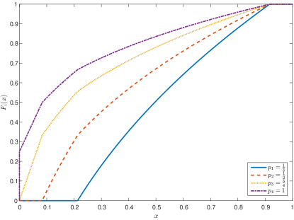
(a)

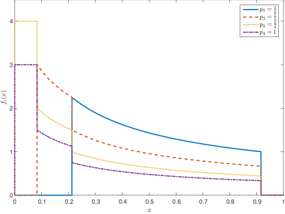
(b)

Figure 1: The CDFs (a) and the PDFs (b) when $p_{1}=\frac{1}{3}$, $p_{2}=\frac{1}{2}$, $p_{3}=\frac{3}{4}$ and $p_{4}=1$

A graphical illustration of the bidders’ CDFs (1a) and PDFs (1b) can be found in figure 1.

Proof of Theorem 7

Let $p_{1},\dots,p_{n}$ be the announced participation probabilities, and let $p^{\prime}_{r}<p_{r}$ be bidder $r$ real participation probability. For every $i\neq r$, bidder $i$’s expected profit from bid $x$ is:

$$\pi_{i}(x)=\left(p^{\prime}_{r}F_{r}(x)+1-p^{\prime}_{r}\right)\prod_{j=1;j\neq i,r}^{n}\left(p_{j}F_{j}(x)+1-p_{j}\right).$$

The values of this function change according to the relation between $r$, $i$ and $x$. The following lemmata offer some insights regarding the optimal strategy for a bidder.

Lemma 24.

Let $p_{1},\dots,p_{n}$ be the announced participation probabilities, and let $p^{\prime}_{r}<p_{r}$ be bidder $r$ real participation probability. For every $i>r$, the expected profit of bidder $i$ from bidding $x\in\left[\underline{s}_{k},\underline{s}_{k-1}\right)$, for $k\leq i$ and $k>r$, is:

$$\pi_{i}(x)=\frac{1-p^{\prime}_{r}}{1-p_{r}}\left(\lambda+x\right)-x=\frac{p_{r}-p^{\prime}_{r}}{1-p_{r}}\left(\lambda+x\right)+\lambda.$$

Proof.

The expected profit of bidder $i$ from bidding $x\in\left[\underline{s}_{k},\underline{s}_{k-1}\right)$, for $k\leq i$ and $k>r$, is:

$$\begin{array}[]{rl}\pi_{i}\left(x\right)=&\prod\limits_{j=1;j\neq i,r}^{n}\left(p_{j}F_{j}\left(x\right)+1-p_{j}\right)\left(p^{\prime}_{r}F_{r}\left(x\right)+1-p^{\prime}_{r}\right)-x\\ =&\prod\limits_{j=1;j\neq r}^{k-1}\left(p_{j}F_{j}\left(x\right)+1-p_{j}\right)\prod\limits_{j=1;j\neq i}^{n}\left(p_{j}F_{j}\left(x\right)+1-p_{j}\right)\left(p^{\prime}_{r}F_{r}\left(x\right)+1-p^{\prime}_{r}\right)-x\\ =&\prod\limits_{j=1;j\neq r}^{k-1}\left(1-p_{j}\right)\prod\limits_{j=1;j\neq i}^{n}\left(H_{k}\left(x\right)\right)\left(1-p^{\prime}_{r}\right)-x\\ =&\prod\limits_{j=1;j\neq r}^{k-1}\left(1-p_{j}\right)H_{k}\left(x\right)^{n-k}\left(1-p^{\prime}_{r}\right)-x\\ =&\prod\limits_{j=1;j\neq r}^{k-1}\left(1-p_{j}\right)\left(\frac{\lambda+x}{\prod_{j=0}^{k-1}\left(1-p_{j}\right)}\right)\left(1-p^{\prime}_{r}\right)-x\\ =&\frac{1-p^{\prime}_{r}}{1-p_{r}}\left(\lambda+x\right)-x\\ =&\left(\frac{p_{r}-p^{\prime}_{r}}{1-p_{r}}\right)\left(\lambda+x\right)+\lambda.\end{array}$$ (66)

∎

In this case, this is larger than $\lambda$, and grows with the bid, though the maximal bid (due to the fact that $k>r$) is $\underline{s}_{r}$.

When either $i<r$ or $i>r$, bidder can bid in the support of both bidders.

Lemma 25.

Let $p_{1},\dots,p_{n}$ be the announced participation probabilities, and let $p^{\prime}_{r}$ be bidder $r$ real participation probability. For every $i\neq r$, the expected profit of bidder $i$ from bidding $x\in\left[\underline{s}_{k},\underline{s}_{k-1}\right)$, such that $k\leq\min\{i,r\}$ is:

$$\pi_{i}(x)=\frac{p_{r}-p^{\prime}_{r}}{p_{r}}\left(\lambda+x\right)\left(\left(\frac{\prod_{j=1}^{k-1}\left(1-p_{j}\right)}{\lambda+x}\right)^{\frac{1}{n-k}}-1\right)+\lambda.$$

Proof.

The expected profit of bidder $i$ from bidding $x\in\left[\underline{s}_{k},\underline{s}_{k-1}\right)$, such that $k\leq\min\{i,r\}$ is:

$$\begin{array}[]{rl}\pi_{i}\left(x\right)=&\prod\limits_{j=1;j\neq i,r}^{n}\left(p_{j}F_{j}\left(x\right)+1-p_{j}\right)\left(p^{\prime}_{r}F_{r}\left(x\right)+1-p^{\prime}_{r}\right)-x\\ =&\prod\limits_{j=1}^{k-1}\left(p_{j}F_{j}\left(x\right)+1-p_{j}\right)\prod\limits_{j=k;j\neq i,r}^{n}\left(p_{j}F_{j}\left(x\right)+1-p_{j}\right)\left(p^{\prime}_{r}F_{r}\left(x\right)+1-p^{\prime}_{r}\right)-x\\ =&\prod\limits_{j=1}^{k-1}\left(1-p_{j}\right)\prod\limits_{j=k;j\neq i,r}^{n}\left(H_{k}\left(x\right)\right)\left(p^{\prime}_{r}F_{r}\left(x\right)+1-p^{\prime}_{r}\right)-x\\ =&\prod\limits_{j=1}^{k-1}\left(1-p_{j}\right)H_{k}\left(x\right)^{n-k-1}\left(p^{\prime}_{r}\frac{H_{k}\left(x\right)+p_{r}-1}{p_{r}}+1-p^{\prime}_{r}\right)-x\\ =&\prod\limits_{j=1}^{k-1}\left(1-p_{j}\right)H_{k}\left(x\right)^{n-k-1}\left(\frac{p^{\prime}_{r}}{p_{r}}H_{k}\left(x\right)+\frac{p_{r}-p^{\prime}_{r}}{p_{r}}\right)-x\\ =&\prod\limits_{j=1}^{k-1}\left(1-p_{j}\right)H_{k}\left(x\right)^{n-k}\frac{p^{\prime}_{r}}{p_{r}}+\prod\limits_{j=1}^{k-1}\left(1-p_{j}\right)H_{k}\left(x\right)^{n-k-1}\frac{p_{r}-p^{\prime}_{r}}{p_{r}}-x\\ =&\prod\limits_{j=1}^{k-1}\left(1-p_{j}\right)\left(\frac{\lambda+x}{\prod_{j=0}^{k-1}\left(1-p_{j}\right)}\right)\frac{p^{\prime}_{r}}{p_{r}}+\prod\limits_{j=1}^{k-1}\left(1-p_{j}\right)H_{k}\left(x\right)^{n-k-1}\frac{p_{r}-p^{\prime}_{r}}{p_{r}}-x\\ =&\frac{p^{\prime}_{r}}{p_{r}}\left(\lambda+x\right)+\prod\limits_{\begin{array}[]{c}j=1\end{array}}^{k-1}\left(1-p_{j}\right)\left(\frac{\lambda+x}{\prod_{j=0}^{k-1}\left(1-p_{j}\right)}\right)^{\frac{n-k-1}{n-k}}\frac{p_{r}-p^{\prime}_{r}}{p_{r}}-x\\ =&\frac{p^{\prime}_{r}}{p_{r}}\left(\lambda+x\right)+\prod\limits\limits_{\begin{array}[]{c}j=1\end{array}}^{k-1}\left(1-p_{j}\right)^{\frac{1}{n-k}}\left(\lambda+x\right)^{\frac{n-k-1}{n-k}}\frac{p_{r}-p^{\prime}_{r}}{p_{r}}-x\\ =&\left(\lambda+x\right)\left(\frac{p^{\prime}_{r}}{p_{r}}+\frac{p_{r}-p^{\prime}_{r}}{p_{r}}\left(\frac{\lambda+x}{\prod_{j=0}^{k-1}\left(1-p_{j}\right)}\right)^{\frac{-1}{n-k}}\right)-x\\ =&\left(\lambda+x\right)\frac{p_{r}-p^{\prime}_{r}}{p_{r}}\left(\left(\frac{\lambda+x}{\prod_{j=0}^{k-1}\left(1-p_{j}\right)}\right)^{\frac{-1}{n-k}}-1\right)+\lambda.\end{array}$$ (67)

∎

Since $x<\underline{s}_{k-1}$, this means that $\lambda+x<\left(1-p_{k-1}\right)^{n-k}\prod_{j=0}^{k-1}\left(1-p_{j}\right)$, hence $\left(\frac{\lambda+x}{\prod_{j=0}^{k-1}\left(1-p_{j}\right)}\right)^{\frac{-1}{n-k}}>1$; again, this is an increase over $\lambda$, the position without sabotaging.

Lemma 26.

Let $p_{1},\dots,p_{n}$ be the announced participation probabilities, and let $p^{\prime}_{r}<p_{r}$ be bidder $r$ real participation probability. For every $i\neq r$ and for every $x\in\left[0,\underline{s}_{i}\right)$, there exists $x^{\prime}\in\left[\underline{s}_{i},1-\lambda\right]$, such that $\pi_{i}\left(x\right)\leq\pi_{i}\left(x^{\prime}\right)$.

Proof.

When $i<r$, bidder $i$ can bid in bidder $r$’s support and not in its own support, i.e., bidder $i$ can bid $x\in\left[\underline{s}_{k},\underline{s}_{k-1}\right)$ for $k\leq r$ and $i<k$. We first note that bidder $i$ can bid $\underline{s}_{i}$ in its support with expected utility of:

$$\pi_{i}\left(\underline{s}_{i}\right)=\left(1-p_{i}\right)^{n-i-1}\prod_{j=0}^{i-1}\left(1-p_{j}\right)\frac{p_{r}-p^{\prime}_{r}}{p_{r}}p_{i}+\lambda.$$ (68)

When $x$ is in bidder $r$’s support and not in bidder $i$’s support:

$$\begin{array}[]{rl}\pi_{i}\left(x\right)=&\prod\limits_{j=1;j\neq i,r}^{n}\left(p_{j}F_{j}\left(x\right)+1-p_{j}\right)\left(p^{\prime}_{r}F_{r}\left(x\right)+1-p^{\prime}_{r}\right)-x\\ =&\prod\limits_{j=1;j\neq i}^{k-1}\left(p_{j}F_{j}\left(x\right)+1-p_{j}\right)\prod\limits_{j=k;j\neq r}^{n}\left(p_{j}F_{j}\left(x\right)+1-p_{j}\right)\left(p^{\prime}_{r}F_{r}\left(x\right)+1-p^{\prime}_{r}\right)-x\\ =&\prod\limits_{j=1;j\neq i}^{k-1}\left(1-p_{j}\right)\prod\limits_{j=k;j\neq r}^{n}\left(H_{k}\left(x\right)\right)\left(\frac{p^{\prime}_{r}}{p_{r}}\left(H_{k}\left(x\right)-1\right)+1\right)-x\\ =&\frac{\prod_{j=0}^{k-1}\left(1-p_{j}\right)}{1-p_{i}}H_{k}\left(x\right)^{n-k}\left(\frac{p^{\prime}_{r}}{p_{r}}\left(H_{k}\left(x\right)-1\right)+1\right)-x\\ =&\frac{\lambda+x}{1-p_{i}}\left(\frac{p^{\prime}_{r}}{p_{r}}\left(\frac{\lambda+x}{\prod_{j=0}^{k-1}\left(1-p_{j}\right)}\right)^{\frac{1}{n-k}}-\frac{p^{\prime}_{r}}{p_{r}}+1\right)-x\\ =&\frac{\lambda+x}{1-p_{i}}\left(\frac{p^{\prime}_{r}}{p_{r}}\left(\frac{\lambda+x}{\prod_{j=0}^{k-1}\left(1-p_{j}\right)}\right)^{\frac{1}{n-k}}-\frac{p^{\prime}_{r}}{p_{r}}+p_{i}\right)+\lambda.\end{array}$$ (69)

If $p_{i}\geq\frac{p^{\prime}_{r}}{p_{r}}$ then $\pi_{i}\left(x\right)$ monotonic grows with $x$, and maximized when $x=\underline{s}_{i}$; While if $p_{i}<\frac{p^{\prime}_{r}}{p_{r}}$, differentiating $\pi_{i}\left(x\right)$ twice with respect to $x$ gives:

$$\frac{\partial^{2}}{\partial x^{2}}\pi_{i}\left(x\right)=\frac{p^{\prime}_{r}}{p_{r}}\frac{1}{1-p_{i}}\left(1+\frac{1}{n-k}\right)\left(\frac{1}{n-k}\right)\left(\frac{\lambda+x}{\prod_{j=0}^{k-1}\left(1-p_{j}\right)}\right)^{\frac{1}{n-k}-1}\prod_{j=0}^{k-1}\left(1-p_{j}\right)^{\frac{-1}{n-k}},$$ (70)

that is, for every $x\in\left[\underline{s}_{k},\underline{s}_{k-1}\right)$: $\frac{\partial^{2}}{\partial x^{2}}\pi_{i}\left(x\right)\geq 0$, hence, the extremum is a minimum point and the utility maximized when either $x=\underline{s}_{k-1}$ or $x=\underline{s}_{k}$.

When bidding $\underline{s}_{k}$ the expected utility is:

$$\begin{array}[]{rl}\pi_{i}\left(\underline{s}_{k}\right)=&\frac{\prod_{j=0}^{k-1}\left(1-p_{j}\right)\left(1-p_{k}\right)^{n-k}}{1-p_{i}}\left(\frac{p^{\prime}_{r}}{p_{r}}\left(1-p_{k}\right)-\frac{p^{\prime}_{r}}{p_{r}}+p_{i}\right)+\lambda\\ =&\frac{\prod_{j=0}^{k-1}\left(1-p_{j}\right)\left(1-p_{k}\right)^{n-k}}{1-p_{i}}\left(p_{i}-\frac{p^{\prime}_{r}}{p_{r}}p_{k}\right)+\lambda.\end{array}$$ (71)

If $p_{i}-\frac{p^{\prime}_{r}}{p_{r}}p_{k}<0$ then $\pi_{i}\left(\underline{s}_{k}\right)<\lambda\leq\pi_{i}\left(\underline{s}_{i}\right)$.

Otherwise, if $p_{i}-\frac{p^{\prime}_{r}}{p_{r}}p_{k}\geq 0$, since $i<k$ it holds that $p_{i}\leq p_{k}$, and therefore $\prod_{j=0}^{k-1}\left(1-p_{j}\right)\left(1-p_{k}\right)^{n-k}\leq\prod_{j=0}^{i-1}\left(1-p_{j}\right)\left(1-p_{i}\right)^{n-i}$ and

$$\begin{array}[]{rl}\pi_{i}\left(\underline{s}_{k}\right)\leq&\frac{\prod_{j=0}^{i-1}\left(1-p_{j}\right)\left(1-p_{i}\right)^{n-i}}{1-p_{i}}\left(p_{i}-\frac{p^{\prime}_{r}}{p_{r}}p_{k}\right)+\lambda\\ =&\prod_{j=0}^{i-1}\left(1-p_{j}\right)\left(1-p_{i}\right)^{n-i-1}\left(p_{i}-\frac{p^{\prime}_{r}}{p_{r}}p_{k}\right)+\lambda\\ \leq&\prod_{j=0}^{i-1}\left(1-p_{j}\right)\left(1-p_{i}\right)^{n-i-1}\left(p_{i}-\frac{p^{\prime}_{r}}{p_{r}}p_{i}\right)+\lambda\\ =&\prod_{j=0}^{i-1}\left(1-p_{j}\right)\left(1-p_{i}\right)^{n-i-1}\frac{p_{r}-p^{\prime}_{r}}{p_{r}}p_{i}+\lambda\\ =&\pi_{i}\left(\underline{s}_{i}\right).\end{array}$$ (72)

Similarly, $\pi_{i}\left(\underline{s}_{k-1}\right)\leq\pi_{i}\left(\underline{s}_{i}\right)$. That is, for every $x\in\left[\underline{s}_{k},\underline{s}_{k-1}\right)$: $\pi_{i}\left(x\right)\leq\pi_{i}\left(\underline{s}_{i}\right)$. Therefore, bidder $i$ has no incentive to bid outside of its support and in bidder $r$’s support.

When $x$ is outside of the support of both bidders, i.e. $x\in\left[\underline{s}_{k},\underline{s}_{k-1}\right)$ for $k>i$ and $k>r$:

$$\begin{array}[]{rl}\pi_{i}\left(x\right)=&\prod\limits_{j=1;j\neq i,r}^{n}\left(p_{j}F_{j}\left(x\right)+1-p_{j}\right)\left(p^{\prime}_{r}F_{r}\left(x\right)+1-p^{\prime}_{r}\right)-x\\ =&\prod\limits_{j=1;j\neq i,r}^{k-1}\left(p_{j}F_{j}\left(x\right)+1-p_{j}\right)\prod\limits_{j=k}^{n}\left(p_{j}F_{j}\left(x\right)+1-p_{j}\right)\left(p^{\prime}_{r}F_{r}\left(x\right)+1-p^{\prime}_{r}\right)-x\\ =&\prod\limits_{j=1;j\neq i,r}^{k-1}\left(1-p_{j}\right)\prod\limits_{j=k}^{n}\left(H_{k}\left(x\right)\right)\left(1-p^{\prime}_{r}\right)-x\\ =&\frac{\prod_{j=0}^{k-1}\left(1-p_{j}\right)}{1-p_{i}}H_{k}\left(x\right)^{n-k+1}\frac{1-p^{\prime}_{r}}{1-p_{r}}-x\\ =&\frac{\prod_{j=0}^{k-1}\left(1-p_{j}\right)}{1-p_{i}}\frac{1-p^{\prime}_{r}}{1-p_{r}}\left(\frac{\lambda+x}{\prod_{j=0}^{k-1}\left(1-p_{j}\right)}\right)^{\frac{n-k+1}{n-k}}-x\\ =&\frac{\prod_{j=0}^{k-1}\left(1-p_{j}\right)^{\frac{-1}{n-k}}}{1-p_{i}}\frac{1-p^{\prime}_{r}}{1-p_{r}}\left(\lambda+x\right)^{\frac{n-k+1}{n-k}}-x\\ =&\left(\lambda+x\right)\left(\frac{1-p^{\prime}_{r}}{\left(1-p_{i}\right)\left(1-p_{r}\right)}\left(\frac{\lambda+x}{\prod_{j=0}^{k-1}\left(1-p_{j}\right)}\right)^{\frac{1}{n-k}}-1\right)+\lambda.\end{array}$$ (73)

Differentiating the above twice with respect to $x$ gives:

$$\frac{\partial^{2}}{\partial x^{2}}\pi_{i}\left(x\right)=\frac{1-p^{\prime}_{r}}{\left(1-p_{i}\right)\left(1-p_{r}\right)}\left(1-\frac{1}{n-k}\right)\frac{1}{n-k}\left(\frac{\lambda+x}{\prod_{j=0}^{k-1}\left(1-p_{j}\right)}\right)^{\frac{1}{n-k}-1}\prod_{j=0}^{k-1}\left(1-p_{j}\right)^{\frac{-1}{n-k}}.$$ (74)

Again, for every $x\in\left[\underline{s}_{k},\underline{s}_{k-1}\right)$: $\frac{\partial^{2}}{\partial x^{2}}\pi_{i}\left(x\right)\geq 0$, hence, the extremum is a minimum point and the utility maximized when either $x=\underline{s}_{k-1}$ or $x=\underline{s}_{k}$.

When bidding $\underline{s}_{k}$ the expected utility is:

$$\begin{array}[]{rl}\pi_{i}\left(\underline{s}_{k}\right)=&\left(1-p_{k}\right)^{n-k}\left(\frac{1-p^{\prime}_{r}}{\left(1-p_{i}\right)\left(1-p_{r}\right)}\left(\frac{\left(1-p_{k}\right)^{n-k}\prod_{j=0}^{k-1}\left(1-p_{j}\right)}{\prod_{j=0}^{k-1}\left(1-p_{j}\right)}\right)^{\frac{1}{n-k}}-1\right)\prod_{j=0}^{k-1}\left(1-p_{j}\right)+\lambda\\ =&\left(1-p_{k}\right)^{n-k}\left(\frac{1-p^{\prime}_{r}}{\left(1-p_{i}\right)\left(1-p_{r}\right)}\left(1-p_{k}\right)-1\right)\prod_{j=0}^{k-1}\left(1-p_{j}\right)+\lambda.\end{array}$$ (75)

If $\frac{1-p^{\prime}_{r}}{\left(1-p_{i}\right)\left(1-p_{r}\right)}\left(1-p_{k}\right)-1\leq 0$, then $\pi_{i}\left(\underline{s}_{k}\right)\leq\lambda\leq\pi_{i}\left(\underline{s}_{r}\right)$.

Otherwise, $\frac{1-p^{\prime}_{r}}{\left(1-p_{i}\right)\left(1-p_{r}\right)}\left(1-p_{k}\right)-1>0$. In this case we separate the two sub-cases; if $r<i$, the expected utility for bidder $i$ from bidding $\underline{s}_{r}$ in its support is:

$$\pi_{i}\left(\underline{s}_{r}\right)=\left(p_{r}-p^{\prime}_{r}\right)\left(1-p_{r}\right)^{n-r-1}\prod_{j=0}^{r-1}\left(1-p_{j}\right)+\lambda$$ (76)

since $k>i$ we have that $\frac{1-p_{k}}{1-p_{i}}\leq 1$ and since $k>r$ we have that
$\prod_{j=0}^{k-1}\left(1-p_{j}\right)\left(1-p_{k}\right)^{n-k}\leq\prod_{j=0}^{r-1}\left(1-p_{j}\right)\left(1-p_{r}\right)^{n-r}$, hence–

$$\begin{array}[]{rl}\pi_{i}\left(\underline{s}_{k}\right)=&\left(\frac{1-p^{\prime}_{r}}{\left(1-p_{i}\right)\left(1-p_{r}\right)}\left(1-p_{k}\right)-1\right)\left(1-p_{k}\right)^{n-k}\prod_{j=0}^{k-1}\left(1-p_{j}\right)+\lambda\\ \leq&\left(\frac{1-p^{\prime}_{r}}{1-p_{r}}-1\right)\left(1-p_{k}\right)^{n-k}\prod_{j=0}^{k-1}\left(1-p_{j}\right)+\lambda\\ \leq&\left(\frac{1-p^{\prime}_{r}}{1-p_{r}}-1\right)\left(1-p_{k}\right)^{n-r}\prod_{j=0}^{r-1}\left(1-p_{j}\right)+\lambda\\ \leq&\left(\frac{1-p^{\prime}_{r}}{1-p_{r}}-1\right)\left(1-p_{r}\right)^{n-r}\prod_{j=0}^{r-1}\left(1-p_{j}\right)+\lambda\\ =&\frac{p_{r}-p^{\prime}_{r}}{1-p_{r}}\left(1-p_{r}\right)^{n-r}\prod_{j=0}^{r-1}\left(1-p_{j}\right)+\lambda\\ =&\left(p_{r}-p^{\prime}_{r}\right)\left(1-p_{r}\right)^{n-r-1}\prod_{j=0}^{r-1}\left(1-p_{j}\right)+\lambda\\ =&\pi_{i}\left(\underline{s}_{r}\right).\end{array}$$ (77)

Similarly $\pi_{i}\left(\underline{s}_{k-1}\right)\leq\pi_{i}\left(\underline{s}_{r}\right)$, that is, for every $x\in\left[\underline{s}_{k},\underline{s}_{k-1}\right)$: $\pi_{i}\left(x\right)\leq\pi_{i}\left(\underline{s}_{r}\right)$. And in a similar way if $r>i$, for every $k>r$, it holds that both $\pi_{i}\left(\underline{s}_{k}\right)\leq\pi_{i}\left(\underline{s}_{i}\right)$ and $\pi_{i}\left(\underline{s}_{k-1}\right)\leq\pi_{i}\left(\underline{s}_{i}\right)$, thus for every $x\in\left[\underline{s}_{k},\underline{s}_{k-1}\right)$: $\pi_{i}\left(x\right)\leq\pi_{i}\left(\underline{s}_{i}\right)$. Therefore, even if bidder $i$ sabotaged bidder $r$, bidder $i$ has no incentive to deviate from its support. ∎

Armed with Lemmata 24, 25 and 26 we may proceed to prove Theorem 7.

Theorem 7.

Let $p_{1},\dots,p_{n}$ be the announced participation probabilities, and let $p^{\prime}_{r}<p_{r}$ be bidder $r$ real participation probability. For every $i\neq r$, Algorithm 1 finds the optimal bid for bidder $i$.

Proof.

Lemmata 24, 25 and 26 tell us that the optimal bid is in $\left[\underline{s}_{\min\{i,r\}},\underline{s}_{0}\right]$.

Now, in order find the optimal bid in $\left[\underline{s}_{k},\underline{s}_{k-1}\right]$ for $k\leq\min\{i,r\}$, we differentiate $\pi_{i}$ with respect to $x$:

$$\frac{\partial}{\partial x}\pi_{i}\left(x\right)=\frac{p_{r}-p^{\prime}_{r}}{p_{r}}\left(1-\frac{1}{n-k}\right)\left(\frac{\lambda+x}{\prod_{j=1}^{k-1}\left(1-p_{j}\right)}\right)^{\frac{-1}{n-k}}-\frac{p_{r}-p^{\prime}_{r}}{p_{r}}.$$ (78)

That is, $\pi_{i}\left(x\right)$ maximized when

$$x=\left(1-\frac{1}{n-k}\right)^{n-k}\prod_{j=1}^{k-1}\left(1-p_{j}\right)-\lambda.$$ (79)

Now, $x\in\left[\underline{s}_{k},\underline{s}_{k-1}\right]$, and it holds that

$$\begin{array}[]{cc}\left(1-\frac{1}{n-k}\right)^{n-k}\prod_{j=1}^{k-1}\left(1-p_{j}\right)-\lambda\in\left[\underline{s}_{k},\underline{s}_{k-1}\right]&\iff\\ \frac{1}{n-k}\in\left[p_{k-1},p_{k}\right].\end{array}$$ (80)

Thus, the optimal bid for bidder $i$ in $\left[\underline{s}_{k},\underline{s}_{k-1}\right]$, depends if either $\frac{1}{n-k}\in\left[p_{k-1},p_{k}\right]$, $\frac{1}{n-k}<p_{k-1}$ or $\frac{1}{n-k}>p_{k}$.

• If $\frac{1}{n-k}\in\left[p_{k-1},p_{k}\right]$ then the optimal bid in $\left[\underline{s}_{k},\underline{s}_{k-1}\right]$ is

  $$x=\left(1-\frac{1}{n-k}\right)^{n-k}\prod_{j=1}^{k-1}\left(1-p_{j}\right)-\lambda$$

  and the expected profit is:

  $$\frac{1}{n-k}\left(1-\frac{1}{n-k}\right)^{n-k-1}\prod_{j=1}^{k-1}\left(1-p_{j}\right)\frac{p_{r}-p^{\prime}_{r}}{p_{r}}+\lambda.$$ (81)

• If $\frac{1}{n-k}<p_{k-1}$ then the optimal bid in $\left[\underline{s}_{k},\underline{s}_{k-1}\right]$ is $x=\underline{s}_{k-1}$ and the expected profit is:

  $$p_{k-1}\left(1-p_{k-1}\right)^{n-k-1}\prod_{j=1}^{k-1}\left(1-p_{j}\right)\frac{p_{r}-p^{\prime}_{r}}{p_{r}}+\lambda.$$ (82)

• If $\frac{1}{n-k}>p_{k}$ then the optimal bid in $\left[\underline{s}_{k},\underline{s}_{k-1}\right]$ is $x=\underline{s}_{k}$ and the expected profit is:

  $$p_{k}\left(1-p_{k}\right)^{n-k-1}\prod_{j=1}^{k-1}\left(1-p_{j}\right)\frac{p_{r}-p^{\prime}_{r}}{p_{r}}+\lambda.$$ (83)

Now, for every $k\leq\min\{i,r\}$ let $x_{i,k}$ be the optimal bid in $\left[\underline{s}_{k},\underline{s}_{k-1}\right]$, let $\pi_{i,k}=\pi_{i}\left(x_{i,k}\right)$ and let $j\in\arg\max_{k}\pi_{i,k}$. As $x_{i,k}$ is the optima bid in $\left[\underline{s}_{k},\underline{s}_{k-1}\right]$, it follows that $x_{i,j}$ is the optima bid in $\left[\underline{s}_{\min\{i,r\}},\underline{s}_{0}\right]$. ∎

Proof of Theorem 8

Theorem 8.

The expected bid of every bidder is:

$$\mathbb{E}\left[bid\right]=\frac{1}{np}\left(1-\lambda\left(1+p\left(n-1\right)\right)\right)$$ (84)

and the variance of the bid is:

$$\mathrm{Var}\left[bid\right]=\frac{1-(1-p)^{2n-1}}{(2n-1)p}-\frac{\left(1-(1-p)^{n}\right)^{2}}{n^{2}p^{2}}.$$ (85)

The expected bid and the variance are neither monotonic in $n$ nor in $p$.

Proof.

As this case is a particular instance of the general case presented above, we can characterize the CDF for every bidder —

$$F_{n,p}\left(x\right)=\begin{cases}1&x>1-\lambda\\ \frac{\left(\lambda+x\right)^{\frac{1}{n-1}}+p-1}{p}\,\,&x\in\left[0,1-\lambda\right]\\ 0&x<0\end{cases}$$ (86)

where $\lambda=\left(1-p\right)^{n-1}$, which implies that the bidders’ PDF is:

$$f_{n,p}\left(x\right)=\frac{\mathrm{d}}{\mathrm{d}x}F_{n,p}\left(x\right)=\begin{cases}0&x>1-\lambda\\ \frac{\left(\lambda+x\right)^{\frac{2-n}{n-1}}}{p\left(n-1\right)}\,\,&x\in\left[0,1-\lambda\right]\\ 0&x<0\end{cases}.$$ (87)

The expected bid of every bidder is:

$$\begin{array}[]{rl}\mathbb{E}\left[bid\right]=&\int_{0}^{1-\lambda}xf_{n,p}\left(x\right)\,\mathrm{d}x\\ =&\frac{1}{np}\left(1-\lambda\left(1+p\left(n-1\right)\right)\right)\end{array}$$ (88)

which is neither monotonic in $n$ nor in $p$.

The bid squared, in expectation, is:

$$\begin{array}[]{rl}\mathbb{E}\left[bid^{2}\right]=&\int_{0}^{1-\lambda}x^{2}f_{n,p}\left(x\right)\,\mathrm{d}x\\ =&\left.\left(\frac{\left(\lambda+x\right)^{\frac{1}{n-1}}\lambda^{2}}{p}-2\frac{\left(\lambda+x\right)^{\frac{n}{n-1}}\lambda}{np}+\frac{\left(\lambda+x\right)^{\frac{2n-1}{n-1}}}{\left(2n-1\right)p}\right)\right|_{0}^{1-\lambda}\\ =&\frac{1}{p}\left(\frac{1}{2n-1}-\frac{2}{n}\left(1-p\right)^{n-1}+\left(1-p\right)^{2n-2}-\left(1-p\right)^{2n-1}\frac{2\left(n-1\right)^{2}}{n\left(2n-1\right)}\right)\end{array}$$ (89)

hence,

$$\begin{array}[]{rl}Var\left(bid\right)=&\mathbb{E}\left[bid^{2}\right]-\mathbb{E}^{2}\left[bid\right]\\ =&\frac{1}{p}\left(\frac{1}{\left(2n-1\right)}-\frac{2}{n}\left(1-p\right)^{n-1}+\left(1-p\right)^{2n-2}-\left(1-p\right)^{2n-1}\frac{2\left(n-1\right)^{2}}{n\left(2n-1\right)}\right)\\ &-\left(\frac{1}{np}\left(1-\left(1-p\right)^{n-1}\left(1+p\left(n-1\right)\right)\right)\right)^{2}\\ =&\frac{1-(1-p)^{2n-1}}{(2n-1)p}-\frac{\left(1-(1-p)^{n}\right)^{2}}{n^{2}p^{2}}\end{array}$$ (90)

which is, again, neither monotonic in $n$ nor in $p$. ∎

Proof of Theorem 9

Theorem 9.

The variance of the bidder profit is:

$$\mathrm{Var}\left[BP\right]=\frac{n-1}{n\left(2n-1\right)}-\frac{\left(1-p\right)^{n}}{n}+\left(p+\frac{1}{2n-1}\right)\left(1-p\right)^{2n-1}.$$

And the variance is monotonic increasing in $p$.

Proof.

The squared of the bidder profit is:

$$\begin{array}[]{rl}\mathbb{E}\left[BP^{2}\right]=&\int_{\lambda-1}^{0}z^{2}g_{BP}\left(z\right)\,\partial z+\int_{\lambda}^{1}z^{2}g_{BP}\left(z\right)\,\mathrm{d}z\\ =&\int_{\lambda-1}^{0}z^{2}\frac{\left(\lambda-z\right)^{\frac{2-n}{n-1}}}{n-1}\left(1-\left(\lambda-z\right)\right)\,\partial z+\int_{\lambda}^{1}z^{2}\frac{\left(\lambda+1-z\right)^{\frac{1}{n-1}}}{n-1}\,\mathrm{d}z\\ =&\left.\left(\lambda-z\right)^{\frac{1}{n-1}}\left(\frac{\lambda(\lambda+2)\left(\lambda-z\right)}{n}+\frac{\left(\lambda-z\right)^{3}}{3n-2}-\lambda^{2}-\frac{(2\lambda+1)\left(\lambda-z\right)^{2}}{2n-1}\right)\right|_{\lambda-1}^{0}\\ &\left.+\left(\lambda-z\right)^{\frac{1}{n-1}}\left(\left(\lambda+1-z\right)\left(\frac{2\lambda+2}{2n-1}-\frac{\lambda+1-z}{3n-2}\right)-\frac{(\lambda+1)^{2}}{n}\right)\right|_{\lambda}^{1}\\ =&\left(\lambda-z\right)^{\frac{1}{n-1}}\left(\frac{2\lambda\left(n-1\right)^{2}}{n\left(3n-2\right)\left(2n-1\right)}-\frac{2\left(n-1\right)^{2}}{n\left(2n-1\right)}\right)+\lambda^{2}\frac{n-1}{n}-\lambda\frac{2\left(n-1\right)}{n\left(2n-1\right)}+\frac{n-1}{\left(3n-2\right)\left(2n-1\right)}\\ &-\left(1-p\right)^{n}\left(\frac{2\lambda^{2}\left(n-1\right)^{2}}{n\left(3n-2\right)\left(2n-1\right)}+\frac{2\lambda\left(n-1\right)}{n\left(2n-1\right)}+\frac{1}{n}\right)\\ &+\frac{\lambda^{2}}{n}+\frac{2\lambda\left(n-1\right)}{n\left(2n-1\right)}+\frac{2\left(n-1\right)^{2}}{n\left(3n-2\right)\left(2n-1\right)}\\ =&\frac{n-1}{n\left(2n-1\right)}-\frac{\left(1-p\right)^{n}}{n}+\left(1-p\right)^{2n-2}-\frac{2\left(n-1\right)}{2n-1}\left(1-p\right)^{2n-1}.\end{array}$$ (91)

Hence the variance of the profit of every bidder is:

$$\begin{array}[]{rl}\mathrm{Var}\left[BP\right]=&\mathbb{E}\left[BP^{2}\right]-\mathbb{E}^{2}\left[BP\right]\\ =&\frac{n-1}{n\left(2n-1\right)}-\frac{\left(1-p\right)^{n}}{n}+\left(p+\frac{1}{2n-1}\right)\left(1-p\right)^{2n-1}\end{array}$$ (92)

Differentiating the above with respect to $p$ gives:

$$\frac{\partial}{\partial p}Var\left(BP\right)=(1-p)^{n-1}-2n\cdot p\left(1-p\right)^{2n-2}.$$ (93)

Now,

$$\begin{array}[]{rlc}\frac{\partial}{\partial p}\mathrm{Var}\left[BP\right]&\geq 0&\iff\\ (1-p)^{n-1}-2n\cdot p\left(1-p\right)^{2n-2}&\geq 0&\iff\\ p\left(1-p\right)^{n-1}&\leq\frac{1}{2n}\end{array}$$ (94)

since $p\left(1-p\right)^{n-1}$ maximized when $p=\frac{1}{n}$,

$$\begin{array}[]{rlc}\frac{\partial}{\partial p}\mathrm{Var}\left[BP\right]&\geq 0&\iff\\ \left(1-\frac{1}{n}\right)^{n-1}&\leq\frac{1}{2}\end{array}$$ (95)

which holds for every $n\geq 2$. Therefore for every $n\geq 2$ the variance of the bidder profit increases with $p$.

∎

Proof of Theorem 29

Theorem 29.

The variance of the auctioneer in the max profit model is:

$$\begin{array}[]{rl}\mathrm{Var}\left[AP\right]=&\left(1-p\right)^{2n-2}-\frac{2n\left(1-p\right)^{n-1}}{2n-1}+\frac{n}{3n-2}-\frac{2\left(n-1\right)^{2}\left(1-p\right)^{3n-2}}{\left(3n-2\right)\left(2n-1\right)}\\ &-\left(\frac{n}{2n-1}+\frac{n-1}{2n-1}\left(1-p\right)^{2n-1}-\left(1-p\right)^{n-1}\right)^{2}.\end{array}$$ (96)

Proof.

The profit squared, in expectation, is:

$$\begin{array}[]{rl}\mathbb{E}\left[AP^{2}\right]=&\int_{0}^{1-\lambda}x^{2}\cdot\frac{n}{n-1}\left(\lambda+x\right)^{\frac{1}{n-1}}\,\mathrm{d}x\\ =&\left.\left(\lambda+x\right)^{\frac{n}{n-1}}\left(\lambda^{2}-\lambda\frac{2n\left(\lambda+x\right)}{2n-1}+\frac{n\left(\lambda+x\right)^{2}}{3n-2}\right)\right|_{0}^{1-\lambda}\\ =&\left(1-p\right)^{2n-2}-\frac{2n\left(1-p\right)^{n-1}}{2n-1}+\frac{n}{3n-2}-\frac{2\left(n-1\right)^{2}\left(1-p\right)^{3n-2}}{\left(3n-2\right)\left(2n-1\right)}.\end{array}$$ (97)

Hence, the variance is:

$$\begin{array}[]{rl}\mathrm{Var}\left[AP\right]=&\left(1-p\right)^{2n-2}-\frac{2n\left(1-p\right)^{n-1}}{2n-1}+\frac{n}{3n-2}-\frac{2\left(n-1\right)^{2}\left(1-p\right)^{3n-2}}{\left(3n-2\right)\left(2n-1\right)}\\ &-\left(\frac{n}{2n-1}+\frac{n-1}{2n-1}\left(1-p\right)^{2n-1}-\left(1-p\right)^{n-1}\right)^{2}.\end{array}$$ (98)

∎

References

- Bachrach et al. [2011] Yoram Bachrach, Reshef Meir, Michal Feldman, and Moshe Tennenholtz. Solving cooperative reliability games. In Proceedings of the 28th Conference in Uncertainty in Artificial Intelligence (UAI), pages 27–34, Barcelona, Spain, July 2011.
- Bachrach et al. [2014] Yoram Bachrach, Rahul Savani, and Nisarg Shah. Cooperative max games and agent failures. In Proceedings of the 13th International Joint Conference on Autonomous Agents and Multiagent Systems (AAMAS), pages 29–36, Paris, France, May 2014.
- Baye et al. [1996] Michael R. Baye, Dan Kovenock, and Casper G. Vries. The all-pay auction with complete information. Economic Theory, 8(2):291–305, 1996. ISSN 1432-0479.
- Chawla et al. [2012] Shuchi Chawla, Jason D. Hartline, and Balasubramanian Sivan. Optimal crowdsourcing contests. In Proceedings of the 23rd Annual ACM-SIAM Symposium on Discrete Algorithms (SODA), pages 856–868, Kyoto, Japan, 2012. SIAM.
- DiPalantino and Vojnović [2009] Dominic DiPalantino and Milan Vojnović. Crowdsourcing and all-pay auctions. In Proceedings of the 10th ACM conference on Electronic commerce, pages 119–128, Stanford, California, July 2009.
- Dyer et al. [1989] Douglas Dyer, John H. Kagel, and Dan Levin. Resolving uncertainty about the number of bidders in independent private-value auctions: An experimental analysis. The RAND Journal of Economics, 20(2):268–279, 1989.
- Hillman and Riley [1989] Arye L. Hillman and John G. Riley. Politically contestable rents and transfers. Economics & Politics, 1(1):17–39, March 1989.
- Lev et al. [2013] Omer Lev, Maria Polukarov, Yoram Bachrach, and Jeffrey S. Rosenschein. Mergers and collusion in all-pay auctions and crowdsourcing contests. In Proceedings of the 12th International Coference on Autonomous Agents and Multiagent Systems (AAMAS), pages 675–682, St. Paul, Minnesota, May 2013.
- Lu and Yang [2003] Dennis Lu and Jing Yang. Auction participation and market uncertainty: Evidence from canadian treasury auctions. In Conference paper presented at the Canadian Economics Association 37th Annual Meeting, 2003.
- Maskin and Riley [2003] Eric Maskin and John Riley. Uniqueness of equilibrium in sealed high-bid auctions. Games and Economic Behavior, 45(2):395–409, November 2003.
- Matthews [1987] Steven Matthews. Comparing auctions for risk averse buyers: A buyer’s point of view. Econometrica, 55(3):633–646, May 1987.
- McAfee and McMillan [1987] Randolph Preston McAfee and John McMillan. Auctions with a stochastic number of bidders. Journal of Economic Theory, 43(1):1–19, October 1987.
- Meir et al. [2012] Reshef Meir, Moshe Tennenholtz, Yoram Bachrach, and Peter Key. Congestion games with agent failures. In Proceedings of the 26th National Conference on Artificial Intelligence (AAAI), pages 1401–1407, Toronto, Canada, July 2012.
- Menezes and Monteiro [2000] Flavio M. Menezes and Paulo K. Monteiro. Auctions with endogenous participation. Review of Economic Design, 5(1):71–89, March 2000.