Real space renormalization group for Ising Spin Glass and other glassy models.
I. Disordered Ising model. General formalism

Abstract

Here is the first part of the summary of my work on random Ising model using real-space renormalization group (RSRG), also known as a Migdal-Kadanoff one. This approximate renormalization scheme was applied to the analysis thermodynamic properties of the model, and of probabilistic properties of a pair correlator, which is a fluctuating object in disordered systems.

I Introduction

The main goal of this series of publications is to introduce and apply a new theoretical method aimed at the description of the wide class of statistical phenomena known under the name ”spin glasses” (ea75, ). The name originates from the specific class of disordered magnetics with elementary dipoles (spins) being frozen in random orientations. It appeared, however, that similar phenomena are widespread in Nature. Numerous phenomena in physics (amorphous magnetism and ferroelectricity, structural glasses), biology (patterns formation in neural networks, proteins folding), and computer science (storage and interaction of patterns in memory) may be described using a mathematical models of the same class. Numerous books and reviews on the subject are available (see (mpv87, ; by86, ; vsd93, ; fh93, ; cc05, ; fz10, ; alg13, ; hn01, ) and references cited therein).

Among all the models, describing glassy behavior, the simplest is the disordered Ising model with competing interactions. Originally it was introduced to describe glassy state of a solution of a magnetic metal in a nonmagnetic one, e.g. iron in gold. There the point is the exchange interaction between magnetic ions may be either ferro- or antiferromagnetic, depending upon the distance between ions, which is a fluctuating random variable. The specific feature of such a system is the possibility of frustrations in it. A primitive illustration may looks like this: Let us consider three Ising spins, $\sigma_{1,2,3}=\pm 1$. The Hamiltonian is:

$${\cal H}=-J_{12}\sigma_{1}\sigma_{2}-J_{23}\sigma_{2}\sigma_{3}-J_{31}\sigma_{3}\sigma_{1}\,.$$

If all the pair interaction energies $J_{ij}>0$ (purely ferromagnetic case), then the ground state is two-fold degenerate, either all spins are $+1$, or $-1$. However, if one or all three interactions are negative, then the specific case becomes possible. For example, let us set $J_{12}=J_{23}=J>0,\,J_{31}=-J$. Spin configurations $\left(+++\right)$, $\left(-++\right)$ and $\left(++-\right)$ have the energy, equal to $-J$, while the configuration $\left(+-+\right)$ has the energy $+3J$. The ground state becomes six-fold degenerate. The situation is quite similar if $J_{12}=J_{23}=J_{31}=-J<0$. This reasoning can be easily generalized to the case, when $N$ Ising spins are arranged in a ring, and the number of antiferromagnetic interactions is odd. The special attention should be paid to the fact, that, strictly speaking, this degeneracy exists only if all the interaction energies are equal in value, $\left|J_{ij}\right|=J$. For example, if in the triangle we have: $J_{12}=J_{23}=J$, $J_{31}=-\tilde{J}$, and $J>\tilde{J}>0$, the ground state is ferromagnetic and only two-fold degenerate. If to assume $J_{ij}$ to be fluctuating random variables, then, in a common case, the measure of frustrated configurations is zero.

If there is a macroscopic number of frustrations in a macroscopic system of a size $N\to\infty$, then the degeneracy of the ground state appears to be $\sim a^{N}$, $a\gtrsim 1$. This leads to a nonzero value of the entropy in the thermodynamic limit (fss13, ). The example is the antiferromagnetic Ising model on the triangular lattice. However, in a disordered systems frustrations, strictly speaking, exist only if the distribution of couplings is something very special, e.g. $p\left(J_{ij}\right)=c\delta\left(J_{ij}-J\right)+\left(1-c\right)\delta\left(J_{ij}+J\right)$. Usually, some configurations close to frustration may be realized, rather then true frustration, if ferro- and antiferromagnetic interactions coexist in a system. Therefore, one can expect the residual entropy to be zero, but some kind of singularity of the entropy and of the specific heat at zero temperature is possible.

Originally the Migdal-Kadanoff real space renormalization group (RSRG) was introduced more then fifty years ago by Leo Kadanoff (lpk66, ). Then its continuous rescaling version was introduced by A.A. Migdal (aam75, ). Comprehensive review of further developments of the RSRG approach was recently given in (ewkk14, ).

The first attempt to apply RSRG to spin glass problem was made by Droz and Matasinas (dm80, ). However, there severe and unjustified approximations were made for the problem to be solvable. Then the RSRG with integer rescaling factor was used in a number of works (see e.g. (th96, ; ncnc99, ; mbd98, ; mprz99, ; sn09, )) The RSRG analysis was applied in (onm08, ) to analyze the multicritical points (coexistence of (para/ferro)magnetic and spin glass phases) positions. A different version of RSRG for spin glasses was used in (cp11, ; mc11, ). Tensor RSRG for spin glasses was used in (wqz14, ), and RSRG for Ising model with long range coupling was elaborated in (cm16, )

A functional version of RSRG with continuous rescaling was introduced in (spjw98, ) to study the behavior of conductivity at and near the percolation threshold. Actually the RSRG is exact for one-dimensional systems with short-range interaction, so it was applied for $\left((1+\epsilon\right)$-dimensional fractals.It was a surprise, that renormalization equations (nonlinear integro-differential ones) there allow exact solution, provided by the saddle point approximation in the integrals.

This paper, first in a series, is devoted to the construction of mathematical formalism of RSRG for a disordered Ising model. In Section II general concepts of the statistical mechanics of disordered systems was applied to the Ising model. The crucial point is to perform configuration average of the free energy. Here a new representation of the distribution of interaction energies is introduced and named ${\cal T}$-representation. Formulas, connecting ${\cal T}$-representation with Fourier (or two-sided Laplace) one are derived. Averaged free energy is defined as a functional of the distribution of interaction energies. Adding one extra link, not necessary between nearest neighbors, and calculating the corresponding variation of the free energy as a function of the strength the length of this link provide us with generating function for the momenta of the spin-spin correlator, — this is a straightforward generalization of the approach elaborated by A.N. Vasil’ev (anv98, ).

In Section III RSRG for a disordered Ising model is formulated, first in Subsection III.1 — for a hierarchical graph. Here the rescaling factor is integer. In Subsection III.2 the transition to infinitesimal rescaling is considered. In Subsection III.3 explicit expressions for thermodynamic quantities are given. The Section IV contains brief summary of results. Finally, in the last Section V some preliminary results of the next paper are adduced. Technical details are taken into two Appendices.

II Statistical mechanics of the disordered Ising model.

II.1 The Ising model.

II.1.1 Definitions.

The Ising model consists of $N$ binary variables (“spins”) $\sigma_{i}$, $i=1,2,\dots N$, that can be in one of two states, $\sigma_{i}=\pm 1$, or “spin up/down”. These spins are either placed randomly in a D-dimensional space, or arranged in a graph, usually a D-dimensional lattice. The Hamiltonian of the model is:

$$\mathcal{H}\left(\left\{\sigma_{i}\right\}\right)=-\sum_{i=1}^{N}h_{i}\sigma_{i}-\frac{1}{2}\sum_{i,j=1}^{N}J_{ij}\sigma_{i}\sigma_{j}.$$ (1)

Here $h_{i}$ are local magnetic fields. Here I will assume $h_{i}=0$. $J_{ij}=J\left(\mathbf{r}_{i}-\mathbf{r}_{j}\right)$ are pair interaction energies. They may be either ferromagnetic (FM), $J_{ij}>0$, or antiferromagnetic (AFM), $J_{ij}<0$, which favors two spins in the pair to be either aligned, $\sigma_{i}=\sigma_{j}$, or anti-aligned, $\sigma_{i}=-\sigma_{j}$.

The partition function of the model is:

$$Z_{N}\left(\left\{K_{ij}\right\}\right)=\sum_{\left\{\sigma_{i}=\pm 1\right\}}\exp\left(\frac{1}{2}\sum_{i,j}^{N}K_{ij}\sigma_{i}\sigma_{j}\right)\,.$$ (2)

Here $K_{ij}=J_{ij}/T$ are the reduced coupling energies ($T$ is the temperature in the energy units). The free energy $\mathcal{F}$ of the system is:

$$\mathcal{F}_{N}\left(\left\{K_{ij}\right\}\right)=-T\ln Z_{N}\left(\left\{K_{ij}\right\}\right)\,.$$ (3)

The pair correlator is defined as:

$$m_{kl}=\left\langle\sigma_{k}\sigma_{l}\right\rangle=\frac{1}{Z_{N}\left(\left\{K_{ij}\right\}\right)}\sum_{\left\{\sigma_{i}=\pm 1\right\}}\sigma_{k}\sigma_{l}\exp\left(\frac{1}{2}\sum_{i,j}^{N}K_{ij}\sigma_{i}\sigma_{j}\right)=-\frac{1}{T}\frac{\partial\mathcal{F}_{N}\left(\left\{K_{ij}\right\}\right)}{\partial K_{kl}}\,.$$ (4)

The notation $\left\langle\dots\right\rangle$ is used for thermodynamic average with Boltzmann statistical weights $\exp\left(-{\cal H}/T\right)$. The pair correlator gives us an information about spin ordering in a system.

Thermodynamic quantities, namely the entropy and the heat capacity may be written as:

$$\mathcal{S}_{N}\left(\left\{K_{ij}\right\}\right)=-\frac{\partial\mathcal{F}_{N}\left(\left\{K_{ij}\right\}\right)}{\partial T}=\frac{1}{2T}\sum_{k,l}K_{kl}\frac{\partial\mathcal{F}_{N}\left(\left\{K_{ij}\right\}\right)}{\partial K_{kl}}=-\frac{1}{2}\sum_{k,l}K_{kl}m_{kl}\,,$$ (5)

$$\mathcal{C}_{N}\left(\left\{K_{ij}\right\}\right)=T\frac{\partial\mathcal{S}_{N}\left(\left\{K_{ij}\right\}\right)}{\partial T}=-T\frac{\partial^{2}\mathcal{F}_{N}\left(\left\{K_{ij}\right\}\right)}{\partial T^{2}}\,.$$ (6)

respectively.

II.1.2 Thermodynamic limit and phase transitions.

In the rest of the paper the limit of infinite system size, $N\to\infty$, will be implied everywhere. Therefore, the specific values per spin are to be introduced for extensive quantities $\sim N$: for free energy,

$$f\left(\left\{K_{ij}\right\}\right)=\lim_{N\to\infty}\frac{\mathcal{F}_{N}\left(\left\{K_{ij}\right\}\right)}{N}\,,$$ (7)

for the entropy,

$$s\left(\left\{K_{ij}\right\}\right)=\lim_{N\to\infty}\frac{\mathcal{S}_{N}\left(\left\{K_{ij}\right\}\right)}{N}=-\frac{\partial f\left(\left\{K_{ij}\right\}\right)}{\partial T}=\frac{1}{2T}\sum_{k,l}K_{kl}\frac{\partial f\left(\left\{K_{ij}\right\}\right)}{\partial K_{kl}}$$ (8)

and for the heat capacity,

$$c\left(\left\{K_{ij}\right\}\right)=T\frac{\partial s\left(\left\{K_{ij}\right\}\right)}{\partial T}=-T\frac{\partial^{2}f\left(\left\{K_{ij}\right\}\right)}{\partial T^{2}}$$ (9)

Let us consider the Ising model on an infinite $D$-dimensional hypercubic lattice. The lattice constant is set to be equal to $1$. Assume all $J_{ij}$ to be equal, $J_{ij}=J>0$. In a hypercubic lattice due to its homogeneity the correlator is either $m_{ij}=m\left(r_{ij},T\right)$ if $J>0$, or $m_{ij}=\pm m\left(r_{ij},T\right)$ if $J<0$ ($+$if spins $i$ and $j$ are in the same sublattice and $-$otherwise), $m$ depends only on the distance between spins $r_{ij}=\left|\boldsymbol{r}_{i}-\boldsymbol{r}_{j}\right|$and on temperature $T$. There exists some temperature point $T_{c}$, called critical temperature. The correlator at large distances decays exponentially either to zero or to some $m^{2}\left(T\right)$, $0<m^{2}\left(T\right)<1$:

$$m\left(r,T\right)\to m^{2}\left(T\right)\left[\theta\left(T_{c}-T\right)+\exp\left(-\frac{r}{l_{c}\left(T\right)}\right)\right]\,\textrm{as\;r$\to\infty$},$$ (10)

where $l_{c}\left(T\right)$ is the correlation length, $l_{c}\left(T\right)\to\infty$ as $T\to T_{c}$ and $m\left(T\right)$ is the spontaneous magnetization, — the order parameter for the ferromagnetic or antiferromagnetic phase transition.

The thermodynamic quantities: free energy, entropy and specific heat as a functions of temperature have singularities at $T=T_{c}$ as well as an order parameter. At $T\to 0$, the order parameter tends to $1$, the entropy and specific heat tend to zero as $\exp\left(-2DJ/T\right)$.

II.2 Configuration average.

In this chapter I will assume, just for definiteness, the graph to be the $D$-dimensional cubic lattice with periodic boundary conditions. The interactions are between nearest neighbors only. The number of sites is $N=L^{D}$. Coupling energies $J_{ij}$ assumed to be independent and statistically equivalent random variables. Their statistical properties are completely defined by e.g. the probability density

$$p\left(j\right)=\overline{\delta\left(J_{ik}-j\right)}\,,$$ (11)

where $\overline{\left.\dots\right.}$ means a configuration average, as opposed to a thermodynamic average $\left\langle\dots\right\rangle$.

The free energy and its temperature derivatives, entropy and heat capacity are a self-averaging quantities, i.e. in the thermodynamic limit we have: $\overline{\left(f-\overline{f}\right)^{2}}=0$ etc. The value of the pair correlator $m_{ij}$ is fluctuating. Its statistical properties may be completely described, for example, by the set of momenta momenta:

$${\cal Q}_{p}\left(r_{kl}\right)=\overline{m_{kl}^{p}}=\overline{\left\langle\sigma_{k}\sigma_{l}\right\rangle^{p}}\,,p=0,1,2,\dots.$$ (12)

Free energy now is a functional of the distribution of $K_{ij}=J_{ij}/T$. For example, one can write $f=\mathrm{f}\left(\left\{P\left(k\right)\right\}\right)$, where

$$P\left(k\right)=\overline{\delta\left(K_{ij}-k\right)}\,.$$ (13)

For our purposes two another representations of the real random variable $K$ are more convenient, namely Fourier (or two-sided Laplace) representation:

$$\Phi\left(\xi\right)=L\left(i\xi\right)=\overline{e^{i\xi K}}=\int_{-\infty}^{+\infty}dk\,P\left(k\right)e^{i\xi k}\,,\;\xi\in\mathbb{C}$$ (14)

and the ${\cal T}$-representation, defined as:

$${\cal T}_{q}=\overline{\tanh^{q}K}=\int_{-\infty}^{+\infty}dk\,P\left(k\right)\tanh^{q}k\,,\;q=0,1,2,\dots$$ (15)

They are related as follows:

$$\Phi\left(\xi\right)=L\left(i\xi\right)=1+i\xi\sum_{q=1}^{\infty}S_{q-1}\left(i\xi\right){\cal T}_{q}\,,$$ (16)

$${\cal T}_{q}=-\frac{i}{2q}\int_{-\infty+i0}^{+\infty+i0}\frac{d\xi}{\sinh\left(\pi\xi/2\right)}S_{q-1}\left(-i\xi\right)\Phi\left(\xi\right)=\frac{i}{2q}\int_{-i\infty-0}^{+i\infty-0}\frac{dx}{\sin\left(\pi x/2\right)}S_{q-1}\left(-x\right)L\left(x\right)\,,$$ (17)

where $S_{q}\left(x\right)\,,q=0,1,2,\dots$ are polynomials, defined by the following formula:

$$e^{xy}=1+x\sum_{q=0}^{\infty}S_{q}\left(x\right)\tanh^{q+1}y\,.$$ (18)

They form a complete orthogonal set on an imaginary $x$-axis (see Appendix A for details).

Eq. (16) follows directly from Eqs. (18) and (15), and Eq. (17) — from Eq. (18) and orthogonality condition (45).

The free energy $f$ may be considered as a functional of $\Phi\left(\xi\right)$, $f=\mathrm{f}\left(\left\{\Phi\left(\xi\right)\right\}\right)$. Let us choose arbitrary a site, say $k$ and add one extra interaction with dimensionless strength $\varkappa$ between spin $\sigma_{k}$ and some other one, $\sigma_{l}$. It means, that the new value the partition function is:

$$Z_{N}\left(\left\{K_{ij}\right\};\varkappa,k,l\right)=\cosh\varkappa\left(1-m_{kl}\tanh\varkappa\right)Z_{N}\left(\left\{K_{ij}\right\}\right)\,.$$

The free energy in the thermodynamic limit changes as $f\to f+\delta f\left(r,\varkappa\right)$, $\delta f\left(r,\varkappa\right)=-\left(T/N\right)\left[\ln\cosh\varkappa+\overline{\ln\left(1-m_{kl}\tanh\varkappa\right)}\right]$, $r\equiv r_{kl}$ is the distance between sites $k$ and $l$. (12)

$$\delta f\left(r,\varkappa\right)=-\frac{T}{N}\sum_{q=1}^{\infty}\left[\frac{1+\left(-1\right)^{q}}{2}-{\cal Q}_{q}\left(r\right)\right]\frac{\tanh^{q}\varkappa}{q}$$ (19)

III Real space renormalization group

The main idea of a renormalization group is an elimination of some degrees of freedom of a system under consideration. In the statistical mechanics of equilibrium systems this means partial summation in a partition function of a system. After such a procedure one arrives at a renormalized system with a new Hamiltonian. Equations, connecting the parameters of the renormalized Hamiltonian with the ones of the original Hamiltonian are named renormalization equations. Usually, after writing them in the infinitesimal limit, one arrives at a set of equations, describing evolution of a system’s parameters with a growing lengthscale.

For the Ising model the real space renormalization means the partial summation in the Eq. (2). For example, let us consider the Ising model on a 2D square lattice. The latter may be subdivided in two sublattices with lattice constants equal to $\sqrt{2}$. After summing in Eq. (2) of the spins of one sublattice one arrives at the renormalized Hamiltonian. But it is not similar to the original one, Eq. (1). Additionally, it contains terms, which looks like $J_{ijkl}\sigma_{i}\sigma_{j}\sigma_{k}\sigma_{l}$. To avoid this kind of difficulties, it was suggested to consider the Ising model on a hierarchical graph.

III.1 RSRG on a hierarchical graph

The latter is constructed as follows: Let us take two vertices and a link, connecting them. Take $n$ copies of this link and connect them, forming the chain of length $n$. Then take $m$ copies of the chain and connect them in parallel. Thus, the $\left(n,m\right)$ hierarchical graph of the level $1$ is formed. Now repeat the procedure, taking the resulting $\left(n,m\right)$ bundle (graph of the level $1$) as an initial element (see Fig. 1a). And so on. The Ising spins are placed on the vertices of the graph.

(a) Formation of hierarchical graph.

(b) The same graph embedded in 2D. Bold vertical lines correspond to infinite and positive interaction energies.

Figure 1: Example of hierarchical graph of fractional dimensionality $D=1+\ln 2/\ln 3$.

The $\left(n,m\right)$ hierarchical graph has fractional dimensionality, equal to $D=1+\ln m/\ln n$. For example, at the Fig. 1b the same graph as on the Fig. 1a is presented in a different way: in 2D it it looks like a set of 1D chains connected by the infinite strength links (bold vertical lines). Inside a square of the size $3^{l}$ the chains may be subdivided into the bundles of the widths $\leq 2^{l}$, therefore the Hausdorff dimensionality in this example is equal to $D=1+\ln 2/\ln 3\approx 1.631\dots$. Generally, an $\left(n,m\right)$ hierarchical graph may be represented as a set of 1D chains embedded in the $D_{e}$-dimensional space, $D_{e}$ is an integer and $\ln m/\ln n<D_{e}<1+\ln m/\ln n$. The chains in a bundle are all interconnected by infinite strength bonds, and the area of a bundle is $\mathcal{M}\leq\left(\mathrm{size}\right)^{D-1}$, therefore:

$$m=n^{D-1}\,,D=1+\frac{\ln m}{\ln n}\,.$$ (20)

The renormalization procedure on $\left(n,m\right)$ hierarchical graph is described in Appendix B. It results in:

1. The transformation of the distribution of the dimensionless interaction energies $K$, $\left\{{\cal T}_{q}^{\left(l\right)},\Phi_{l}\left(\xi\right)\right\}\to\left\{{\cal T}_{q}^{\left(l+1\right)},\Phi_{l+1}\left(\xi\right)\right\}$,where $l$ is the number of the renormalization in their sequence. It is:

   $$\Phi_{l+1}\left(\xi\right)=\tilde{\Phi}_{l}^{m}\left(\xi\right);\;\tilde{{\cal T}}_{q}^{\left(l\right)}=\left[{\cal T}_{q}^{\left(l\right)}\right]^{n}\,,$$ (21)

   where $\tilde{{\cal T}}_{q}^{\left(l\right)}$ and $\tilde{\Phi}_{l}\left(\xi\right)$ are ${\cal T}$- and Fourier representations of the distribution of the effective couplings $\tilde{K}^{\left(l\right)}$ for 1D chains.

2. Formula for the free energy:

   $$\mathrm{f}=T\sum_{l=0}^{\infty}\left(mn\right)^{-l}\left[\frac{1}{n}\overline{\ln\left(2\cosh\tilde{K}^{\left(l\right)}\right)}-\overline{\ln\left(2\cosh K^{\left(l\right)}\right)}\right]$$ (22)

III.2 Infinitesimal limit

Real space $\left(n,m\right),\,m=n^{D-1}$ renormalization on a hierarchical graph mimics $n$ times length rescaling on a $D$-dimensional lattice. Let us make an analytic continuation on $n$, and then set $n=1+d\lambda/\lambda,\,m=1+\left(D-1\right)d\lambda/\lambda$. The parameter $\lambda=n^{l}$ is the length scale. ${\cal T}_{q}^{\left(l\right)}$ and $\Phi_{l}\left(\xi\right)$ are to be replaced with ${\cal T}_{q}\left(\lambda\right)$ and $\Phi\left(\lambda,\xi\right)$, resp. Then from Eq. (21), taking into account Eqs. (16,17) I arrive at the renormalization equations, which can be written as:

$$\lambda\frac{d{\cal T}_{q}\left(\lambda\right)}{d\lambda}={\cal T}_{q}\left(\lambda\right)\ln{\cal T}_{q}\left(\lambda\right)-\frac{i\left(D-1\right)}{2q}\int_{-\infty}^{+\infty}\frac{d\xi}{\sinh\left(\pi\xi/2\right)}S_{q-1}\left(-i\xi\right)\Phi\left(\lambda,\xi\right)\ln\Phi\left(\lambda,\xi\right)\,,$$

$$\Phi\left(\lambda,\xi\right)=1+i\xi\sum_{q=1}^{\infty}S_{q-1}\left(i\xi\right){\cal T}_{q}\left(\lambda\right)\,,$$ (23)

or, alternatively, as:

$$\lambda\frac{\partial\Phi\left(\lambda,\xi\right)}{\partial\lambda}=\left(D-1\right)\Phi\left(\lambda,\xi\right)\ln\Phi\left(\lambda,\xi\right)+i\xi\sum_{q=1}^{\infty}S_{q-1}\left(i\xi\right){\cal T}_{q}\left(\lambda\right)\ln{\cal T}_{q}\left(\lambda\right)\,,$$

$${\cal T}_{q}\left(\lambda\right)=-\frac{i}{2q}\int_{-\infty+i0}^{+\infty+i0}\frac{d\xi}{\sinh\left(\pi\xi/2\right)}S_{q-1}\left(-i\xi\right)\Phi\left(\xi\right)\,.$$ (24)

III.3 Free energy and correlator momenta

III.3.1 Free energy,entropy and heat capacity

Free energy ${\rm f}$ is a functional of the dimensional couping strengths $K_{ij}$ distribution. It may be written as $f\left(\left\{{\cal T}_{q}\right\}\right)$or as $f\left(\left\{\Phi\left(\xi\right)\right\}\right)$, ${\cal T}_{q}\left(1\right)={\cal T}_{q}$ and $\Phi\left(1,\xi\right)=\Phi\left(\xi\right)$ are the initial conditions for the Eqs. (23) and (24), resp. From Eq. (22), using the following formula:

$$\overline{\ln\cosh K}=\sum_{q=1}^{\infty}\frac{{\cal T}_{2q}}{2q}$$ (25)

I obtain:

$$f\left(\left\{{\cal T}_{q}\right\}\right)=-T\frac{\ln 2}{D}+T\int_{1}^{\infty}\frac{d\lambda}{\lambda^{D+1}}\sum_{q=1}^{\infty}\frac{\mathcal{T}_{2q}\left(\lambda\right)\left[\ln\mathcal{T}_{2q}\left(\lambda\right)-1\right]}{2q}\,.$$ (26)

From the formula, alternative to (25),

$$\overline{\ln\left(2\cosh K\right)}=\frac{1}{2}\fintop_{-\infty}^{+\infty}d\xi\frac{1-\Phi\left(\xi\right)}{\xi\sinh\left(\pi\xi/2\right)}\,,$$ (27)

where $\fintop$ is the principal value of the integral. This formula may be easily derived using the inverse of Fourier Transform:

$$P\left(k\right)=\int_{-\infty}^{+\infty}\frac{d\xi}{2\pi}\Phi\left(\xi\right)e^{-ik\xi}\,.$$

Then I get:

$$f\left(\left\{\Phi\left(\xi\right)\right\}\right)=-\frac{\left(D-1\right)T}{2}\int_{1}^{\infty}d\lambda\,\lambda^{-D-1}\fint_{-\infty}^{+\infty}d\xi\frac{1+\Phi\left(\lambda,\xi\right)\left[\ln\Phi\left(\lambda,\xi\right)-1\right]}{\xi\sinh\left(\pi\xi/2\right)}\,,$$ (28)

III.3.2 Correlator momenta

Adding an extra link of dimensionless strength $\varkappa$ and of length $r$ results in the (infinitesimal in the thermodynamic limit) variation of $\Phi\left(r,\xi\right)$, $\Phi\left(r,\xi\right)\to\Phi\left(r,\xi\right)+\delta\Phi\left(r,\xi;\varkappa\right)$:

$$\delta\Phi\left(r,\xi;\varkappa\right)=\frac{r^{D}}{N}\left(e^{i\varkappa\xi}-1\right)\Phi\left(r,\xi\right)=\frac{r^{D}}{N}\sum_{q=1}^{\infty}\phi_{q}\left(r,\xi\right)\tanh^{q}\varkappa\,,$$ (29)

$$\phi_{q}\left(r,\xi\right)=\Phi\left(r,\xi\right)i\xi S_{q-1}\left(i\xi\right)\,,$$ (30)

where Eq. (37) was used. As $\lambda>r$, $\phi_{q}\left(\lambda,\xi\right)$ is to found from the following equations:

$$\lambda\frac{\partial\phi_{q}\left(\lambda,\xi\right)}{\partial\lambda}=\left[D+\left(D-1\right)\ln\Phi\left(\lambda,\xi\right)\right]\phi_{q}\left(\lambda,\xi\right)++i\xi\sum_{q=1}^{\infty}\frac{S_{q-1}\left(i\xi\right)}{q}\ln\mathcal{T}_{q}\left(\lambda;\varkappa\right)t_{q}\left(\lambda\right)\,,$$

$$t_{q}\left(\lambda\right)=-\frac{i}{2q}\int_{-\infty}^{+\infty}\frac{d\xi}{\sinh\left(\pi\xi/2\right)}S_{q-1}\left(-i\xi\right)\phi_{q}\left(\lambda,\xi;\varkappa\right)\,,$$ (31)

with the initial condition at $\lambda=r$, given by Eq.(30). They are obtained by the linearization of Eq. (24).

From Eq. (28) one can derive the following relation for the variation of the free energy:

$$\delta f\left(r,\varkappa\right)=-\frac{\left(D-1\right)T}{2}\int_{r}^{\infty}\frac{d\lambda}{\lambda^{D+1}}\int_{-\infty}^{+\infty}d\xi\frac{\ln\Phi\left(\lambda,\xi\right)\delta\Phi\left(\lambda,\xi;\varkappa\right)}{\xi\sinh\left(\pi\xi/2\right)}=$$

$$=-\frac{\left(D-1\right)T}{2}\frac{r^{D}}{N}\sum_{q=1}^{\infty}\tanh^{q}\varkappa\int_{r}^{\infty}\frac{d\lambda}{\lambda^{D+1}}\int_{-\infty}^{+\infty}d\xi\frac{\ln\Phi\left(\lambda,\xi\right)\phi_{q}\left(\lambda,\xi\right)}{\xi\sinh\left(\pi\xi/2\right)}.$$ (32)

Comparing Eq. (32) with Eq. (19), I get the expression for the correlator momenta:

$${\cal Q}_{q}\left(r\right)=\frac{1+\left(-1\right)^{q}}{2}-\frac{D-1}{2}qr^{D}\int_{r}^{\infty}\frac{d\lambda}{\lambda^{D+1}}\int_{-\infty}^{+\infty}d\xi\frac{\ln\Phi\left(\lambda,\xi\right)\phi_{q}\left(\lambda,\xi\right)}{\xi\sinh\left(\pi\xi/2\right)}\,.$$ (33)

IV Conclusions

As a result, we have an expressions for the free energy and its temperature derivatives of a disordered finite-dimensional Ising model, and the ones for a momenta of pair correlator as a function of interspin distance and temperature. However, to obtain explicit expression, one must:

1. To get the distribution of the effective interactions as a function of the lengthscale $\lambda$. For this purpose it is necessary to solve functional renormalization equation, Eq. (23), or, alternatively, Eq. (24). Then, using Eq. (26) (or Eq. (28)), we obtain the free energy as a function of temperature and other parameters.

2. To solve linearized equations, Eq. (31). Then, using Eq. (33), it is possible to determine correlator momenta.

The first task is the most complicated one. The equations are nonlinear, the structures of the sets of their solutions may be very intricate and there is very little hope to find the relevant solution in explicit form. It is difficult to solve them numerically because of very slow convergence. Therefore, it is necessary to look for a situations, whenever these equations may be either simplified or replaced by a solvable (or, least, treatable) approximations. After the first step done, the second one is essentially easier because Eq. (33) is linear.

What information about spin structure can be extracted from the set of correlator momenta? First, spontaneous magnetization (FM order parameter) and magnetic susceptibility. Also, for the Edwards-Anderson order parameter, which is $q_{EA}=\overline{\left\langle\sigma_{i}\right\rangle^{2}}$, we have:

$$q_{EA}^{2}=\lim_{r\to\infty}{\cal Q}_{2}\left(r\right)\,.$$ (34)

Probably, also the Parisi functional order parameter can be somewhat extracted from the set of momenta ${\cal Q}_{2q}\left(r\right)$. This question is still an open one for the author.

V Announcement of the next paper in series

In the second paper in the series the RSRG equations will be considered in the low-temperature limit, $T\to 0$. There we shall concentrate on the symmetric distributions, $P\left(k\right)=P\left(-k\right)$. In this case only even momenta of correlator are nonzero, ${\cal Q}_{2q+1}=0$. Then the rescaling equations simplify drastically and can be investigated analytically and numerically. As a result, it is possible to prove, that, independent of the specific choise of the exchange energies distribution, we arrive at the universal form of the effective couplings distribution, $P\left(\lambda,k;T\right)\to\left(\lambda^{\alpha}/T\right)\overline{P}\left(Tk/\lambda^{\alpha}\right)$ as $\lambda\apprge 1$. Here both the functional form of $\overline{P}$ and the value of the scaling index $\alpha$ depend only on the system’s dimensionality $D$. At the moment some statements may be claimed:

1. The lower critical dimensionality is equal to $D_{l}=2.4929\dots\neq 5/2$. The scaling index $\alpha\left(D\right)$, being analytic function of $D$, $D>1$ changes sign at $D=D_{l}$, from negative at $D<D_{l}$ to positive at $D>D_{l}$. The spin glass phase is possible only if $D>D_{l}$. The critical temperature $T_{g}\to 0$ as $D\to D_{l}+0$.

2. The residual entropy is zero: $s\left(T\right)\to 0$ as $T\to 0$.

3. The heat capacity in the low-temperature limit is also zero. However, $c\left(T\right)$ has a weak singularity at $T=0$:

   $$c\left(T\right)\sim aT+bT^{2}\ln\frac{1}{T}\,.$$ (35)

4. Correlation’s momenta may be written in a scaling form, ${\cal Q}_{2q}\left(r,T\right)=\overline{{\cal Q}}_{2q}\left(r^{\alpha}/T\right)$, but this still questionable to me moment As $D-D_{l}\ll 1$, there is a kind of hyperscaling: all the relevant characteristics of the system are contained in only one function, say in the stable critical probability density for the effective interaction energies $\overline{P}$. It is calculated numerically, and its asymptotic behaviors in various limits are analyzed.

Appendix A Polynomials $S_{q}\left(x\right)$.

They may be defined, for example, using a generating function:

$$G\left(x,z\right)\equiv\frac{1}{xz}\left[\left(\frac{1+z}{1-z}\right)^{x/2}-1\right]=\sum_{q=0}^{\infty}S_{q}\left(x\right)z^{q}\,.$$ (36)

Setting in Eq. (36) $z=\tanh y$, we get:

$$e^{xy}=1+x\sum_{q=0}^{\infty}S_{q}\left(x\right)\tanh^{q+1}y\,.$$ (37)

$S_{q}\left(x\right)$ may be represented as a contour integral

$$S_{q}\left(x\right)=\frac{1}{x}\ointctrclockwise_{\left|z\right|<1}\frac{dz}{2\pi i}z^{-q-2}\left(\frac{1+z}{1-z}\right)^{x/2}\,.$$ (38)

Changing in Eq. (38) the integration variable, $z=\tanh y$ and integrating by parts, we have:

$$S_{q}\left(x\right)=\frac{1}{q+1}\ointctrclockwise_{C}\frac{dy}{2\pi i}e^{xy}\coth^{q+1}y\,,$$ (39)

where the integration contour $C$ encircles the singularity point $y=0$ anticlockwise.

The following integral representation:

$$S_{q}\left(x\right)=\frac{\sin\left(\pi x/2\right)}{\pi x}\int_{-\infty}^{+\infty}dk\,e^{xk}\frac{\tanh^{q}k}{\cosh^{2}k}$$ (40)

may be obtained if to integrate by parts in Eq. (39) and choose the integration contour as:

$$C=\left(-\infty-i\pi/2,+\infty-i\pi/2,+\infty+i\pi/2,-\infty+i\pi/2,-\infty-i\pi/2\right)\,.$$

The recurrence relation,

$$xS_{q}\left(x\right)=\left(q+2\right)S_{q+1}\left(x\right)-qS_{q-1}\left(x\right)\,,$$ (41)

immediately follows from Eq. (39) after integration by parts:

$$xS_{q}\left(x\right)=\frac{x}{q+1}\ointctrclockwise_{C}\frac{dy}{2\pi i}e^{xy}\coth^{q+1}y=\ointctrclockwise_{C}\frac{dy}{2\pi i}e^{xy}\frac{\coth^{q}y}{\sinh^{2}y}=\ointctrclockwise_{C}\frac{dy}{2\pi i}e^{xy}\coth^{q}y\left(\coth^{2}y-1\right)$$

$S_{q}\left(x\right)$ may be expressed through the Gaussian hypergeometric function ${}_{2}F_{1}$as follows: Changing the integration variable in Eq. (38) as $z\to\zeta=1/z$, one arrives (after the proper deformation of the integration contour) at the following formula:

$$S_{q}\left(x\right)=\frac{\sin\left(\pi x/2\right)}{\pi x}\int_{-1}^{1}d\zeta\,\zeta^{q}\left(\frac{1+\zeta}{1-\zeta}\right)^{x/2}\,.$$

Introducing the symmetric function of two complex variables,

$$\text{$\mathit{\Sigma}$}\left(q,x\right)=q\int_{0}^{1}dz\,z^{q-1}\left(\frac{1-z}{1+z}\right)^{x}=2q\int_{0}^{\infty}dk\,e^{-2qk}\tanh^{x}k=$$

$$=\frac{\Gamma\left(1+q\right)\Gamma\left(1+x\right)}{\Gamma\left(1+q+x\right)}\,_{2}F_{1}\left(x,q;1+q+x;-1\right)=\text{$\mathit{\Sigma}$}\left(x,q\right)\,,$$ (42)

we get:

$$S_{q}\left(x\right)=\frac{\sin\left(\pi x/2\right)}{\pi x}\left[\mathit{\Sigma}\left(q+1,-x/2\right)+\left(-1\right)^{q}\mathit{\Sigma}\left(q+1,x/2\right)\right]\,.$$ (43)

Polynomials $S_{q}\left(i\xi\right)=S_{q}^{*}\left(-i\xi\right),\,q=0,1,2,\dots$ form a complete orthogonal set of functions on $\left(-\infty,+\infty\right)$ with the weight function:

$$W\left(\xi\right)=\frac{\xi}{2\sinh\left(\pi\xi/2\right)}\,.$$ (44)

• Orthogonality.

  $$\int_{-\infty}^{+\infty}d\xi\,W\left(\xi\right)S_{p}^{*}\left(i\xi\right)S_{q}\left(i\xi\right)=\frac{\delta_{pq}}{p+1}\,.$$ (45)

  This equation may be easily derived using the integral representation (39) and the following formula:

  $$\int_{-\infty}^{+\infty}d\xi W\left(\xi\right)e^{i\left(y_{1}-y_{2}\right)\xi}=\frac{1}{\cosh^{2}\left(y_{1}-y_{1}\right)}=\frac{1}{\cosh^{2}y_{1}\cosh^{2}y_{2}}\sum_{r=0}^{\infty}\left(r+1\right)\coth^{-r}y_{1}\coth^{-r}y_{2}\,.$$

• Completeness.

  $$\sum_{q=0}^{\infty}\left(q+1\right)S_{q}^{*}\left(i\xi_{1}\right)S_{q}\left(i\xi_{2}\right)=\frac{\delta\left(\xi_{1}-\xi_{2}\right)}{W\left(\xi_{1}\right)}\,.$$ (46)

  This follows directly from the integral representation (40) using

  $$\sum_{q=0}^{\infty}\left(q+1\right)\tanh^{q}k_{1}\tanh^{q}k_{2}=\frac{\cosh^{2}k_{1}\cosh^{2}k_{2}}{\cosh^{2}\left(k_{1}-k_{2}\right)}\,.$$

Appendix B Renormalization transformation on a regular hierarchical graph

The partition function of the Ising model may be written as:

$$Z\left(\left\{K_{ij}\right\}\right)=\sum_{\left\{\sigma_{i}=\pm 1\right\}}\prod_{i>j}T_{\sigma_{i},\sigma_{j}}\left(K_{ij}\right)\,.$$ (47)

Here$\hat{T}\left(K\right)$ is $2\times 2$ transfer matrix of a single bond with dimensionless interaction energy $K$. Its matrix elements are defined as: $T_{\sigma,\sigma^{\prime}}\left(K\right)=\exp\left(K\sigma\sigma^{\prime}\right)$. One can write:

$$\hat{T}\left(K\right)=\begin{pmatrix}e^{K}&e^{-K}\\ e^{-K}&e^{K}\end{pmatrix}\,.$$ (48)

Let us consider the part of the hierarchical graph, depicted on the Fig. 2.

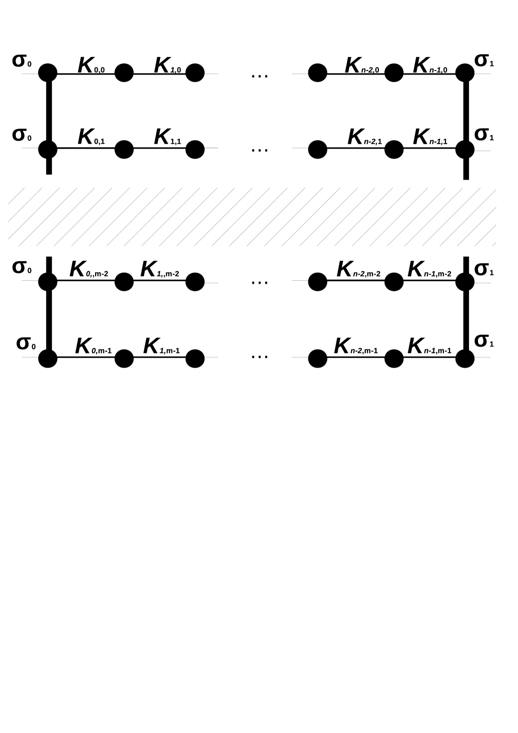
Figure 2: Construction of the first level bond from$mn$ zero level ones. here the utmost left $m$ spins, connected by vertical bold lines are $m$ copies of the spin$\sigma_{0},$the utmost right ones — of the spin $\sigma_{1}$.

Let $\sigma_{0}$ be the top spin, and $\sigma_{1}$ — the bottom one on the figure.e main procedure in the RSRG method is the one of partial summation in the partition function. Here it means the summation over all the spins, except $\sigma_{0}$ and $\sigma_{1}$. As a result, we get the contribution to the renormalized statistical weight of the model, which can be written as:

$$Z\left(\sigma_{0},\sigma_{1}\right)=\prod_{j=0}^{m-1}\left[\prod_{i=0}^{n-1}\hat{T}\left(K_{i,j}\right)\right]_{\sigma_{0}\sigma_{1}}=\prod_{j=0}^{m-1}\tilde{T}_{\sigma_{0}\sigma_{1}}^{\left(j\right)}\,,$$ (49)

One can easily ascertain, that the transfer matrix $\hat{\tilde{T}}$^(j) of the $j$-th chain may be expressed as:

$$\hat{\tilde{T}}^{\left(j\right)}=\prod_{i=0}^{n-1}\hat{T}\left(K_{i,j}\right)=\frac{1}{2\cosh\tilde{K}_{j}}\prod_{i=0}^{n-1}\left(2\cosh K_{i,j}\right)\hat{T}\left(\tilde{K}_{j}\right)\,,$$ (50)

where $\hat{T}$ is defined in Eq. (48), and the effective interaction of the $j$-th chain $\tilde{K}_{j}$ is:

$$\tanh\tilde{K}_{j}=\prod_{i=0}^{n-1}\tanh K_{ij}\,.$$ (51)

Then Eq. (49) may be rewritten as:

$$Z\left(\sigma_{0},\sigma_{1}\right)=z\left(\left\{K_{i,j}\right\}\right)\hat{T}_{\sigma_{0}\sigma_{1}}\left(K^{\left(1\right)}\right),\;$$ (52)

where

$$K^{\left(1\right)}=\sum_{j=0}^{m-1}\tilde{K}_{j}\,,$$ (53)

and

$$z\left(\left\{K_{i,j}\right\}\right)=\left[\prod_{j=0}^{m-1}\left(2\cosh\tilde{K}_{j}\right)\right]^{-1}\left[\prod_{j=0}^{m-1}\prod_{i=0}^{n-1}\left(2\cosh K_{i,j}\right)\right]$$ (54)

As a result, we have the RSRG equations for dimensionless interactions distribution,

$$\tilde{{\cal T}}_{q}=\overline{\prod_{i=0}^{n-1}\tanh^{q}K_{ij}}=\left[{\cal T}_{q}\right]^{n}\,,$$ (55)

$$\Phi_{1}\left(\xi\right)=\overline{\prod_{j=0}^{m-1}e^{i\xi\tilde{K}_{j}}}=\left[\tilde{\Phi}\left(\xi\right)\right]^{m}\,,$$ (56)

$$L_{1}\left(x\right)=\overline{\prod_{j=0}^{m-1}e^{x\tilde{K}_{j}}}=\left[\tilde{L}\left(x\right)\right]^{m}\,,$$ (57)

and the transformation formula for the free energy:

$$\bar{f}=T\left[\frac{1}{n}\overline{\ln\left(2\cosh\tilde{K}\right)}-\overline{\ln\left(2\cosh K\right)}\right]+\frac{1}{mn}\bar{f}_{1}\,.$$ (58)

References

- (1) S.F. Edwards and P.W. Anderson, J. Phys. F 5, 965 (1975)
- (2) M. Mezard, G. Parisi and M.A. Virasoro, Spin glass theory and beyond, World Scientific, Singapore, 1987
- (3) K. Binder and A.P. Young, Rev. Mod. Phys., 58, 801 (1986)
- (4) K.A. Fisher and J.A. Hertz, Spin Glasses, Cambridge University Press, 1993
- (5) V.S. Dotsenko, Phys. Usp. 36, 455 (1993)
- (6) H. Nishimori, Statistical Mechanics of Spin Glasses and Information Processing. An Introduction, Clarendon Press, Oxford, 2001
- (7) T. Castellani and A. Cavagna, J. Stat. Mech. P05012 (2005)
- (8) F. Zamponi, https://arxiv.org/abs/1008.4844
- (9) M. Advani, S. Lahiri and S. Ganguli, J. Stat. Mech., P03014 (2013); https://arxiv.org/abs/1301.7115
- (10) Frustrated Spin systems, H.T. Diep (ed.), World Scientific, Singapore, 2013
- (11) L.P. Kadanoff, Physics 2, 263 (1966)
- (12) A.A. Migdal, ZhETF 69, 810, 1457 (1975)
- (13) E. Efrati, Zhe Wang, A. Kolan and Leo P. Kadanoff, Rev. Mod. Phys., 86, 647 (2014); https://arxiv.org/abs/1301.6323v1
- (14) M. Droz and A. Malaspinas, Helv. Phys. Acta, 53, 214 (1980)
- (15) M.J. Thill and H.J. Hilhorst, J. Phys. I France 6, 67 (1996); https://arxiv.org/abs/cond-mat/9507092v1
- (16) E.Nogueira Jr, S. Coutinho, F.D. Nobre and E.M.F. Curado, Physica A, 271, 125 (1999); https://arxiv.org/abs/cond-mat/9906121v1
- (17) M.A. Moore, H. Bokil and B. Drossel, Phys. Rev. Lett. 81, 4252 (1998); https://arxiv.org/abs/cond-mat/9808140v1
- (18) E. Marinari, G. Parisi, J.J. Ruiz-Lorenzo and F. Zuliani, Phys. Rev. Lett., 82, 5176 (1999); https://arxiv.org/abs/cond-mat/9812324v1
- (19) O.R. Salmon and F. D. Nobre, Phys. Rev. E 79, 051122 (2009); https://arxiv.org/abs/0905.1088v1
- (20) M. Ohzeki, H. Nishimori and A.N. Berker, Phys. Rev. E 77, 061116 (2008); https://arxiv.org/abs/0802.2760v2
- (21) M. Castellana and G. Parisi, Phys. Rev. E 83, 041134 (2011); https://arxiv.org/abs/1006.5628v3
- (22) M. Castellana, Europhys. Lett., 95, 47014 (2011); https://arxiv.org/abs/1105.4955v2
- (23) Chuang Wang, Shao-Meng Qin and Hai-Jun Zhou, Phys. Rev. B, 90, 174201 (2014); https://arxiv.org/abs/1311.6577v2
- (24) C. Monthus, J. Stat. Mech., 2016, 043302 (2016); https://arxiv.org/abs/1601.05643v2
- (25) A.N. Samukhin, V.N. Prigodin, L. Jastrabík and A. Epstein, Phys. Rev. B 58, 11354 (1998); https://arxiv.org/abs/cond-mat/9808196
- (26) A.N. Vasil’ev, Functional methods in quantum field theory and statistics, Gordon & Breach, London, 1998