Solution of the ’sign problem’ in pair approximation

Abstract

The main difficulty for path integral Monte Carlo studies of Fermi systems results from the requirement of antisymmetrization of the density matrix and is known in literature as the ’sign problem’. To overcome this issue the new numerical version of the Wigner approach to quantum mechanics for treatment thermodynamic properties of degenerate systems of fermions has been developed. The new path integral representation of quantum Wigner function in the phase space has been obtained for canonical ensemble. Explicit analytical expression of the Wigner function accounting for Fermi statistical effects by effective pair pseudopotential has been proposed. Derived pseudopotential depends on coordinates, momenta and degeneracy parameter of fermions and takes into account Pauli blocking of fermions in phase space. The new quantum Monte-Carlo method for calculations of average values of arbitrary quantum operators has been proposed. To test the developed approach calculations of the momentum distribution functions and pair correlation functions of the degenerate ideal system of Fermi particles has been carried out in a good agreement with analytical distributions. Generalization of this approach for studies influence of interparticle interaction on momentum distribution functions of strongly coupled Fermi system is in progress.

1 Introduction

Over the last decades significant progress has been observed in theoretical studies of thermodynamic properties of strongly correlated fermions at non-zero temperatures, which is mainly conditioned by the application of numerical simulations (see review [1]). The reason for this success is the possibility of an explicit representation of the density matrix in the form of the Wiener path integrals [2] and making use of the Monte Carlo method for further calculations. The main difficulty for path integral Monte Carlo (PIMC) studies of Fermi systems results from the requirement of antisymmetrization of the density matrix [2]. As result all thermodynamic quantities are presented as the sum of alternating sign terms related to even and odd permutations and are equal to the small difference of two large numbers, which are the sums of positive and negative terms. The numerical calculation in this case is severely hampered. This difficulty is known in the literature as the ’sign problem’.

To overcome this issue some approaches have been developed [1, 3, 4, 5, 6, 7, 8, 9]. For example approaches [3, 5, 6] get ideal Fermi gas with very good accuracy. For interacting fermions the first results [5] have been obtained for the high densities for 33 particles and were now extrapolated to the thermodynamic limit very accurately in [6].

The ’fixed-node method’ [1, 7, 8, 9] is very widely known. However the main result of work [10] is that the ’fixed–node method’ can not reproduce even the well known ideal fermion density matrix and should be considered as an uncontrolled empirical approach for treatment thermodynamics of fermions. The analogous contradictions have been analytically obtained many years ago in [11] from virial decomposition of the many fermion ’fixed-node’ density matrix’.

In this work to treat the ’sign problem’ the new numerical version of the Wigner approach to quantum mechanics allowing studies of thermodynamic properties of the degenerate systems of fermions has been developed. The new path integral representation of quantum Wigner function in the phase space has been obtained for canonical ensemble. Explicit analytical expression of the Wigner function accounting for Fermi statistical effects by effective pair pseudopotential has been proposed. Derived pseudopotential depends on coordinates, momenta and degeneracy parameter of fermions and takes into account Pauli blocking of fermions in phase space. The new quantum Monte-Carlo method for calculations of average values of arbitrary quantum operators has been proposed. To test the developed approach calculations of the momentum distribution functions of the ideal system of Fermi particles has been carried out. Calculated by Monte Carlo method the momentum distributions and pair correlation functions for degenerate ideal fermions are in a good agreement with analytical distributions. Generalization of this approach for studies influence of interparticle interaction on momentum distribution functions of strongly coupled Fermi system is in progress. First results show appearance of long quantum ’tails’ in the Fermi distribution functions.

2 Wigner function for canonical ensemble

Average value of arbitrary quantum operator $\hat{A}$ can be written as its Weyl’s symbol $A(p,x)$, averaged over phase space with the Wigner function $W(p,x;\beta)$ [12, 13]:

$$\langle\hat{A}\rangle=\int\frac{dp\rmd x}{2\pi\hbar}A(p,x)W(p,x;\beta),$$ (1)

where the Weyl’s symbol of operator $\hat{A}$ is:

$$A(p,x)=\int\frac{d\xi}{2\pi\hbar}e^{-i\langle\xi|p\rangle/\hbar}\langle x-\xi/2|\hat{A}|x+\xi/2\rangle.$$ (2)

Weyl’s symbols for usual operators like $\hat{p}$, $\hat{x}$, $\hat{p}^{2}$, $\hat{x}^{2}$, $\hat{H}$, $\hat{H}^{2}$ etc. can be easily calculated directly from definition (2). The Wigner function of many particle system in canonical ensemble is defined as a Fourier transform of the off–diagonal matrix element of the density matrix operator in coordinate representation:

$$W(p,x;\beta)=Z(\beta)^{-1}\int{d\xi}e^{i\langle p|\xi\rangle/\hbar}\langle x-\xi/2|e^{-\beta\hat{H}}|x+\xi/2\rangle.$$ (3)

Here $\rho=\exp(-\beta\hat{H})$ is the density matrix operator of a quantum system of particles with the Hamiltonian $\hat{H}=\hat{K}+\hat{U}$ equal to the sum of kinetic $\hat{K}$ and potential energy $\hat{U}$ operators, while $\beta=1/k_{B}T$, $Z(\beta)$ is partition function.

There are well known difficulties in derivation of exact explicit analytical expression for Wigner function as operators of kinetic and potential energy in Hamiltonian do not commutate. To overcome this obstacle let us represent Wigner function in the form of path integral like in the well known case of the partition function. As example let us consider equilibrium a 3D two-component mass asymmetric electron–hole mixture consisting of $N_{e}$ electrons and $N_{h}$ holes ($N_{h}=N_{e}=N$) [14]. Here $Z(\beta)$ is defined as:

$$Z(N_{e},N_{h},V;\beta)=\frac{1}{N_{e}!N_{h}!\lambda_{e}^{3N_{e}}\lambda_{h}^{3N_{h}}}\sum_{\sigma}\int\limits_{V}dx\,\rho(x,\sigma;\beta),$$ (4)

where $\rho(x,\sigma;\beta)$ denotes the diagonal matrix elements of the density operator ${\hat{\rho}}=e^{-\beta{\hat{H}}}$. In equation (4), $x=\{x_{e},x_{h}\}$ and $\sigma=\{\sigma_{e},\sigma_{h}\}$ are the spatial coordinates and spin degrees of freedom of the electrons and holes, i.e. $x_{a}=\{x_{1,a}\ldots x_{l,a}\ldots x_{N_{a},a}\}$ and $\sigma_{a}=\{\sigma_{1,a}\ldots\sigma_{t,a}\ldots\sigma_{N_{a},a}\}$, $\lambda_{a}=\sqrt{\frac{2\pi\hbar\beta}{m_{a}}}$ is the thermal wave length, $l,t=1,\dots,N_{a}$ with $a=e,h$.

Of course, the density matrix elements of interacting quantum systems is not known (particularly for low temperatures and high densities), but it can be constructed using a path integral approach [2, 16] based on the operator identity $e^{-\beta{\hat{H}}}=e^{-\epsilon{\hat{H}}}\cdot e^{-\epsilon{\hat{H}}}\dots e^{-\epsilon{\hat{H}}}$, where $\epsilon=\beta/M$, which allows us to rewrite the integral in equation (4) as

$$\sum_{\sigma}\int\limits\rmd x^{(0)}\,\rho(x^{(0)},\sigma;\beta)=\int\limits\rmd x^{(0)}\dots\rmd x^{(m)}\dots dx^{(M-1)}\,\rho^{(1)}\cdot\rho^{(2)}\,\dots\rho^{(M-1)}\times$$

$$\sum_{\sigma}\sum_{P_{e}}\sum_{P_{h}}(\pm 1)^{\kappa_{P_{e}}+\kappa_{P_{h}}}\,{\cal S}(\sigma,{\hat{P}_{e}}{\hat{P}_{h}}\sigma^{\prime})\,{\hat{P}_{e}}{\hat{P}_{h}}\rho^{(M)}\big{|}_{x^{(M)}=x^{(0)},\sigma^{\prime}=\sigma}\,.$$ (5)

In equation (5) the index $m=0,\dots,M-1$ labels the off–diagonal high-temperature density matrices $\rho^{(m)}\equiv\rho\left(x^{(m)},x^{(m+1)};\epsilon\right)=\langle x^{(m)}|e^{-\epsilon{\hat{H}}}|x^{(m+1)}\rangle$.

With the error of order $1/M^{2}$ arising from neglecting commutator $\epsilon^{2}/2\left[K,U\right]$ in $e^{-\epsilon{\hat{H}}}\approx e^{-\epsilon{\hat{K}}}e^{-\epsilon{\hat{U}}}e^{-\epsilon^{2}/2\left[K,U\right]}\dots$ each high temperature factor can be presented in the form $\langle x^{(m)}|e^{-\epsilon{\hat{H}}}|x^{(m+1)}\rangle\approx\langle x^{(m)}|e^{-\epsilon{\hat{K}}}|x^{(m+1)}\rangle\langle x^{(m)}|e^{-\epsilon{\hat{U}}}|x^{(m)}\rangle$. In the limit $M\rightarrow\infty$ the error of the whole product of high temperature factors is equal to zero $(\propto 1/M)$ and this approach gives exact path integral representation of the partition function.

The spin gives rise to the spin part of the density matrix (${\cal S}$) with exchange effects accounted for by the permutation operators $\hat{P}_{e}$ and $\hat{P}_{h}$ acting on the electron and hole coordinates $x^{(M)}$ and spin projections $\sigma^{\prime}$. The sum is over all permutations with parity $\kappa_{P_{e}}$ and $\kappa_{P_{h}}$. So thermodynamic values are equal to very small difference between large (of order $N!/2$) positive and negative contributions giving by the even and odd permutations. The problem of accurate calculation of this difference is the well known sign problem for degenerate Fermi systems. The aim of this work is to develop simple and accurate approach for calculation this difference.

3 Exchange effects in pair approximation

To explain the basic ideas of our approach is enough to consider the simple system of ideal fermions (electrons and holes), so further $\hat{U}\equiv 0$. The hamiltonian of the system (${\hat{H}}={\hat{K}}={\hat{K}_{e}}+{\hat{K}_{h}}$) contains kinetic energy of electrons ${\hat{K}_{e}}$ and holes ${\hat{K}_{h}}$ respectively. Due to the commutativity of these operators the path integral representation of density matrix (5) is exact at any finite number $M$. For our purpose it is enough to consider the sum over permutations in pair approximation at $M=1$ (see [15]):

$$\sum_{\sigma}\sum_{P_{e}}\sum_{P_{h}}(\pm 1)^{\kappa_{P_{e}}+\kappa_{P_{h}}}\,{\cal S}(\sigma,{\hat{P}_{e}}{\hat{P}_{h}}\sigma_{a}^{\prime})\,{\hat{P}_{e}}{\hat{P}_{h}}\rho\,\big{|}_{x^{1}=x^{(0)},\sigma^{\prime}=\sigma}$$

$$=\sum_{\sigma_{e}}\sum_{P_{e}}(\pm 1)^{\kappa_{P_{e}}}{\cal S}(\sigma_{e},{\hat{P}_{e}}\sigma_{e}^{\prime})\,\rho_{e}\big{|}_{x_{e}^{1}=x_{e}^{(0)},\sigma_{e}^{\prime}=\sigma_{e}}\,$$

$$\times\sum_{\sigma_{h}}\sum_{P_{h}}(\pm 1)^{\kappa_{P_{h}}}{\cal S}(\sigma_{h},{\hat{P}_{h}}\sigma_{h}^{\prime})\,\rho_{h}\big{|}_{x_{h}^{1}=x_{h}^{(0)},\sigma_{h}^{\prime}=\sigma_{h}}$$

$$=\sum_{\sigma_{e}}\left\{1-\sum_{l<t}f^{2}_{e;lt}+\sum_{l,t,c}f_{e;lt}f_{e;lc}f_{e;tc}-\dots\right\}$$

$$\times\sum_{\sigma_{h}}\left\{1-\sum_{l<t}f^{2}_{h;lt}+\sum_{l,t,c}f_{h;lt}f_{h;lc}f_{h;tc}-\dots\right\}\approx\,$$

$$\approx\,\sum_{\sigma_{e}}\prod_{l<t}(1-f^{2}_{e;lt})\sum_{\sigma_{h}}\prod_{l<t}(1-f^{2}_{h;lt})=\sum_{\sigma}\exp(-\beta\sum_{l<t}\tilde{v}^{e}_{lt})\exp(-\beta\sum_{l<t}\tilde{v}^{h}_{lt})$$ (6)

where

$$f_{a;lt}=\exp(-\frac{\pi|x^{(0)}_{l,a}-x^{(0)}_{t,a}|^{2}}{\lambda_{a}^{2}})$$

$$\tilde{v}^{a}_{lt}=-kT\ln(1-f_{a;lt}f_{a;tl})=-kT\ln(1-\delta_{\sigma_{l,a}\sigma_{t,a}}\exp(-\frac{2\pi|x^{(0)}_{l,a}-x^{(0)}_{t,a}|^{2}}{\lambda_{a}^{2}}))$$ (7)

is exchange potential [15]. This formula shows that the first corrections accounting for the antisymmetrization of the density matrix result in the endowing particles by the pair exchange potential $\tilde{v}^{a}_{lt}$. Below to take into account exchange effects in Wigner functions we are going to use analogous pair potential depending on the phase space variables.

4 Path integral representation of Wigner function

Antisymmetrized Wigner function can be written in the form:

$$W(p,x;\beta)=\frac{1}{Z(\beta)N_{e}!N_{h}!\lambda_{e}^{3N_{e}}\lambda_{h}^{3N_{h}}}\sum_{\sigma}\sum_{P_{e}}\sum_{P_{h}}(\pm 1)^{\kappa_{P_{e}}+\kappa_{P_{h}}}{\cal S}(\sigma,{\hat{P}_{e}}{\hat{P}_{h}}\sigma^{\prime})\big{|}_{\sigma^{\prime}=\sigma}\,$$

$$\times\int d\xi e^{i\langle\xi|p\rangle}\langle x-\xi/2|\prod_{m=0}^{M-1}e^{-\epsilon{\hat{K}_{m}}}|{\hat{P}_{e}}{\hat{P}_{h}}(x+\xi/2)\rangle\,$$ (8)

Now replacing intermediate variables of integration $x^{(m)}$ in (8) (see (5)) for any permutation $P_{e}P_{h}$:

$$x_{e}^{(m)}=(P_{e}x_{e}-x_{e})\frac{m}{M}+x_{e}+q^{(m)}_{e}-\frac{(M-m)\xi_{e}}{2M}+\frac{mP_{e}\xi_{e}}{2M}\,$$

$$x_{h}^{(m)}=(P_{h}x_{h}-x_{h})\frac{m}{M}+x_{h}+q^{(m)}_{h}-\frac{(M-m)\xi_{h}}{2M}+\frac{mP_{h}\xi_{h}}{2M}\,$$ (9)

we obtain

$$W(p,x;\beta)=\frac{C(M)}{Z(\beta)N_{e}!N_{h}!\lambda_{e}^{3N_{e}}\lambda_{h}^{3N_{h}}}\sum_{\sigma}\sum_{P_{e}}\sum_{P_{h}}(\pm 1)^{\kappa_{P_{e}}+\kappa_{P_{h}}}{\cal S}(\sigma,{\hat{P}_{e}}{\hat{P}_{h}}\sigma^{\prime})\big{|}_{\sigma^{\prime}=\sigma}\,$$

$$\int d\xi\,\int dq^{(1)}\dots dq^{(M-1)}\exp\Biggl{\{}-\pi\frac{\langle\xi|P_{e}P_{h}+E|\xi\rangle}{2M}+i\langle\xi|p\rangle-\pi\frac{|P_{e}P_{h}x-x|^{2}}{M}$$

$$-\sum\limits_{m=0}^{M-1}\biggl{[}\pi|q^{(m)}-q^{(m+1)}|^{2}+\epsilon U\biggl{(}(P_{e}P_{h}x-x)\frac{m}{M}+x+q^{(m)}-\frac{(M-m)\xi}{2M}+\frac{mP_{e}P_{h}\xi}{2M}\biggr{)}\biggr{]}\Biggr{\}}$$

where angle brackets in $\langle p|\xi\rangle$ mean the scalar product of vectors $|p\rangle$ and $|\xi\rangle$, $E$ is unit matrix, while presenting permutation matrix $P_{e}P_{h}$ is equal to unit matrix with appropriately transposed columns. Here and further we imply that momentum and coordinate are dimensionless variables like $p_{l,a}\tilde{\lambda}_{a}/\hbar$ and $x_{l,a}/\tilde{\lambda}_{a}$, where $\tilde{\lambda}_{a}=\sqrt{\frac{2\pi\hbar\beta}{m_{a}M}}$. Here constant $C(M)$ as will be shown further is canceled in calculations of average values of operators. As a result, we have a new representation of Wigner function for canonical ensemble in the finite difference form of path integral. Let us note that integration here relates to the integration over the Wiener measure of all closed trajectories $\{q^{(0)},\dots,q^{(M-1)}\}$, which start and end at $q^{(0)}=q^{(M)}=x$. In fact, a particle is presented by the closed trajectory with characteristic size of order $\lambda_{a}=\sqrt{\frac{2\pi\hbar\beta}{m_{a}}}$ in coordinate space. This is manifestation of the uncertainty principle.

Then the Wigner function can be written in the following form:

$$W(p,x;\beta)=\frac{C(M)}{Z(\beta)N_{e}!N_{h}!\lambda_{e}^{3N_{e}}\lambda_{h}^{3N_{h}}}\sum_{\sigma}\sum_{P_{e}}\sum_{P_{h}}(\pm 1)^{\kappa_{P_{e}}+\kappa_{P_{h}}}{\cal S}(\sigma,{\hat{P}_{e}}{\hat{P}_{h}}\sigma^{\prime})\big{|}_{\sigma^{\prime}=\sigma}\,$$ (11)

$$\times\exp\Biggl{\{}-\pi\frac{|P_{e}P_{h}x-x|^{2}}{M}\Biggr{\}}\int dq^{(1)}\dots dq^{(M-1)}\exp\Biggl{\{}-\sum\limits_{m=0}^{M-1}\biggl{[}\pi|q^{(m)}-q^{(m+1)}|^{2}\biggr{]}\Biggr{\}}$$

$$\times\int d\xi\,\exp\Biggl{\{}-\pi\frac{\langle\xi|P_{e}P_{h}+E|\xi\rangle}{2M}+i\Biggl{\langle}\xi\Bigg{|}p\Biggr{\rangle}\Biggr{\}}.$$

In this paper we are going to allow for the exchange effects in the pair approximation by effective pseudopotental like have been discussed above (see (6)). So in this approximation Wigner function can be written as:

$$W(p,x;\beta)\approx\,\frac{C(M)}{Z(\beta)N_{e}!N_{h}!\lambda_{e}^{3N_{e}}\lambda_{h}^{3N_{h}}}\int dq^{(1)}\dots dq^{(M-1)}$$

$$\times\exp\Biggl{\{}-\sum\limits_{m=0}^{M-1}\biggl{[}\pi|q_{m}-q_{m+1}|^{2}\biggr{]}\Biggr{\}}\exp\Biggl{\{}-\frac{M}{4\pi}|p|^{2}\Biggr{\}}$$

$$\times\sum_{\sigma_{e}}\Biggl{\{}1-\sum_{l<t}\delta_{\sigma_{l,e}\sigma_{t,e}}\exp(-2\pi\frac{|x_{l,e}-x_{t,e}|^{2}}{M}\delta\biggl{(}\frac{(p_{l,e}-p_{t,e})\sqrt{M}}{2\pi}\biggr{)}\Biggr{\}}$$

$$\times\sum_{\sigma_{h}}\Biggl{\{}1-\sum_{l<t}\delta_{\sigma_{l,h}\sigma_{t,h}}\exp(-2\pi\frac{|x_{l,h}-x_{t,h}|^{2}}{M})\delta\biggl{(}\frac{(p_{l,h}-p_{t,h})\sqrt{M}}{2\pi}\biggr{)}\Biggr{\}}.$$ (12)

The main idea of deriving expression (4) can be explained on example of two electrons in 1D space. For two electrons the sum over permutations consist of two terms related to identical permutation (matrix $P$ is equal to unit matrix $E$) and non identical permutation (matrix $P$ is equal to matrix $E$ with transposed columns). To do integration in (11) over $\xi$ let us analyze eigenvalues of matrix $P+E$. For idetical permutation the eigenvalues are equal to each other and are equal to two, while the eigenvalues of matrix $P+E$ related to non identical permutation are equal to zero and two. Integration over $\xi$ for identical permutation is trivial, while for non identical permutation matrix $P+E$ before integration have to be presented in the form $P+E=ODO^{-1}$, where $D$ is diagonal matrix with zero and two as the diagonal elements. Here matrix $O$ and inverse matrix $O^{-1}$ are given by the formulas:

$$O=\left|\begin{array}[]{cc}1&1\\ -1&1\\ \end{array}\right|.$$

$$O^{-1}=\frac{1}{2}\left|\begin{array}[]{cc}1&-1\\ 1&1\\ \end{array}\right|.$$

Replacing variables by relation $|\zeta,\eta>=|O^{-1}|\xi>$ for each pair $(l,t)$ we can obtain expression (4).

To obtain the final expression we have to approximate delta-function in (4) by the standard Gaussian exponent with small parameter $\alpha$:

$$W(p,x;\beta)\approx\,\frac{C(M)}{Z(\beta)N_{e}!N_{h}!\lambda_{e}^{3N_{e}}\lambda_{h}^{3N_{h}}}\int dq^{(1)}\dots dq^{(M-1)}\exp\Biggl{\{}-\sum\limits_{m=0}^{M-1}\biggl{[}\pi|q^{(m)}-q^{(m+1)}|^{2}\biggr{]}\Biggr{\}}$$

$$\times\exp\Biggl{\{}-\frac{M}{4\pi}|p|^{2}\Biggr{\}}\sum_{\sigma}\exp(-\beta\sum_{l<t}v^{e}_{lt})\exp(-\beta\sum_{l<t}v^{h}_{lt})\Biggr{|}^{2}\Biggr{\}}$$ (13)

where

$$v^{a}_{lt}\approx-kT\ln\Biggl{\{}1-\delta_{\sigma_{l,a}\sigma_{t,a}}\exp\biggl{(}-2\pi\frac{|x_{l,a}-x_{t,a}|^{2}}{M}\biggr{)}\frac{\sqrt{M}}{2\pi\alpha}\exp\biggl{(}-\pi\frac{M|p_{l,a}-p_{t,a}|^{2}}{(2\pi\alpha)^{2}}\biggr{)}\Biggr{\}}$$

Note that the expression (4) contains explicitly term related the classical Maxwell distribution. The others terms account for the influence of exchange interaction on the momentum distribution function. In the limit of small $\alpha$ the rescaling $p$ by factor $\frac{\sqrt{M}}{2\pi\alpha}$ regularizes integration over momenta in (1) and allows to use simplified version of effective pair pseudopotential ($\pi$ is included in small $\alpha^{2}$):

$$v^{a}_{lt}\approx\,-kT\ln\Biggl{\{}1-\delta_{\sigma_{l,a}\sigma_{t,a}}\exp\biggl{(}-\frac{2\pi|x_{l,a}-x_{t,a}|^{2}}{\lambda^{2}_{a}}\biggr{)}\exp\biggl{(}-\frac{|(p_{l,a}-p_{t,a})\lambda_{a}|^{2}}{(2\pi\hbar)^{2}\alpha^{2}}\biggr{)}\Biggr{\}}$$

Momenta and coordinates are written here in natural units ($\lambda_{a}^{2}=\frac{2\pi\hbar^{2}\beta}{m_{a}}$).

5 Average values of quantum operators

For calculation of average values of quantum operators $\langle\hat{A}\rangle$ we are going to use the Monte Carlo method (MC) [17, 18]. To do this we have to use expression (4) presenting the discrete form of path integrals. As a result we obtain final expressions for MC calculations in the following form:

$$\langle\hat{A}\rangle=\frac{\left\langle A(p,x)\right\rangle_{w}}{\langle 1\rangle_{w}}.$$ (14)

Here brackets $\bigl{\langle}g(p,x,q_{1},\dots,q_{M-1})\bigr{\rangle}_{w}$ denote averaging of any function $g(p,x,q_{1},\dots,q_{M-1})$ with positive weight $w(p,x,q_{1},\dots,q_{M-1})$:

$$\langle g(p,x,q_{1},\dots,q_{M-1})\rangle_{w}$$

$$=\int{dp\rmd x}\int{dq_{1}\dots dq_{M-1}}g(p,x,q_{1},\dots,q_{M-1})w(p,x,q_{1},\dots,q_{M-1}).$$ (15)

while

$$w(p,x,q_{1},\dots,q_{M-1})=\exp\Biggl{\{}-\sum\limits_{m=0}^{M-1}\biggl{[}\pi|q^{(m)}-q^{(m+1)}|^{2}\biggr{]}\Biggr{\}}\exp\Biggl{\{}-\frac{M}{4\pi}\Bigg{|}p\Bigg{|}^{2}\biggr{)}\Biggr{\}},$$

$$\times\sum_{\sigma}\exp(-\beta\sum_{l<t}v^{e}_{lt})\exp(-\beta\sum_{l<t}v^{h}_{lt})$$ (16)

Note that denominator in (14) is equal to nominator with $A(p,x)=1$, so $C(M)$ in (4) is canceled.

Calculations of the average values of quantum operators depending only on coordinates of particles is more convenient and reasonable to carry out in configurational space by standard path integral Monte Karlo method (PIMC). Within considered above approach it can be done if we change the following functions:

$$\tilde{w}(x,q^{(1)},\dots,q^{(M-1)})=\exp\Biggl{\{}-\sum\limits_{m=0}^{M-1}\biggl{[}\pi|q^{(m)}-q^{(m+1)}|^{2}+\epsilon U(x+q^{(m)})\biggr{]}\Biggr{\}}$$

$$\times\sum_{\sigma}\exp(-\beta\sum_{l<t}\tilde{v}^{e}_{lt})\exp(-\beta\sum_{l<t}\tilde{v}^{h}_{lt}),$$

$$\tilde{h}(x,q^{(1)},\dots,q^{(M-1)})\equiv 1.$$ (17)

where $\tilde{v}^{a}_{lt}$ is defined by equation (7),

$$\langle g(x,q^{(1)},\dots,q^{(M-1)})\rangle_{\tilde{w}}=\int{dx}\int{dq^{(1)}\dots dq^{(M-1)}}g(x,q^{(1)},\dots,q^{(M-1)})\tilde{w}(x,q^{(1)},\dots,q^{(M-1)})$$ (18)

and

$$\langle{\tilde{\hat{A}}}\rangle=\frac{\left\langle\tilde{A}(x)\cdot\tilde{h}(x,q^{(1)},\dots,q^{(M-1)})\right\rangle_{\tilde{w}}}{\langle\tilde{h}(x,q^{(1)},\dots,q^{(M-1)})\rangle_{\tilde{w}}}.$$ (19)

6 Results of numerical calculations

We define momentum distribution functions and pair correlation functions for holes ($a=h$) and electrons ($a=e$) by the following expressions:

$$w_{a}(|p|)=\frac{\left\langle\delta(|p_{1,a}|-|p|)\cdot h(p,x,q^{(1)},\dots,q^{(M-1)})\right\rangle_{w}}{\langle h(p,x,q^{(1)},\dots,q^{(M-1)})\rangle_{w}}$$

$$g_{ab}(r)=\frac{\left\langle\delta(|x_{1,a}-x_{1,b}|-r)\cdot\tilde{h}(x,q^{(1)},\dots,q^{(M-1)})\right\rangle_{\tilde{w}}}{\langle\tilde{h}(x,q^{(1)},\dots,q^{(M-1)})\rangle_{\tilde{w}}}$$ (20)

where $\delta$ is delta function, $a$ and $b$ are types of the particles.

To test the developed approach we have carried out calculations of the path integral representation of Wigner function in the form (4). To extent the region of applicability of pair approximation we have used the small parameter $\alpha^{2}$ as adjustable function of the universal degeneracy parameter of ideal fermions $n\lambda^{3}$, namely $\alpha^{2}_{a}=0.00505+0.056n\lambda_{a}^{3}$ . Calculations have been done for two hundred particles each presented by twenty beads. Results have been obtained by averaging-out over one million particle configurations. To simplify calculations we fix the number of electrons and holes with the same spin projection equal to $N_{e}/2$ and $N_{h}/2$ respectively.

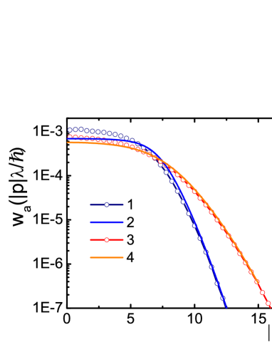
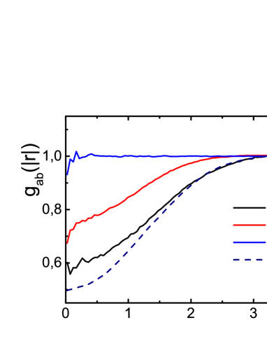
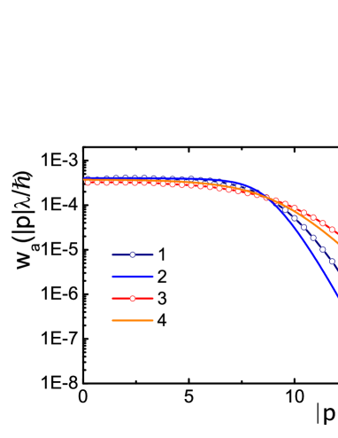
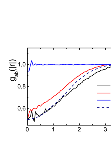
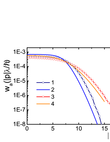
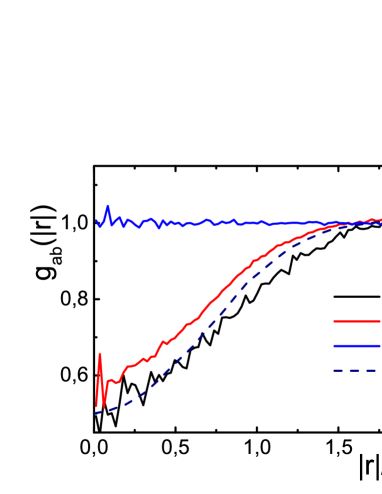
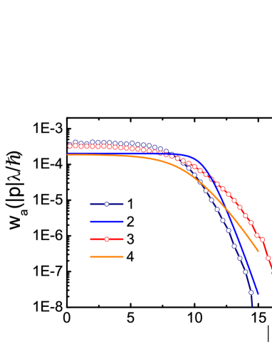
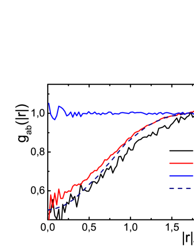
Figure 1: (Color online) The momentum distribution functions $w_{a}(|p|)$ (left panels) and pair correlation functions $g_{ab}(|r|),(a,b=e,h)$ (right panels) for ideal electron - hole plasma. Left panels: lines $1,3$ show PIMC distributions $w_{a}(|p|)$ scaled by ratio of Plank constant to the electron thermal wavelength ($\frac{\hbar}{\lambda_{e}}$), while lines $2,4$ demonstrate the ideal Fermi distributions for electrons and two times heavier holes respectively; Right panels: lines $1,2,3$ present PIMC electron – electron, hole – hole and electron – hole correlation functions scaled by Bohr radius respectively, while line 4 show results of analytical approximations [19] for electrons. Parameters of degeneracy $n\lambda^{3}_{e}$ for electrons are increasing from upper to bottom rows as $n\lambda^{3}_{e}=5,10,15,20$.

For ideal electron–hole plasma Figure 1 shows the momentum distributions $w_{a}(|p_{a}|),(a=e,h)$ and pair correlation functions $g_{ab}(|r|),(a,b=e,h)$ scaled by ratio of the Plank constant to the electron thermal wavelength ($\frac{\hbar}{\lambda_{e}}$) and Bohr radius ($a_{B}$) respectively. In left column of Figure 1 results of Monte Carlo calculations for electrons and holes are presented by lines 1 and 3, while lines 2 and 4 shows ideal Fermi distributions. Presented distribution functions are normalized to one. Let us note that holes is these calculations are two times heavier than electrons, so the related parameters of degeneracy is $2^{3/2}$ times smaller. As it follows from the analysis of Figure 1 agreement of PIMC calculations and analytical Fermi distribution are good enough up to parameter of degeneracy equal to $n\lambda_{e}^{3}=15$.

It necessary to stress that one of the reason of increasing discrepancy at large degeneracy of femions is limitation on available computing power allowing calculations with several hundred particles in Monte Carlo cell. When parameter of degeneracy is approaching $20$ the thermal electron wave length is of order Monte Carlo cell size and influence finite number of particles and periodic boundary conditions becomes significant as was tested by our calculations.

Right column of Figure 1 presents results of Monte Carlo calculations of pair correlation functions $g_{ab}(|r|),(a,b=e,h)$. Influence of Fermi repulsion at distance less than thermal wave length is evident enough. At the same time the electron—hole pair correlation functions are identically equal to one as exchange interaction between particle of different type is missing.

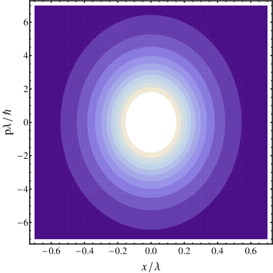
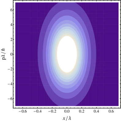
Figure 2: (Color online) Contour plots of the repulsive effective exchange pair pseudopotentials in phase space. Left panel: dark area $\beta v^{e}_{lt}\approx 0$, white area $\beta v^{e}_{lt}\geq 1.9$ , $m_{e}=1$. Right panel: dark area $\beta v^{h}_{lt}\approx 0$, white area $\beta v^{h}_{lt}\geq 1.5$ , $m_{h}=2$.

Presented results have been obtained in pair exchange approximation described by introduced above the effective pair pseudopotentials. Figure 2 presents contour plots of exchange pair pseudopotentials for parameter of degeneracy equal to $5.6$. Momenta and coordinates axises are scaled by the electron thermal wave length with Plank constant and factor ten for momentum. As before holes are two times heavier than electrons. As it follows from analysis of Figure 1 the Pauli blocking of fermions in phase space accounting for by these exchange pseudopotentials provides agreement of PIMC calculations and analytical Fermi distribution in wide ranges of fermion degeneracy and fermion momenta, where decay of the distribution functions is about of five orders of magnitude.

7 Conclusion

The new path integral representation of the quantum Wigner function in the phase space has been developed for canonical ensemble. Explicit analytical expression of the Wigner function accounting for Fermi statistical effects by effective pair pseudopotential has been obtained. Derived pseudopotential depends on coordinates, momenta and degeneracy parameter of fermions. The new quantum Monte-Carlo method for calculations of average values of arbitrary quantum operators has been proposed. To test the developed approach calculations of the momentum distribution function and pair correlation functions of the ideal system of Fermi particles has been carried out. Calculated by Monte Carlo method the momentum distributions for degenerate ideal fermions are in a good agreement with analytical Fermi distribution in a wide range of momentum and degeneracy parameter. Generalization of this approach for studies influence of interparticle interaction on momentum distribution functions of strongly coupled Fermi system is in progress. First results show appearance of long quantum ’tails’ in the Fermi distribution functions.

We acknowledge stimulating discussions with Profs. A.N. Starostin, Yu.V. Petrushevich, E.E. Son, I.L. Iosilevskii, M. Bonitz and V.I. Man’ko.

References

References

• [1] McMahon J M, Morales M A, Pierleoni C and Ceperley D 2012 Rev. Mod. Phys. 84 1607
• [2] Feynman R P and Hibbs A R 1965 Quantum Mechanics and Path Integrals (New York: McGraw-Hill)
• [3] Schoof T, Bonitz M, Filinov A, Hochstuhl D, and Dufty J W, 2011 Contrib. Plasma Phys. 51 687
• [4] Dornheim T, Groth S, Filinov A and Bonitz M 2015 New Journal of Physics 17 073017
• [5] Schoof T, Groth S, Vorberger J, and Bonitz M 2015 Phys. Rev. Lett. 115 130402
• [6] Dornheim T, Groth S, Sjostrom T, Malone F D, Foulkes W M C and Bonitz M 2016 Phys. Rev. Lett. 117 156403
• [7] Ceperley D 1991 J.Stat. Phys. 63 1237
• [8] Ceperley D 1992 Phys. Rev. Let. 69 331
• [9] Militzer B and Pollock R 2000 Phys. Rev. E 61, 3470
• [10] Filinov V S 2014 High Temperature, 52, 615
• [11] Filinov V 2001 J. Phys. A: Math. Gen. 34, 1665
• [12] Wigner E P 1932 Phys. Rev. 40 749
• [13] Tatarskii V 1983 Sov. Phys. Uspekhi 26 311
• [14] Filinov V S et al. 2007 Physical review E 75 036401
• [15] Huang K 1966 Statistical mechanics (Moscow, Mir)
• [16] Zamalin V M, Norman G E and Filinov V S, 1977 The Monte – Carlo Method in Statistical Thermodynamics, Nauka, Moscow.
• [17] Metropolis N et al. 1953 Journal of Chemical Physics, 21 1087
• [18] Hasting W K 1970 Biometrika 57 97
• [19] Bosse J., Pathak K. N., Singh G. S. 2011 Phys. Rev. E 84 042101