Computing geometric Lorenz attractors with arbitrary precision

Abstract

The Lorenz attractor was introduced in 1963 by E. N. Lorenz as one of the first examples of strange attractors. However Lorenz’ research was mainly based on (non-rigourous) numerical simulations and, until recently, the proof of the existence of the Lorenz attractor remained elusive. To address that problem some authors introduced geometric Lorenz models and proved that geometric Lorenz models have a strange attractor. In 2002 it was shown that the original Lorenz model behaves like a geometric Lorenz model and thus has a strange attractor.

In this paper we show that geometric Lorenz attractors are computable, as well as their physical measures.

1 Introduction

The system of equations

$$\left\{\begin{array}[c]{c}x^{\prime}=\sigma(y-x)\\ y^{\prime}=\rho x-y-xz\\ z^{\prime}=xy-\beta z\end{array}\right.$$ (1.1)

is called the Lorenz system, where $\sigma,\beta,$ and $\rho$ are parameters. This system was first studied by E. N. Lorenz in 1963 [13] as a simplified model of atmosphere convection in an attempt to understand the unpredictable behavior of the weather. Lorenz’s original numerical simulations, where the parameters were given by $\sigma=10$, $\beta=8/3$, and $\rho=28$, suggested that for any typical initial condition, the system would eventually tend to a same limit set with a rather complicated structure – the Lorenz (strange) attractor. Moreover, the dynamics on this attractor seemed to magnify small errors very rapidly, rendering impractical to numerically simulate an individual trajectory for an extended period of time.

The Lorenz system became a landmark in the modern paradigm of the numerical study of chaos: instead of studying trajectories individually, one should study the limit set of a typical orbit, both as a spatial object and as a statistical distribution [15]. However, proving the existence of the Lorenz attractor in a rigorous fashion turned out to be no easy task; indeed, the problem was listed in 1998 by Smale as one of the eighteen unsolved problems he suggested for the 21st century [17].

In 1979, based on the behavior observed in the numerical simulations of (1.1), Afraimovich, Bykov, and Shil’nikov [1], and Guckenheimer and Williams [11] originated the study of flows satisfying a certain list of geometric properties intended to capture the observed numerically simulated behavior. In particular, they proved that any such flow must contain a strange attractor, which supports a unique invariant probability distribution that describes the limiting statistical behavior of almost any initial condition. These examples came to be known as geometric Lorenz models, and the strange attractor contained in a geometric Lorenz flow is called the geometric Lorenz attractor.

Using a combination of normal form theory and rigorous numerics, Tucker [18] provided, in 2002, a formal proof on the existence of the Lorenz attractor by showing that the geometric Lorenz models do indeed correspond to the Lorenz system (1.1) for certain parameters. Since a geometric Lorenz model supports a strange attractor, so does the Lorenz system (1.1).

In this note, we examine computability of geometric Lorenz attractors and their physical measures. By definition, a computable set in the plane can be visualized on a computer screen with an arbitrarily high magnification, and integrals with respect to a computable probability measure can be generated by a computer with arbitrary precision. Our main result is the following:

Main Theorem. For any geometric Lorenz flow, if the data defining the flow are computable, then its attractor is a computable subset of $\mathbb{R}^{3}$. Moreover, the physical measure supported on this attractor is a computable probability measure.

We note that, although computer generated images of the “butterfly shaped” Lorenz attractor abound in the internet, these images are not rigorous computations. In particular, their existence does not necessarily mean that the attractor is actually computable. In fact, an equally famous collection of invariant sets, namely Julia sets, whose computer images are also abundant, was shown to contain non computable members [5].

In order to make our results accessible to a wide audience, we have made an effort to work directly from the definitions, making the proofs as self-contained as possible.

2 Preliminaries

2.1 Computable analysis

Roughly speaking, an object is computable if it can be approximated by computer-generated approximations with an arbitrarily high precision. Formalizing this idea to carry out computations on infinite objects such as real numbers, we encode those objects as infinite sequences of rational numbers (or equivalently, sequences of any finite or countable set $\Sigma$ of symbols), using representations (see [20] for a complete development). A represented space is a pair $(X;\delta)$ where $X$ is a set, $\mbox{dom}(\delta)\subseteq\Sigma^{\mathbb{N}}$, and $\delta:\subseteq\Sigma^{\mathbb{N}}\to X$ is an onto map (“$\subseteq\Sigma^{\mathbb{N}}$” is used to indicate that the domain of $\delta$ may be a subset of $\Sigma^{\mathbb{N}}$). Every $q\in\mbox{dom}(\delta)$ such that $\delta(q)=x$ is called a $\delta$-name of $x$ (or a name of $x$ when $\delta$ is clear from context). Naturally, an element $x\in X$ is computable if it has a computable name in $\Sigma^{\mathbb{N}}$ (the notion of computability on $\Sigma^{\mathbb{N}}$ is well established). In this note, we use the following particular representations for points in $\mathbb{R}^{n}$; for closed subsets of $\mathbb{R}^{n}$; and for continuous functions defined on $I_{1}\times I_{2}\times\cdots\times I_{n}\subset\mathbb{R}^{n}$, where $I_{j}$’s are intervals:

• For a point $x\in\mathbb{R}^{n}$, a name of $x$ is a sequence $\{r_{k}\}$ of points with rational coordinates satisfying $|x-r_{k}|<2^{-k}$. Thus $x$ is computable if there is a Turing machine (or a computer program or an algorithm) that outputs a rational $n$-tuple $r_{k}$ on input $k$ such that $|r_{k}-x|<2^{-k}$; for a sequence $\{x_{j}\}$, $x_{j}\in\mathbb{R}^{n}$, a name of $\{x_{j}\}$ is a double sequence $\{r_{j,k}\}$ of points with rational coordinates satisfying $|x_{j}-r_{j,k}|<2^{-k}$.

• For a closed subset $A$ of $\mathbb{R}^{n}$, a name of $A$ consists of a pair of an inner-name and an outer-name; an inner-name is a sequence dense in $A$ and an outer-name is a sequence of balls $B(a_{n},r_{n})=\{x\in\mathbb{R}^{n}\,:\,d(a_{n},x)<r_{n}\}$, $a_{n}\in\mathbb{Q}^{n}$ and $r_{n}\in\mathbb{Q}$, exhausting the complement of $A$, i.e., $\mathbb{R}^{n}\setminus A=\bigcup_{n=1}^{\infty}B(a_{n},r_{n})$. $A$ is said to be r.e. closed if the sequence (dense in $A$) is computable; co-r.e. closed if the sequences $\{a_{n}\}$ an $\{r_{n}\}$ are computable; and computable if it is r.e. and co-r.e.. For a compact set $K$, a name of $K$ consists of a name of $K$ as a closed set and a rational number $r$ such that $K\subseteq B(0,r)$. By the definition, a planar computable closed set can be visualized on a computer screen with an arbitrarily high magnification.

• For every continuous function $f$ defined on $I_{1}\times I_{2}\times\cdots\times I_{n}\subseteq\mathbb{R}^{n}$, where $I_{j}$ is an interval with endpoints $a_{j}$ and $b_{j}$, a name of $f$ is a double sequence $\{P_{k,l}\}$ of polynomials with rational coefficients satisfying $d_{k}(P_{k,l},f)<2^{-l}$, where $d_{k}(g,f)=\max\{|g(x)-f(x)|\,:\,a_{j}+2^{-k}\leq x_{j}\leq b_{j}-2^{-k},1\leq j\leq n\}$ ($d_{k}(g,f)=0$ if $[a_{j}+2^{-k},b_{j}-2^{-k}]=\emptyset$). Thus, $f$ is computable if there is an (oracle) Turing machine that outputs $P_{k,l}$ (more precisely coefficients of $P_{k,l}$) on input $k,l$ satisfying $d_{k}(P_{k,l},f)<2^{-l}$.

• For every $C^{m}$ function $f$ defined on $E=I_{1}\times I_{2}\times\cdots\times I_{n}\subseteq\mathbb{R}^{n}$, where $I_{j}$ is an interval with endpoints $a_{j}$ and $b_{j}$, a ($C^{m}$) name of $f$ is a double sequence $\{P_{k,l}\}$ of polynomials with rational coefficients satisfying

  $$d^{m}_{k}(P_{k,l},f)<2^{-l},$$

  where

  $$d^{m}_{k}(g,f)=\max_{0\leq i\leq m}\max\{|D^{i}g(x)-D^{i}f(x)|\,:\,a_{j}+2^{-k}\leq x_{j}\leq b_{j}-2^{-k}\}$$

  ($d^{m}_{k}(g,f)=0$ if $[a_{j}+2^{-k},b_{j}-2^{-k}]=\emptyset$). We observe that a $C^{m}$ name of $f$ contains information on both $f$ and $Df,D^{2}f,\ldots,D^{m}f$, in the sense that $(P_{1},P_{2},\ldots)$ is a $\rho$-name of $f$ while $(D^{i}P_{1},D^{i}P_{2},\ldots)$ is a $\rho$-name of $D^{i}f$. See [22] for further details.

The notion of computable maps between represented spaces now arises naturally. A map $\Phi:(X;\delta_{X})\to(Y;\delta_{Y})$ between two represented spaces is computable if there is a computable map $\phi:\subseteq\Sigma^{\mathbb{N}}\to\Sigma^{\mathbb{N}}$ such that $\Phi\circ\delta_{X}=\delta_{Y}\circ\phi$. Informally speaking, this means that there is a computer program that outputs a name of $\Phi(x)$ when given a name of $x$ as input [4].

2.2 Geometric Lorenz models

We briefly describe a geometric Lorenz model taken from [10] (see section 5.7 [10] for more details).

For the parameter values $\sigma=10$, $\beta=8/3$, and $\rho=28$, the Lorenz system (1.1) has three equilibrium points: the origin, $q_{-}$, and $q_{+}$; both $q_{-}$ and $q_{+}$ lie on the plane $z=\rho-1=27$. The numerical simulations of (1.1) for these parameter values show that the Lorenz flow rotates around the equilibria $q_{\pm}$ and intersects the plane $z=27$ infinitely many times, thus indicating that there is a return map with the cross section $z=27$. Geometric Lorenz models are constructed based upon the behavior of this numerically observed return map.

It is proved (cf. [10], [12] and references therein) that a flow satisfying the following properties exists (see Figure 1): The flow has three equilibrium points: the origin of $\mathbb{R}^{3}$ and $Q_{\pm}$; for the origin, its stable manifold is the $yz$-plane while its unstable manifold intersects the plane $z=27$ from above at two points, say $\rho^{+}=(r^{-},t^{-})$ and $\rho^{-}=(r^{+},t^{+})$; for $Q_{-}$ and $Q_{+}$, they lie in the plane $z=27$ and have integer coordinates $(-m,-n,27)$ and $(m,n,27)$, their stable lines are parallel to the $y$-axis, and the other two eigenvalues at $Q_{\pm}$ are assumed to be complex with positive real part, as is the Lorenz system. Let $\Sigma$ be a rectangle contained in the plane $z=27$ such that $\rho^{\pm}$ is contained in $\Sigma$, the two opposite sides of $\Sigma$ parallel to the $y$-axis pass through the equilibrium points $Q_{-}$ and $Q_{+}$, and these two sides form portions of the stable lines at $Q_{-}$ and $Q_{+}$. Let $D$ be the intersection of the $yz$-plane and $\Sigma$. The flow has the following features: $\Sigma$ is a cross section for the flow; all trajectories go downwards through $\Sigma$; all trajectories originating in $\Sigma$ and not entering $D$ spiral around $Q_{-}$ or $Q_{+}$ and return to $\Sigma$ as time moves forward; all trajectories beginning at points in $D$ tend to the origin as time moves forward and never return to $\Sigma$; and there is a Poincaré return map $F:\Sigma_{-}\bigcup\Sigma_{+}\to\Sigma$, where $\Sigma_{-}=\{(x,y)\in\Sigma|x<0\}$ and $\Sigma_{+}=\{(x,y)\in\Sigma|x>0\}$.

Let $V=\{(x,y)|r^{-}\leq x\leq r^{+},\,-27\leq y\leq 27\}$ (the number 27 is arbitrarily chosen; other positive numbers can be used as well). The Lorenz flow has also the property that all points in the interior of $\Sigma\setminus D$ have a trajectory which will eventually reach $V$ and $F(V\setminus D)\subseteq V$ (see Figure 4). Thus we can restrict the analysis of the flow to $V$. The Poincaré return map $F$ has the following properties on $V$:

• The set $\mathcal{F}$, $\mathcal{F}=\{\mbox{$x$=constant}\}$, is invariant under the action of $F$. In other words, the $x$-coordinate of the image $F(x_{0},y_{0})$ depends only on $x_{0}$.

• There are functions $f$ and $g$ such that $F$ can be written as

  $$F(x,y)=(f(x),g(x,y))\text{ \ \ for }x\neq 0$$

  and $F(-x,-y)=-F(x,y)$.

• $f^{\prime}(x)>\sqrt{2}$ for $x\neq 0$ and $f^{\prime}(x)\rightarrow\infty$ as $x\rightarrow 0$; $0<f(r^{+})<r^{+}$ and $r^{-}<f(r^{-})<0$ (recall that the unstable manifold of the origin first intersects $V$ from above at points $\rho^{+}$ and $\rho^{-}$).

• $0<\partial g/\partial y\leq c<1/\sqrt{2}$ and $0<\partial g/\partial x\leq c$ for $x\neq 0$ and $\partial g/\partial y\rightarrow 0$ as $x\rightarrow 0$ (see [12, Section 14.4]). Without loss of generality, $c$ can be assumed to be a rational number and $\partial g/\partial y\rightarrow 0$ to be monotonic as $x\to 0$.
  

A consequence of (F-2)-(F-4) is that (see [12, Section 14.4]):

• $\lim_{x\rightarrow 0^{-}}F(x,y)=(r^{+},t^{+})$ and $\lim_{x\rightarrow 0^{+}}F(x,y)=(r^{-},t^{-})$, where $\rho^{-}=(r^{+},t^{+})$ and $\rho^{+}=(r^{-},t^{-})$. The symmetry property (F-2) implies that $r^{-}<0<r^{+}$ and $r^{-}=-r^{+}$.
  

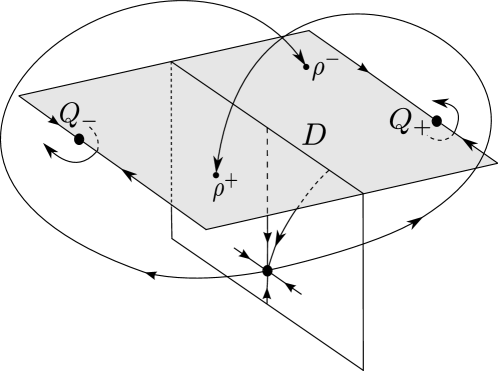
Figure 1: The geometric model for the Lorenz system.

The image of $\Sigma$ by $F$ is depicted in Figure 2.

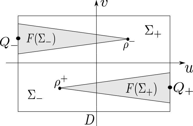
Figure 2: The Poincaré map $F$ on the cross-section $\Sigma$.

Figure 3 shows a picture of the flow, where $\Sigma$ is the upper surface of the solid and the flow is tangent to the curved surfaces of the solid and to the bottom segment. On the front and back surfaces, the flow is into the solid while the trajectories emerge from the vertical ends. These emergent trajectories are continued around so that $F$ describes the return map for $V$. This flow, denoted by $\phi_{t}$, $t\in\mathbb{R}$ and acting on $M=\{\phi_{t}(x,y,z):(x,y,z)\in V\times\{27\},t\in\mathbb{R}^{+}\}$ is called a geometric Lorenz flow.

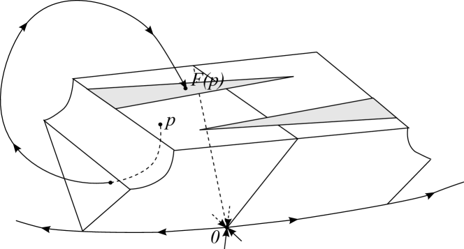
Figure 3: A three-dimensional representation of the geometric Lorenz flow.

It is shown in [10] that

$$A={\displaystyle\bigcap\limits_{n\geq 0}}\overline{F^{n}(V\setminus D)}$$

is the intersection of the attractor for the geometric Lorenz flow with $V$ and that

$$\mathcal{A}=\left({\displaystyle\bigcup\limits_{t\in\mathbb{R}}}\phi_{t}(A)\right)\cup\{(0,0,0)\}$$

is an attractor for the geometric Lorenz flow $\phi_{t}$; this attractor is a Lorenz-like strange attractor. Note that $F$ is defined on $V\setminus D$. Thus $F^{2}(V\setminus D)$ is understood as of $F(F(V\setminus D)\setminus D)$ and, inductively, $F^{n+1}(V\setminus D)=F(F^{n}(V\setminus D)\setminus D)$.

We mention in passing that the geometric Lorenz model is not unique; in fact, any flow which satisfies the geometric conditions listed above contains a Lorenz-like strange attractor, thus it is a geometric Lorenz flow. As usual, one might also need to use some reparametrization of the model to ensure that it behaves like described in this section (it has a fixed point on the origin, etc.). All computability results stated in this paper are relative to that (eventual) reparametrization.

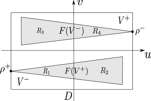
Figure 4: The Poincaré map on the cross-section $V$.

3 Computability of geometric Lorenz attractors

In this section, we show that the strange attractor $\mathcal{A}$ contained in a geometric Lorenz flow is uniformly computable from the data defining the flow. Thus, if the data defining the flow is computable, then so is $\mathcal{A}$; by definition this means that $\mathcal{A}$ can be visualized on a computer screen with an arbitrary high magnification.

We begin by studying computability of the set $A$, for $\mathcal{A}$ consists of the trajectories passing through $A$. We start by showing that $A$ is uniformly computable from $F$ and $\rho^{\pm}$.

Theorem 1

The operation $(F,\rho^{\pm})\to A$ is computable.

Proof. We show that $A$ is computable by making use of the “constructive” definition of $A$, $A=\bigcap_{n\geq 0}\overline{F^{n}(V\setminus D)}$. Let $A_{n}=\overline{F^{n}(V\setminus D)}$. In Propositions 4 and 5 below, we show that

1. the sequence $\{A_{n}\}$ is computable from $F$ and $\rho^{\pm}$ and

2. $\max_{(x,y)\in V}|d_{A_{n+1}}(x,y)-d_{A_{n}}(x,y)|\leq 108c^{n}$ (see (F-4) for definition of the number $c$).

Then it follows from (d) and (e) of Lemma 3 that $A$ is computable from $F$ and $\rho^{\pm}$ since $A_{n+1}\subseteq A_{n}$. Propositions 4 and 5, together with their proofs, are presented below.   

We will need the following lemmas, which will be also needed in several later proofs. Recall that an operation $\mathcal{O}:X\to Y$ is computable if there is a Turing algorithm that, for any given name of $x$ as input, outputs a name of $\mathcal{O}(x)$.

Lemma 2

The operation $(f,b,\beta)\to f_{1}$ is computable, where $f:(0,b]\to\mathbb{R}$ is a continuous function with the following properties: (i) it is monotonic on $(0,b]$ and (ii) $f(x)\to\beta$ as $x\to 0^{+}$, and

$$f_{1}(x)=\left\{\begin{array}[c]{ll}f(x)&x\in(0,b]\\ \beta&x=0\end{array}\right.$$

Similarly, the operation $(f,a,\beta)\to f_{2}$ is computable, where $f:[a,0)\to\mathbb{R}$ is a continuous function, with the following properties: (i) it is monotonic on $[a,0)$ and (ii) $f(x)\to\beta$ as $x\to 0^{-}$, and

$$f_{2}(x)=\left\{\begin{array}[c]{ll}f(x)&x\in[a,0)\\ \beta&x=0\end{array}\right.$$

Proof. The proof is straightforward, thus omitted.   

Lemma 3

The following results can be found in Chapters 5 & 6 [20]. Assume that $A$, $B$, and $K$ are subsets of $\mathbb{R}^{n}$.

• The operation $(f,K)\to f[K]$ for continuous $f$ and compact $K$ is computable.

• The union $(A,B)\to A\bigcup B$ of compact sets is computable.

• The operation $(f,a,b)\to(f^{-1},c,d)$ for continuous strictly monotonic $f$ is computable, where $f^{-1}$ is the inverse of $f$ and $f[a,b]=[c,d]$.

• The operation $((f_{i})_{i\in\mathbb{N}},K)\to f$, $f(x)=\lim_{i\to\infty}f_{i}(x)$, is computable, where $\max_{x\in K}|f_{i}(x)-f_{j}(x)|\leq C\cdot c^{i}$ for all $j>i$, $K$ is compact, $C$ is a rational number, and $0<c<1$.

• The operations $K\to d_{K}$ and $d_{K}\to K$ for non-empty compact sets $K$ are computable, where $d_{K}$ is the distance function defined on $K$: $d_{K}(x)=dist(x,K)$.

Proposition 4

$\{A_{n}\}$ is computable.

Proof. Let us first give an idea on how to compute the sequence $\{A_{n}\}$ from $F$ and $\rho^{\pm}$. Intuitively one may attempt to compute $F^{n}(V\setminus D)$ directly and then compute its closure. However, since $F^{n}(V\setminus D)$ is neither open nor closed, it cannot be computed from $F^{n}$, although $F^{n}$ is computable from $F$ for every $n\in\mathbb{N}$. A possible solution is to extend $F$ to be defined on $V$ and then compute $F^{n}(V)$. But this method also fails to work here – $F$ is singular along $D\subseteq V$ and therefore it cannot be extended to a continuous function on $V$. Nevertheless, we observe that if we break $F$ into two half functions, each of them defined on one half of $V\setminus D$, then we can extend each half function continuously to be also defined on $D$ (from property (F-5)); moreover, the extension is computable from the given data. And so if we can show that the iterations of the two half functions yield $\overline{F^{n}(V\setminus D)}$ and are computable from $F$ and $\rho^{\pm}$, we have the desired sets $A_{n}$.

Now for the details. Recall that $V=\{(x,y)|r^{-}\leq x\leq r^{+},\,-27\leq y\leq 27\}$. Let $V^{+}=\{(x,y)\in V\,|\,x\geq 0\}$ and $V^{-}=\{(x,y)\in V\,|\,x\leq 0\}$; let $I^{+}=\{x\,|\,0\leq x\leq r^{+}\}$, $I^{-}=\{x\,\,|r^{-}\leq x\leq 0\}$, and $I=[r^{-},r^{+}]$. It is then clear that $V$, $V^{+}$, $V^{-}$, $I$, $I^{+}$, and $I^{-}$ are all computable from $r^{\pm}$. Also recall that $F(x,y)=(f(x),g(x,y))$ on $V\setminus D$, $D=\{(0,y)\,|\,-27\leq y\leq 27\}$. Define

$$f^{+}:I^{+}\rightarrow I,\quad f^{+}(x) =\left\{\begin{array}[c]{ll}f(x)&0<x\leq r^{+}\\ r^{-}&x=0\end{array}\right.$$

$$f^{-}:I^{-}\rightarrow I,\quad f^{-}(x) =\left\{\begin{array}[c]{ll}f(x)&r^{-}\leq x<0\\ r^{+}&x=0\end{array}\right.$$

$$g^{+}:V^{+}\rightarrow[-27,27],\quad g^{+}(x,y) =\left\{\begin{array}[c]{ll}g(x,y)&0<x\leq r^{+}\\ t^{-}&x=0\end{array}\right.$$

$$g^{-}:V^{-}\rightarrow[-27,27],\quad g^{-}(x,y) =\left\{\begin{array}[c]{ll}g(x,y)&r^{-}\leq x<0\\ t^{+}&x=0\end{array}\right.$$

By (F-3) and (F-5) (that is, $f^{\prime}(x)>\sqrt{2}$ for $x\neq 0$, $\lim_{x\to 0^{-}}F(x,y)=(r^{+},t^{+})$ and $\lim_{x\to 0^{+}}F(x,y)=(r^{-},t^{-})$), it follows that $f(x)\nearrow r^{+}$ when $x\to 0^{-}$ and that $f(x)\searrow r^{-}$ as $x\to 0^{+}$. Then it follows from Lemma 2 that both $f^{+}$ and $f^{-}$ are computable. A similar argument shows that $g^{+},g^{-}$ are computable.

Let $F^{\pm}(x,y)=(f^{\pm}(x),g^{\pm}(x,y))$, $(x,y)\in V^{\pm}$, where $f^{\pm}$ ($g^{\pm}$) is either $f^{+}$ or $f^{-}$ ($g^{+}$ or $g^{-}$). Then $F^{\pm}$ is computable from $f^{\pm}$ and $g^{\pm}$; thus it is computable.

Now, recall that $A_{n}=\overline{F^{n}(V\setminus D)}$ by definition. It can be shown that

$$A_{n}=\overline{F(A_{n-1}\setminus D)},\quad n\geq 1$$ (3.1)

by induction as follows: Let $A_{0}=V$. Then $A_{1}=\overline{F(V\setminus D)}=\overline{F(A_{0}\setminus D)}$. Assume that $A_{n}=\overline{F(A_{n-1}\setminus D)}$. We show that $A_{n+1}=\overline{F(A_{n}\setminus D)}$. By definition,

$$A_{n+1} = \overline{F^{n+1}(V\setminus D)}$$

$$= \overline{F(F^{n}(V\setminus D)\setminus D)}$$

$$\subseteq \overline{F\left(\overline{F^{n}(V\setminus D)}\setminus D\right)}$$

$$= \overline{F(A_{n}\setminus D)}.$$

It remains to show that $\overline{F(A_{n}\setminus D)}\subseteq A_{n+1}$. Since $A_{n+1}$ is closed (in $\mathbb{R}^{2}$), it suffices to show that $F(A_{n}\setminus D)\subseteq A_{n+1}$. Since $F(A_{n}\setminus D)=F(A_{n}\cap(V\setminus D))$, $A_{n}\cap(V\setminus D)$ is closed in $V\setminus D$, and $F$ is continuous on $V\setminus D$, it then follows that

$$F(A_{n}\setminus D) = F(A_{n}\cap(V\setminus D))$$

$$= F\left(\overline{F^{n}(V\setminus D)}\cap(V\setminus D)\right)$$

$$\subseteq \overline{F(F^{n}(V\setminus D)\cap(V\setminus D))}$$

$$= A_{n+1}.$$

Therefore $A_{n+1}=\overline{F(A_{n}\setminus D)}$.

We also note that, following (F3), $f:I\setminus\{0\}\to I\setminus\{r^{+},r^{-}\}$ is a surjective map. Combining this fact with (F4) and (F5) we conclude that

$$\rho^{-},\,\rho^{+}\in A_{n},\quad n\geq 0.$$ (3.2)

It now follows from (3.1) and (3.2) that

$$A_{n}=\overline{F(A_{n-1}\setminus D)}=F^{+}(A_{n-1}\cap V^{+})\bigcup F^{-}(A_{n-1}\cap V^{-}).$$ (3.3)

Let $\mathcal{C}=\{K\subseteq V\,|\,\mbox{$K$ is closed in $V$}\}$ and let $\alpha$ be a map from $\mathcal{C}$ to $\mathcal{C}$ defined by the following formula: for each $K\in\mathcal{C}$,

$$\alpha(K)=F^{+}(K\cap V^{+})\bigcup F^{-}(K\cap V^{-})\bigcup\{\rho^{-},\rho^{+}\}.$$ (3.4)

Note that $F(K\cap(V\setminus D))=F^{+}(K\cap(V^{+}\setminus D))\bigcup F^{-}(K\cap(V^{-}\setminus D))$. Then it follows from (F5) that $\overline{F(K\cap(V\setminus D))}\bigcup\{\rho^{-},\rho^{+}\}=F^{+}(K\cap V^{+})\bigcup F^{-}(K\cap V^{-})\bigcup\{\rho^{-},\rho^{+}\}$; i.e.,

$$\alpha(K)=\overline{F(K\cap(V\setminus D))}\bigcup\{\rho^{-},\rho^{+}\}.$$ (3.5)

In order to prove that $\{A_{n}\}$ is computable, it suffices to show that the map $\alpha$ is computable since $A_{n}=\alpha^{n}(V)$. Towards this end, it suffices to show that, for each $K\in\mathcal{C}$, (i) $\alpha$ maps every outer-name of $K$ to an outer-name of $\alpha(K)$ and (ii) $\alpha$ maps every inner-name of $K$ to an inner-name of $\alpha(K)$. For (i): for each $K\in\mathcal{C}$, it is clear that $K$ is contained in the ball centered at the origin of $\mathbb{R}^{2}$ with a computable radius $\max\{r^{+},27\}$. Then it follows from Theorems 5.1.13(2) and 6.2.4(4) [20] that $\alpha$ meets the condition (i). For (ii): Since $V\setminus D$ is r.e. open in $V$, there exist computable sequences $\{a_{n}\}$ and $\{s_{n}\}$, $a_{n}\in V\setminus D$ with rational coordinates and $s_{n}\in\mathbb{Q}$, such that $V\setminus D=(\bigcup_{n\in\mathbb{N}}B(a_{n},s_{n}))\bigcap V$, where $B(a,s)$ is an open ball centered at $a$ with radius $s$. Now let $\{d_{j}\}$ be an inner-name of $K$; i.e., $\{d_{j}\}$ is a sequence dense in $K$. For each $m\in\mathbb{N}$, compute the Euclidean distance $d(d_{j},a_{n})$ for all $1\leq j,n\leq m$. This algorithm yields a sequence $\{d_{j_{i}}\}$ that is a subset of $\{d_{j}\}$, where $x\in\{d_{j_{i}}\}$ if and only if $d(x,a_{n})<s_{n}$ for some $n\in\mathbb{N}$. It is readily seen that $\{d_{j_{i}}\}$ is a dense sequence in $K\cap(V\setminus D)$. Since $F$ is continuous on $V\setminus D$, it follows that $F(\{d_{j_{i}}\})$ is a dense sequence in $F(K\cap(V\setminus D))$; thus $F(\{d_{j_{i}}\})\cup\{\rho^{-},\rho^{+}\}$ is an inner-name of $\overline{F(K\cap(V\setminus D))}\bigcup\{\rho^{-},\rho^{+}\}$, which equals $\phi(K)$ by (3.5).   

Proposition 5

The distance function $d_{A}$ is computable from $F$ and $\rho^{\pm}$.

Proof. It suffices to show that $d_{A_{n}}$ meet the convergence condition of Lemma 3-(d). The proof makes use of the properties (F-3) and (F-4). Note that it follows from (F-3) that $f^{n}([r^{-},0)\cup(0,r^{+}])=(r^{-},r^{+})$ for each positive integer $n$; and from (F-4) that the distance between $F^{n}(x,y_{1})$ and $F^{n}(x,y_{2})$ decreases exponentially in $n$:

$$d(F^{n}(x,y_{1}),F^{n}(x,y_{2}))<c^{n}|y_{1}-y_{2}|$$

We also observe from (3.1) that $A_{n+1}\subset A_{n}$, $n\in\mathbb{N}$. In the following we show that, for any $n\in\mathbb{N}$, $F^{n}(V\setminus D)$ is contained in a $108c^{n}$-neighborhood of $F^{n+1}(V\setminus D)$; thus the Hausdorff distance between $A_{n}$ and $A_{n+1}$ is bounded by $108c^{n}$ (recall that $A_{n}=\overline{F^{n}(V\setminus D)}$). This fact shows that $d_{A_{n}}$ indeed meet the convergence condition desired. For any $s\in F^{n}(V\setminus D)$, there exists $(x,y)\in V$ such that $s=F^{n}(x,y)$. If $x\neq r^{-}$ and $x\neq r^{+}$, then it follows from the fact $f(I\setminus\{0\})=(r^{-},r^{+})$ that there exist $(u,v)\in V$ and $-27\leq w\leq 27$ such that $F(u,v)=(x,w)$ and $(x,w)$ is in the domain of $F^{n}$; subsequently,

$$d(F^{n+1}(u,v),s) =d(F^{n}(F(u,v)),F^{n}(x,y))$$

$$=d(F^{n}(x,w),F^{n}(x,y))$$

$$\leq c^{n}|w-y|\leq 54c^{n}$$

(note that $|w-y|\leq 54$). The above inequality shows that $s$ is in a $54c^{n}$-neighborhood of $t$, where $t=F^{n+1}(u,v)\in F^{n+1}(V\setminus D)$. Next we consider the case where $s=F^{n}(x,y)$ and $x=r^{-}$ (thus $y=t^{-}$). Since $f^{n}(I\setminus\{0\})=(r^{-},r^{+})$, there exists $(\tilde{x},\tilde{y})\in V$ such that $\tilde{x}\neq 0,r^{-}$ nor $r^{+}$, and $d(F^{n}(x,y),F^{n}(\tilde{x},\tilde{y}))\leq 54c^{n}$. We now apply the above argument to $\tilde{s}=F^{n}(\tilde{x},\tilde{y})$ to find $(u,v)\in V$ and $-27\leq w\leq 27$ such that $F(u,v)=(\tilde{x},w)$. It then follows that

$$d(F^{n+1}(u,v),F^{n}(x,y))$$

$$\leq d(F^{n+1}(u,v),F^{n}(\tilde{x},\tilde{y}))+d(F^{n}(\tilde{x},\tilde{y}),F^{n}(x,y))$$

$$\leq 54c^{n}+54c^{n}=108c^{n}$$

in other words, $s$ is in the $108c^{n}$-neighborhood of $t=F^{n+1}(u,v)\in F^{n+1}(V\setminus D)$. The same argument applies to the case where $x=r^{+}$. Thus we have shown that for any $s\in F^{n}(V\setminus D)$ there exists $t\in F^{n+1}(V\setminus D)$ such that $s$ is in the $108c^{n}$-neighborhood of $t$. Hence the Hausdorff distance between $A_{n}$ and $A_{n+1}$ is bounded by $108c^{n}$.   

Before proving our main result, we need one more Lemma, that will prove also useful in the next section.

Lemma 6

Let $\phi$ be the flow of some Lorenz geometric system. Then we can uniformly compute from a ($C^{2}$) name of $\phi$:

1. The return function $F$ (and its components $f,g$).

2. The return time function $r:V\backslash D\rightarrow[0,+\infty)$.

3. The points $r^{\pm},t^{\pm}$.

Proof. Because we have access to a $C^{2}$ name of $\phi$, we can compute its derivative and hence we can compute the function $h:D\subseteq\mathbb{R}^{3}\rightarrow\mathbb{R}^{3}$ defining the ODE

$$y^{\prime}=h(y),\quad$$ (3.6)

whose flow is $\phi$. Let us now show the condition (2) of the Lemma.

The idea for the proof is relatively simple, that is, computing the time that a trajectory starting in a point $a\in V\times\{27\}$ needs to hit $V\times\{27\}$ again. The strategy is to compute iterates $\phi_{t_{i}}(a)$ for $i=1,2,\ldots$ until the iterate is on (or close enough to) $V\times\{27\}$. The difficulty is that we need to be careful on the way how we choose the time step needed to compute the time $t^{*}>0$ when $\phi_{t}(a)$ hits $V\times\{27\}$ for the first time, to avoid returning some $t^{**}>t^{*}$ with $\phi_{t^{**}}\in V\times\{27\}$.

Since the flow of (3.6) behaves like the geometric Lorenz attractor, we conclude that the flow will cross the cross-section $V$ transversally, which has the direction of the positive $z$-axis as its “normal” direction. This implies that for any point $a\in V$, the angle $\measuredangle(h(a),V)$ between $h(a)$ and the cross-section $V\times\{27\}$ will satisfy $\measuredangle(h(a),V)\neq 0$. Let $\theta=\frac{\min_{a\in V}\left|\measuredangle(h(a),V)\right|}{2}>0$. Then there exists some $\varepsilon>0$ such that

$$\min_{a\in V\times[27-\varepsilon,27+\varepsilon]}\left|\measuredangle(h(a),V)\right|>\theta>0\text{.}$$

(Recall that $V$ is compact and thus the minimum exists.) Initially the flow on $V\times\{27\}$ will be pointing downwards, i. e. $\measuredangle(h(a),V)<0$. Let $a\in V\backslash D$ and suppose that we want to compute $r(a)$ with precision bounded by some value $\epsilon>0$, i. e. we want to compute a value $\tilde{r}_{a}$ such that

$$\left|r(a)-\tilde{r}_{a}\right|\leq\epsilon$$ (3.7)

To prove this result we will use an “adapted” Euler method to compute $\tilde{r}_{a}$. The idea is to numerically compute the solution of (3.6) starting at $a$ using an algorithm which discretizes time steps, similar to Euler’s method. However the time steps must be chosen small enough so that we can detect when the flow first leaves the band $V\times[27-\varepsilon,27+\varepsilon]$, and then when it re-enters this band again (from the top). In this manner, by improving the accuracy of the numerical method and/or using a smaller $\varepsilon$, we will be able to compute a suitable approximation $\tilde{r}_{a}$ for the return time $r(a)$ which satisfies condition (3.7). Of course, we have to describe more precisely how this method works.

Let

$$\alpha=\min_{a\in V\times[27-\varepsilon,27+\varepsilon]}\left\|h(a)\right\|,\text{ \ \ }\beta=\max_{a\in V\times[27-\varepsilon,27+\varepsilon]}\left\|h(a)\right\|$$

Note that $\alpha,\beta>0$ since $V$ is compact and contains no zeros of $h$. A simple analysis (consider the component of the flow $h_{V}(b)$ which is orthogonal to $V\times\{27\}$, given by $h_{V}(b)=\left\|h(b)\right\|\left|\sin(\measuredangle(h(b),V))\right|$, for any $b\in V\times[27-\varepsilon,27+\varepsilon]$, which satisfies $\alpha\sin\theta\leq\left\|h(b)\right\|\sin\theta\leq h_{V}(b)\leq\left\|h(b)\right\|\leq\beta$) shows that the flow of (3.6) cannot take more than $2\varepsilon/(\alpha\sin\theta)>0$ time units to cross the band $V\times[27-\varepsilon,27+\varepsilon]$ (basically the flow will have to cross this band; but since the norm of the orthogonal component is at least $\alpha\sin\theta$, this will be done in time $2\varepsilon/(\alpha\sin\theta)$), but will require at least $2\varepsilon/\beta>0$ time units to cross it (since the norm of the orthogonal component is bounded by $\beta$). Now pick some rational $\varepsilon_{0}>0$ satisfying $\varepsilon_{0}\leq\min\{\epsilon\alpha\sin\theta/2,\varepsilon\}$. In particular this implies that the maximum time the flow takes to cross the band $B=V\times[27-\varepsilon_{0},27+\varepsilon_{0}]\subseteq V\times[27-\varepsilon,27+\varepsilon]$ is

$$2\varepsilon_{0}/(\alpha\sin\theta)\leq\frac{2\epsilon\sin\theta}{2\sin\theta}\leq\epsilon$$ (3.8)

This implies that if we can tell that the flow starting at $a$ leaves and then re-enters the band $V\times[27-\varepsilon_{0},27+\varepsilon_{0}]$ from the top for the first time at time $T_{0}$, and stays in this band up to time $T_{0}^{\ast}$, with $T_{0}<T_{0}^{\ast}$ (note that $T_{0}^{\ast}-T_{0}<\epsilon$ due to (3.8)) and if we can determine a time $T\in[T_{0},T_{0}^{\ast}]$, then we can return $\tilde{r}_{a}=T$ since condition (3.7) holds in that case. Now let us see how we can determine this value $T$.

Let $B^{+}=V\times[27,27+\varepsilon_{0}]$, $B^{-}=V\times[27-\varepsilon_{0},27]$, and $\delta=\varepsilon_{0}/(2\beta)$. Now consider the sequence of iterates $\phi_{t_{i}}(a)$ where $0<t_{i+1}-t_{i}\leq\delta$ and $\{t_{i}\}_{i\in\mathbb{N}}$ is computable. Since the flow of $\phi_{t}(a)$ takes at least $2\delta$ time units to cross each band $B^{\pm}$, we are certain that $\phi_{t_{1}}(a),\phi_{t_{2}}(a)\in B^{-}$ when the flow first leaves $V$ from $a$ and that there is some $k>0$ such that $\phi_{t_{k}}(a),\phi_{t_{k+1}}(a)\in B^{+}$ with $t_{k},t_{k+1}\in[T_{0},T_{0}^{\ast}]$.

Note that the interior of $B^{+}$ is a r.e. open sets, as well as its complement. Since at every time $t_{i}$ the corresponding iterate is computable, and because one can semi-decide whether a computable point belongs to a r.e. open set, we can semi-decide in parallel, for each $i\in\mathbb{N}$, whether the iterates $\phi_{t_{i}}$ or $\phi_{t_{i+1}}$ belong to $B^{+}$ or to its complement. Since only one of these iterates can fall exactly in the boundary of $B^{+}$ (which is the only thing one cannot detect), we know that we can tell in finite time, for at least one of the iterates, whether it belongs to $B^{+}$ or to its complement. Now run this procedure as a subroutine for each pair $t_{i}$, $t_{i+1}$. Start with $i=1$ and increment $i$ each time we conclude that an iterate $\phi_{t_{j}}$, for $j\in\{i,i+1\}$ does not belong to $B^{+}$. If we conclude that some iterate $\phi_{t_{j}}$ belongs to $B^{+}$ then stop the algorithm and return $\tilde{r}_{a}=t_{j}$.

Note that this algorithm always stops, in the worst case, when $i=k$, and therefore always computes the return time.

To prove condition (1) of the Lemma, we note that $F(a)$ is the solution of (3.6) with initial condition $y^{\prime}(0)=a$ at time $r(a)$. Since $r$ is computable from $\phi$ and the solution of (3.6) is also computable from $h,a$ [8] and hence from $\phi,a$, we conclude that $F$ is computable from $\phi$.

To prove condition (3) of the Lemma, we notice that the stable manifold of the origin is locally computable from $h$ [9]. If we compute a local version of the stable manifold which stays on the half-space $z<27$, and if we take some point from that local stable manifold which is not the origin, we know that the trajectory starting from this point will move upwards, until it reaches the plane $z=27$ and then continues moving up, until it falls and reaches the plane $z=27$ for the second time. At this time the intersection will occur at $\rho^{-}$ or $\rho^{+}$, depending on whether the first coordinate of this intersection point is positive or negative, respectively. Hence, using similar arguments as those used for the cases (2) and (1), we conclude that $\rho^{\pm}$ must be computable and hence $r^{\pm},t^{\pm}$ are also computable from $\phi$.   

We are now in position to prove our first main result.

Theorem 7

The global attractor $\mathcal{A}$ of a geometric Lorenz flow $\phi$ is computable from a $(C^{2})$ name of $\phi$.

Proof. By Lemma 6, we only need to show that the operation $(\phi,F,r^{\pm})\to\mathcal{A}$ is computable. To prove that $\mathcal{A}$ is computable from $\phi,F$, and $r^{\pm}$, it suffices to show that, from the given information, (i) a sequence dense in $\mathcal{A}$ can be computed and (ii) a sequence of open rational balls exhausting the complement of $\mathcal{A}$ can be computed.

For $x\in V$ and $T>0$, let $O_{T}(x)=\{\phi(t,x):-T\leq t\leq T\}$ and $O_{T}(A)=\cup_{x\in A}O_{T}(x)$. Then $\mathcal{A}=O_{\infty}(A)\bigcup\{(0,0,0)\}$. Since for each positive rational number $T$, the compact subset $O_{T}(A)$ of $\mathbb{R}^{3}$ is computable from $\phi,T$, and $A$ by Lemma 3-(a), it follows from Theorem 1 that a sequence dense in $O_{T}(A)$ can be computed using the given information. By effectively listing the set of all positive rational numbers and then using a computable pairing function, we obtain a sequence dense in $O_{\infty}(A)$, which is of course also dense in $\mathcal{A}$. This proves (i).

We now turn to (ii). It is enough to show that given a point $x\in M$ we can semi-decide, uniformly in $x$, whether $x$ is outside the global attractor $\mathcal{A}$, that is, whether $x\notin\mathcal{A}$. By the proof of Lemma 6, we know that we can use $\phi$ to follow the trajectory starting at $x$ until it hits $V$ for the first time, and then compute the point $l(x)\in V$, at which this trajectory lands. Note that $l(x)=\phi_{t}(x)$ for some (computable) time $t$. It follows that $x\in\mathcal{A}$ if and only if $l(x)\in A$, and this last relation can be semi-decided by Theorem 1. This proves (ii).

 

Corollary 8

The geometric Lorenz attractor contains computable points with dense orbits.

Proof. By the previous result, $A$ itself is a computable metric space. The Poincaré map on $A$ is well defined and computable on $A\setminus D$ which, with respect to the induced topology on $A$ is a recursively enumerable open set which is dense on $A$. Moreover, this dynamical system is transitive (see for instance [10]) and therefore it contains a computable point whose orbit is dense in $A$ (see [7], Theorem 3). But the orbit of this point under the flow is dense in $\mathcal{A}$, which finishes the proof.   

4 A computable geometric Lorenz flow admits a computable physical measure

Given an invariant probability measure $\mu$ for a flow $\phi_{t}$ on a space $M$, let $\mathcal{B}(\mu)$ be the set of initial conditions $z\in M$ satisfying for all continuous functions $\varphi:M\to\mathbb{R}$:

$$\lim_{T\to\infty}\frac{1}{T}\int_{0}^{T}\varphi(\phi_{t}(z))\,dt=\int_{M}\varphi(z)\,d\mu.$$

The set $\mathcal{B}(\mu)$ is known as the (ergodic) basin of $\mu$. When this basin has positive volume, one says that the measure $\mu$ is Physical, or SRB (for Sinai-Ruelle-Bowen, see for instance [21]). These measures are “physical” in the sense that they describe the statistical asymptotic behavior for a “big” (positive volume) set of initial conditions, so they represent the “physically observable” equilibrium states of the system.

Geometric Lorenz attractors are robust attractors of 3-dimensional flows, and it was shown in [2] that they admit a unique physical measure. In this section, we show that if the data defining a geometric Lorenz flow are computable, then the flow admits a computable physical measure.

We start by recalling the definition of computable measure.

Definition 9

A probability measure $\mu$ on a (computably) compact subset $M\subset\mathbb{R}^{3}$ is computable if the integration operator $\varphi\to\int_{M}\varphi\,d\mu$, where $\varphi$ is a continuous real valued function on $M$, is computable.

It can be shown (see for instance [16]) that if $R:M\to M^{\prime}$ is a computable function and $\mu$ is a computable probability measure on $M$, then the push forward $R^{*}\mu$ of $\mu$ by $R$, defined by

$$R^{*}\mu(E)=\mu(f^{-1}(E))$$

is also a computable measure.

Theorem 10

Let $\phi$ be the flow of some Lorenz geometric system. If $\phi$ is ($C^{2}$) computable, then the geometric Lorenz flow admits a computable physical measure. More generally, the geometric Lorenz flow admits a physical measure which is computable from $\phi$.

Proof. Let $F:V^{-}\bigcup V^{+}\to V$, $F(x,y)=(f(x),g(x,y))$, be the return map of the geometric Lorenz flow, as defined in Subsection 2.2. The map $f:I\setminus\{0\}\to I$, $I=[r^{-},r^{+}]$, describes the dynamics of the leaves $\{\gamma_{x}\}_{x\in I}$ of the foliation $\mathcal{F}$ of $V$, which is invariant for the return map $F$ (recall that the leaves are just vertical straight lines $x=c$). In particular, for each $x\in I$ and $x\neq 0$,

$$F(\gamma_{x})\subset\gamma_{f(x)}.$$

Moreover, the dynamics of $F$ is uniformly contracting in the direction of the leaves of $\mathcal{F}$.

Since $f$ is expanding, it follows that it admits a unique ergodic invariant measure $\mu_{f}$ on $[r^{-},r^{+}]$ which is absolutely continuous with respect to Lebesgue measure (see for instance [19]). Moreover, it can be shown that this measure has a bounded density function. Recall that by Lemma 6, the functions $F$ and $f$ are computable from $\phi$. It follows from [6] that $\mu_{f}$ is also computable from $\phi$.

One then considers the product measure $\nu=\mu_{f}\times\mu_{L}$ on $V$, where $\mu_{L}$ is just the Lebesgue measure on $[-27,27]$, normalized to integrate one. It is easy to see that $\nu$ is a computable measure too. By the contracting property of $F$ on the leaves, it follows that the push-forwards $F^{*}\nu$ of this measure by $F$, defined by

$$F^{*n}\nu(E)=\nu(F^{-n}E),$$

converge exponentially fast (in the weak* topology) towards a limit measure $\mu_{F}$ on $V$ which is invariant and physical for $F$ (see [3]). The sequence $F^{*n}\nu$ being computable, as well as the rate of convergence, imply computability of the limit measure $\mu_{F}$.

The last step is to compute a physical measure for the flow. To this end, let $V^{*r}$ be the subset of $\mathbb{R}^{3}$ defined by

$$V^{*r}=\{(x,y,z)\in\mathbb{R}^{3}:(x,y)\in V\setminus D,z\in[0,r(x,y)]\}.$$

In case the function $r$ is integrable,

$$\int_{V\setminus D}r(x,y)d\mu_{F}<\infty,$$

a measure $\mu^{*}$ on $V^{*r}$ can be naturally defined by:

$$\mu^{*}=\frac{\mu_{F}\times\mu_{L}}{\int r(x,y)d\mu_{F}}$$

where $\mu_{L}$ is again Lebesgue measure. Moreover, this measure is computable whenever the integral above is computable. We then transport this measure into the actual flow via the function

$$\Phi:V^{*r}\to M:\newline \quad(x,y,t)\to\phi_{t}(x,y,27)$$

where $\phi_{t}(x,y,z)$ is the trajectory of the flow at time $t$ starting at $(x,y,z)$. Clearly, the function $\Phi$ is computable from $\phi$, which implies that the transported measure:

$$\mu_{Physical}(E)=\mu^{*}(\Phi^{-1}E)$$

where $E$ is a Borel set of $M$, is a computable measure. Moreover, by [3], this is the physical measure for the flow. The following claim therefore finishes the proof of the Theorem.   

Claim 11

$\displaystyle{\int_{V^{*}}r(x,y)d\mu_{F}}$ is computable.

Proof of the Claim. Since the return function $r(x,y)$ depends only on the $x$ coordinate, we have that $\int_{V^{*}}r(x,y)d\mu_{F}=\int_{I}r(x)d\mu_{f}$, where $r(x)$ is the projection of $r$ onto $I$. We have already seen that $r(x)$ is a computable unbounded function on $I\setminus\{0\}$ (Lemma 6). The following estimate is shown in [14]:

$$|r(x)-r(y)|\leq C|\ln|x|-\ln|y||$$

for all $x,y>0$ and all $x,y<0$, where $C\geq 1$ is a constant. We show that $\int_{(0,1]}r(x)d\mu_{f}$ is computable. Since $r(x)$ is computable and bounded on $[\epsilon,1]$, we have that $\int_{\epsilon}^{1}r(x)d\mu_{f}$ is computable. Thus, we only need to estimate $\int_{0}^{\epsilon}r(x)d\mu_{f}$. By the inequality above, we have that $|r(x)-r(1)|\leq C|\ln|x|-\ln|1||=C|\ln|x||$ so that, for $x>0$ we have $r(x)\leq C|\ln(x)|+r(1)$. Recall that $\mu_{f}$ is absolutely continuous with density bounded above, say by $M$. Then

$$\int_{0}^{\epsilon}r(x)d\mu_{f}\leq M\int_{0}^{\epsilon}r(x)\,dx\leq M(C\epsilon[\ln(1/\epsilon)+1]+\epsilon r(1))=O\big{(}\epsilon\ln(1/\epsilon)\big{)}.$$

The claim then follows.

References

- [1] V. S. Afraimovich, V. V. Bykov, and L. P. Shil’nikov. On the appearence and structure of the lorenz attractor. Dokl. Acad. Sci. USSR, 234:336–339, 1977.
- [2] V. Araujo, M.J. Pacifico, R. Pujals, and M. Viana. Singular-hyperbolic attractors are chaotic. Trans. Amer. Math. Soc., 361:2431–2485, 2009.
- [3] Vítor Araújo and Maria José Pacifico. Three-dimensional flows, volume 53. Springer Science & Business Media, 2010.
- [4] V. Brattka, P. Hertling, and K. Weihrauch. A tutorial on computable analysis. In S. B. Cooper, , B. Löwe, and A. Sorbi, editors, New Computational Paradigms: Changing Conceptions of What is Computable, pages 425–491. Springer, 2008.
- [5] M. Braverman and M. Yampolsky. Non-computable Julia sets. J. Amer. Math. Soc., 19(3):551–578, 2006.
- [6] S. Galatolo, M. Hoyrup, and C. Rojas. Statistical properties of dynamical systems – simulation and abstract computation. Chaos, Solitons & Fractals, 45:1–14, 2012.
- [7] Stefano Galatolo, Mathieu Hoyrup, and Cristóbal Rojas. A constructive borel–cantelli lemma. constructing orbits with required statistical properties. Theoretical Computer Science, 410(21):2207–2222, 2009.
- [8] D.S. Graça, N. Zhong, and J. Buescu. Computability, noncomputability and undecidability of maximal intervals of IVPs. Trans. Amer. Math. Soc., 361(6):2913–2927, 2009.
- [9] D.S. Graça, N. Zhong, and J. Buescu. Computability, noncomputability, and hyperbolic systems. Appl. Math. Comput., 219(6):3039–3054, 2012.
- [10] J. Guckenheimer and P. Holmes. Nonlinear Oscillations, Dynamical Systems, and Bifurcation of Vector Fields. Springer, 1983.
- [11] J. Guckenheimer and R. F. Williams. Structural stability of lorenz attractors. Publ. Math. IHES, 50:59–72, 1979.
- [12] M. W. Hirsch, S. Smale, and R. Devaney. Differential Equations, Dynamical Systems, and an Introduction to Chaos. Academic Press, 2004.
- [13] E. N. Lorenz. Deterministic non-periodic flow. J. Atmos. Sci., 20:130–141, 1963.
- [14] Stefano Luzzatto, Ian Melbourne, and Frederic Paccaut. The lorenz attractor is mixing. Communications in Mathematical Physics, 260(2):393–401, 2005.
- [15] J. Palis. A global view of dynamics and a conjecture on the denseness of finitude of attractors. Astérisque, 261:339 – 351, 2000.
- [16] C. Rojas. Randomness and Ergodic Theory: an Algorithmic point of view. PhD thesis, École Polytechnique & Università di Pisa, 2008.
- [17] S. Smale. Mathematical problems for the next century. Math. Intelligencer, 20:7–15, 1998.
- [18] W. Tucker. A rigorous ode solver and smale’s 14th problem. Found. Comput. Math., 2(1):53–117, 2002.
- [19] Marcelo Viana. Stochastic dynamics of deterministic systems, volume 21. IMPA Rio de Janeiro, 1997.
- [20] K. Weihrauch. Computable Analysis: an Introduction. Springer, 2000.
- [21] Lai-Sang Young. What are srb measures, and which dynamical systems have them? Journal of Statistical Physics, 108(5):733–754, 2002.
- [22] N. Zhong and K. Weihrauch. Computability theory of generalized functions. J. ACM, 50(4):469–505, 2003.