Localization of IoT Networks Via Low-Rank Matrix Completion

Abstract

Location awareness, providing ability to identify the location of sensor, machine, vehicle, and wearable device, is a rapidly growing trend of hyper-connected society and one of key ingredients for internet of things (IoT) era. In order to make a proper reaction to the collected information from things, location information of things should be available at the data center. One challenge for the IoT networks is to identify the location map of whole nodes from partially observed distance information. An aim of this paper is to present an algorithm to recover the Euclidean distance matrix (and eventually the location map) from partially observed distance information. By casting the low-rank matrix completion problem into the unconstrained minimization problem in a Riemannian manifold in which a notion of differentiability can be defined, we solve the low-rank matrix completion problem using a modified conjugate gradient algorithm. From the convergence analysis, we show that LRM-CG converges linearly to the original Euclidean distance matrix under the extended Wolfe’s conditions. From the numerical experiments, we demonstrate that the proposed method, called localization in Riemannian manifold using conjugate gradient (LRM-CG), is effective in recovering the Euclidean distance matrix.

I Introduction

Recently, Internet of Things (IoT) has received much attention for its plethora of applications, such as healthcare, surveillance, automatic metering, and environmental monitoring. In sensing the environmental data (e.g. temperature, humidity, pressure, pollution density, and object movements), wireless sensor network consisting of thousands of more sensor nodes is popularly used [3, 4, 5, 6]. In order to make a proper reaction to the collected environmental data, location information of sensor nodes should be available at the data center (basestation) [7, 8]. Since actions in IoT networks, such as fire alarm, energy transfer, and emergency request, are made primarily on the data center, an approach to identify the location information of whole nodes at the data center has received much attention. In this so-called network localization (a.k.a. cooperative localization), each node measures the distance information of adjacent nodes and then forwards it to the data center [9]. Then the data center constructs a map of sensor nodes using the collected distance information [10]. In obtaining the distance information, various measuring modalities, such as received signal strength indication (RSSI) [11], time of arrival (ToA) [12], time difference of arrival (TDoA) [13], and angle of arrival (AoA) [6], have been employed. These approaches are simple and effective in measuring the short-range distance and also commonly used for indoor environments.

When it comes to the network localization in IoT, there are two major tasks to be done. First, distance information should be converted to the location information. Typically, converted location information of the sensor node is local, meaning that the location information is true in the relative sense. Thus, proper adjustment of the location information is needed to obtain the absolute (true) location information. In fact, since the local location of a sensor node might be different from the absolute location by some combinations of translations, rotations, and reflections, absolute locations of a few sensor nodes (anchor nodes) are needed to transform the local locations into the absolute locations. It has been shown that when the number of anchor nodes is enough (e.g., four anchor nodes in $\mathbb{R}^{2}$), one can easily identify the absolute locations of sensor nodes [10]. Readers are referred to [7, 8] for more details.

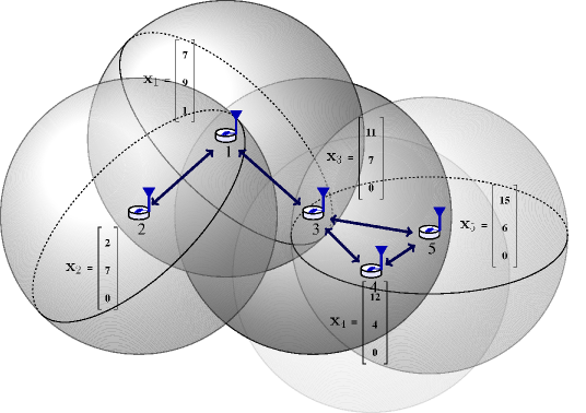
Figure 1: Sensor nodes deployed to measure not only environment information but also their pairwise distances. The observed distances are represented by two-sided arrows. The shadow spheres represent the radio communication range of the sensor nodes.

Second and more important problem is that the data center does not have enough distance information to identify the locations of sensor nodes. For various reasons, such as the power outage of a sensor node or the limitation of radio communication range, only small number of distance information is available at the data center. This situation can also occur in the hierarchical or relay-based IoT networks where only intermediate or cluster head node sends the distance information to the data center. Also, in the vehicular networks it might not be possible to measure the distance of all adjacent vehicles when a vehicle is located at the dead zone. Similar behavior can also be observed in underwater acoustic communication environments. To illustrate this scenario, we depict a simple network consisting of five sensor nodes in Fig. 1. We see that only a small number of pairwise distances are measured, and hence there are many unknown entries in the observation matrix $\mathbf{D}_{o}$:

$$\mathbf{D}_{o}=\left[\begin{array}[]{ccccccccccccccccccc}0&d_{12}^{2}&d_{13}^{2}&?&?\\ d_{21}^{2}&0&?&?&?\\ d_{31}^{2}&?&0&d_{34}^{2}&d_{35}^{2}\\ ?&?&d_{43}^{2}&0&d_{45}^{2}\\ ?&?&d_{53}^{2}&d_{54}^{2}&0\\ \end{array}\right],$$

where the question mark $?$ indicates unknown entries of $\mathbf{D}$. In finding out the node location using the observed matrix $\mathbf{D}_{o}$, multidimensional scaling (MDS) technique has been employed [10]. In a nutshell, MDS reconstructs the Euclidean distance matrix using the shortest path algorithm and then computes the node locations using a truncated eigendecomposition. Semidefinite programming (SDP) technique using a convex relaxation of nonconvex quadratic constraints of the node locations has also been used to this [14, 15]. However, SDP-based techniques are computationally expensive since the computational complexity depends heavily on the problem size [15].

As an alternative approach, matrix completion techniques reconstructing the Euclidean distance matrix $\mathbf{D}$ using partially observed entries have been proposed in recent years[16, 17, 18, 19, 20]. In general, one cannot recover the original matrix from a knowledge of a subset of its entries since there are infinitely many completion options for the unknown entries. However, if a matrix is low-rank, then it can be recovered from the partial observation matrix [16]. Since the rank of the Euclidean distance matrix $\mathbf{D}$ in the $k$-dimensional Euclidean space is at most $k+2$ ($k=2$ or $3$) [21], it can be readily modeled as a low-rank matrix. The problem to recover a low-rank matrix $\mathbf{D}$ from the small number of known entries can be expressed as

$$\begin{matrix}\min\limits_{\widetilde{\mathbf{D}}\>\in\>\mathbb{R}^{n\times n}}&\frac{1}{2}\|\mathcal{P}_{E}(\widetilde{\mathbf{D}})-\mathcal{P}_{E}(\mathbf{D}_{o})\|_{F}^{2},\\ \text{s.t.}&\text{rank}(\widetilde{\mathbf{D}})\leq k+2,\end{matrix}$$ (1)

where $\mathcal{P}_{E}$ is the sampling operator given by

$$[\mathcal{P}_{E}(\mathbf{A})]_{ij}=\left\{\begin{matrix}A_{ij}&\text{if }(i,j)\in E\\ 0&\text{otherwise}.\end{matrix}\right.$$

In the RSSI-based distance model, for example, $E=\{(i,j):\|\mathbf{x}_{i}-\mathbf{x}_{j}\|_{2}\leq r\}$ would be the set of observed indices for a given radio communication range $r$. Note that this problem is robust to the observation error and noise since it uses the Frobenius norm-based cost function. Also, this approach is good fit for the situation where the rank constraint is known in a priori, which is true in our case. In recent years, various approaches to find a solution of (1) have been suggested. In [16], the nuclear norm minimization (NNM) has been proposed. In [17], a singular value thresholding (SVT) technique that shrinks the number of singular values and as a result ensures the low rank structure of the output matrix has been proposed. As extensions of SVT technique, the augmented Lagrange multiplier (ALM) and accelerated proximal gradient (APG) algorithms have also been proposed in [18] and [22].

An aim of this paper is to propose a Euclidean distance matrix completion technique for the IoT network localization. In our approach, we express the Euclidean distance matrix $\mathbf{D}$ as a function of the low rank positive semidefinite (PSD) matrix. Since the set of these matrices forms a Riemannian manifold in which the notation of differentiability can be defined, we can recycle, after a proper modification, an algorithm in the Euclidean space. In order to solve the problem (1), we propose a modified conjugate gradient algorithm, referred to as localization in Riemannian manifold using conjugate gradient (LRM-CG). The main contributions of this paper are as follows:

• We propose a matrix completion-based IoT network localization algorithm called LRM-CG. Our numerical and simulation results demonstrate that LRM-CG can exactly recover the Euclidean distance matrix from partial measurements, achieving MSE $\leq 10^{-5}$ using 40% of measurements (see Subsection V-B).

• We propose an extension of LRM-CG to cope with the scenario in which the observed pairwise distances are contaminated by the outliers. By modeling outliers as a sparse matrix and then adding a regularization term of the outlier matrix into the Frobenius norm-based problem, we can effectively control the outliers. From simulation results, we observe that the extended LRM-CG is effective in handling the outliers, achieving mean square localization error being less than 0.5m up to 20% outlier ratio (see Subsection V-C).

We briefly summarize notations used in this paper. $<\boldsymbol{\beta}_{1},\boldsymbol{\beta}_{2}>$ is the inner product between $\boldsymbol{\beta}_{1}$ and $\boldsymbol{\beta}_{2}$, i.e., $<\boldsymbol{\beta}_{1},\boldsymbol{\beta}_{2}>=\text{tr}(\boldsymbol{\beta}_{1}^{T}\boldsymbol{\beta}_{2})$. $\text{diag}(\mathbf{A})$ is the vector formed by the main diagonal of a matrix $\mathbf{A}$. $\text{Sym}(\mathbf{A})$ and $\text{Skew}(\mathbf{A})$ are the matrices formed by $\text{Sym}(\mathbf{A})=\frac{1}{2}(\mathbf{A}+\mathbf{A}^{T})$ and $\text{Skew}(\mathbf{A})=\frac{1}{2}(\mathbf{A}-\mathbf{A}^{T})$ for any square matrix $\mathbf{A}$, respectively. Note that $\mathbf{A}=\text{Sym}(\mathbf{A})+\text{Skew}(\mathbf{A})$. $\text{eye}(\mathbf{a})$ is the diagonal matrix formed by $\mathbf{a}$. For an orthogonal matrix $\mathbf{Q}\in\mathbb{R}^{n\times k}$ with $n\textgreater k$, we define its orthogonal complement $\mathbf{Q}_{\perp}\in\mathbb{R}^{n\times(n-k)}$ such that $\left[\begin{array}[]{ccccccccccccccccccc}\mathbf{Q}&\mathbf{Q}_{\perp}\\ \end{array}\right]$ forms an orthonormal matrix. Given a function $f:\mathbf{Y}\in\mathbb{R}^{n\times n}\rightarrow f(\mathbf{Y})\in\mathbb{R}$, $\nabla_{\mathbf{Y}}f(\mathbf{Y})$ is the Euclidean gradient of $f(\mathbf{Y})$ with respect to $\mathbf{Y}$, i.e., $\left[\nabla_{\mathbf{Y}}f(\mathbf{Y})\right]_{ij}=\frac{\partial f(\mathbf{Y})}{\partial y_{ij}}$. For a given matrix $\mathbf{A}=\left[\begin{array}[]{ccccccccccccccccccc}\mathbf{a}_{1}&\mathbf{a}_{2}&\cdots&\mathbf{a}_{n}\\ \end{array}\right]\in\mathbb{R}^{n\times n}$, the vectorization of $\mathbf{A}$, denoted by $\text{vec}(\mathbf{A})$, is defined as $\text{vec}(\mathbf{A})=\left[\begin{array}[]{ccccccccccccccccccc}\mathbf{a}_{1}^{T}&\mathbf{a}_{2}^{T}&\cdots&\mathbf{a}_{n}^{T}\\ \end{array}\right]^{T}$. $\{\mathbf{e}_{i}\}_{i=1}^{n}$ are the $n\times 1$ standard basis vectors of $\mathbb{R}^{n}$. $\mathbf{A}\odot\mathbf{B}$ is the Hadamard product of two matrices $\mathbf{A}$ and $\mathbf{B}$. $\mathbf{1}=\left[\begin{array}[]{ccccccccccccccccccc}1&1&\cdots&1\\ \end{array}\right]^{T}$ is all-ones vector.

II The LRM-CG Algorithm

In this section, we present the proposed LRM-CG algorithm. By exploiting the smooth Riemannian manifold structure of the set of the low-rank symmetric PSD matrices, we formulate the matrix completion problem (1) as an unconstrained optimization problem on the smooth Riemannian manifold. Roughly speaking, smooth manifold is a generalization of the Euclidean space on which a notion of differentiability exists. For more rigorous definition, see, e.g., [23]. A smooth manifold together with an inner product, often called a Riemannian metric, forms a smooth Riemannian manifold. Since the smooth Riemannian manifold is a differentiable structure equipped with an inner product, we can use various ingredients such as Riemannian gradient, Hessian matrix, exponential map, and parallel translation, for solving optimization problems with quadratic cost function [23]. Therefore, optimization techniques in the Euclidean vector space (e.g., steepest descent, Newton method, conjugate gradient method) can be readily extended to solve a problem in the smooth Riemannian manifold.

II-A Problem Model

We consider the problem of $n$ sensor nodes distributed in the $k$-dimensional Euclidean space. Let $\mathbf{x}_{i}$ be the coordinate vector of the $i$-th sensor $(1\leq i\leq n)$ and $\mathbf{X}=[\mathbf{x}_{1}\ \mathbf{x}_{2}\ \cdots\ \mathbf{x}_{n}]^{T}$. Then, the distance $d_{ij}$ between the $i$-th and $j$-th sensors is given by $d_{ij}^{2}=\|\mathbf{x}_{i}-\mathbf{x}_{j}\|_{2}^{2}=\mathbf{x}_{i}^{T}\mathbf{x}_{i}+\mathbf{x}_{j}^{T}\mathbf{x}_{j}-2\mathbf{x}_{i}^{T}\mathbf{x}_{j}$, and thus the Euclidean distance matrix $\mathbf{D}$ satisfies

$$\mathbf{D}=g(\mathbf{XX}^{T}),$$ (2)

where $g(\mathbf{XX}^{T})=2\text{Sym}(\text{diag}(\mathbf{XX}^{T})\mathbf{1}^{T}-\mathbf{XX}^{T})$. In the example illustrated in Fig. 1, we have

$$\mathbf{X} =\left[\begin{array}[]{ccccccccccccccccccc}\mathbf{x}_{1}&\mathbf{x}_{2}&\mathbf{x}_{3}&\mathbf{x}_{4}&\mathbf{x}_{5}\\ \end{array}\right]^{T}$$

$$=\left[\begin{array}[]{ccccccccccccccccccc}7&2&11&12&15\\ 9&7&7&4&6\\ 1&0&0&0&0\\ \end{array}\right]^{T},$$

and

$$\mathbf{D}=g(\mathbf{XX}^{T})=\left[\begin{array}[]{ccccccccccccccccccc}0&30&21&51&74\\ 30&0&81&109&170\\ 21&81&0&10&17\\ 51&109&10&0&13\\ 74&170&17&13&0\\ \end{array}\right].$$

The problem to identify the node locations from a partial observation of $\mathbf{D}$ is formulated as

$$\begin{matrix}\min\limits_{\widetilde{\mathbf{X}}\>\in\>\mathbb{R}^{n\times k}}&\frac{1}{2}\|\mathcal{P}_{E}(g(\widetilde{\mathbf{X}}\widetilde{\mathbf{X}}^{T}))-\mathcal{P}_{E}(\mathbf{D}_{o})\|_{F}^{2}.\end{matrix}$$ (3)

When $n$ nodes ($n\geq k$) are distributed in $k$-dimensional Euclidean space, $\text{rank}(\mathbf{D})\leq k+2$ [14, 21]. Incorporating this constraint, we have

$$\begin{matrix}\min\limits_{\widetilde{\mathbf{D}}\>\in\>\mathbb{R}^{n\times n}}&\frac{1}{2}\|\mathcal{P}_{E}(\widetilde{\mathbf{D}})-\mathcal{P}_{E}(\mathbf{D}_{o})\|_{F}^{2},\\ \text{s.t.}&\text{rank}(\widetilde{\mathbf{D}})\leq k+2.\end{matrix}$$ (4)

Here, we use $\widetilde{\mathbf{X}}$ and $\widetilde{\mathbf{D}}$ as the optimization variables of the problems (3) and (4), respectively, to differentiate them from the true coordinate matrix $\mathbf{X}$ and the true distance matrix $\mathbf{D}$. In order to suppress the effect of large magnitude errors, we can incorporate a weight matrix $\mathbf{W}$ into (4). Thus,

$$\begin{matrix}\min\limits_{\widetilde{\mathbf{D}}\>\in\>\mathbb{R}^{n\times n}}&\frac{1}{2}\|\mathbf{W}\odot(\mathcal{P}_{E}(\widetilde{\mathbf{D}})-\mathcal{P}_{E}(\mathbf{D}_{o}))\|_{F}^{2},\\ \text{s.t.}&\text{rank}(\widetilde{\mathbf{D}})\leq k+2,\end{matrix}$$ (5)

where $w_{ij}$ is the $(i,j)$-th entry of $\mathbf{W}$ satisfying $w_{ij}\textgreater 0$ for $(i,j)\in E$ and zero otherwise. Noting that $\widetilde{\mathbf{D}}=g(\mathbf{Y})$ for a PSD matrix $\mathbf{Y}$, we further have

$$\begin{matrix}\min\limits_{\mathbf{Y}\>\in\>\mathcal{Y}}&\frac{1}{2}\|\mathbf{W}\odot(\mathcal{P}_{E}(g(\mathbf{Y}))-\mathcal{P}_{E}(\mathbf{D}_{o}))\|_{F}^{2},\end{matrix}$$ (6)

where $\mathcal{Y}=\{\widetilde{\mathbf{X}}\widetilde{\mathbf{X}}^{T}:\widetilde{\mathbf{X}}\in\mathbb{R}^{n\times k}\}$.

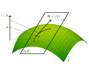
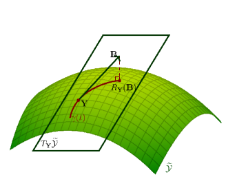
Figure 2: Illustration of (a) the tangent space $T_{\mathbf{Y}}\widetilde{\mathcal{Y}}$ and (b) the retraction operator $R_{\mathbf{Y}}$ at a point $\mathbf{Y}$ in the embedded manifold $\widetilde{\mathcal{Y}}$.

When the nodes are randomly distributed in $k$-dimensional Euclidean space, rank of the location matrix $\mathbf{X}$ is $k$ almost surely. Thus, we can strengthen the constraint set from $\mathcal{Y}$ to $\widetilde{\mathcal{Y}}=\{\widetilde{\mathbf{X}}\widetilde{\mathbf{X}}^{T}:\widetilde{\mathbf{X}}\in\mathbb{R}^{n\times k},\>\text{rank}(\widetilde{\mathbf{X}})=k\}$, and thus

$$\begin{matrix}\min\limits_{\mathbf{Y}\>\in\>\widetilde{\mathcal{Y}}}&\frac{1}{2}\|\mathbf{W}\odot(\mathcal{P}_{E}(g(\mathbf{Y}))-\mathcal{P}_{E}(\mathbf{D}_{o}))\|_{F}^{2},\end{matrix}$$ (7)

In the sequel, we denote $f(\mathbf{Y})=\frac{1}{2}\|\mathbf{W}\odot(\mathcal{P}_{E}(g(\mathbf{Y}))-\mathcal{P}_{E}(\mathbf{D}_{o}))\|_{F}^{2}$ for notational simplicity. Once the solution $\mathbf{Y}^{\ast}$ of the problem (7) is obtained, we can recover the node location using the eigen-decomposition of $\mathbf{Y}^{\ast}$ (see Subsection II-C for details).

II-B Optimization over Riemannian Manifold

Let $\mathcal{S}=\{\mathbf{S}\in\mathbb{R}^{n\times k}:\mathbf{S}^{T}\mathbf{S}=\mathbf{I}_{k}\}$ and $\mathcal{L}=\{\text{eye}([\begin{matrix}\lambda_{1}&\cdots&\lambda_{k}\end{matrix}]^{T}):\lambda_{1}\geq\lambda_{2}\geq\cdots\geq\lambda_{k}\textgreater 0\}$. Then, for given $\mathbf{T}\in\widetilde{\mathcal{Y}}$, we can express $\mathbf{T}=\mathbf{S}\boldsymbol{\Gamma}\mathbf{S}^{T}$ using the eigenvalue decomposition and thus

$$\widetilde{\mathcal{Y}}=\{\mathbf{S}\boldsymbol{\Gamma}\mathbf{S}^{T}:\mathbf{S}\in\mathcal{S},\boldsymbol{\Gamma}\in\mathcal{L}\},$$ (8)

where $\widetilde{\mathcal{Y}}$ is a smooth Riemannian manifold [25, Ch.5]. Our approach to solve the problem in a smooth Riemannian manifold is beneficial in two major respects: First, one can easily compute the gradient of the cost function in (7) using the matrix calculus. Second, one can extend techniques in the Euclidean space to solve the problem (7).

Since our work relies to a large extent on properties and operators of differential geometry, we briefly introduce tools and ingredients to describe the proposed algorithm. Since $\widetilde{\mathcal{Y}}$ is an embedded manifold in the Euclidean space $\mathbb{R}^{n\times n}$, its tangent spaces are determined by the derivative of its curves, where the curve $\gamma$ of $\widetilde{\mathcal{Y}}$ is a mapping from $\mathbb{R}$ to $\widetilde{\mathcal{Y}}$. Put it formally, for a given point $\mathbf{Y}=\mathbf{Q}\boldsymbol{\Lambda}\mathbf{Q}^{T}\in\widetilde{\mathcal{Y}}$, the tangent space of $\widetilde{\mathcal{Y}}$ at $\mathbf{Y}$, denoted $T_{\mathbf{Y}}\widetilde{\mathcal{Y}}$, is defined as $T_{\mathbf{Y}}\widetilde{\mathcal{Y}}=\{\gamma^{\prime}(0):\gamma\text{ is a curve in }\widetilde{\mathcal{Y}},\gamma(0)=\mathbf{Y}\}$ (see Fig. 2). The tangent space $T_{\mathbf{Y}}\widetilde{\mathcal{Y}}$ can be expressed as [26]

$$T_{\mathbf{Y}}\widetilde{\mathcal{Y}} = \left\{\left[\begin{matrix}\mathbf{Q}&\mathbf{Q}_{\perp}\end{matrix}\right]\left[\begin{matrix}\mathbf{C}_{1}&\mathbf{C}_{2}^{T}\\ \mathbf{C}_{2}&\mathbf{0}\end{matrix}\right]\left[\begin{matrix}\mathbf{Q}^{T}\\ \mathbf{Q}_{\perp}^{T}\end{matrix}\right]:\right.$$ (9)

$$\left.\mathbf{C}_{1}^{T}=\mathbf{C}_{1}\in\mathbb{R}^{k\times k},\mathbf{C}_{2}\in\mathbb{R}^{(n-k)\times k}\right\}.$$

A metric on the tangent space $T_{\mathbf{Y}}\widetilde{\mathcal{Y}}$ is defined as the matrix inner product $<\mathbf{B}_{1},\mathbf{B}_{2}>=\text{tr}(\mathbf{B}_{1}^{T}\mathbf{B}_{2})$ between two tangent components $\mathbf{B}_{1},\mathbf{B}_{2}\in T_{\mathbf{Y}}\widetilde{\mathcal{Y}}$. Next, we define the orthogonal projection of a matrix $\mathbf{A}$ onto the tangent space $T_{\mathbf{Y}}\widetilde{\mathcal{Y}}$, which will be used to find the closed-form expression of Riemannian gradient in Subsection II-C.

Definition II.1.

The orthogonal projection onto $T_{\mathbf{Y}}\widetilde{\mathcal{Y}}$ is a mapping $P_{T_{\mathbf{Y}}\widetilde{\mathcal{Y}}}:\mathbb{R}^{n\times n}\rightarrow T_{\mathbf{Y}}\widetilde{\mathcal{Y}}$ such that for a given matrix $\mathbf{A}_{1}\in\mathbb{R}^{n\times n}$, $<\mathbf{A}_{1}-P_{T_{\mathbf{Y}}\widetilde{\mathcal{Y}}}(\mathbf{A}_{1}),\mathbf{A}_{2}>=0$ for all $\mathbf{A}_{2}\in T_{\mathbf{Y}}\widetilde{\mathcal{Y}}$.

For a given matrix $\mathbf{A}_{1}$, orthogonal projection $P_{T_{\mathbf{Y}}\widetilde{\mathcal{Y}}}(\mathbf{A}_{1})$ of $\mathbf{A}_{1}$ onto the tangent space $T_{\mathbf{Y}}\widetilde{\mathcal{Y}}$ is [26]

$$P_{T_{\mathbf{Y}}\widetilde{\mathcal{Y}}}(\mathbf{A}_{1})=\mathbf{P}_{\mathbf{Q}}\text{Sym}(\mathbf{A}_{1})+\text{Sym}(\mathbf{A}_{1})\mathbf{P}_{\mathbf{Q}}-\mathbf{P}_{\mathbf{Q}}\text{Sym}(\mathbf{A}_{1})\mathbf{P}_{\mathbf{Q}},$$ (10)

where $\mathbf{P}_{\mathbf{Q}}=\mathbf{QQ}^{T}$.

In order to express the concept of moving in the direction of a tangent space while staying on the manifold, an operation called retraction is used. As illustrated in Fig. 2(b), the retraction operation is a mapping from $T_{\mathbf{Y}}\widetilde{\mathcal{Y}}$ to $\widetilde{\mathcal{Y}}$ that preserves the gradient at $\mathbf{Y}$ [27, Definition 4.1.1].

Definition II.2.

The retraction $R_{\mathbf{Y}}(\mathbf{B})$ of a matrix $\mathbf{B}\in T_{\mathbf{Y}}\widetilde{\mathcal{Y}}$ onto $\widetilde{\mathcal{Y}}$ is defined as

$$R_{\mathbf{Y}}(\mathbf{B})=\arg\min\limits_{\mathbf{Z}\in\widetilde{\mathcal{Y}}}\|\mathbf{Y}+\mathbf{B}-\mathbf{Z}\|_{F}.$$ (11)

In obtaining the closed form expression of $R_{\mathbf{Y}}(\mathbf{B})$, an operator $\mathcal{W}_{k}$ keeping $k$ largest positive eigenvalues of a matrix, referred to as eigenvalue selection operator, is needed. Since the projection $R_{\mathbf{Y}}(\mathbf{B})$ is an element of $\widetilde{\mathcal{Y}}$, $R_{\mathbf{Y}}(\mathbf{B})$ should be a symmetric PSD matrix with rank $k$. Thus, for a given square matrix $\mathbf{A}$, we are interested only in the symmetric part $Sym(\mathbf{A})$. If we denote the eigenvalue decomposition (EVD) of this as $Sym(\mathbf{A})=\mathbf{P}\boldsymbol{\Sigma}\mathbf{P}^{T}$ and the $k$ topmost eigenvalues of this as $\sigma_{1}\geq\sigma_{2}\geq\cdots\geq\sigma_{k}$ , then $\mathcal{W}_{k}(\mathbf{A})$ is defined as

$$\mathcal{W}_{k}(\mathbf{A})=\mathbf{P}\boldsymbol{\Sigma}_{k}\mathbf{P}^{T},$$ (12)

where $\boldsymbol{\Sigma}_{k}=\text{eye}\left(\left[\begin{array}[]{ccccccccccccccccccc}\sigma_{1}&...&\sigma_{k}&0&...&0\\ \end{array}\right]^{T}\right)$. Using this eigenvalue selection operator $\mathcal{W}_{k}$, we can obtain an elegant expression of $R_{\mathbf{Y}}(\mathbf{B})$.

Theorem II.3 (Proposition 6 [27]).

The retraction $R_{\mathbf{Y}}(\mathbf{B})$ of $\mathbf{B}\in T_{\mathbf{Y}}\widetilde{\mathcal{Y}}$ can be expressed as

$$R_{\mathbf{Y}}(\mathbf{B})=\mathcal{W}_{k}(\mathbf{Y}+\mathbf{B}).$$ (13)

Finally, to develop the conjugate gradient algorithm over the Riemannian manifold $\widetilde{\mathcal{Y}}$, we need the Euclidean gradient of the cost function $f(\mathbf{Y})$.

Theorem II.4.

Euclidean gradient $\nabla_{\mathbf{Y}}f(\mathbf{Y})$ of $f(\mathbf{Y})$ with respect to $\mathbf{Y}$ is

$$\nabla_{\mathbf{Y}}f(\mathbf{Y})=2\text{eye}(\text{Sym}(\mathbf{R})\mathbf{1})-2\text{Sym}(\mathbf{R}),$$ (14)

where $\mathbf{R}=\mathbf{W}\odot\mathbf{W}\odot(\mathcal{P}_{E}(g(\mathbf{Y}))-\mathcal{P}_{E}(\mathbf{D}_{o}))$.

Proof.

See Appendix A. ∎

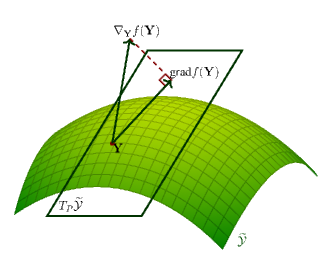
Figure 3: Riemannian gradient $\text{grad}f(\mathbf{Y})$ is defined as the projection of the Euclidean gradient $\nabla_{\mathbf{Y}}f(\mathbf{Y})$ onto the tangent space $T_{\mathbf{Y}}\widetilde{\mathcal{Y}}$ while the Euclidean gradient is a direction for which the cost function is reduced most in $\mathbb{R}^{n\times n}$, Riemannian gradient is the direction for which the cost function is reduced most in the tangent space $T_{\mathbf{Y}}\widetilde{\mathcal{Y}}$.

II-C Localization in Riemannian Manifold Using Conjugate Gradient (LRM-CG)

In order to solve the problem (7), we basically use the conjugate gradient (CG) algorithm. CG algorithm is widely used to solve the sparse symmetric positive definite linear systems [28]. Main advantage of the CG algorithm is that the solution can be found in a finite number of searching steps. This is because the conjugate direction is designed such that it is conjugate to the previous directions and also the gradient of the cost function.

First, noting that $\mathcal{P}_{E}$ and $g$ are linear mappings, one can easily show that

$$f(\mathbf{Y}) = \frac{1}{2}\|\mathbf{W}\odot(\mathcal{P}_{E}(g(\mathbf{Y}))-\mathcal{P}_{E}(\mathbf{D}_{o}))\|_{F}^{2}$$ (15)

$$= \frac{1}{2}\|\mathbf{W}\odot(\mathcal{P}_{E}(g(\sum\limits_{i,j}y_{ij}\mathbf{e}_{i}\mathbf{e}_{j}^{T}))-\mathcal{P}_{E}(\mathbf{D}_{o}))\|_{F}^{2}$$

$$= \frac{1}{2}\|\mathbf{W}\odot(\sum\limits_{i,j}y_{ij}\mathcal{P}_{E}(g(\mathbf{e}_{i}\mathbf{e}_{j}^{T}))-\mathcal{P}_{E}(\mathbf{D}_{o}))\|_{F}^{2}$$

$$\begin{subarray}{c}(a)\\ =\end{subarray} \frac{1}{2}\|\text{vec}(\mathbf{W})\circ(\sum\limits_{i,j}y_{ij}\text{vec}\left(\mathcal{P}_{E}(g(\mathbf{e}_{i}\mathbf{e}_{j}^{T}))\right)$$

$$-\text{vec}(\mathcal{P}_{E}(\mathbf{D}_{o})))\|_{2}^{2}$$

$$\begin{subarray}{c}(b)\\ =\end{subarray} \frac{1}{2}\|\mathbf{A}\text{vec}(\mathbf{Y})-\mathbf{b}\|_{2}^{2},$$

where (a) is because $\|\mathbf{M}\|_{F}=\|\text{vec}(\mathbf{M})\|_{2}$, (b) follows from $\text{vec}(\mathbf{Y})=\left[\begin{array}[]{ccccccccccccccccccc}y_{11}&y_{21}&\cdots&y_{nn}\\ \end{array}\right]^{T}$, $\mathbf{b}=\text{vec}(\mathbf{W}\odot\mathcal{P}_{E}(\mathbf{D}_{o}))$, and $\mathbf{A}$ formed by column vectors $\text{vec}\left(\mathbf{W}\odot\mathcal{P}_{E}(g(\mathbf{e}_{i}\mathbf{e}_{j}^{T}))\right)$.

In (15), we see that the cost function $f(\mathbf{Y})$ has the quadratic form of a sparse symmetric positive definite system, and thus the CG algorithm can be readily used to solve the problem. The update equation of the conventional CG algorithm in the Euclidean space is

$$\mathbf{Y}_{i+1}=\mathbf{Y}_{i}+\alpha_{i}\mathbf{P}_{i},$$ (16)

where $\alpha_{i}$ is the stepsize and $\mathbf{P}_{i}$ is the conjugate direction. The stepsize $\alpha_{i}$ is chosen by the line minimization technique (e.g., Armijo’s rule [28]) and the search direction $\mathbf{P}_{i}$ of the CG algorithm is chosen as a linear combination of the gradient and the previous search direction to generate a direction conjugate to the previous ones. In doing so, one can avoid unnecessary searching of directions that have been searched over and thus achieve the speedup of the algorithm [28].

Algorithm 1: LRM-CG algorithm

1 Input: $\mathbf{D}_{o}$: the observed matrix,       $\mathbf{W}$: the weight matrix,       $\mathcal{P}_{E}$: the sampling operator,       $\epsilon$: tolerance,       $\mu\in(0\>\>\>1)$: given constant,       $T$: number of iterations. 2 Output: $\widehat{\mathbf{X}}$: node location matrix 3 Initialize: $i=1$,          $\mathbf{Y}_{1}\in\widetilde{\mathcal{Y}}$: initial matrix,          $\mathbf{P}_{1}$: initial conjugate direction. 4 While $i\leq T$ do 5    $\mathbf{R}_{i}=\mathbf{W}\odot\mathbf{W}\odot(\mathcal{P}_{E}(g(\mathbf{Y}_{i}))-\mathcal{P}_{E}(\mathbf{D}_{o}))$ // Generate residual matrix 6    $\nabla_{\mathbf{Y}}f(\mathbf{Y}_{i})=2\text{eye}(\text{Sym}(\mathbf{R}_{i})\mathbf{1})-2\mathbf{R}_{i}$ // Compute Euclidean gradient 7    $\text{grad}f(\mathbf{Y}_{i})=P_{T_{\mathbf{Y}_{i}}\widetilde{\mathcal{Y}}}(\nabla_{\mathbf{Y}}f(\mathbf{Y}_{i}))$ // Compute Riemannian gradient 8    $\mathbf{H}_{i}=\text{grad}f(\mathbf{Y}_{i})-P_{T_{\mathbf{Y}_{i}}\widetilde{\mathcal{Y}}}(\text{grad}f(\mathbf{Y}_{i-1}))$ 9    $h=<\mathbf{P}_{i},\mathbf{H}_{i}>$ 10    $\beta_{i}=\frac{1}{h^{2}}<h\mathbf{H}_{i}-2\mathbf{P}_{i}\|\mathbf{H}_{i}\|_{F}^{2},\text{grad}f(\mathbf{Y}_{i})>$ // Compute CG coefficient 11    $\mathbf{P}_{i}=-\text{grad}f(\mathbf{Y}_{i})+\beta_{i}P_{T_{\mathbf{Y}_{i}}\widetilde{\mathcal{Y}}}(\mathbf{P}_{i-1})$ // Compute conjugate direction 12    Find a stepsize $\alpha_{i}\textgreater 0$ such that // Perform Armijo’s line search     $f(\mathbf{Y}_{i})-f(R_{\mathbf{Y}_{i}}(\alpha_{i}\mathbf{P}_{i}))\geq-\mu\alpha_{i}<\text{grad}f(\mathbf{Y}_{i}),\mathbf{P}_{i}>$ 13    $\mathbf{Y}_{i+1}=R_{\mathbf{Y}_{i}}(\alpha_{i}\mathbf{P}_{i})$ // Perform retraction 14    $\mathbf{D}_{i+1}=g(\mathbf{Y}_{i+1})$ // Compute updated Euclidean distance matrix 15    If $\|\mathbf{W}\odot(\mathcal{P}_{E}(\mathbf{D}_{i+1})-\mathcal{P}_{E}(\mathbf{D}_{o}))\|_{F}\textless\epsilon$ then 16     Exit from while loop 17    End If 18    Obtain $\mathbf{Q}$ and $\boldsymbol{\Lambda}$ using the eigendecomposition     $\mathbf{Y}_{i+1}=\mathbf{Q}\boldsymbol{\Lambda}\mathbf{Q}^{T}$ 19    $\widehat{\mathbf{X}}=\mathbf{Q}\boldsymbol{\Lambda}^{1/2}$ // Find updated locations of sensor nodes 20    $i=i+1$ 21 End While

Since we consider the optimization problem over the Riemannian manifold $\widetilde{\mathcal{Y}}$, the conjugate direction $\mathbf{P}_{i}$ should lie on the tangent space. To make sure that the update point $\mathbf{Y}_{i+1}$ lies on the manifold, we need a retraction operation. The update equation after applying the retraction operation is

$$\mathbf{Y}_{i+1} = R_{\mathbf{Y}_{i}}(\alpha_{i}\mathbf{P}_{i})=\mathcal{W}_{k}(\mathbf{Y}_{i}+\alpha_{i}\mathbf{P}_{i}).$$ (17)

As observed in Theorem 13, the eigenvalue selection operator $\mathcal{W}_{k}$ guarantees that the updated point $\mathbf{Y}_{i+1}$ lies on the manifold.

We next consider the conjugate direction $\mathbf{P}_{i}$ of LRM-CG. In the conventional nonlinear CG algorithm, conjugate direction $\mathbf{P}_{i}$ is updated as

$$\mathbf{P}_{i}=-\nabla_{\mathbf{Y}}f(\mathbf{Y}_{i})+\beta_{i}\mathbf{P}_{i-1},$$ (18)

where $\beta_{i}$ is the conjugate update parameter. Since we optimize over the Riemannian manifold $\widetilde{\mathcal{Y}}$, conjugate direction in (18) needs to be modified. First, we need to use the Riemannian gradient of $f(\mathbf{Y})$ instead of the Euclidean gradient $\nabla_{\mathbf{Y}}f(\mathbf{Y})$ since we need to find the search direction on the tangent space of $\widetilde{\mathcal{Y}}$. Riemannian gradient, denoted $\text{grad}f(\mathbf{Y})$, is distinct from $\nabla_{\mathbf{Y}}f(\mathbf{Y})$ in the sense that it is defined on the tangent space $T_{\mathbf{Y}}\widetilde{\mathcal{Y}}$ (see Fig. 3). $\text{grad}f(\mathbf{Y})$ is given in the following lemma.

Lemma II.5 (Ch.3 [23]).

Riemannian gradient $\nabla_{\mathbf{Y}}f(\mathbf{Y})$ of $f(\mathbf{Y})$ with respect to $\mathbf{Y}$ is

$$\text{grad}f(\mathbf{Y})=P_{T_{\mathbf{Y}}\widetilde{\mathcal{Y}}}(\nabla_{\mathbf{Y}}f(\mathbf{Y})).$$ (19)

Second, since the Riemannian gradient $\text{grad}f(\mathbf{Y}_{i})$ and previous conjugate direction $\mathbf{P}_{i-1}$ lie on two different vector spaces $T_{\mathbf{Y}_{i}}\widetilde{\mathcal{Y}}$ and $T_{\mathbf{Y}_{i-1}}\widetilde{\mathcal{Y}}$, we need to project $\mathbf{P}_{i-1}$ onto the tangent space $T_{\mathbf{Y}_{i}}\widetilde{\mathcal{Y}}$ before performing a linear combination between of two. In view of this, the conjugate direction update equation of LRM-CG is

$$\mathbf{P}_{i}=-\text{grad}f(\mathbf{Y}_{i})+\beta_{i}P_{T_{\mathbf{Y}_{i}}\widetilde{\mathcal{Y}}}(\mathbf{P}_{i-1}).$$ (20)

In finding the stepsize $\alpha_{i}$ in (17), we use the Armijo’s rule ($\alpha_{i}\approx\min\limits_{\alpha\textgreater 0}f(\mathcal{W}_{k}(\mathbf{Y}_{i}+\alpha_{i}\mathbf{P}_{i})$ [28]), a widely used line search strategy.

Finally, when the output $\widehat{\mathbf{Y}}\in\widetilde{\mathcal{Y}}$ of LRM-CG is generated, the node location matrix $\widehat{\mathbf{X}}$ is recovered as

$$\widehat{\mathbf{X}}=\arg\min\limits_{\mathbf{X}}\|\widehat{\mathbf{Y}}-\mathbf{XX}^{T}\|_{F}.$$ (21)

Since $\widehat{\mathbf{Y}}\succeq 0$, we use the eigenvalue decomposition to find $\widehat{\mathbf{X}}$. In fact, by denoting $\widehat{\mathbf{Y}}=\mathbf{Q}\boldsymbol{\Lambda}\mathbf{Q}^{T}$ ($\mathbf{Q}\in\mathbb{R}^{n\times k}$ and $\boldsymbol{\Lambda}\in\mathbb{R}^{k\times k}$), we obtain the local locations of sensor nodes $\widehat{\mathbf{X}}=\mathbf{Q}\boldsymbol{\Lambda}^{1/2}$. Then, $\widehat{\mathbf{X}}$ is transformed into the true locations of nodes by the aid of anchor nodes [10, 8]. Specifically, we might need to find a rotation matrix $\mathbf{F}\in\mathbb{R}^{k\times k}$ and a translation vector $\mathbf{b}\in\mathbb{R}^{k}$ to transform $\widehat{\mathbf{X}}$ so that it would be matched with the true locations as

$$\mathbf{X}=\widehat{\mathbf{X}}\mathbf{F}+\mathbf{1b}^{T}.$$ (22)

Suppose that $\mathbf{x}_{1}$, $\mathbf{x}_{2}$, and $\mathbf{x}_{3}$ are the given anchor nodes in 2-dimensional Euclidean space ($k=2$). Since $\mathbf{x}_{1}^{T}=\widehat{\mathbf{x}}_{1}^{T}\mathbf{F}+\mathbf{b}^{T}$ and $\mathbf{b}^{T}=\mathbf{x}_{1}^{T}-\widehat{\mathbf{x}}_{1}^{T}\mathbf{F}$, we have

$$\mathbf{X}-\mathbf{1x}_{1}^{T} =(\widehat{\mathbf{X}}-\mathbf{1}\widehat{\mathbf{x}}_{1}^{T})\mathbf{F}+\mathbf{1}\widehat{\mathbf{x}}_{1}^{T}\mathbf{F}-\mathbf{1x}_{1}^{T}+\mathbf{1b}^{T}$$

$$=(\widehat{\mathbf{X}}-\mathbf{1}\widehat{\mathbf{x}}_{1}^{T})\mathbf{F}.$$ (23)

What remains is to find $\mathbf{F}$. Let $\mathbf{X}_{A}=\left[\begin{array}[]{ccccccccccccccccccc}\mathbf{x}_{2}-\mathbf{x}_{1}&\mathbf{x}_{3}-\mathbf{x}_{1}\\ \end{array}\right]^{T}$ and $\widehat{\mathbf{X}}_{A}=\left[\begin{array}[]{ccccccccccccccccccc}\widehat{\mathbf{x}}_{2}-\widehat{\mathbf{x}}_{1}&\widehat{\mathbf{x}}_{3}-\widehat{\mathbf{x}}_{1}\\ \end{array}\right]$ be the matrices associated to anchor nodes. Then, it is clear that $\mathbf{X}_{A}=\widehat{\mathbf{X}}_{A}\mathbf{F}$. Thus, we have $\mathbf{F}=\widehat{\mathbf{X}}_{A}^{\dagger}\mathbf{X}_{A}$.

The proposed LRM-CG algorithm is summarized in Algorithm 1.

II-D Computational Complexity

In this subsection, we analyze the computational complexity of LRM-CG in terms of the number of floating point operations (flops). As discussed, major operations in LRM-CG is to compute Euclidean gradient, Riemannian gradient, and the retraction operation.

First, in order to compute the Euclidean gradient $\nabla_{\mathbf{Y}}f(\mathbf{Y}_{i})$ in (14), we need to compute $\mathcal{P}_{E}(g(\mathbf{Y}_{i}))$, $\mathbf{R}_{i}=\mathbf{W}\odot\mathbf{W}\odot(\mathcal{P}_{E}(g(\mathbf{Y}_{i}))-\mathcal{P}_{E}(\mathbf{D}_{o}))$, and $2\text{eye}(\text{Sym}(\mathbf{R}_{i})\mathbf{1})-2\text{Sym}(\mathbf{R}_{i})$, which require $3|E|/2$, $3|E|/2$, and $\mathcal{O}(|E|)$ flops, respectively, where $|E|$ is the number of elements of $E$ defined in (1). Second, recalling that the Riemannian gradient $\text{grad}f(\mathbf{Y}_{i})$ is an orthogonal projection of $\nabla_{\mathbf{Y}}f(\mathbf{Y}_{i})$ onto the tangent space $T_{\mathbf{Y}_{i}}\widetilde{\mathcal{Y}}$, we need to estimate the computational complexity of the orthogonal projection operator $P_{T_{\mathbf{Y}_{i}}\widetilde{\mathcal{Y}}}$. By adopting the computational strategy in [26], we can express the Riemannian gradient as $\text{grad}f(\mathbf{Y}_{i})=\mathbf{Q}\mathbf{C}_{1}\mathbf{Q}^{T}+\mathbf{Q}\widetilde{\mathbf{C}}^{T}+\widetilde{\mathbf{C}}\mathbf{Q}^{T}$ where $\mathbf{C}_{1}\in\mathbb{R}^{k\times k}$, $\widetilde{\mathbf{C}}\in\mathbb{R}^{n\times k}$, and $\mathbf{Q}^{T}\widetilde{\mathbf{C}}=\mathbf{0}$, which requires $\mathcal{O}(k|E|+k^{2}n)$. Finally, the retraction operation is obtained via the eigenvalue selection operator $\mathcal{W}_{k}$ in (13) and this requires the EVD of $(\mathbf{Y}_{i}+\mathbf{P}_{i})$. In general, the computational complexity of the EVD for an $n\times n$ matrix is expressed as $\mathcal{O}(n^{3})$. However, by exploiting the symmetric structures of $\widetilde{\mathcal{Y}}$ and $T_{\mathbf{Y}_{i}}\widetilde{\mathcal{Y}}$, we can simplify the EVD operation (see [26] for details). Specifically, noting that $\mathbf{P}_{i}\in T_{\mathbf{Y}_{i}}\widetilde{\mathcal{Y}}$, we have

$$\mathbf{Y}_{i}+\mathbf{P}_{i} = \left[\begin{matrix}\mathbf{Q}&\mathbf{Q}_{c}\end{matrix}\right]\left[\begin{matrix}\boldsymbol{\Lambda}+\mathbf{C}_{1}&\mathbf{R}_{c}^{T}\\ \mathbf{R}_{c}&\mathbf{0}\end{matrix}\right]\left[\begin{matrix}\mathbf{Q}^{T}\\ \mathbf{Q}_{c}^{T}\end{matrix}\right]$$

$$= \left[\begin{matrix}\mathbf{Q}&\mathbf{Q}_{c}\end{matrix}\right]\textbf{K}\boldsymbol{\Lambda}^{{}^{\prime}}\textbf{K}^{T}\left[\begin{matrix}\mathbf{Q}^{T}\\ \mathbf{Q}_{c}^{T}\end{matrix}\right].$$

where $\mathbf{Q}_{c}\mathbf{R}_{c}$ is the QR-decomposition of an $n\times k$ matrix satisfying $\mathbf{Q}^{T}\mathbf{Q}_{c}=\mathbf{0}$, which requires $\mathcal{O}(k^{2}n+k^{3})$. Now the EVD of $(\mathbf{Y}_{i}+\mathbf{P}_{i})$ is simplified to the EVD of the $2k\times 2k$ matrix $\left[\begin{matrix}\boldsymbol{\Lambda}+\mathbf{C}_{1}&\mathbf{R}_{c}^{T}\\ \mathbf{R}_{c}&\mathbf{0}\end{matrix}\right]$, which requires only $\mathcal{O}(k^{3})$ flops. Also, the computation of $\left[\begin{matrix}\mathbf{Q}&\mathbf{Q}_{c}\end{matrix}\right]\textbf{K}$ requires $nk(4k-1)$ flops. As a result, the computational complexity of the retraction operation is $\mathcal{O}(k^{2}n)$.

In summary, the computational complexity of the proposed algorithm per iteration is $\mathcal{O}(k|E|+k^{2}n)$. Since $k=2$ or $3$ in our problem [21], the computational complexity per iteration can be expressed as $\mathcal{O}(|E|+n)$ flops.

III Convergence Analysis

In this section, we present the convergence analysis of the proposed LRM-CG algorithm. We show that under the extended Wolfe’s conditions, LRM-CG converges linearly to the original Euclidean distance matrix in the sampling space.

Definition III.1.

For a sequence of matrices $\{\mathbf{D}_{i}\}_{i=1}^{\infty}$, if $\lim\limits_{i\rightarrow\infty}\|\mathbf{D}_{i}-\mathbf{D}\|_{F}=0$, we say $\{\mathbf{D}_{i}\}_{i=1}^{\infty}$ converges to $\mathbf{D}$. Further, we say $\{\mathbf{D}_{i}\}_{i=1}^{\infty}$ converges linearly to $\mathbf{D}$ with convergent rate $\lambda$ if there exists $\lambda$ ($1\textgreater\lambda\geq 0$) satisfying

$$\lim\limits_{i\rightarrow\infty}\quad\frac{\|\mathbf{D}_{i+1}-\mathbf{D}\|_{F}}{\|\mathbf{D}_{i}-\mathbf{D}\|_{F}}=\lambda.$$

The minimal set of assumptions used for the analytical tractability are as follows:

• $f(\mathbf{Y}_{i})-f(R_{\mathbf{Y}_{i}}(\alpha_{i}\mathbf{P}_{i}))\geq-\tau\alpha_{i}<\text{grad}f(\mathbf{Y}_{i}),\mathbf{P}_{i}>$ for $\tau$ satisfying $0\textless\tau\textless 1/2$,

• $|<\text{grad}f(R_{\mathbf{Y}_{i}}(\alpha_{i}\mathbf{P}_{i})),\mathbf{P}_{i}>|\leq-\mu<\text{grad}f(\mathbf{Y}_{i}),\mathbf{P}_{i}>$ for $\mu$ satisfying $\tau\textless\mu\textless 1/2$,

• $c\|\text{grad}f(\mathbf{Y}_{i})\|_{F}\geq\|\nabla_{\mathbf{Y}}f(\mathbf{Y}_{i})\|_{F}$ for $c$ satisfying $c\textgreater 1$.

In essence, $\mathbf{A1}$ and $\mathbf{A2}$ can be considered as extensions of the strong Wolfe’s conditions [30, 31]. Note that if the stepsize $\alpha_{i}$ is chosen to be very small, then $\mathbf{Y}_{i+1}=R_{\mathbf{Y}_{i}}(\alpha_{i}\mathbf{P}_{i})\approx R_{\mathbf{Y}_{i}}(\mathbf{0})=\mathbf{Y}_{i}$, and thus $f(\mathbf{Y}_{i})-f(R_{\mathbf{Y}_{i}}(\alpha_{i}\mathbf{P}_{i}))\approx 0$ and $-\tau\alpha_{i}<\text{grad}f(\mathbf{Y}_{i}),\mathbf{P}_{i}>\approx 0$. In this case, A1 holds true approximately. However, there would be almost no update of $\mathbf{Y}_{i}$ so that the algorithm will converge extremely slowly. To circumvent this pathological scenario, we use A2, which is in essence an extension of the strong Wolfe’s condition for the Riemannian manifold. Under this assumption, $\alpha_{i}$ cannot be chosen to be very small since otherwise we have $R_{\mathbf{Y}_{i}}(\alpha_{i}\mathbf{P}_{i})\approx\mathbf{Y}_{i}$, and thus

$$|<\text{grad}f(R_{\mathbf{Y}_{i}}(\alpha_{i}\mathbf{P}_{i})),\mathbf{P}_{i}>| \approx|<\text{grad}f(\mathbf{Y}_{i}),\mathbf{P}_{i}>|$$

$$\geq-\mu<\text{grad}f(\mathbf{Y}_{i}),\mathbf{P}_{i}>,$$

which contradicts the assumption A2. The assumption A3 is needed to guarantee the global convergence of LRM-CG. We will discuss more on this in Remark III.5.

Our first main result, stating successful recovery condition at sampled entries, is formally described in the following theorem.

Theorem III.2 (strong convergence of LRM-CG).

Let $\{\mathbf{D}_{i}=g(\mathbf{Y}_{i})\}_{i=1}^{\infty}$ be the sequence of the matrices generated by LRM-CG and $\mathbf{D}$ be the original Euclidean distance matrix. Under $\mathbf{A1}$, $\mathbf{A2}$, and $\mathbf{A3}$, $\{\mathcal{P}_{E}(\mathbf{D}_{i})\}_{i=0}^{\infty}$ converges linearly to $\mathcal{P}_{E}(\mathbf{D})$.

Remark III.3 (strongly convergent condition in $\mathbb{R}^{n}$).

Note that $\lim\limits_{i\rightarrow\infty}\|\mathcal{P}_{E}(\mathbf{D}_{i})-\mathcal{P}_{E}(\mathbf{D})\|_{F}=0$ is equivalent to

$$\lim\limits_{i\rightarrow\infty}\|\nabla_{\mathbf{Y}}f(\mathbf{Y}_{i})\|_{F}=0.$$ (24)

This condition is often referred to as the strongly convergent condition of the nonlinear CG algorithms in the vector space. The equivalence can be established by the following sandwich lemma.

Lemma III.4.

$$2\|\mathcal{P}_{E}(\mathbf{D}_{i})-\mathcal{P}_{E}(\mathbf{D})\|_{F} \leq\|\nabla_{\mathbf{Y}}f(\mathbf{Y}_{i})\|_{F}$$

$$\leq(2\sqrt{n}+2)\|\mathcal{P}_{E}(\mathbf{D}_{i})-\mathcal{P}_{E}(\mathbf{D})\|_{F}.$$

Proof.

See Appendix B ∎

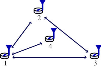
Figure 4: Suppose that the sensor node 4 is inside the triangle formed by three sensor nodes 1, 2, and 3. Then for a given $r$, it can be shown that $d_{14}\leq\max(d_{12},d_{13})$, and thus $P(d_{14}\leq r|d_{12}\leq r,d_{13}\leq r)=1$ which is not necessarily equivalent to $P(d_{14}\leq r)$.

Remark III.5.

Recently, an attempt has been made to extend the convergent analysis of the conventional CG algorithms (over the Euclidean space $\mathbb{R}^{n}$) to the Riemannian manifolds. In [31, Theorem 4.3], it has been shown that under certain assumption,

$$\lim\limits_{i\rightarrow\infty}\inf\|\text{grad}f(\mathbf{Y}_{i})\|_{F}=0.$$ (25)

One can observe that the Euclidean gradient $\nabla_{\mathbf{Y}}f(\mathbf{Y}_{i})$ is replaced by the Riemannian gradient $\text{grad}f(\mathbf{Y}_{i})$. Unfortunately, the convergence of the Riemannian gradient in (25) does not imply the convergence of Euclidean gradient in (24) because

$$\|\nabla_{\mathbf{Y}}f(\mathbf{Y}_{i})\|_{F}^{2}$$ (26)

$$= \|\mathcal{P}_{T_{\mathbf{Y}}\widetilde{\mathcal{Y}}}(\nabla_{\mathbf{Y}}f(\mathbf{Y}_{i}))\|_{F}^{2}+\|\mathcal{P}^{\perp}_{T_{\mathbf{Y}}\widetilde{\mathcal{Y}}}(\nabla_{\mathbf{Y}}f(\mathbf{Y}_{i}))\|_{F}^{2}$$

$$= \|\text{grad}f(\mathbf{Y}_{i})\|_{F}^{2}+\|\mathcal{P}^{\perp}_{T_{\mathbf{Y}}\widetilde{\mathcal{Y}}}(\nabla_{\mathbf{Y}}f(\mathbf{Y}_{i}))\|_{F}^{2},$$

where $\text{grad}f(\mathbf{Y}_{i})=\mathcal{P}_{T_{\mathbf{Y}}\widetilde{\mathcal{Y}}}(\nabla_{\mathbf{Y}}f(\mathbf{Y}_{i}))$ (see (19)). One can observe from this that the condition in (25) is not sufficient to guarantee (24), that is, one cannot guarantee $\lim\limits_{i\rightarrow\infty}\|\mathcal{P}_{E}(\mathbf{D}_{i})-\mathcal{P}_{E}(\mathbf{D})\|_{F}=0$ just from (25). However, by the introduction of A3, equivalence between (24) and (25) can be established.

We are now ready to prove Theorem III.2.

Proof of Theorem III.2

First, we show that under A1, A2, and A3, $\|\mathcal{P}_{E}(\mathbf{D}_{i})-\mathcal{P}_{E}(\mathbf{D})\|_{F}$ is non-increasing. That is, there exists $\gamma\textgreater 0$ such that $\frac{\gamma}{c^{2}}\leq 1$ and

$$\|\mathcal{P}_{E}(\mathbf{D}_{i+1})-\mathcal{P}_{E}(\mathbf{D})\|_{F}^{2}\leq\left(1-\frac{\gamma}{c^{2}}\right)\|\mathcal{P}_{E}(\mathbf{D}_{i})-\mathcal{P}_{E}(\mathbf{D})\|_{F}^{2}.$$ (27)

We need the following lemma to prove this.

Lemma III.6.

Suppose that $\|\text{grad}f(\mathbf{Y}_{t})\|_{F}>0$ for all $t\leq i$. If $\beta_{i}$ is chosen based on Fletcher-Reeves’ rule, that is, [29, 31]

$$\beta_{i}=\frac{<\text{grad}f(\mathbf{Y}_{i}),\text{grad}f(\mathbf{Y}_{i})>}{<\text{grad}f(\mathbf{Y}_{i-1}),\text{grad}f(\mathbf{Y}_{i-1})>},$$ (28)

then

$$\frac{<\text{grad}f(\mathbf{Y}_{i}),\mathbf{P}_{i}>}{\|\text{grad}f(\mathbf{Y}_{i})\|_{F}^{2}}\leq-\frac{1-2\mu}{1-\mu}-\frac{\mu^{i}}{1-\mu}.$$

Lemma III.7.

$\|\text{grad}f(\mathbf{Y}_{i})\|_{F}^{2}\geq\frac{8}{c^{2}}f(\mathbf{Y}_{i}).$

Proof.

See Appendix C. ∎

We are now ready to prove (27). First, from $\mathbf{A1}$, we have

$$f(\mathbf{Y}_{i+1}) \leq f(\mathbf{Y}_{i})+\tau\alpha_{i}<\text{grad}f(\mathbf{Y}_{i}),\mathbf{P}_{i}>$$

$$\begin{subarray}{c}(a)\\ \leq\end{subarray}f(\mathbf{Y}_{i})-\tau\alpha_{i}\left(\frac{1-2\mu}{1-\mu}+\frac{\mu^{i}}{1-\mu}\right)\|\text{grad}f(\mathbf{Y}_{i})\|_{F}^{2}$$

$$\leq f(\mathbf{Y}_{i})-\tau\alpha_{i}\left(\frac{1-2\mu}{1-\mu}\right)\|\text{grad}f(\mathbf{Y}_{i})\|_{F}^{2},$$

$$\begin{subarray}{c}(b)\\ \leq\end{subarray}f(\mathbf{Y}_{i})-8\tau\alpha_{i}\left(\frac{1-2\mu}{1-\mu}\right)\frac{1}{c^{2}}f(\mathbf{Y}_{i}),$$

where (a) and (b) follow from Lemma III.6 and Lemma III.7, respectively. Let

$$\gamma_{i}=8\tau\alpha_{i}\left(\frac{1-2\mu}{1-\mu}\right),$$ (29)

then $\gamma_{i}\textgreater 0$ (since $\alpha_{i}\textgreater 0$) and hence

$$f(\mathbf{Y}_{i+1})\leq(1-\frac{\gamma_{i}}{c^{2}})f(\mathbf{Y}_{i}).$$ (30)

Recalling that $f(\mathbf{Y}_{i})=\frac{1}{2}\|\mathcal{P}_{E}(\mathbf{D}_{i})-\mathcal{P}_{E}(\mathbf{D})\|_{F}^{2}$, we have

$$\|\mathcal{P}_{E}(\mathbf{D}_{i+1})-\mathcal{P}_{E}(\mathbf{D})\|_{F}^{2}\leq\left(1-\frac{\gamma_{i}}{c^{2}}\right)\|\mathcal{P}_{E}(\mathbf{D}_{i})-\mathcal{P}_{E}(\mathbf{D})\|_{F}^{2}.$$

By choosing $\gamma=\min\limits_{i}\gamma_{i}$, we get the desired result.

Now, what remains is to show that $\lim\limits_{i\rightarrow\infty}\|\mathcal{P}_{E}(\mathbf{D}_{i})-\mathcal{P}_{E}(\mathbf{D})\|_{F}=0$ under (27). Noting that $c>1$, one can easily show that $1\textgreater(1-\frac{\gamma}{c^{2}})^{1/2}$. Using this together with (27), we have

$$\lim\limits_{i\rightarrow\infty}\frac{\|\mathcal{P}_{E}(\mathbf{D}_{i+1})-\mathcal{P}_{E}(\mathbf{D})\|_{F}}{\|\mathcal{P}_{E}(\mathbf{D}_{i})-\mathcal{P}_{E}(\mathbf{D})\|_{F}}=(1-\frac{\gamma}{c^{2}})^{1/2}\textless 1$$

and hence

$$\lim\limits_{i\rightarrow\infty}\|\mathcal{P}_{E}(\mathbf{D}_{i})-\mathcal{P}_{E}(\mathbf{D})\|_{F}=0.$$

Thus, the sequence $\{\mathcal{P}_{E}(\mathbf{D}_{i})\}_{i=1}^{\infty}$ converges linearly to $\mathcal{P}_{E}(\mathbf{D})$.

Remark III.8.

The global convergence of LRM-CG with a linear convergence rate is established based on A3. It would be appealing to relate A3 to the problem parameters such as the radio communication range $r$ and the number of the observed entries $|E|$. In many studies, an assumption that observed entries of a desired low-rank matrix are sampled independently is commonly used [16, 17]. Unfortunately, this assumption cannot be used for the Euclidean distance matrix completion since the pairwise distances might not be sampled independently. For example, consider the scenario illustrated in Fig. 4. Since the sensor node 4 is located inside the triangle formed by three sensor nodes (nodes 1, 2, and 3), one can see that $d_{14}\leq\max(d_{12},d_{13})$. Thus, if $d_{12}$ and $d_{13}$ are already observed (i.e., $d_{12}\leq r$, $d_{13}\leq r$), then so is $d_{14}$. In other words, $P(d_{14}\leq r|d_{12}\leq r,d_{13}\leq r)=1$, while $P(d_{14}\leq r)$ is not necessarily one. This makes it difficult to connect A3 and the problem parameters. To work around this issue, we introduce a positive constant $\epsilon$ and the $\epsilon$-relaxed version of A3:

$$c^{2}\|\text{grad}f(\mathbf{Y}_{i})\|_{F}^{2}+\epsilon\textgreater\|\nabla_{\mathbf{Y}}f(\mathbf{Y}_{i})\|_{F}^{2},$$ (31)

which holds true with the probability proportional to $r$ and $|E|$. It is clear that (31) is weaker than A3. Using (31) instead of A3, it can be shown that the proposed LRM-CG algorithm converges locally with a linear convergence rate.

IV Outlier Problem

In many practical scenarios, observed pairwise distances can be contaminated by the outliers. The outliers occur due to the power outage, obstacles, adversary attacks, or hardware (Tx/Rx) malfunction. Put it rigorously, an entry $d^{o}_{ij}$ of the observed matrix $\mathbf{D}_{o}$ is called an outlier if $d^{o}_{ij}\neq d_{ij}$ [32]. Often we use the relaxed definition using the tolerance level $\rho$ of observation error. That is, $d^{o}_{ij}$ is defined as an outlier if $|d^{o}_{ij}-d_{ij}|\textgreater\rho$. Since the outlier often degrades the localization performance severely, we should control it in the recovery process.

First, we model the observed distance as $d^{o}_{ij}=d_{ij}+l_{ij}$ ($l_{ij}$ is the outlier). Thus, $\mathcal{P}_{E}(\mathbf{D}_{o})=\mathcal{P}_{E}(\mathbf{D}+\mathbf{L})$ where $\mathbf{L}$ is the outlier matrix. Since $\mathbf{L}$ is considered as a sparse matrix, we can modify the problem in (7) as

$$\min\limits_{\begin{subarray}{c}\mathbf{Y}\>\in\>\widetilde{\mathcal{Y}}\\ \mathbf{L}\in\mathbb{R}^{n\times n}\end{subarray}} \frac{1}{2}\|\mathbf{W}\odot(\mathcal{P}_{E}(g(\mathbf{Y}))+\mathcal{P}_{E}(\mathbf{L})-\mathcal{P}_{E}(\mathbf{D}_{o}))\|_{F}^{2}$$ (32)

$$+\tau\|\mathbf{L}\|_{o},$$

where $\|\mathbf{L}\|_{o}$ is the number of nonzero entries of $\mathbf{L}$ and $\tau$ is the regularization factor controlling the tradeoff between the sparsity of $\mathbf{L}$ and the consistency of the observed distances. Since $\|\mathbf{L}\|_{o}$ is nonlinear and non-convex, we instead use the convex surrogate $\|\mathbf{L}\|_{1}=\sum\limits_{i=1}^{n}\sum\limits_{j=1}^{n}|l_{ij}|$, and thus

$$\min\limits_{\begin{subarray}{c}\mathbf{Y}\>\in\>\widetilde{\mathcal{Y}}\\ \mathbf{L}\in\mathbb{R}^{n\times n}\end{subarray}} \frac{1}{2}\|\mathbf{W}\odot(\mathcal{P}_{E}(g(\mathbf{Y}))+\mathcal{P}_{E}(\mathbf{L})-\mathcal{P}_{E}(\mathbf{D}_{o}))\|_{F}^{2}$$ (33)

$$+\tau\|\mathbf{L}\|_{1}.$$

Second, we use a slight modification version of the proposed LRM-CG and a soft-thresholding operator to find the solutions $\mathbf{Y}$ and $\mathbf{L}$ of (33), respectively. Specifically, the problem in (33) can be solved iteratively using alternative minimization as

$$\mathbf{Y}_{i+1} = \arg\min\limits_{\mathbf{Y}\>\in\>\widetilde{\mathcal{Y}}}\frac{1}{2}\|\mathbf{W}\odot(\mathcal{P}_{E}(g(\mathbf{Y}))+\mathcal{P}_{E}(\mathbf{L}_{i})$$ (34)

$$-\mathcal{P}_{E}(\mathbf{D}_{o}))\|_{F}^{2}+\tau\|\mathbf{L}_{i}\|_{1}$$

$$\mathbf{L}_{i+1} = \arg\min\limits_{\mathbf{L}\in\mathbb{R}^{n\times n}}\frac{1}{2}\|\mathbf{W}\odot(\mathcal{P}_{E}(g(\mathbf{Y}_{i+1}))+\mathcal{P}_{E}(\mathbf{L})$$ (35)

$$-\mathcal{P}_{E}(\mathbf{D}_{o}))\|_{F}^{2}+\tau\|\mathbf{L}\|_{1}.$$

The subproblem in (34) can be solved using the proposed LRM-CG with simple modifications of the cost function and the residual matrix $\mathbf{R}_{i}$ in Algorithm 1. The modified residual is

$$\mathbf{R}_{i}=\mathbf{W}\odot\mathbf{W}\odot(\mathcal{P}_{E}(g(\mathbf{Y}_{i}))+\mathcal{P}_{E}(\mathbf{L}_{i})-\mathcal{P}_{E}(\mathbf{D}_{o})).$$ (36)

Note that $\mathcal{P}_{E}(\mathbf{L}_{i})$ is added to the original residual $\mathbf{R}_{i}$. The subproblem in (35) can be solved using the soft-thresholding operator, which gradually truncates the magnitude of the entries of a matrix [18]. For a given matrix $\mathbf{A}$, the soft-thresholding operator output $\mathcal{T}(\mathbf{A})$ is defined as

$$\mathcal{T}(a_{ij})=\left\{\begin{matrix}\frac{w_{ij}a_{ij}-\tau}{w_{ij}^{2}}&\text{if }w_{ij}a_{ij}\geq\tau\\ \frac{w_{ij}a_{ij}+\tau}{w_{ij}^{2}}&\text{if }w_{ij}a_{ij}\leq-\tau\\ 0&\text{else}\end{matrix}\right..$$

Using the soft-thresholding operator, the solution of (35) is given by [18]

$$\mathbf{L}_{i+1}=\mathcal{T}(\mathbf{W}\odot(\mathcal{P}_{E}(\mathbf{D}_{o})-\mathcal{P}_{E}(g(\mathbf{Y}_{i+1})))).$$ (37)

In the sequel, we call this modified version of LRM-CG as the extended LRM-CG (ELRM-CG).

V Simulation Results and Discussion

In this subsection, we test the performance of the proposed LRM-CG. In our simulations, we compare LRM-CG with following matrix completion algorithms:

• APG [22]: an algorithm to solve the robust PCA problem via an accelerated proximal gradient method.

• LRGeomCG [26]: this algorithm can be considered as the CG algorithm defined over the Riemannian manifold of low rank matrices (but not necessarily positive definite).

• SVT [17]: an algorithm to solve the NNM problem using a singular value thresholding technique.

• TNNR-ADMM [33]: an algorithm to solve the truncated NNM problem via an alternating direction method of multipliers.

Also, we compare LRM-CG with the following localization algorithms:

• MDS [10]: this is a multiscaling dimensional algorithm based on the shortest path algorithm and truncated eigendecomposition.

• SDP [15, 14]: an algorithm to solve the localization problem using a convex relaxation of nonconvex quadratic constraints of the node locations.

In the scenario without observation error, we generate an $n\times k$ location matrix $\mathbf{X}$ whose entries are sampled independently and identically from a uniform distribution in the interval with 50 meters. Then, $\mathbf{X}$ is mapped into the Euclidean distance matrix $\mathbf{D}=g(\mathbf{XX}^{T})$. As mentioned, an entry $d_{ij}^{o}$ of $\mathbf{D}_{o}$ is known (observed) if it is smaller than the radio communication range (i.e., $d_{ij}^{o}\leq r$). In the scenario with observation error, an observation error matrix $\mathbf{N}\in\mathbb{R}^{n\times n}$ is added to $\mathbf{D}$. In general, the accuracy of the observed distances is inversely proportional to the true distances [34, 24]. In our simulations, we employ the RSS-based model in which the cumulative effect of many attenuation factors of the wireless communication environment results in a log-normal distribution of the received power [34]. Specifically, let $\delta$ be a normal random variable with zero mean and variance $\sigma_{dB}^{2}$. Then, each entry $n_{ij}$ of $\mathbf{N}$ is $n_{ij}=(\kappa 10^{\frac{\delta}{10n_{p}}}-1)d_{ij}$ where $\delta$ is the constant dB error in the received power measurement, $n_{p}$ is the path loss parameter, and $\kappa=10^{-\frac{\sigma_{dB}^{2}\ln 10}{200n_{p}^{2}}}$ is a constant to enforce the unbiasedness of the observed distances (i.e., $E[n_{ij}]=0$). In measuring the performance for each algorithm, we perform at least 1000 independent trials.

In the proposed LRM-CG, we use a random initialization in which the initial entries of $\mathbf{X}$ and $\mathbf{L}$ are chosen from i.i.d. standard normal random variables. In the simulation with observation errors, we choose the weight matrix to suppress the large magnitude errors. For the $(i,j)$-th entry $w_{ij}$ of $\mathbf{W}$ (see (5)), we consider two settings. To account for the RSS-based measurement model, we set $w_{ij}$ inversely proportional to the error term $|d^{o}_{ij}-d_{ij}|$ as

$$w_{ij}=w_{ij}^{\ast}=\left\{\begin{matrix}\exp(-|d^{o}_{ij}-\widetilde{d}_{ij}|^{\frac{1}{4}})&\text{if }(i,j)\in E\\ 0&\text{else}\end{matrix}\right.,$$ (38)

where $\widetilde{d}_{ij}=d_{ij}^{o}c^{3/4}/(1+\sqrt{c^{1/8}-1})^{4}$ is an estimate of $d_{ij}$. When we do not use the RSS-based measurement model, we set $w_{ij}=1$ for $(i,j)\in E$ and zero otherwise.

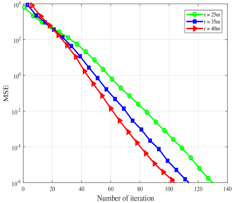
Figure 5: The MSE performance of LRM-CG for $k=2$ (2-dimensional location vectors).

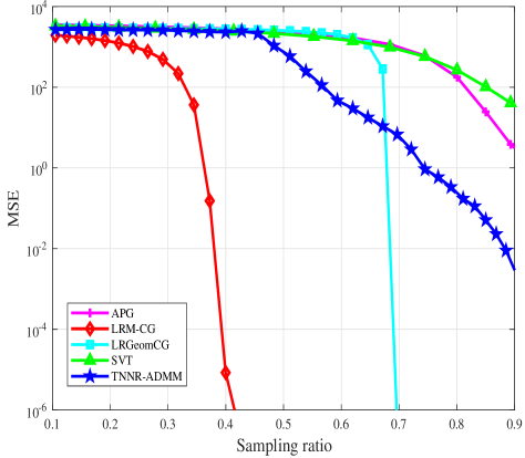
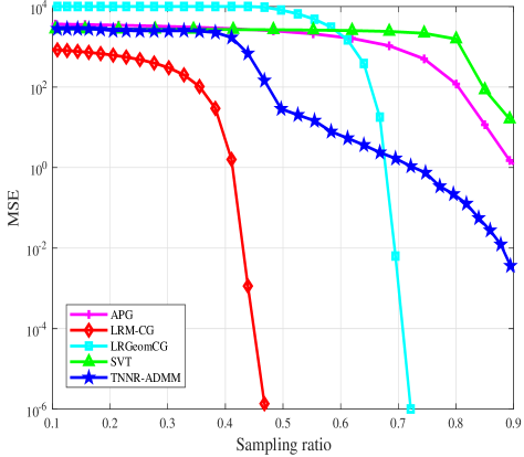
Figure 6: The MSE performance of the matrix completion algorithms for scenario without observation error for (a) 2-dimensional and (b) 3-dimensional location vectors.

V-A Convergence Efficiency

As performance measures, we use the mean square error (MSE) and the root mean square errors (RMSE), which are defined respectively as

$$MSE = \frac{1}{\sqrt{n^{2}-n}}\|\widehat{\mathbf{D}}-\mathbf{D}\|_{F},$$

$$RMSE = \sqrt{\frac{1}{n^{2}-n}\sum\limits_{i}\sum\limits_{j\neq i}(\widehat{d}_{ij}-d_{ij})^{2}}.$$

Note that the number of non-trivial entries of $\mathbf{D}$ is $n^{2}-n$ since the diagonal elements are zero (i.e., $d_{ii}=0$). Also, in order to compare the localization performance of the proposed algorithm, we use the mean square localization error (MSLE):

$$\mathcal{E} = \frac{1}{\text{Total unknown nodes}}\sum\limits_{\text{All unknown nodes i}}\|\widehat{\mathbf{x}}_{i}-\mathbf{x}_{i}\|_{2}.$$

In Fig. 5, we plot the log-scale MSE as a function of the number of iterations for the 2-dimensional sensor networks. Note that the results are obtained for the scenario where 200 sensor nodes are randomly distributed in $50\times 50$m² square area. We observe that the log-scale MSE decreases linearly with the number of iterations, meaning that the MSE decreases exponentially with the number of iterations. For example, if $r=35$m, it takes about 60, 80, and 100 iterations to achieve $10^{-1}$, $10^{-3}$, and $10^{-5}$, respectively. Also, as expected, required number of iterations to achieve the given performance level decreases with the radio communication range $r$.

V-B Performance Evaluation

In this subsection, we investigate the recovery performance of LRM-CG for scenarios with and without observation error. In Fig. 6, we plot the performance of the scenario without the observation error as a function of the sampling ratio, which is defined as the ratio of the number of observed pairwise distances to total number of pairwise distances. Here, the sampling ratio is controlled by the radio communication range $r$. We observe that LRM-CG outperforms conventional techniques by a large margin, achieving MSE $\leq 10^{-5}$ using 40% of measurements.

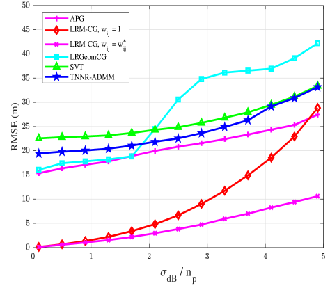
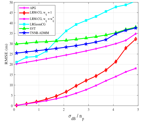
Figure 7: The RMSE performance of the algorithms in presence of observation errors for (a) 2-dimensional and (b) 3-dimensional location vectors.

In Fig. 7, we plot the performance of LRM-CG as a function of $\sigma_{dB}/n_{p}$. In this experiment, sensor nodes are randomly distributed in $50\times 50$m² square area ($k=2$) and $50\times 50\times 50$m³ cubic space ($k=3$). We set the radio communication range $r=30$m, resulting in 125 and 84 average connections per node for $k=2$ and $k=3$, respectively. While the performance of conventional matrix completion algorithms is poor (i.e., RMSE $\geq 5m$) in mid and high $\sigma_{dB}/n_{p}$ regime, the performance of LRM-CG is still good in small $\sigma_{dB}/n_{p}$ regime, achieving RMSE being less than 2.5m when $\sigma_{dB}/n_{p}\leq 1.5$.

We next investigate the localization performance of LRM-CG. We compare the performance of LRM-CG with the APG, LRGeomCG, SVT, TNNR-AMMD, MDS, and SDP-based algorithm [15]. In this experiment, 50 sensor nodes are randomly distributed in $50\times 50\times 50$m³ $(k=3)$ and 4 anchor nodes are used to reconstruct the global node locations. The stopping threshold $\epsilon$ of LRM-CG is set to $10^{-8}$. Since the reconstructed matrix of the conventional matrix completion algorithm including APG, LRGeomCG, SVT, and TNNR-AMMD, is not necessarily an Euclidean distance matrix, we use the MDS technique [10] as a post-processing to project the output matrix on the Euclidean distance matrix cone. In Fig. 8, we observe that conventional localization algorithms perform poor (MSLE $\geq 5m$) for mid and high $\sigma_{dB}/n_{p}$ regime, but the proposed LRM-CG algorithm performs well in low $\sigma_{dB}/n_{p}$ regime, achieving MSLE being less than 3m for $\sigma_{dB}/n_{p}\leq 1$.

We next examine the running time complexity of the algorithms under test as a function of the number of sensor nodes. In our simulations, we set the maximum iteration number to 200 and the stopping threshold $\epsilon$ of the matrix completion algorithms to $10^{-6}$. From Fig. 9, we observe that the running time of the SDP-based technique is fairly large since it should solve the primal and dual problems using SDPT3 solver [35, 36]. The running time of APG, LRGeomCG, MDS, and the proposed LRM-CG is more or less similar when $n\leq 200$. In Table I, we summarize the computational complexity of the algorithms under test in terms of flops. We observe that the computational complexity of LRM-CG is linearly proportional to the problem size $n$ and the number of the observed distances $|E|$, and thus competitive with the conventional approaches.

TABLE I: Computational complexity of the matrix completion algorithms in recovery of $n\times n$ rank-$k$ matrix.

Algorithms	Major computation	Total computational complexity per iteration
APG	Soft-thresholding SVD	$\mathcal{O}(\bar{k}n^{2})$a
LRM-CG	Truncated EVD	$\mathcal{O}(k^{2}n+k|E|)$
LRGeomCG	Truncated EVD	$\mathcal{O}(k^{2}n+k|E|)$
MDS	Truncated EVD	$\mathcal{O}(kn^{2})$
SDP	Convex operator	$\mathcal{O}(n^{3})$
SVT	Soft-thresholding SVD	$\mathcal{O}(\bar{k}n^{2})$
TNNR-ADMM	Soft-thresholding SVD	$\mathcal{O}(\bar{k}n^{2})$

• ^aNote that $\bar{k}$ is the number of singular values being larger than the threshold used in the soft-thresholding based SVD technique [22, 17, 33].

V-C Outlier Problem

We next investigate the performance of the proposed LRM-CG algorithm and its extended version (see Section IV) in the presence of outliers. When the outlier ratio $\theta$ is given, we randomly choose a set of the observed distances and replace this set by a set of random numbers. In this experiment, sensor nodes are randomly distributed in $50\times 50$m² square area. In our simulation, we consider the scenario in which the magnitude of outliers is comparable to the distance level. We could observe that the extended LRM-CG outperforms the original LRM-CG, achieving MSLE being less than 0.5m up to the 20% outlier ratio (see Fig. 10).

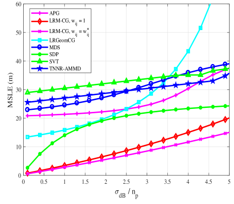
Figure 8: The RMSLE performance of the algorithms for 3-dimensional location vectors.

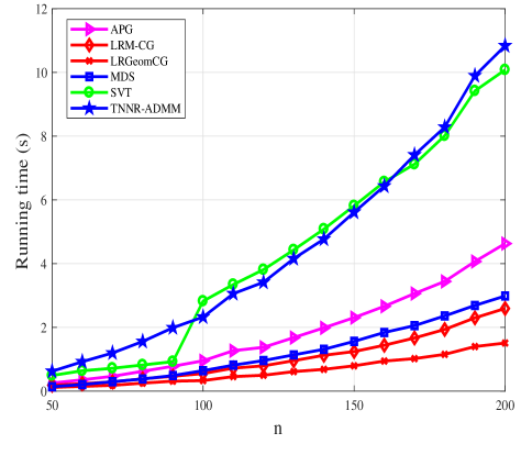
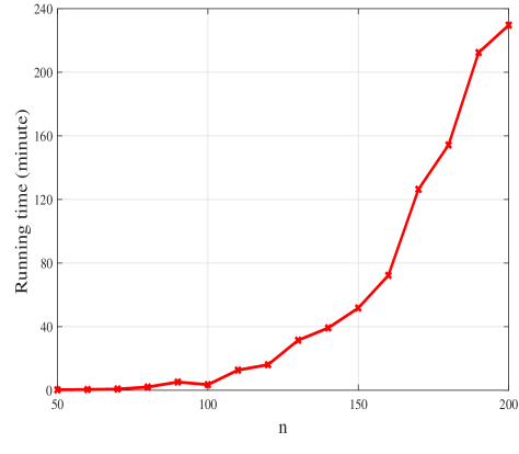
Figure 9: Running time as a function of the number of sensor nodes: (a) the conventional matrix completion algorithms and the proposed LRM-CG and (b) SDP-based algorithm. Since the running time of SDP-based algorithm is much higher than that of the other algorithms, we separate the results into two plots.

Figure 10: The MSLE performance of LRM-CG in the presence of outliers.

V-D Real Data

In this subsection, we examine the performance of the proposed LRM-CG algorithm using real measurements. In this simulation, we use the RSS-based measurement model in [34]. This network consists of 44 sensor nodes randomly distributed in the $14\times 14$m² square area and the transmit signal is generated via a wideband direct-sequence spread-spectrum (DSSS) operating at a center frequency of 2.4 GHz. For a given radio communication range $r$, we assume that $d_{ij}^{o}$ is known if $d_{ij}\leq r$ and unknown otherwise. We observe from Table II that the performance of the proposed LRM-CG is comparable to the SDP techniques in [15, 14] when $r=9.5m$.

TABLE II: Localization errors with real measurements.

$r$ (m)	Average connection per node	MSLE (m)
		LRM-CG	ELRM-CG	SDP with absolute cost function [15]	SDP with least square cost function [14]
5.5	14	5.4893	4.9860	4.5038	3.7241
7.5	22	5.2796	4.9170	3.1287	3.3394
9.5	30	2.9917	2.8620	2.9274	3.0526
11.5	37	2.2636	2.2023	2.6272	2.5151

VI Conclusion

In this paper, we have proposed an algorithm to recover the Euclidean distance matrix and the location map from partially observed distance information. In solving the Frobenius norm minimization problem with a rank constraint, we expressed the Euclidean distance matrix as a function of the low rank PSD matrix. By capitalizing on the Riemannian manifold structure for this set of matrices, we could solve the low-rank matrix completion problem using a modified nonlinear conjugate gradient algorithm. The proposed LRM-CG algorithm preserves the low rank structure of this reconstructed matrix. We have shown from the recovery condition analysis that the proposed LRM-CG algorithm converges to the original Euclidean distance matrix in the sampling space under the extended Wolfe’s conditions. We have also demonstrated from the numerical experiments that LRM-CG outperforms the conventional matrix completion techniques by a large margin, achieving MSE $\leq 10^{-5}$ using 40% of measurements. We also proposed an extended version of LRM-CG to control the outliers and demonstrated the effectiveness of the proposed scheme in the realistic environments with outliers. Given the importance of the location-aware applications and services in the IoT era, we believe that the proposed LRM-CG algorithm will be a useful tool for various localization scenarios. While our work focused primarily on the network localization scenario, extension to the distributed network scenarios would also be interesting direction worth pursuing.

Appendix A Proof of Theorem II.4

Proof.

Since $\nabla_{\mathbf{Y}}f(\mathbf{Y})$ is interpreted as a matrix whose inner product with an arbitrary matrix $\mathbf{H}$ becomes the Frechet differential $\text{D}f(\mathbf{Y})[\mathbf{H}]$ of $f$ at $\mathbf{Y}$, it is convenient to compute $\nabla_{\mathbf{Y}}f(\mathbf{Y})$ as a unique element of $\mathbb{R}^{n\times n}$ that satisfies

$$<\nabla_{\mathbf{Y}}f(\mathbf{Y}),\mathbf{H}>=\text{D}f(\mathbf{Y})[\mathbf{H}],$$ (39)

for all $\mathbf{H}$. We first compute $\text{D}f(\mathbf{Y})[\mathbf{H}]$ and then use (39) to obtain the expression of $\nabla_{\mathbf{Y}}f(\mathbf{Y})$. Let $h(\mathbf{R})=\frac{1}{2}\|\mathbf{R}\|_{F}^{2}$ and $k(\mathbf{Y})=\mathbf{W}\odot(\mathcal{P}_{E}\circ g)(\mathbf{Y})-\mathbf{W}\odot\mathcal{P}_{E}(\mathbf{D}_{o})$, then $f(\mathbf{Y})=h(k(\mathbf{Y}))=(h\circ k)(\mathbf{Y})$. Using matrix calculus, it is not hard to show that

$$\text{D}f(\mathbf{Y})[\mathbf{H}] = <2\text{eye}(\text{Sym}(\mathbf{W}\odot k(\mathbf{Y}))\mathbf{1})$$ (40)

$$-2\text{Sym}(\mathbf{W}\odot k(\mathbf{Y})),\mathbf{H}>$$

From (39) and (40), we have $\nabla_{\mathbf{Y}}f(\mathbf{Y})=2\text{eye}(\text{Sym}(\mathbf{W}\odot k(\mathbf{Y}))\mathbf{1})-2\text{Sym}(\mathbf{W}\odot k(\mathbf{Y}))$, which is the desired result.

∎

Appendix B Proof of Lemma III.4

Proof.

First, a lower bound of $\|\nabla_{\mathbf{Y}}f(\mathbf{Y}_{i})\|_{F}$ is given by

$$\|\nabla_{\mathbf{Y}}f(\mathbf{Y}_{i})\|_{F}^{2} \begin{subarray}{c}(a)\\ =\end{subarray} \|2\text{eye}(\mathbf{R}_{i}\mathbf{1})-2\mathbf{R}_{i}\|_{F}^{2}$$ (41)

$$\begin{subarray}{c}(b)\\ =\end{subarray} \|2\text{eye}(\mathbf{R}_{i}\mathbf{1})\|_{F}^{2}+\|2\mathbf{R}_{i}\|_{F}^{2}$$

$$\geq \|2\mathbf{R}_{i}\|_{F}^{2},$$

where (a) is from (14) and (b) is from the fact that diagonal entries of $\mathbf{R}_{j}$ are all zeros and $\text{eye}(\mathbf{R}_{j}\mathbf{1})$ is a diagonal matrix. That is, positions of nonzero elements in $\text{eye}(\mathbf{R}_{i}\mathbf{1})$ and $\mathbf{R}_{i}$ are disjoint. An upper bound is obtained as follows.

$$\|\nabla_{\mathbf{Y}}f(\mathbf{Y}_{i})\|_{F} \leq \|2\text{eye}(\mathbf{R}_{i}\mathbf{1})\|_{F}+\|2\mathbf{R}_{i}\|_{F}$$ (42)

$$\begin{subarray}{c}(a)\\ \leq\end{subarray} \|2\mathbf{R}_{i}\mathbf{1}\|_{2}+\|2\mathbf{R}_{i}\|_{F}$$

$$\begin{subarray}{c}(b)\\ \leq\end{subarray} 2\|\mathbf{R}_{i}\|_{F}\|\mathbf{1}\|_{2}+2\|\mathbf{R}_{i}\|_{F}$$

$$\leq (2\sqrt{n}+2)\|\mathbf{R}_{i}\|_{F},$$

where (a) is because $\|\text{eye}(\mathbf{b})\|_{F}=\|\mathbf{b}\|_{2}$ for any vector $\mathbf{b}$, and (b) is because $\|\mathbf{A}\mathbf{b}\|_{2}\leq\|\mathbf{A}\|_{F}\|\mathbf{b}\|_{2}$ for any matrix $\mathbf{A}$ and any vector $\mathbf{b}$. By combining (41) and (42), and noting that $\|\mathbf{R}_{i}\|_{F}=\|\mathcal{P}_{E}(\mathbf{D}_{i})-\mathcal{P}_{E}(\mathbf{D})\|_{F}$, we obtain the desired result. ∎

Appendix C Proof of Lemma III.7

Proof.

From A3, we have $\|\text{grad}f(\mathbf{Y}_{i})\|_{F}^{2}\geq\frac{1}{c^{2}}\|\nabla_{\mathbf{Y}}f(\mathbf{Y}_{i})\|_{F}^{2}$. Now, what remains is to show that $\|\nabla_{\mathbf{Y}}f(\mathbf{Y}_{i})\|_{F}^{2}\geq 8f(\mathbf{Y}_{i})$. Indeed, from Lemma II.4, we have

$$\frac{1}{4}\|\nabla_{\mathbf{Y}}f(\mathbf{Y}_{i})\|_{F}^{2} =\frac{1}{4}\|\text{eye}((\mathbf{R}+\mathbf{R}^{T})\mathbf{1})-2\mathbf{R}\|_{F}^{2}$$

$$=\|\text{eye}(\mathbf{R}\mathbf{1})\|_{F}^{2}+\|\mathbf{R}\|_{F}^{2}$$

$$-2<\text{eye}(\mathbf{R}\mathbf{1}),\mathbf{R}>$$

$$=\|\mathbf{R}\mathbf{1}\|_{2}^{2}+\|\mathbf{R}\|_{F}^{2}-2\sum\limits_{i}\left(\sum\limits_{j}r_{ij}\right)r_{ii}$$

$$=\|\mathbf{R}\mathbf{1}\|_{2}^{2}+\|\mathbf{R}\|_{F}^{2}$$

$$\geq\|\mathbf{R}\|_{F}^{2},$$ (43)

where $\mathbf{R}=\mathcal{P}_{E}(g(\mathbf{Y}_{i}))-\mathcal{P}_{E}(\mathbf{D})$ is symmetric with zero diagonal entries $r_{ii}=0$. Noting that $\|\mathbf{R}\|_{F}^{2}=2f(\mathbf{Y}_{i})$, we obtain the desired result. ∎

References

- [1] L. Nguyen, S. Kim, and B. Shim, “Localization in internet of things network: Matrix completion approach,” in Proc. Inform. Theory Applicat. Workshop, 2016.
- [2] L. Nguyen and B. Shim, “Localization of internet of things network via euclidean distance matrix completion,” in Proc. IEEE/CIC Int. Conf. Commun. China (ICCC)., 2016.
- [3] M. Delamo, S. Felici-Castell, J. J. Perez-Solano, and A. Foster, “Designing an open source maintenance-free environmental monitoring application for wireless sensor networks,” J. Syst. Softw., vol. 103, pp. 238–247, May 2015.
- [4] S. Lee, B. Koo, and S. Kim, “RAPS: reliable anchor pair selection for range-free localization in anisotropic networks,” IEEE Commun. Lett., vol. 18, pp. 1403–1406, 2014.
- [5] G. Hackmann, W. Guo, G. Yan, Z. Sun, C. Lu, and S. Dyke, “Cyber-physical codesign of distributed structural health monitoring with wireless sensor networks,” IEEE Trans. Parallel Distrib. Syst., vol. 25, pp. 63–72, Jan. 2014.
- [6] A. Pal, “Localization algorithms in wireless sensor networks: Current approaches and future challenges,” Netw. Protocols Algorithms, vol. 2, no. 1, pp. 45–74, 2010.
- [7] V. J. Hodge, S. O’Keefe, M. Weeks, and A. Moulds, “Wireless sensor networks for condition monitoring in the railway industry: A survey,” IEEE Trans. Intell. Transp. Syst., vol. 16, pp. 1088–1106, Jun. 2015.
- [8] P. Rawat, K. D. Singh, H. Chaouchi, and J. M. Bonnin, “Wireless sensor networks: a survey on recent developments and potential synergies,” J. Supercomput., vol. 68, no. 1, pp. 1–48, Apr. 2014.
- [9] J. Aspnes, T. Eren, D. Goldenberg, A. Morse, W. Whiteley, Y. Yang, B. Anderson, and P. Belhumeur, “A theory of network localization,” IEEE Trans. Mobile Comput., vol. 5, no. 12, pp. 1663–1678, Dec. 2006.
- [10] Y. Shang, W. Ruml, Y. Zhang, and M. Fromherz, “Localization from mere connectivity,” in Proc. ACM Symp. Mobile Ad Hoc Netw. Comput., Annapolis, Jun. 2003, pp. 201–212.
- [11] R. Parker and S. Valaee, “Vehicular node localization using received-signal-strength indicator,” IEEE Trans. Veh. Technol., vol. 56, pp. 3371–3380, Nov. 2007.
- [12] D. Dardari, C.-C. Chong, and M. Z. Win, “Threshold-based time-of-arrival estimators in uwb dense multipath channels,” IEEE Trans. Commun., vol. 56, pp. 1366–1378, Aug. 2008.
- [13] Y. Zhang and J. Zha, “Indoor localization using time difference of arrival and time-hopping impulse radio,” IEEE Int. Symp. Commun. Inform. Technol., pp. 964–967, Oct. 2005.
- [14] X. Guo, L. Chu, and X. Sun, “Accurate localization of multiple sources using semidefinite programming based on in complete range matrix,” IEEE Sensors J., vol. 16, no. 13, pp. 5319–5324, July 2016.
- [15] P. Biswas and Y. Ye, “Semidefinite programming for ad hoc wireless sensor network localization,” in Proc. 3rd Int. Symp. Inform. Process. Sensor Networks. ACM., pp. 46–54, 2004.
- [16] E. J. Candes and B. Recht, “Exact matrix completion via convex optimization,” Found. Comput. Math., vol. 6, pp. 717–772, 2009.
- [17] J.-F. Cai, E. J. Candes, and Z. Shen, “A singular value thresholding algorithm for matrix completion,” SIAM J. Optimiz., vol. 20, no. 4, pp. 1956–1982, 2010.
- [18] Z. Lin, M. Chen, and Y. Ma., “The augmented lagrange multiplier method for exact recovery of corrupted low-rank matrices,” arXiv:1009.5055, 2010.
- [19] B. Mishra, G. Meyer, and R. Sepulchre, “Low-rank optimization for distance matrix completion,” in Proc. 50th IEEE Conf. Decision Control Eur. Control Conf. (CDC-ECC), pp. 4455–4460, Dec. 2011.
- [20] P. Jain, P. Netrapalli, and S. Sanghavi, “Low-rank matrix completion using alternating minimization,” in Proc. 45th Annu. ACM Symp. Theory Comput., pp. 665–674, 2013.
- [21] J. Dattorro, Convex Optimization and Euclidean Distance Geometry, USA: Meboo Publishing, 2005.
- [22] Z. Lin, A. Ganesh, J. Wright, L. Wu, M. Chen, and Y. Ma, “Fast convex optimization algorithms for exact recovery of a corrupted low-rank matrix,” in Proc. Int. Workshop Comput. Adv. Multi-Sensor Adapt. Process., pp. 1–18, 2009.
- [23] P. A. Absil, R. Mahony, and R. Sepulchre, Optimization Algorithms on Matrix Manifolds, Princeton Univ. Press, 2008.
- [24] Z. Jianwu and Z. Lu, “Research on distance measurement based on rssi of zigbee,” ISECS Int. Colloq. Computing, Commun., Control, and Manage., pp. 210–212, 2009.
- [25] U. Helmke and J. B. Moore, Optimization and Dynamical Systems, London: Springer-Verlag, 1994.
- [26] B. Vandereycken, “Low-rank matrix completion by riemannian optimization,” SIAM J. Optimiz., vol. 23, no. 2, pp. 1214–1236, 2013.
- [27] P. A. Absil and J. Malick, “Projection-like retractions on matrix manifolds,” SIAM J. Optimiz., vol. 22, pp. 135–158, 2012.
- [28] Y. H. Dai, “Nonlinear conjugate gradient methods,” Wiley Encyclopedia of Operations Research and Manage. Sci., 2011.
- [29] W. W. Hager and H. Zhang, “A new conjugate gradient method with guaranteed descent and an efficient line search,” SIAM J. Optimiz., no. 1, pp. 170–192, 2005.
- [30] P. Wolfe, “Convergence conditions for ascent methods,” SIAM Rev., no. 2, pp. 226–235, 1969.
- [31] H. Sato and T. Iwai, “A new, globally convergent riemannian conjugate gradient method,” Optim. J. Math. Program. Oper. Res., no. 4, pp. 1011–1031, 2015.
- [32] Z. Yang, C. Wu, T. Chen, Y. Zhao, W. Gong, and Y. Liu, “Detecting outlier measurements based on graph rigidity for wireless sensor network localization,” IEEE Trans. Veh. Technol., vol. 62, no. 1, pp. 374–383, Jan. 2013.
- [33] Y. Hu, D. Zhang, J. Ye, X. Li, and X. He, “Fast and accurate matrix completion via truncated nuclear norm regularization,” IEEE Trans. Pattern Anal. Mach. Intell., no. 9, pp. 2117–2130, Sep. 2013.
- [34] J. A. Costa, N. Patwari, and I. A. O. Hero, “Distributed weighted-multidimensional scaling for node localization in sensor networks,” ACM Trans. Sensor Netw., vol. 2, no. 1, pp. 39–64, 2006.
- [35] K. C. Toh, M. J. Todd, and R. H. Tutuncu, “Sdpt3—a matlab software package for semidefinite programming,” Optimization Methods and Software, vol. 11, pp. 545–581, 1999.
- [36] R. H. Tutuncu, K. C. Toh, and M. J. Todd, “Solving semidefinite quadratic linear programs using sdpt3,” Math. Programming Ser. B, vol. 95, pp. 189–217, 2003.