Phase transitions in thick branes endorsed by entropic information

Abstract

The so-called configurational entropy (CE) framework has proved to be an efficient instrument to study nonlinear scalar field models featuring solutions with spatially-localized energy, since its proposal by Gleiser and Stamapoulos. Therefore, in this work, we apply this new physical quantity in order to investigate the properties of degenerate Bloch branes. We show that it is possible to construct a configurational entropy measure in functional space from the field configurations, where a complete set of exact solutions for the model studied displays both double and single-kink configurations. Our study shows a rich internal structure of the configurations, where we observe that the field configurations undergo a quick phase transition, which is endorsed by information entropy. Furthermore, the Bloch configurational entropy is employed to demonstrate a high organisational degree in the structure of the configurations of the system, stating that there is a best ordering for the solutions.

1 INTRODUCTION

In the last years, the study of phenomenological properties in braneworld models are increasing. We have recent works explaining anomalies in the meson $B$ decay [1] and in the neutrinos physics [2], performing bounds into corrections to Coulomb’s law [3, 4], into electrical conductivity [5], as also adjusting parameters to the experimental data of the nucleon-nucleus total cross-section of various chemical elements [6]. Applications to Myers-Perry’s black holes and results based on the observation of gravitational waves are others interesting issues about new insights in the braneworld framework.

In this context, a well-known model is the Bloch brane scenario, proposed by Bazeia and Gomes [9]. This thick brane model is generated by two interacting scalar fields that perform the thickness of the model that solves several issues in the fields localisation present in thin models [10, 11], as well as in the Randall-Sundrum models [12, 13]. Moreover, the structure of this scenario is based on domain walls, which have some interesting application in several branches of Physics as in high energy physics [14], cosmology [15, 16], quantum field theory [17] and propositions about the gravitational waves observation [18].

The authors of the works [20, 19, 21] have shown the existence of more general Bloch brane solutions in which a degeneracy parameter is responsible for the raising of two-kink solutions. That model is the so-called degenerate Bloch brane (DBB), where the energy of the field configuration in the superpotential is precisely the same with regarding all parameter associated with the domain wall [19]. So, we have the formation of a double brane structure with a splitting effect that is magnified by the approaching of the degeneracy parameter to a critical value.

This transition from single-kink solution to double-kink (or multi-kink) solutions have some physical implications. The multi-kinks appear in dispersive non-linear system, where single-kinks are no more stables [22]. The Ref. [23] shows the appearance of double-kink soliton in the sine-Gordon model under the perturbation of a space-dependent force. The experimental application of multi-kink concepts arises, among other, in the mobility hysteresis in a damped driven commensurable chain of atoms [24] and in arrays of Josephson junctions [25]. Specifically in the context of braneworlds, the presence of the massive resonant Kaluza-Klein modes is dependent upon transition parameter. A resonant KK mode is an extradimensional massive mode of a field with a finite lifetime, which can bring some interesting phenomenology to braneworlds branch [1, 4, 26, 27, 28]. The study of resonances for gravity and fermions in the symmetric and asymmetric cases of the usual Bloch branes was performed in Ref. [29]. However, more interesting results are present in the DBB scenarios [30, 21]. In this case the degeneracy constant tends to a critical value, a highly KK gravity mode coupled to the brane is observed [30], and also crucial issues in the localisation of massless fermions are clarified [21]. Moreover, the gauge field resonances are present only in the double-kink version of sine-Gordon models [4]. In short, the double-kink models bring more stability to the models and richer physical applications.

On the other hand, the reference [31] reintroduces the concept of informational entropy, based on Shannon’s information entropy [32]. The so-called Configurational Entropy (CE) was constructed and applied to several nonlinear scalar field models featuring solutions with spatially-localised energy. As presented in Ref. [31], the CE can solve energies of degenerate configurations. The approach presented in [31] have been used to study the non-equilibrium dynamics of spontaneous symmetry breaking [33], to obtain the stability bound for compact objects like Q-balls [34], to investigate the emergence of localized objects during inflationary preheating [35], and moreover to distinguish configurations with energy-degenerate spatial profiles [36]. The CE bounds the stability of various self-gravitating astrophysical objects [37] and states in Lorentz Violating (LV) scenarios [38] and also provides information about the stability of the glueball states in a dynamical holographic AdS/QCD model [39]. In the topic of braneworlds, the CE was heretofore applied to sine-Gordon models [40], to models with $f(R)$ [41], to $f(R,T)$ [42] theories of gravity, and to the Weyl brane [43], as well as to the topological abelian string-vortex in six dimensions [44].

Guided by the previous results involving degenerate two-field thick brane solutions, we propose in this work to investigate the Bloch brane solutions and degenerate versions by means of the CE information.

2 Bloch brane overview

A very interesting class of configuration in theories involving extra dimensions is that one where the scalar field give rise a domain wall, which is baptised in the literature as thick brane. It was shown that some kinds of two interacting scalar field potentials can be used in order to describe the splitting of thick branes due to a first-order phase transition in a warped geometry. As a consequence, we can find remarkable and distinctive critical phenomena in warped spacetimes, which can open a new window to study cosmological scenarios. Other efficient alternative to find answers for the cosmological issues come from the work by Bazeia and Campos [9], where it was studied a system described by two real scalar fields coupled with gravity in $\left(4+1\right)$ dimensions in warped spacetime involving one extra dimension. In that work, it was found a rich class of brane configuration, which was called Bloch brane. The most important feature of the Bloch brane solutions is its stability regarding the classical linear fluctuations of the scalar fields.

2.1 Bloch brane

The simplest Bloch brane setup is built with the coupling of two fields to gravity, as we describe below. The scalar fields depend only on the extra dimension $y$. The usual action in five-dimensional ($5D$) gravity can be represented by

$$S=\int{d^{4}xdy}\sqrt{\lvert g\lvert}\left[-\frac{R}{4}+\frac{1}{2}\left(\partial_{\mu}\phi\partial^{\mu}\phi+\partial_{\mu}\chi\partial^{\mu}\chi\right)-V\left(\phi,\chi\right)\right],$$ (1)

where $g=det(g_{\mu\nu})$ and $R$ is the curvature scalar for the metric $ds^{2}=\operatorname{e}^{2A}\eta_{\mu\nu}dx^{\mu}dx^{\nu}-dy^{2}$. From Eq. (1), we can obtain the following equation of motion and the corresponding modified Einstein equations

$$\phi^{\prime\prime}+4A^{\prime}\phi^{\prime}=\frac{\partial V}{\partial\phi},\quad\chi^{\prime\prime}+4A^{\prime}\chi^{\prime}=\frac{\partial V}{\partial\chi}$$ (2)

$$A^{\prime\prime}=-\frac{2}{3}\left(\phi^{\prime 2}+\chi^{\prime 2}\right)$$ (3)

$$A^{\prime 2}=\frac{1}{6}\left(\phi^{\prime 2}+\chi^{\prime 2}\right)-\frac{1}{3}V(\phi,\chi).$$ (4)

where prime stands for derivative with respect to $y$.

In order to obtain first order equations from the equations of motion, let us apply the so-called superpotential method [45, 46, 47, 48, 49, 50, 51]

$$V(\phi,\chi)=\frac{1}{8}\left[\left(\frac{\partial W}{\partial\phi}\right)^{2}+\left(\frac{\partial W}{\partial\chi}\right)^{2}\right]-\frac{1}{3}W^{2}(\phi,\chi).$$ (5)

where $W(\phi,\chi)$ is the superpotential, which from Ref. [45] is defined by

$$W(\phi,\chi)=2\phi-\frac{2}{3}\phi^{3}-2r\phi\chi^{2}\ ,\$$ (6)

where $r$ is a real thickness parameter that can vary in the interval $r\in(0,1/2)$.

We want to stress, however, that this particular superpotential has a fertile structure being very useful in a large number of physical applications. For instance, studies include topological defects, localisation of fermions on critical branes, supersymmetric theories, travelling solitons in Lorentz and CPT breaking systems, bags, junctions, and networks of BPS and non-BPS defects [45, 9, 20, 19, 21].

With the potential introduced in Eq.(5), we obtain the resulting first-order equations $\phi^{\prime}=\frac{1}{2}\frac{\partial W}{\partial\phi}$, $\chi^{\prime}=\frac{1}{2}\frac{\partial W}{\partial\chi}$ and $A^{\prime}=-\frac{1}{3}W$, from which we find the solutions that describe our brane model. The solutions to the fields are

$$\phi(y)=\tanh(2ry),\ \chi(y)=\pm\left(\sqrt{\frac{1}{r}-2}\right)\operatorname{sech}(2ry)\ .$$ (7)

The upper limit $r\rightarrow 1/2$ changes the Bloch brane profile, where two-field solution turns into one-field solution [9]. However, for the usual Bloch brane the two-kink profile is never achieved by variations in $r$. The warp factor $e^{2A(y)}$ is obtained by the solution of $A^{\prime}=-W/3$ in the form

$$A(y)=\frac{1}{9r}\left[(1-3r)\tanh^{2}(2ry)-2\ln\cosh(2ry)\right].$$ (8)

For this model, the energy density is written as [9]

$$\varepsilon(y)=\operatorname{e}^{2A(y)}\left[\frac{1}{2}\phi^{\prime 2}+\frac{1}{2}\chi^{\prime 2}+V(\phi,\chi)\right].$$ (9)

We plot $\varepsilon(y)$ in Fig. (1), that show us the appearance of two peaks on the energy density for the interval $0>r>0.17$. In Ref. [9] the authors have noticed the existence of a brane internal structure that is suppressed by the presence of gravity. The raising of such structure is related with a specific value of $r$. This issue will be addressed in the next section by CE concepts.

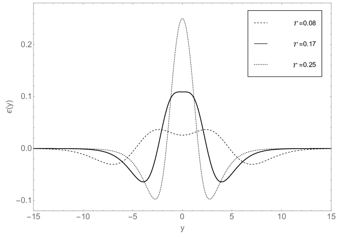
Figure 1: $\varepsilon(y)$ for Bloch brane.

2.2 Degenerate I Bloch Brane

Among other types of nonlinear field configurations coupled to gravity in (4 + 1) dimensions in warped space-time with one extra dimension. That is a specially important class of Bloch branes, which was coined degenerate Bloch brane (DBB) [19, 21], due to degenerate energy in the superpotencial parameters. These new class of configurations, on the contrary of the usual Bloch branes, enable a control over the brane thickness without needing to change the potential parameter, but by means of a domain wall degeneracy parameter.

In such models, the scalar field manifests a transition from kink to double kink solution when a degeneracy parameter reaches a critical value with the following potential:

$$V(\phi,\chi)=\frac{1}{2}\left[\left(\frac{\partial W}{\partial\phi}\right)^{2}+\left(\frac{\partial W}{\partial\chi}\right)^{2}\right]-\frac{4}{3}W^{2}(\phi,\chi),$$ (10)

and the new superpotential

$$W(\phi,\chi)=\phi\left[\lambda\left(\frac{\phi^{2}}{3}-a^{2}\right)+\mu\chi^{2}\right],$$ (11)

where $\lambda$, $a$ and $\mu$ are real parameters that deform this superpotential.

So, it has been found in Ref. [20] that there are two particular cases where the first-order differential equations can be solved analytically. The first set of solutions is given by [19]

$$\chi^{(1)}(y) = \frac{2a^{2}}{\left(\sqrt{c_{0}^{2}-4a^{2}}\right)\cosh(2\mu ay)-c_{0}},\quad$$ (12)

$$\phi^{(1)}(y) = \frac{a\left(\sqrt{c_{0}^{2}-4a^{2}}\right)\sinh(2\mu ay)}{\left(\sqrt{c_{0}^{2}-4a^{2}}\right)\cosh(2\mu ay)-c_{0}},$$ (13)

where $c_{0}$ is the degeneracy parameter that also regulates the brane thickness (the larger is $c_{0}$, the thinner is the brane) and it was considered as $c_{0}<-2a$ and $\lambda=\mu$. Moreover, in this case, the corresponding warp factor is written in the form

$$e^{A(y)}=N\left[\frac{2a^{2}}{\left(\sqrt{c_{0}^{2}-4a^{2}}\right)\cosh(2\mu ay)-c_{0}}\right]^{\frac{4}{9}a^{2}}\times$$

$$\times\exp\left\{\frac{2a^{2}\left[c_{0}^{2}\pm 4a^{2}-c_{0}\left(\sqrt{c_{0}^{2}-4a^{2}}\right)\cosh(2a\mu y)\right]}{9\left[\left(\sqrt{c_{0}^{2}-4a^{2}}\right)\cosh(2\mu ay)-c_{0}\right]^{2}}\right\}.$$ (14)

An interesting feature of these solutions is that, for some values of $c_{0}$ close to the critical value, namely $c_{0}^{crit}=-2a$, the scalar field $\phi^{(1)}(y)$ exhibits a double kink profile that reflects a formation of a double wall structure, extended along the extra dimension. On the other hand, the scalar field $\chi^{(1)}(y)$, close to the critical value $c_{0}^{crit}$, exhibits a flat top. In addition, we can observe in the warp factor the emergence of a controllable flat region, where one could think in a Minkowski-type metric region sandwiched between the two branes.

As we are interested in analysing the information-entropic measure of these configurations, it is interesting to show the energy density profile. Therefore with the results above we are able to construct the energy density (9), which is displayed in Fig. (2). From that figure, we can also note the appearance of two peaks when the degeneracy parameter is close to the critical value, signalising a richer structure for energy density.

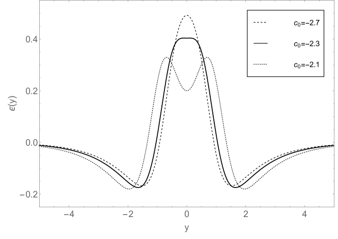
Figure 2: $\varepsilon(y)$ for DBB I with $a=\mu=1$.

2.3 Degenerate II Bloch Brane

Following Ref. [21], with the same potential (10) and the superpotential function (11), there is another class of degenerate Bloch brane solution, which we named DBB II. In this case, assuming $c_{0}<1/(16a^{2})$ and $\lambda=4\mu$, we find the following analytical solutions [21]

$$\chi^{(2)}(y)=-\frac{2a}{\sqrt{\left(\sqrt{1-16c_{0}a^{2}}\right)\cosh(4\mu ay)+1}},$$ (15)

$$\quad\phi^{(2)}(y)=\frac{a\left(\sqrt{1-16c_{0}a^{2}}\right)\sinh(4\mu ay)}{\left(\sqrt{1-16c_{0}a^{2}}\right)\cosh(4\mu ay)+1}.$$ (16)

Furthermore, the corresponding warp factor is given by

$$e^{2A(y)}=N\left[-\frac{2a}{\sqrt{\left(\sqrt{1-16c_{0}a^{2}}\right)\cosh(4\mu ay)+1}}\right]^{\frac{16a^{2}}{9}}\times$$

$$\times\exp\left\{-\frac{4a^{2}\left[1+8c_{0}a^{2}+\left(\sqrt{1-16c_{0}a^{2}}\right)\cosh(4a\mu y)\right]}{9\left[\left(1+\sqrt{1-16c_{0}a^{2}}\right)\cosh(4\mu ay)\right]^{2}}\right\}.$$ (17)

The solution presented in (17) is also known as critical Bloch brane due the appearance of a more pronounced flat region when the degeneracy parameter tends to its upper limit $c_{0}\to\left(1/16a^{2}\right)$. After all, we note that the DBB I and DBB II are very similar models, as we can see by comparing the warp factors in the equations (14) and (17).

Finally, the resulting energy density is plotted in Fig. (3).

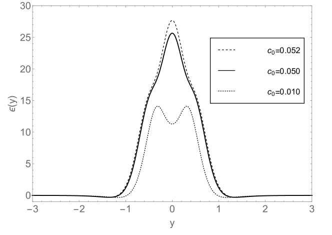
Figure 3: $\varepsilon(y)$ for DBB II with $a=\mu=1$.

The behaviour of the energy density of the DBB II solution is different from the two previous cases, since its energies are more localised and the peaks are more prominent. However, the DBB II model maintains the splitting of the maxima. In next section, we will verify by CE concepts, that these changes in the DBB II occur because the region where CE tends to the minimum is more narrow that in the DBB I and in the usual Bloch Brane cases.

3 Configurational Entropy in Bloch brane scenario

The so-called configurational entropy (CE) [31] is correlated to the energy of a localised field configuration, where low energy systems are linked with small entropic measures [31].

The CE can be expressed by the following Fourier transform of the energy density [40, 41, 31]

$$\mathcal{F}(\omega)=\frac{1}{\sqrt{2\pi}}\int_{-\infty}^{\infty}{\varepsilon(y)\operatorname{e}^{i\omega y}dy}.$$ (18)

The model where we apply the CE contains structures with spatially localised, square-integrable, bounded energy density functions $\varepsilon(y)$. Hence, we can define the so-called modal fraction that reads [31, 34, 33, 36]

$$f(\omega)=\frac{{\lvert\mathcal{F}(\omega)\lvert^{2}}}{{\int_{-\infty}^{\infty}{d\omega\lvert\mathcal{F}(\omega)\lvert^{2}}}\,}.$$ (19)

Subsequently, we can work with the normalized modal fraction, defined as the ratio of the normalised Fourier transformed function and its maximum value $\tilde{f}(\omega)={f(\omega)}/{f_{max}}.$ So, localised and continuous function $\tilde{f}(\omega)$ yields the following definition for the CE

$$S(\tilde{f})=-\int_{-\infty}^{\infty}{d\omega}\tilde{f}(\omega)\mbox{ln}\left[\tilde{f}(\omega)\right].$$ (20)

From the point of view of CE approach, it has been shown that is possible to obtain important bounds in theories where unknown parameters are presented. Here, it should be noted that the strategy of using $c_{0}$ to map a different range of parameters for the energy density and the CE has been used successfully several times before. It is worth highlighting that the CE method was already employed for the flat case of degenerate kinks in two-field models [36]. In the present paper, we verify the influence of the gravity in these degenerate models and its implications on the fields localisation and the changes in the critical points. The main motivation in our study is to show that there is a bound regarding the internal structure of DBB, where the warped geometry leads to the emergence of a controllable flat region, which is described by a Minkowski space-time. Through this analysis, we expect to understand the phase transition phenomena in Bloch branes scenarios, providing tools for a better understanding of new brane cosmological models. Furthermore, we can point out the most probable parameter that allows us to have normalisable fermion zero-mode localised on the brane. In addition we have the value for the highly KK gravity modes coupled in these DBB models. Our methodology consists in quantify the CE in terms of the degeneracy parameter $c_{0}$. On this way, we can merge the entropy information with details of the structure of the defects like thickness and curvature.

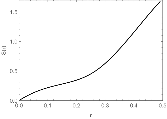
Figure 4: CE for usual Bloch brane solution.

3.1 CE in the usual Bloch Brane

Now, we review the CE approach to the usual Bloch brane. Firstly we analyse the basic two-field setup from Eqs. (7). Due to the complexity of the solutions, we evaluate numerically the $S(\tilde{f})$ and show the result in Fig. (4). The graphic shows us that there is no minimum in the CE to this case and $S(\tilde{f})$ is reduced as the thickness of the brane is increased ($r$ goes to zero). This result tells us that the region where we have the opening of the internal structure, namely, $0<r<0.17$, corresponds to the region of lower CE. Therefore, in the range of lowest CE, the coupling to gravity does not destroy the presence of internal structure for the Bloch brane. From information-entropic measure point of view, that range matches the values of lower energy of the system, and thus explaining the stability of the configurations. This is an important result from CE background, since that the problem concerning the stability of internal structure had not yet been sufficiently answered in the literature.

The lack of a minimum CE for $r\neq 0$ is related to the absence of a phase transition in the scalar field solutions. In fact, the solution to $\phi(y)$ in this case do not presents the transition kink to double-kink profile. In addition, the CE shows that the most prominent Bloch configurations are those where the interaction between the fields is weak. In this case, we can argue that the CE selects usual Bloch brane models that in a good approximation has its form dominated by the standard $\phi^{4}$ model.

3.2 CE in the degenerate I Bloch brane

We now turn our attention to the DBB I solution, that is expressed by the solutions in Eqs. (12) and (14). After numerical calculations, the CE for this case is presented in Fig. (5). Our fundamental goal is to show that the CE can be used to distinguish between such configurations. Moreover, as a Bloch brane is a thick brane that evolutes to a thicker one, which is called DBB, we are interested in describing the mechanism that can adequately facilitate the description of first order phase transitions. As a matter of fact, these transitions can provide a better understanding of the complex issues regarding brane splitting in warped geometries. In this case, we will see that the CE can be used as a key element for this description.

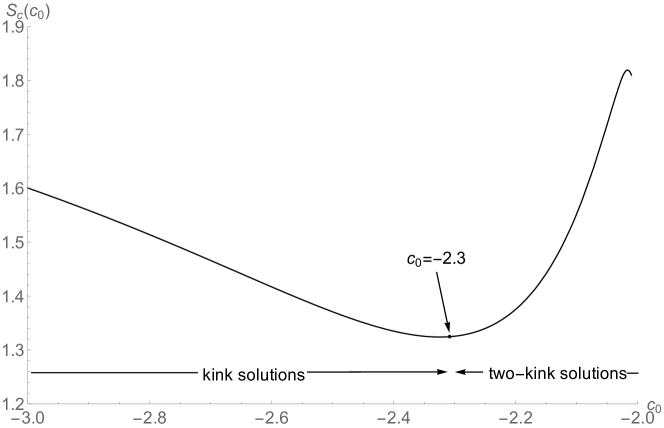
Figure 5: CE for DBB I solution with $a=\mu=1$.

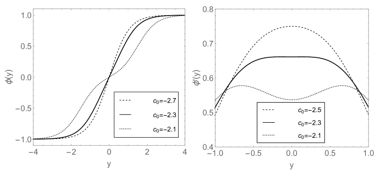
Figure 6: Scalar field solution for DBB I case (left) and its first derivative (right) for $a=\mu=1$.

From the Fig. (5), we can note that there is a minimum in the CE at $c_{0}=-2.3$. This point corresponds the phase transition for the scalar field solution. At this point, we have the raising of two-kink profile. In order to better identify the raising of the two-kink solutions, we have plotted the first derivative of the scalar field in Figure (6). In one-kink solution, the first derivative must assume a constant value near the origin. However, when we have the two-kink solution, the $\phi^{\prime}(0)$ must be a local minimum. We note the appearance of a minimum in $\phi^{\prime}(0)$ at the critical point ($c_{0}=-2.3$). Therefore, the raising of two-kink profile occurs at the degeneracy parameter $c_{0}$ corresponding to the minimum of the CE.

There is also a correspondence between the entropic information and the matter-energy density along the extra dimension. For the region where $c_{0}<-2.3$, the $\varepsilon(y)$ degenerate solutions have a single peak around $y=0$. Our results also show that for $-2.3<c_{0}<-2.0$ (see fig.( 2)) the energy density acquires two peaks. The minimum of the CE at $c_{0}=-2.3$ is related to the appearance of a behavior named brane internal structure, as reported in ref. [9].

3.3 CE in the degenerate II Bloch brane

The CE for the second class of degenerate solution is showed in Figure (7). We also have a minimum entropy point defining the frontier between the regions with kink and two-kink solutions. Since that the Fig. (3) shows a more narrow and localised energy density, we verify by its CE in Fig. (7) that the interval where we have two-kink solutions should be very small. The minimum entropy $c_{0}=0.05$ corresponds to the beginning of the formation of two-kink solutions. This also can be verified by the scalar field and its derivative in terms of $c_{0}$ near the phase transition, as plotted in Figure (8). For the kink structure, the $\phi^{\prime}(0)$ must have a maximum. However, in the interval $0.05<c_{0}<0.06$ we have a local minimum to $\phi^{\prime}(0)$ indicating the emergence of two-kink profile.

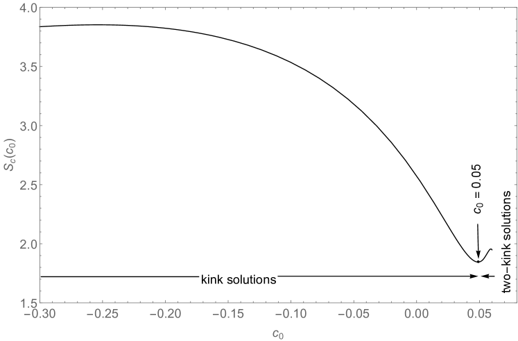
Figure 7: CE for DBB II solution with $a=\mu=1$

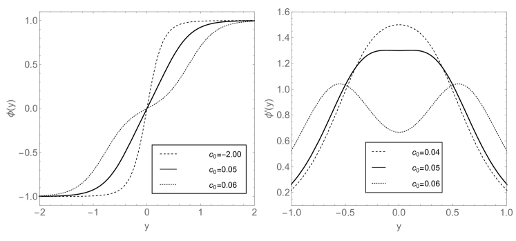
Figure 8: Scalar field solution for DBB II case (left) and its first derivative (right) for $a=\mu=1$.

4 Discussion and conclusions

We investigated the properties of a $5D$ braneworld generated by two scalar fields coupled to gravity from the viewpoint of the Configurational Entropy (CE) measure. The Bloch brane model is especially interesting in this scenario because it has a degenerate spatially-localised energy. The connection with the entropic information and the model is stated via the matter-energy density along the extra dimension. From the Fourier transform of the energy density, we construct a relation between each degenerate energy density and its resulting CE.

The first new result is revealed when we consider the basic two-field thick brane setup. The increasing of the brane thickness and the raising of the internal structure occurs at the lowest entropy values. There is no phase transition of the scalar field solutions of the basic Bloch brane and this is expressed with the absence of local or global minima in the CE, as showed in Fig. (4).

For the Degenerate I Bloch Brane (DBB I) solution, the information entropy reveals us special details concerning the brane formation. The link between the CE and the degenerate energy density solutions is presented in Fig. (5). The minimum CE for this case is $1.32$ and corresponds to the degenerate parameter $c_{0}=-2.3$. This is the turning point of the DBB I solution. Regarding the energy density, the lowest CE value corresponds to the raising of the internal structure, which can be observed in Fig. (2). We also observed that at minimum $S(\tilde{f})$ there is a phase transition where the kink solution to $\phi(y)$ converges into a two-kink one.

The DBB II case also presents a splitting effect in the energy density, however, it happens to a distinct value of the CE at the scalar field phase transition. The region where the CE tends to the minimum value is narrow, which reflects the narrow density energy distributions for this second model and, as expected, the interval where the two-kink solutions exists is very small if compared with DBB I scenario.

One very important consequence of our analysis is that the flat region in the warp factor undergo a kind of phase transition in a certain value of the degeneracy parameter, which is designated by the CE. Thus, such approach enables to predict which is the approximate value of the degeneracy parameter, and if the confining mechanism for the bulk particles will occur in that internal region. For instance, in scenarios where there is the localisation of fermions [21] on the degenerate Bloch branes, the CE provides the correct values of $c_{0}$ for the localisation of fermionic zero modes inside the branes. Here, it is important to remark that the values of $c_{0}$ are in accordance with that one found in ref. [21]. Moreover, for the DBB II model, the double-kink region enables the existence of a strong resonant graviton coupled to brane with a larger lifetime [30].

The investigation in braneworld models using the CE approach can reveal interesting features of these kind of models. We will continue addressing this issue in future works.

5 Acknowledgments

This work was partially supported by the Brazilian agencies Coordenação de Aperfeiçoamento de Pessoal de Nível Superior (CAPES) (grant no. 99999.
006822/2014-02), Conselho Nacional de Desenvolvimento Científico e Tecnológico (CNPq) (grant numbers 305766/2012-0 and 305678/2015-9) and São Paulo Research Foundation (FAPESP) (grant 2016/03276-5). The authors are very thankful for the referee suggestions.

References

References

- [1] E. Megias, G. Panico, O. Pujolas and M. Quiros, JHEP 1609, 118 (2016)
- [2] P. Chen, G. J. Ding, A. D. Rojas, C. A. Vaquera-Araujo and J. W. F. Valle, JHEP 1601, 007 (2016).
- [3] R. Cartas-Fuentevilla, A. Escalante, G. German, A. Herrera-Aguilar and R. R. Mora-Luna, JCAP 1605, no. 05, 026 (2016).
- [4] W. T. Cruz, R. V. Maluf, D. M. Dantas and C. A. S. Almeida, Annals Phys. 375, 49 (2016).
- [5] T. N. Ikeda, A. Lucas and Y. Nakai, JHEP 1604, 007 (2016).
- [6] R. Arceo, O. Pedraza, L. A. Lopez, L. Valencia-Palomo, E. Gonzalez-Espinosa, G. Leon-Soto and S. Kurtz, Int. J. Mod. Phys. E 25, no. 10, 1650084 (2016).
- [7] M. Stein, JHEP 1609, 067 (2016).
- [8] H. Yu, B. M. Gu, F. P. Huang, Y. Q. Wang, X. H. Meng and Y. X. Liu, JCAP 1702, no. 02, 039 (2017)
- [9] D. Bazeia and A. R. Gomes, J. High Energy Phys. 0405 (2004) 012.
- [10] V. Dzhunushaliev, V. Folomeev, and M. Minamitsuji, Rept. Prog. Phys. 73, 066901 (2010).
- [11] B. Bajc, G. Gabadadze, Phys. Lett. B 474, 282 (2000).
- [12] L. Randall and R. Sundrum, Phys. Rev. Lett. 83, 3370 (1999).
- [13] L. Randall and R. Sundrum, Phys. Rev. Lett. 83, 4690 (1999).
- [14] A. Vilenkin and E.P.S. Shellard, Cosmic strings and other topological defects, Cambridge University Press, Cambridge 1994.
- [15] S. E. Larsson, S. Sarkar and P. L. White, Phys. Rev. D 55, 5129 (1997)
- [16] K. Skenderis and P. K. Townsend, Phys. Rev. D 74, 125008 (2006)
- [17] H. J. Boonstra, K. Skenderis and P. K. Townsend, JHEP 9901, 003 (1999)
- [18] T. Krajewski, Z. Lalak, M. Lewicki and P. Olszewski, JCAP 1612, no. 12, 036 (2016)
- [19] A. de Souza Dutra, A. C. A. de Faria, Jr. and M. Hott, Phys. Rev. D 78, 043526 (2008).
- [20] A. de Souza Dutra, Phys. Lett. B 626, 249 (2005).
- [21] R. A. C. Correa, A. de Souza Dutra and M.B.Hott, Class. Quant. Grav. 28, 155012 (2011).
- [22] G. P. de Brito, R. A. C. Correa and A. de Souza Dutra, Phys. Rev. D 89, no. 6, 065039 (2014).
- [23] M. A. Garcia-Nustes and J. A. Gonzalez, Phys. Rev. E 86, 066602 (2012).
- [24] O.M. Braun, T. Dauxois, M.V. Paliy, and M. Peyrard. Phys. Rev. Lett. 78, 1295 (1997).
- [25] A.V. Ustinov, B.A. Malomed, and S. Sakai. Phys. Rev. B 57, 11691 (1998).
- [26] H. Davoudiasl, J. L. Hewett and T. G. Rizzo, Phys. Rev. Lett. 84, 2080 (2000).
- [27] S. Kumar Rai and S. Raychaudhuri, JHEP 0310, 020 (2003).
- [28] J. C. B. Araujo, D. F. S. Veras, D. M. Dantas and C. A. S. Almeida, arXiv:1610.08124 [hep-th].
- [29] Q. Y. Xie, J. Yang and L. Zhao, Phys. Rev. D 88, 105014 (2013).
- [30] W. T. Cruz, L. J. S. Sousa, R. V. Maluf and C. A. S. Almeida, Phys. Lett. B 730 (2014) 314.
- [31] M. Gleiser and N. Stamatopoulos, Phys. Lett. B 713, 304 (2012).
- [32] C. E. Shannon, The Bell System Technical J. 27, 379 (1948).
- [33] M. Gleiser and N. Stamatopoulos, Phys. Rev. D 86, 045004 (2012).
- [34] M. Gleiser, D. Sowinski, Phys. Lett. B 727, 272 (2013).
- [35] M. Gleiser, N. Graham, Phys. Rev. D 89, 083502 (2014).
- [36] R. A. C. Correa, A. de Souza Dutra, and M. Gleiser, Phys. Lett. B 737, 388 (2014).
- [37] M. Gleiser and N. Jiang, Phys. Rev. D 92, 044046 (2015).
- [38] R. A. C. Correa, R. da Rocha, and A. de Souza Dutra, Ann. Phys. 359, 198 (2015).
- [39] A. E. Bernardini, N. R. F. Braga and R. da Rocha, Phys. Lett. B 765, 81 (2017)
- [40] R. A. C. Correa and R. da Rocha, Eur. Phys. J. C 75, 522 (2015).
- [41] R. A. C. Correa, P. H. R. S. Moraes, A. de Souza Dutra, and R. da Rocha, Phys. Rev. D 92, 126005 (2015).
- [42] R. A. C. Correa and P. H. R. S. Moraes, Configurational entropy in brane models, [arXiv:1509.00732].
- [43] R. A. C. Correa, D. M. Dantas, C. A. S. Almeida and P. H. R. S. Moraes, Refinements of the Weyl pure geometrical thick branes from information-entropic measure, arXiv:1607.01710 [hep-th].
- [44] R. A. C. Correa, D. M. Dantas, C. A. S. Almeida and R. da Rocha, Phys. Lett. B 755, 358 (2016)
- [45] D. Bazeia, M.J. dos Santos and R.F. Ribeiro, Phys. Lett. A 208 84 (1995).
- [46] D. Bazeia, H. Boschi-Filho, and F.A. Brito, J. High Energy Phys. 9904 (1999) 028.
- [47] D. Bazeia and F.A. Brito, Phys. Rev. Lett. 84, 1094 (2000).
- [48] D. Bazeia, J.R. Nascimento, R.F. Ribeiro and D. Toledo, J. Phys. A 30, 8157 (1997).
- [49] M.A. Shifman and M.B. Voloshin, Phys. Rev. D 57, 2590 (1998).
- [50] A. Alonso Izquierdo, M.A. Gonzalez Lion and J. Mateos Guilarte, Phys. Rev. D 65, 085012 (2002).
- [51] D. Bazeia, E. E. M. Lima and L. Losano, Eur. Phys. J. C 77, no. 2, 127 (2017).