Cavity mediated effective interaction between phonon and magnon

Abstract

Optomagnonics and optomechanics have various applications ranging from tunable light sources to optical manipulation for quantum information science. Here, we propose a hybrid system with the interaction between phonon and magnon which could be tuned by the electromagnetic field based on the radiation pressure and magneto-optical effect. The self energy of the magnon and phonon induced by the electromagnetic field and the influence of the thermal noise are studied. Moreover, the topological features of the hybrid system is illustrated with resort to the dynamical encircling with the exceptional points, and the chiral characteristics under these encirclements are found.

I Introduction

Optomechanics Bowen-Milburn ; RevModPhys.86.1391 ; Aspelmeyer ; Kippenberg:07 ; peng2014and ; anetsberger2009near ; Kippenberg1172 ; hill2012coherent ; PhysRevLett.110.153606 ; PhysRevLett.98.150802 ; thompson2008strong and optomagnonics PhysRevLett.113.156401 ; PhysRevB.94.060405 ; PhysRevLett.117.123605 ; PhysRevA.92.063845 ; PhysRevB.93.144420 ; PhysRevLett.116.223601 ; PhysRevLett.117.133602 ; PhysRevA.94.033821 ; klos2014photonic ; chumak2015magnon ; Tabuchi405 ; PhysRevLett.111.127003 are both hybrid optical interaction which could be achieved on the microresonator system. Efficient and low-noise optomechanics has many applications in classical and quantum photonics, such as squeezed light generation brooks2012non ; safavi2013squeezed ; PhysRevX.3.031012 ; PhysRevA.83.033820 ; PhysRevA.82.021806 , mass and force sensing PhysRevLett.97.133601 ; PhysRevLett.105.123601 ; teufel2009nanomechanical ; PhysRevLett.113.020405 , optical manipulation PhysRevLett.112.013602 ; Weis1520 ; monifi2016optomechanically ; safavi2011electromagnetically ; jing2015optomechanically , and so on. Moreover, optomechanics also provides us a platform to study the basic tasks of quantum information processing PhysRevLett.109.013603 ; Ying-Dan ; PhysRevLett.111.083601 ; PhysRevLett.109.063601 . On the other hand, the magnon is the quantized magnetization excitation in magnetic materials Serga ; PhysRevLett.110.147206 ; lenk2011building and optomagnonics describes the interaction between photon and the magnon through the magnetic dipole interaction. It have been emerged recently to achieving the coherent information processing based on the optomagnonics Cowburn1466 ; Imre205 ; PhysRevLett.103.043601 . Due to the characters of long lifetime PhysRevLett.103.043601 ; PhysRevLett.74.1867 ; zhang2015magnon , the magnon is a good candidate for information storage.

The first description of the optomechanical effect can be traced back to 1619, Johannes Kepler put forward the concept of radiation pressure to explain the observation that a tail of a comet always points away from the Sun. With the development of the microfabrication technology, various schemes based on the microresonator optomechanical system have been theoretically proposed and experimentally achieved with the increment of the cavity quality factor and the decrement of the scale armani2003ultra ; vahala2003optical ; gorodetsky1999optical . The most famous study of magneto-optical (MO) effects Magneto-Optics is the Faraday effect PhysRev.137.A448 ; inoue1997theoretical which has been utilized in discrete optical device applications RevModPhys.82.2731 ; kimel2005ultrafast . Based on the MO effect, magnons can be generated and probed under the process of optical pumping Demokritov2001441 ; PhysRev.166.514 . Most recently, the optical-magnetic interaction has been experimentally achieved with the magnetic insulator yttrium iron garnet(YIG) doped micro-sphere cavity in the $c$ band PhysRevLett.117.123605 . In this experiment, the magnon-phonon coupling strength can reach $100$ kHz level in the cavity with the quality-factor (Q-factor) of $10^{6}$.

In this paper, we consider a high-quality YIG doped micro-sphere cavity with both optomechaical and optomagnetical properties. Here we assume the electromagnetic field works in the whispering-gallery mode(WGM), and the transverse-magnetic (TM) and transverse-electric (TE) modes have slightly frequency detuning as there is a slight difference in their effective refractive index GORODETSKY1994133 . With the independently tunable frequency, the TE and TM modes play different roles in our system. We find that the electromagnetic field can add the self-energy component onto the magnon and phonon, and even bridge the interaction between phonon and magnon. Also the chiral topological characteristics are studied.

This article is structured as follows: In section II, we give the linearized Hamiltonian and the coupling equations in the frequency domain. Based on these equations, we obtain the self-energy and the medicated interaction in section III.1. In section III.2, we describe a method to manipulate the thermal environment of the magnon and phonon. In section IV.1, the eigen-energy of the magnon-phonon hybrid system are given, and we find the Riemann surface style energy scheme under the input field medicating. To further study the topological feature, we show the dynamic adiabatic evolution of this system in section IV.2.

II System Hamiltonian

As shown in Fig.1, the system under consideration is a YIG doped micro-sphere cavity. With the YIG doping, the electromagnetic field interacts with the magnetic resonator which provides phonton-magnon interaction. The glass sphere has its intrinsic mechanical frequency, which indicates that the intracavity field can drive the phonon-photon interaction.

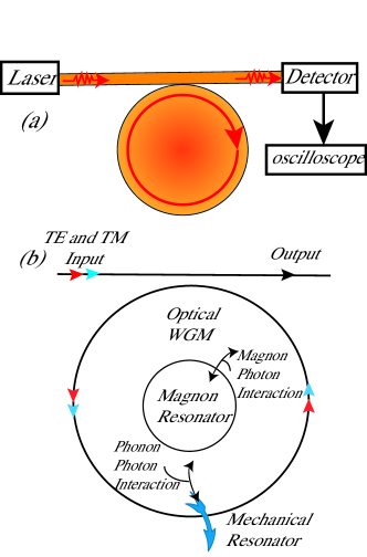
Figure 1: (color online)The structure of the studied system in this article. Fig.(a) shows the consist objects of this system, a glass ball doped with YIG have the mechanical mode. A fiber taper coupled the pumped field with the magnon-phonton-phonon system. In Fig.(b) the interaction scheme is shown. Through the phonon-photon and the magnon-photon interaction. The Magnon and phonon system were bridged. The red and blue arrows show represent the TE and TM pumping respectively.

The effective Hamiltonian under the non-depletion approximation and linearization have the form (The detail deduction can be found in A )

$$H=\omega_{b}\hat{b}^{{\dagger}}\hat{b}+\omega_{m}\hat{m}^{{\dagger}}\hat{m}+\omega_{r}\hat{r}^{{\dagger}}\hat{r}+G_{a}\hat{b}^{{\dagger}}\hat{m}+G_{a}^{*}\hat{b}\hat{m}^{{\dagger}}+G_{b}(\hat{b}^{{\dagger}}+\hat{b})\hat{z},$$ (1)

where $G_{a}=g_{m}<a>=g_{m}\sqrt{2\kappa_{a,1}}a_{in}/(-i(\omega_{L}-\omega_{a})+\kappa_{a})$ is the effective magnon-photon coupling strength, while $G_{b}=g_{b}<b>=g_{b}\sqrt{2\kappa_{b,1}}b_{in}/(-i(\omega_{pu}-\omega_{b})+\kappa_{b})$ is the effective phonon-photon coupling strength. $\omega_{a}$($\omega_{b}$) is the frequency of the TM(TE) mode, $\omega_{m}$ is the magnetic frequency and $\omega_{r}$ is the frequency of the phonon. The $j^{{\dagger}}$($j$) $(j=a,b,m,r)$ is the creation (annihilation) operator of the related mode (TM mode photon, TE mode photon, magnon and phonon). $g_{m}$ describes the interaction strength between the photon and magnon, and $g_{b}$ describes the interaction strength between photon and phonon. $\hat{z}=\hat{r}^{{\dagger}}+\hat{r}$ is the displacement operator of the phonon. Based on the Hamiltonian, we can get the coupling equation on the frequency domain as (B)

$$\chi_{b}^{-1}[\omega]b[\omega] =-iG_{b}z[\omega]-iG_{a}m[\omega],$$ (2a)

$$\chi_{r}^{-1}[\omega]r[\omega] =-i(G_{b}^{*}b[\omega]+G_{b}b^{*}[-\omega])+\sqrt{\gamma_{r}}\eta_{r}[\omega],$$ (2b)

$$\chi_{m}^{-1}[\omega]m[\omega] =-iG_{a}b[\omega]+\sqrt{\gamma_{m}}\eta_{m}[\omega].$$ (2c)

The $\chi[\omega]=(\gamma/2-i(\omega-\omega_{j})),j=b,r,m$ is the intrinsic susceptibility of its corresponding degree of freedom.

III The optical modulation of phonon and magnon interaction

III.1 The mediated self-energy and interaction strength

The case of optically medicated mechanical resonator has been studied previously PhysRevLett.112.013602 . In order to investigate the self-energy of the magnon and the mediated interaction, we eliminate the electromagnetic part $b[\omega]$ of the system and solve the self-energy part of the system. And we neglect the effective interaction terms between the phonon and magneton,

$$(\chi_{m}^{-1}[\omega]+i\Sigma_{mm}[\omega])m[\omega] =\sqrt{\gamma_{m}}\eta_{m}[\omega],$$ (3a)

$$(\chi_{r}^{-1}[\omega]+i\Sigma_{rr}[\omega])z[\omega] =\sqrt{\gamma_{r}}\eta_{r}[\omega],$$ (3b)

where $\Sigma_{rr}[\omega]=-i|G_{b}|^{2}(\chi_{b}[\omega]-\chi_{b}^{*}[-\omega])$ denotes the optomechanical self-energy. Similarly, $\Sigma_{mm}[\omega]=-iG_{a}^{2}\chi_{b}[\omega]$ is defined as the self-energy of the magnon. This self-energy represents the contribution of the optomagnonics to the magnonical resonance frequency $\delta\omega_{i}=\mathrm{Re}(\Sigma_{mm}[\omega_{i}])$ and damping $\delta\gamma_{i}=\mathrm{Im}(\Sigma_{mm}[\omega_{i}]),i=m,r$. Here $G_{a}$ is mediated by the TM pumping field and $\chi_{c}$ can be controlled by the detuning $\Delta_{b}$ of the TE optical pump field.

To study the relationship between the frequency detuning and self-energy, we assume that the $TE$ mode is pumped with the frequency $\omega_{L}=\omega_{b}$ and the magnon resonant with the phonon ($\omega_{r}=\omega_{m}$). By selecting the proper Q-factor, we have the relation $\gamma_{m}=\gamma_{r}=\kappa_{a}=\kappa_{b}=\gamma$. Suppose both the TE and TM modes are under the critical coupling condition as $\kappa_{i,1}=\kappa_{i}/2(i=a,b)$ with the pumping field. Besides, we take $a_{in}g_{m}=b_{in}g_{b}$ to ensure $G_{a}$ is comparable with $G_{b}$. Here we set $\omega_{r}=0.4\gamma$, then the mechanical mode is working on the unresolved-sideband regime.

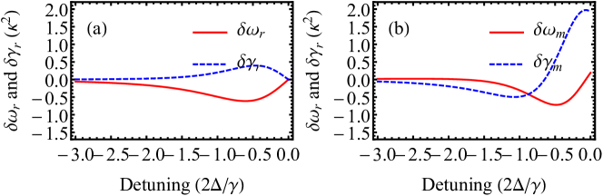
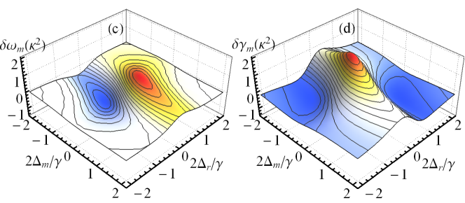
Figure 2: The strength of the self energy as a function of detune. In (a) and (b) we plot the frequency and the damping shift under different monochromatic driving, while in (c) and (d) we respectively plot the frequency and the damping shift of the magnon when the system is driven with different frequency on TM and TE mode. Here the detuning-$\Delta$ is plot in the step of decay $\gamma$. The amplitude of the frequency and the damping shift have a unit of $(g_{i}a_{i}\kappa)^{2}$. Here (a) shows the frequency and damping shift of the mechanical resonator. As symbol in the figure, the red solid line corresponding toe the frequency shift while the blue dash line shows the damping modulation. The figure (b) shows the same subjects of the magnon’s.

To intuitively show the influence of the pump field frequency on the self-energy, we plot the medicated frequency and damping in Fig.2. Compared with the self energy of the mechanical resonator shown in Fig.2(a) PhysRevLett.112.013602 , the self energy of the magnon is different. In Fig.2(b), we plot the monochrome pumped condition (The TM pump frequency is equal to TE pump frequency). It shows the difference of self energy between the magnon and mechanical resonator, both the medicated frequency and the damping of the magnon can be positive and negative valued. In general, the positive and negative frequency detune corresponds to the blue and red shift of the resonator, while for the damping term, the positive and negative mean the resonator work in the gain or dissipative region. So it is shift and damping features tunable for magnon but not for the mechanical resonator. In order to further study the characteristics of the self-energy of the magnon. We plot the 3D-graph to show the influence of the frequency of the TE and TM field. Fig.2(c) shows the frequency shift of the magnon, while in Fig.2(d) we show the dissipation’s variation under different TE and TM pump detuning. As shown in these two figures, the action of the frequency shift and damping change are not synchronization. In this sense, we can independently control the frequency and damping.

The self-energy term shows the interaction between the resonators and the optical field, while the interaction terms provides the interface of the magnon and phonon. To study its influence, we rewrite the Eq.3 with the consideration of the medicated interaction

$$(\chi_{m}^{-1}[\omega] +i\Sigma_{mm}[\omega])m[\omega]=\sqrt{\gamma_{m}}\eta_{m}[\omega]-i\Sigma_{mr}[\omega]z[\omega],$$ (4a)

$$(\chi_{r}^{-1}[\omega] +i\Sigma_{rr}[\omega])z[\omega]=\sqrt{\gamma_{r}}\eta_{r}[\omega]-i\Sigma_{rm}[\omega]m[\omega]+i\Sigma^{*}_{rm}[-\omega]m^{*}[-\omega]).$$ (4b)

Here $\Sigma_{mr}[\omega]=-iG_{a}G_{b}\chi_{b}[\omega]$ and $\Sigma_{rm}[\omega]=-iG_{a}G^{*}_{b}\chi_{b}[\omega]$ are the medicated interaction strength. The coupling has different coupling dissipation. Meanwhile, the $G_{a}$ and $G_{b}$ can be medicated by the TE and TM pumping frequency. Then we can control the interaction strength by modulate the pump field. In order to simplify the results, we set $\omega_{r}=\omega_{m}$, $\gamma_{m}=\gamma_{r}=\kappa_{a}=\kappa_{b}=\gamma$ and $\kappa_{j,1}=\kappa_{j}/2(j=a,b)$.

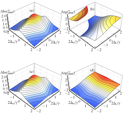
Figure 3: (color online)The real and image part of the medicated coupling strength. We show the $\Sigma_{mr}$ in (a) and (b), while $\Sigma_{rm}$ in (c) and (d). Here (a) and (c) shows the real part, while (b) and (d) shows the image part. Here the detuning-$\Delta$ is plot in the step of decay $\gamma$. The amplitude of the frequency and the damping shift have a unit of $(g_{i}a_{i}\kappa)^{2}$. The subscript $ij$ means the effect of $i$ to $j$ system.

In Fig.3 we respectively plot the strength and phase part of the interaction strength of mechanical resonator to magnon and magnon to mechanical resonator. In the figure, Fig.3(a) and Fig.3(b) show the strength and phase of $\Sigma_{mr}[\omega_{i}]$ respectively, while the strength and phase of $\Sigma_{rm}[\omega_{i}]$ in exhibited in Fig.3(c) and Fig.3(d). It can be easily find that these two coupling strength have the same strength. We know that absolute phase of the interaction will not influence the features of the system. But as shown in Fig.3(b) and Fig.3(d). The coupling phase will be different in most region of this system. Then there will be a relative phase. From Eq.4, we can also elicit that there is a phase difference origin from the $G_{b}$ and $G_{b}^{*}$ term. This relative phase gives us one more freedom to control the system. Even more the generation of this relative phase is also a novel feature of this hybrid system.

III.2 The transverse electric field transmission

To further describe the magnon-phonon system using the electromagnetic field, we first give the expression of the electromagnetic field of the TE mode as

$$b[\omega]= \frac{X[\omega]Y[\omega]X^{*}[-\omega]+X[\omega]}{1-X[\omega]Y[\omega]X^{*}[-\omega]Y^{*}[-\omega]}Z[\omega],$$ (5a)

$$\begin{split}X[\omega]=&(\chi_{b}^{-1}[\omega]+G_{b}^{*}G_{b}(\chi_{r}[\omega]-\chi_{r}^{*}[-\omega])\\ &+G_{a}^{2}\chi_{m}[\omega])^{-1},\end{split}$$ (5b)

$$Y[\omega]= G_{b}^{2}(\chi_{r}[\omega]-\chi_{r}^{*}[-\omega]),$$ (5c)

$$Z[\omega]= -iG_{b}(\chi_{r}[\omega]+\chi_{r}^{*}[-\omega])\sqrt{\gamma_{r}}\eta_{r}-iG_{a}\chi_{m}[\omega]\sqrt{\gamma_{m}}\eta_{m}.$$ (5d)

In these equations, the effective photon-magnon input term $Z[\omega]$ is affected by the environment of the magnentic and mechanical resonator which is described by the expression of the electromagnetic field $b[\omega]$ as shown in Eq.5. Here we take the thermal noise environment as an example to study the feature of this system. The magnetic and mechanical mode of the resonator has the quality factor $Q_{r}=Q_{m}\sim 1\times 10^{3}$. Consider the stochastic and incoherent feature, we assume that

$$S_{Z}[\omega]=\delta_{r,m}Z^{*}[\omega_{1}]Z[\omega].$$ (6)

The thermal noise spectrum is $k_{B}T/\omega$ which could be set as a constant as the change of the frequency ($|\omega_{r}-\omega_{m}|$) is neglectable when compared with the frequency we studied ($\omega_{r},\omega_{m}$). The thermal noise is set as the unit value as the effect of the noise exists on the whole system. Here the two terms $a_{in}g_{m}$ and $b_{in}g_{r}$ are chosen as a whole part. Consider that $a_{in}g_{m}\sim b_{in}g_{r}\sim 1$ THz and $g_{m}\sim 100Hz$ PhysRevLett.117.123605 , $g_{m}\sim 5000Hz$ PhysRevLett.112.013602 and the wavelength is around 1550nm, we can calculate that the TM mode pumping power $P_{m}\sim 20$ mW while the TE pumping power is $P_{r}\sim 7.9\mu$ W. And the damping rate of this system are set as $\kappa_{a}=\kappa_{b}=\kappa_{m}=\kappa_{r}=20$MHz. The magnon and photon have the frequency of $\omega_{m}=1Gz-150$MHz and $\omega_{r}=1$Gz$+150$MHz.

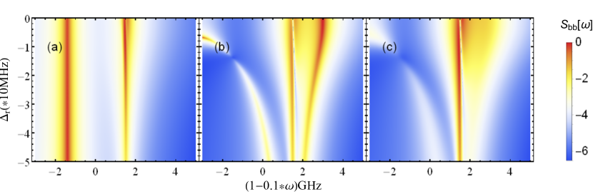
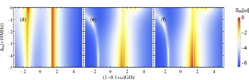
Figure 4: Power spectral density (arbitrary units) of the heterodyne signal. (a)(b) (c)TE and (d)(e)(f)TM as a function of measurement frequency (horizontal axis) and detuning between the incident laser and the cavity resonance (vertical axis). The date in (a) and (d) shows the low effective input power $a_{in}g_{m}=b_{in}g_{r}=0.6$ THz, this power is $a_{in}g_{m}=b_{in}g_{r}=3.6$ THz in figure (b),(c),(e)and (f). In figure (a) and (b) The TM detune is set as $\Delta_{m}=0Hz$ while in (c)$\Delta_{m}=-3MHz$. In figure (d) and (e) The TE detune is set as $\Delta_{m}=0Hz$ while in (f)$\Delta_{m}=-3MHz$.

As the intrinsic susceptibility of the system is sensitive to the frequency, the thermal noise will drive this system effectively on the resonant condition. In this structure, both the pump frequency and the pump power of the electromagnetic field can be modulated, and even the TE and TM field. We further study the system by using the optical spectrum under the influence of the thermal noise in Fig.4. In Fig.4(a), we plot the effective pumping $a_{in}g_{m}=b_{in}g_{r}=0.6$THz, while we set the detuning of the TM pumping field is zero($\Delta_{m}=0$). The thermal noise can be observed in the frequency domain of the TE mode. In this figure, the maximal value of the electromagnetic field corresponds to the condition that the thermal noise resonant with the phonon-magnon system, then the effective frequency of the phonon-magnon hybrid resonator could be readout. While in Fig.4(d), we show the influence of TM detuning on the spectrum.

By increasing the pumping power, the optically-medicated effect becomes obvious. The electromagnetic field works as an optical spring in this condition which connects the phonon and magnon system by producing an effective coupling between them. In order to discuss this strong pumping region, we enlarge this effective driving strength to $a_{in}g_{m}=b_{in}g_{r}=3.6\times 10^{12}$Hz. Fig.4(b)(c) show the influence of the TE pump detuning. In Fig.4(b) the TM detuning is set as $\Delta_{m}=0Hz$, while it is $\Delta_{m}=-3$MHz in Fig.4(c). Three bands could be observed in this system, the magnon band, the phonon band and the optical spring band. The left band corresponds to the magnon mode and there is an obvious frequency shift in the magnon mode. The magnon mode disappears when the detune is bigger than $-10$MHz. It means that the magnon mode becomes a dark mode. The interaction between the magnon mode and the optical field disappears while it interferes with the optical and mechanical hybrid interaction. In Fig.4(c), we can find that the third band obviously changes with a slight detuning of TM mode. We can conclude that the right band can be connected with the optical spring effect.

The influence of TM detuning is shown in Fig.4(e)(f). We can find the third band only can be found in the zero detuning region. In these two figures, the magnon mode is weaker than the phonon mode, and it comes from the relative coupling phase of the magnon-photon to phonon-photon. And we can find both in (e) and (f), the dark magnon state appears when the pumping detune is bigger than $-10$MHz. And when the TM detuning is large enough, the effective frequency shift is not so obvious. It can be explained as when the detune is strong, the magnon is decoupled from this system, then the mognon mode could not be found in the optical field. Different from Fig.4(e) with $\Delta_{r}=0$, Fig.4 (f) is plotted under the detuning $\Delta_{r}=-3$MHz. We can find that this two optical spectrum are identical. The TE detuning only influence the absolute intensity of the field in the plotted region.

IV The topological features of the hybrid phonon-magnon system

IV.1 Topological energy with exceptional points

We consider the system combines the magnon and phonon as a closed system which include an optical pumping. For simplicity, we study the mechanical mode in the phonon mode but not displacement momentum operator. The reduced Hamiltonian can be write as (The detailed derivation can be find in C ),

$$H=\left\{\begin{matrix}\omega_{r}-i\frac{\kappa_{r}}{2}&0\\ 0&\omega_{m}-i\frac{\kappa_{m}}{2}\end{matrix}\right\}\\ -i\left\{\begin{matrix}|G_{b}|^{2}[\chi_{b}[\omega_{m}]-\chi_{b}^{*}[-\omega_{m}]]&G_{a}^{*}G_{b}\chi_{b}[\omega_{m}]\\ G_{a}G_{b}\chi_{b}[\omega_{m}]&G_{a}^{2}\chi_{b}[\omega_{m}]\end{matrix}\right\}.$$ (7)

With the exact diagonalization of the Hamiltonian, two eigenenergies are shown as a function of pumping power and detuning of the TE field in Fig5. This system will possess the exceptional points(EPs) if the system which is tuned at $16|G_{a}|^{2}G_{b}^{2}\chi_{b}^{2}+(2|G_{b}|^{2}(\chi_{b}^{*}-\chi_{b})+2G_{a}^{2}G_{b}+\kappa_{m}-\kappa_{r}+2i(\omega_{m}-\omega_{r}))^{2}=0$. To achieve the equality condition, both the real and image part should be controlled. Fortunately, $G_{a}$ and $G_{b}$ are both pumping frequency and strength dependent, while $\chi_{b}$ can also be controlled by the TE pumping frequency. To simplify this study, we set the TM detuning equal to the TE detuning, even more, the effective pumping rate are set as equal values.

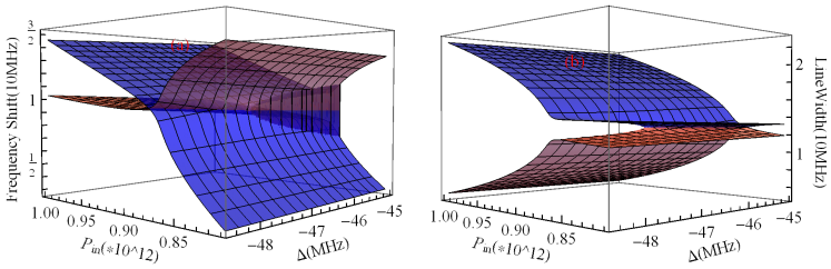
Figure 5: (color online) Then energy scheme of this hybrid system. Figure (a) show the real part (b) is the image part.Here the $P_{in}=a_{in}g_{m}=b_{in}g_{r}$ is the effective input strength, while the $\Delta$ is the frequency detune of the TE mode. The TM mode detune is set as $-3MHz$. We use $\Delta$ to symbol $Delta_{b}$-the TE detune. Here the cavity, magnon and phonon dissipation is $20MHz$. The magnon has the frequency of $1GHz-16MHz$, while it is $1GHz+16MHz$ for the phonon.

In Fig.5, we show the real and imaginary part of the eigenenergy of the medicated Hamiltonian in Eq.7. And we take the parameters shown in last section, except that the magnon frequency is $984$MHz, while the phonon has frequency $1016$MHz. Even more, we fix the value of the TM detuning as $\Delta_{a}=-3$MHz. The input field could be written as the effective form $P_{in}=a_{in}\times g_{m}=b_{in}\times g_{r}$. For the eigenfrequency, we plot its shift from $1$GHz. Here the EPs are obviously in this figure. The two eigenenergy surface of the two super-mode form a Riemann surface, this gives the system a topological feature when the optical pumping encircling with differer direction of the surface. As shown in Fig.5(b), we find the dissipation can be negatively valued. This means the optical field can work as a gain medium, while the gain energy comes from the pumping field.

IV.2 Topological encircling and state evaluation

In order to further study the topological features of this system, we encircling this system under different directions on the Riemann surface. We make this system encircling in a close path, and study the difference when the EPs are included and exclusive in this circle. Take Fig.5 as a reference, we choose the encircling center point as $P_{in}=0.87$THz, $\Delta=-5.5$MHz and $P_{in}=0.87$THz, $\Delta=-4.5$MHz. Here the $P_{in}=a_{in}g_{m}=b_{in}g_{r}$ is the effective input power, while $\Delta$ denotes the frequency detuning of the TE mode. The TM mode detuning is set as $-3$MHz. Here we set the encircling radius as one unit, while one unit is 0.1THz (1MHz) for the $P_{in}$ ($\Delta$) axes. Consider the feature of the topological surface, we also need encircling this system in different directions.

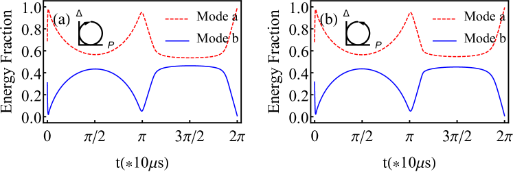
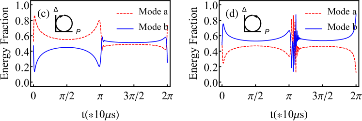
Figure 6: Energy fraction under toplogical encircling. In this figure the effective input power encircling center $P_{in}=a_{in}g_{m}=b_{in}g_{r}=0.87$THz. We use $\Delta$ to symbol $\Delta_{b}$-the TE detune. Here the encircling center in $\Delta$-axes $\Delta=-5.5$MHz for figure (a) and (b), while it is $-4.5$MHz for (c) and (d). (a) and (b) encircling without EP point while (a) and (b) including in it under this setting. The TM mode detune is set as $-3MHz$. The encircling radius is 1 unit. 1 unit is 0.1 THz for the $P_{in}$ axes while for the $\Delta$ axes its $1$MHz. Here the cavity, magnon and phonon dissipation is $20$MHz. The magnon has the frequency of $1$GHz$-16$MHz, while it is $1$GHz$+16$MHz for the phonon. The encircling direction is as shown in the figure.

We plot the energy fraction of mode ”a” and ”b” of the studied system when encircling this system on the Riemann surface. Here mode ”a” corresponds to the red surface of this system, while ”b” corresponds to the blue part. In these figures, we always use the initial mode vectors to project the destiny matrix. Here in Fig.6 (a) and (b), we plot the mode evaluation of the magnon-phonon super-mode when the system encircling with the direction shown in the figure. Also the red line corresponds to mode ”a” while the blue line denotes mode ”b”. Here Fig.6(b) and (d) have an additional phase $\pi$ to make the mode evaluation synchronize with Fig.6(b). Here this system is encircling with the period of $T=10$ms to make sure the system adiabatic evaluation for this system has a frequency of GHz.

Here we analyze the phenomenon shown in Fig.6(a) and (b). In these figures, the encircling region does not include the EP points. We can find the mode evolution almost in the same way. With the adiabatic evaluation, this system shows similar features when encircling in different direction. The tiny difference comes the system stays in different Riemann surface. Different from the above condition, when we include the EP points in the encircling, the evolution of this system will be quite different. As shown in Fig.(c)(d), the difference is that the system will experience an acute oscillation even this system is evolute in a slow way. After the oscillation, there is a crossover between the two energy levels. It means that there is an energy level variation during the evolution. The EP points are work as phase change points as the system feels a sudden energy change when encircling. Moreover, the system is different when it evaluating in different direction. The main differences of the oscillation are the strength and lasting time. It can be attribute to the EP point with chirality when encircling as shown in Fig.5.

V Summary

In summary, we have theoretically investigated the electromagnetic cavity-mediated phonon-magnon interaction system and elaborated how to connect the phonon and magnon mode through the optical medication. As a medium, the electromagnetic field will bring the self-energy and medicate the interaction between the magnon and phonon. When take the thermal noise as an example to study the influence of the environment, we find that the thermal field influences the output of the electromagnetic field. Even more, the magnon will become a dark state when the detune were small. Base on the coupling equations, we investigate the topological features of the hybrid system with the Hamiltonian. When encircling with the EPs on the Riemann energy-surface, the energy level projection shows different vibration behaviour which indicate the chirality of the system.

VI Acknowledgements

The authors gratefully acknowledge the support from the National Natural Science Foundation of China through Grants Nos. 61622103, 61471050 and 61671083; the Ministry of Science and Technology of the People’s Republic of China (MOST) (2016YFA0301304); the Fok Ying-Tong Education Foundation for Young Teachers in the Higher Education Institutions of China (Grant No. 151063); the Open Research Fund Program of the State Key Laboratory of Low-Dimensional Quantum Physics, Tsinghua University Grant No. KF201610. Also we would like to thank Dr. Qi-Kai He for helpful discussions.

Appendix A The effective Hamiltonian of this system 

We input signals, which include both the TE and TM modes, and suppose the coupling strength between TM mode and mechanical mode($g_{a}$) far less than that of TE mode and mechanical mode($g_{b}$), i.e. $g_{a}\ll g_{b}$. In this sense, the Hamiltonian is,

$$H=\omega_{a}\hat{a}^{{\dagger}}\hat{a}+\omega_{b}\hat{b}^{{\dagger}}\hat{b}+\omega_{m}\hat{m}^{{\dagger}}\hat{m}+\omega_{r}\hat{r}^{{\dagger}}\hat{r}+g_{m}(\hat{a}\hat{b}^{{\dagger}}\hat{m}+\hat{a}^{{\dagger}}\hat{b}\hat{m}^{{\dagger}})+g_{b}\hat{b}^{{\dagger}}\hat{b}(\hat{r}^{{\dagger}}+\hat{r}),$$ (8)

where $\omega_{a}$($\omega_{b}$) is the frequency of the TM(TE) mode, $\omega_{m}$ is the magnetic frequency and $\omega_{r}$ is the frequency of the phonon. The $j^{{\dagger}}$($j$) $(j=a,b,m,r)$ is the creation (annihilation) operator of corresponding mode(TM mode photon, TE mode photon, magnon and phonon). $g_{m}$ is the interaction strength of photon and magnon, and $g_{b}$ is the interaction strength of photon and phonon. The TM mode is driven by $\sqrt{2\kappa_{a,1}}a_{in}(\hat{a}e^{i\omega_{L}t}+\hat{a}^{{\dagger}}e^{-i\omega_{L}t})$. $\kappa_{a,1}$ is the coupling damping. $a_{in}$ is the input power and $\omega_{L}$ is the TM pumping frequency. With the non-depletion approximation, the intracavity TM field

$$\langle a\rangle=\frac{\sqrt{2\kappa_{a,1}}a_{in}}{-i(\omega_{L}-\omega_{a})+\kappa_{a}},$$ (9)

where the $\kappa_{a}$ is the total damping of the TM mode of the cavity. The $\langle a\rangle$ corresponds to the interaction enhancement of the interaction between the TE-photon and magnon mode. We write this effective coupling strength as $G_{a}=g_{m}\langle a\rangle$. Then the effective Hamiltonian can be read as

$$H=\omega_{b}\hat{b}^{{\dagger}}\hat{b}+\omega_{m}\hat{m}^{{\dagger}}\hat{m}+\omega_{r}\hat{r}^{{\dagger}}\hat{r}+G_{a}\hat{b}^{{\dagger}}\hat{m}+G_{a}^{*}\hat{b}\hat{m}^{{\dagger}}+g\hat{b}^{{\dagger}}\hat{b}(\hat{r}^{{\dagger}}+\hat{r}).$$ (10)

Linear the optomechanical interaction under the strong red-side band pumping $\sqrt{2\kappa_{b,1}}b_{in}(\hat{b}e^{i\omega_{pu}t}+\hat{b}^{{\dagger}}e^{-i\omega_{pu}t})$. We rotate the system with the steady TE field $\bar{b}$. When omit the term which shift the mechanical resonator’s equilibrium position and high order perturbation, the effective Hamiltonian have the form

$$H=\omega_{b}\hat{b}^{{\dagger}}\hat{b}+\omega_{m}\hat{m}^{{\dagger}}\hat{m}+\omega_{r}\hat{r}^{{\dagger}}\hat{r}+G_{a}\hat{b}^{{\dagger}}\hat{m}+G_{a}^{*}\hat{b}\hat{m}^{{\dagger}}+G_{b}(\hat{b}^{{\dagger}}+\hat{b})\hat{z},$$ (11)

where $\hat{z}=\hat{r}^{{\dagger}}+\hat{r}$. The effective coupling strength $G_{b}=\bar{b}g_{b}=\sqrt{2\kappa_{b,1}}b_{in}/(\kappa-i(\omega_{pu}-\omega_{b}))$. In this Hamiltonian $\hat{b}$ is the perturbation term of the TE field.

Appendix B The coupling strength in the frequency domain 

In common sense, the room-temperature experiment is firmly in the classical regime $\hbar\omega_{a}\gg k_{B}T$, we use a classical analysis. We also disregard all noise on the optical drive, applying the rotating frame of $\omega_{pu}\hat{b}^{{\dagger}}\hat{b}$, we use $\Delta_{r}=\omega_{pu}-\omega_{b}$ for simplicity. Then the kinetic equations of this system can be expressed as

$$\dot{b} =-(\frac{\kappa}{2}-i\Delta_{b})b-iG_{b}z-iG_{a}m,$$ (12a)

$$\dot{r} =-(\frac{\gamma_{r}}{2}+i\omega_{r})r-i(G_{b}^{*}b+G_{b}b^{*})+\sqrt{\gamma_{r}}\eta_{r},$$ (12b)

$$\dot{m} =-(\frac{\gamma_{m}}{2}+i\omega_{m})r-iG_{a}b+\sqrt{\gamma_{m}}\eta_{m}.$$ (12c)

The equation in the frequency domain can be derived with the Fourier transform. Here the magnon and phonon is bathed with thermal fluctuations, the thermal Langevin force $\eta_{i}(t)$ is described by $\langle\eta_{i}(t)\rangle=0$ and $\langle\eta_{j}^{*}(t)\eta_{i}(t)\rangle=\delta_{ij}\delta{t-t^{\prime}}k_{B}T/\hbar\omega_{i}$

$$\chi_{b}^{-1}[\omega]b[\omega] =-iG_{b}z[\omega]-iG_{a}m[\omega],$$ (13a)

$$\chi_{r}^{-1}[\omega]r[\omega] =-i(G_{b}^{*}b[\omega]+G_{b}b^{*}[-\omega])+\sqrt{\gamma_{r}}\eta_{r}[\omega],$$ (13b)

$$\chi_{m}^{-1}[\omega]m[\omega] =-iG_{a}b[\omega]+\sqrt{\gamma_{m}}\eta_{m}[\omega].$$ (13c)

The $\chi[\omega]=(\gamma/2-i(\omega-\omega_{j})),j=b,r,m$ the intrinsic susceptibility of its corresponding degree of freedom.

Appendix C The reduced Hamiltonian 

With rotating wave approximation for $\omega_{r}$ and $\omega_{m}$. Eliminate the electromagnetic freedom. Eq.4 in the main text can be written as,

$$\chi_{r}^{-1}[\omega]r[\omega]= -|G_{b}|^{2}[\chi_{b}[\omega]-\chi_{b}^{*}[-\omega]]r[\omega]-G_{a}^{*}G_{b}\chi_{b}[\omega]m[\omega],$$ (14a)

$$\chi_{m}^{-1}[\omega]m[\omega]= -G_{a}^{2}\chi_{b}[\omega]r[\omega]-G_{a}G_{b}\chi_{b}[\omega]r[\omega].$$ (14b)

As a closed system, we discard the thermal noise term. And it can be achieved by putting this system in the low temperature environment. In this two mode system we define the self-energy as

$$\mathbf{\Sigma}[\omega]=-i\left\{\begin{matrix}|G_{b}|^{2}[\chi_{b}[\omega]-\chi_{b}^{*}[-\omega]]&G_{a}^{*}G_{b}\chi_{b}[\omega]\\ G_{a}G_{b}\chi_{b}[\omega]&G_{a}^{2}\chi_{b}[\omega]\end{matrix}\right\}.$$ (15)

When combine the phonon and magnon as a whole vector $\mathbf{s}(t)=(r(t),m(t))^{T}$. Then the system can be written in the matrix form,

$$-i\omega\mathbf{s}[\omega]=-\left\{\begin{matrix}\frac{\kappa_{r}}{2}+i\omega_{r}&0\\ 0&\frac{\kappa_{m}}{2}+i\omega_{m}\end{matrix}\right\}\mathbf{s}[\omega]-i\mathbf{\Sigma}[\omega]\mathbf{s}[\omega].$$ (16)

It is noticeable that $\mathbf{\Sigma}[\omega]$ various on the scale of $\gamma$. whereas this vector modes are susceptible to drives only if their is substantially smaller than $\gamma$. Therefore, it is sufficient to consider $\mathbf{\Sigma}[\omega]\approx\mathbf{\Sigma}[\omega_{r}]\approx\mathbf{\Sigma}[\omega_{m}]\equiv\mathbf{\Sigma}$. Then self-energy is frequency independence. So we can easily move back to the time domain to get the effective schrődinger’s equation,

$$i\dot{\mathbf{s}}(t)=H\mathbf{s}(t).$$ (17)

Here the Hamiltonian reads,

$$H=\left\{\begin{matrix}\omega_{r}-i\frac{\kappa_{r}}{2}&0\\ 0&\omega_{m}-i\frac{\kappa_{m}}{2}\end{matrix}\right\}+\mathbf{\Sigma}.$$ (18)

References

References

- (1) Warwick P and Gerard J 2016 Quantum optomechanics (CRC Press) URL https://www.crcpress.com/Quantum-Optomechanics/Bowen-Milburn/p/book/9781482259155
- (2) Aspelmeyer M, Kippenberg T and Marquardt F 2014 Rev. Mod. Phys. 86(4) 1391–1452 URL http://link.aps.org/doi/10.1103/RevModPhys.86.1391
- (3) Aspelmeyer M, Kippenberg T and Marquardt F 2014 Cavity Optomechanics: Nano- and Micromechanical Resonators Interacting with Light 1st ed Quantum Science and Technology (Springer-Verlag Berlin Heidelberg) URL http://www.springer.com/gp/book/9783642553110
- (4) Kippenberg T and Vahala K 2007 Opt. Express 15 17172–17205 URL http://www.opticsexpress.org/abstract.cfm?URI=oe-15-25-17172
- (5) Peng B, Özdemir Ş K, Chen W, Nori F and Yang L 2014 Nature communications 5 5082 URL http://www.nature.com/articles/ncomms6082
- (6) Anetsberger G, Arcizet O, Unterreithmeier Q P, Rivière R, Schliesser A, Weig E M, Kotthaus J P and Kippenberg T J 2009 Nature Physics 5 909–914 URL http://www.nature.com/nphys/journal/v5/n12/abs/nphys1425.html
- (7) Kippenberg T and Vahala K 2008 Science 321 1172–1176 URL http://science.sciencemag.org/content/321/5893/1172
- (8) Hill J T, Safavi-Naeini A H, Chan J and Painter O 2012 Nature communications 3 1196 URL http://www.nature.com/articles/ncomms2201
- (9) Liu Y C, Xiao Y F, Luan X and Wong C W 2013 Phys. Rev. Lett. 110(15) 153606 URL http://link.aps.org/doi/10.1103/PhysRevLett.110.153606
- (10) Corbitt T, Chen Y, Innerhofer E, Müller-Ebhardt H, Ottaway D, Rehbein H, Sigg D, Whitcomb S, Wipf C and Mavalvala N 2007 Phys. Rev. Lett. 98(15) 150802 URL http://link.aps.org/doi/10.1103/PhysRevLett.98.150802
- (11) Thompson J, Zwickl B, Jayich A, Marquardt F, Girvin S and Harris J 2008 Nature 452 72–75 URL http://www.nature.com/nature/journal/v452/n7183/abs/nature06715.html
- (12) Zhang X, Zou C L, Jiang L and Tang H X 2014 Phys. Rev. Lett. 113(15) 156401 URL http://link.aps.org/doi/10.1103/PhysRevLett.113.156401
- (13) Liu T, Zhang X, Tang H X and Flatté M E 2016 Phys. Rev. B 94(6) 060405 URL http://link.aps.org/doi/10.1103/PhysRevB.94.060405
- (14) Zhang X, Zhu N, Zou C L and Tang H X 2016 Phys. Rev. Lett. 117(12) 123605 URL http://link.aps.org/doi/10.1103/PhysRevLett.117.123605
- (15) Haigh J, Langenfeld S, Lambert N, Baumberg J, Ramsay A, Nunnenkamp A and Ferguson A 2015 Phys. Rev. A 92(6) 063845 URL http://link.aps.org/doi/10.1103/PhysRevA.92.063845
- (16) Bourhill J, Kostylev N, Goryachev M, Creedon D and Tobar M 2016 Phys. Rev. B 93(14) 144420 URL http://link.aps.org/doi/10.1103/PhysRevB.93.144420
- (17) Osada A, Hisatomi R, Noguchi A, Tabuchi Y, Yamazaki R, Usami K, Sadgrove M, Yalla R, Nomura M and Nakamura Y 2016 Phys. Rev. Lett. 116(22) 223601 URL http://link.aps.org/doi/10.1103/PhysRevLett.116.223601
- (18) Haigh J, Nunnenkamp A, Ramsay A and Ferguson A 2016 Phys. Rev. Lett. 117(13) 133602 URL http://link.aps.org/doi/10.1103/PhysRevLett.117.133602
- (19) Viola Kusminskiy S, Tang H X and Marquardt F 2016 Phys. Rev. A 94(3) 033821 URL http://link.aps.org/doi/10.1103/PhysRevA.94.033821
- (20) Kłos J W, Krawczyk M, Dadoenkova Y S, Dadoenkova N and Lyubchanskii I 2014 Journal of Applied Physics 115 174311 URL "http://scitation.aip.org/content/aip/journal/jap/115/17/10.1063/1.4874797"
- (21) Chumak A, Vasyuchka V, Serga A and Hillebrands B 2015 Nature Physics 11 453–461 URL http://www.nature.com/nphys/journal/v11/n6/abs/nphys3347.html
- (22) Tabuchi Y, Ishino S, Noguchi A, Ishikawa T, Yamazaki R, Usami K and Nakamura Y 2015 Science 349 405–408 URL http://science.sciencemag.org/content/349/6246/405
- (23) Huebl H, Zollitsch C W, Lotze J, Hocke F, Greifenstein M, Marx A, Gross R and Goennenwein S T 2013 Phys. Rev. Lett. 111(12) 127003 URL http://link.aps.org/doi/10.1103/PhysRevLett.111.127003
- (24) Brooks D W, Botter T, Schreppler S, Purdy T P, Brahms N and Stamper-Kurn D M 2012 Nature 488 476–480 URL http://www.nature.com/nature/journal/v488/n7412/abs/nature11325.html
- (25) Safavi-Naeini A H, Gröblacher S, Hill J T, Chan J, Aspelmeyer M and Painter O 2013 Nature 500 185–189 URL http://www.nature.com/nature/journal/v500/n7461/abs/nature12307.html
- (26) Purdy T P, Yu P L, Peterson R W, Kampel N S and Regal C A 2013 Phys. Rev. X 3(3) 031012 URL http://link.aps.org/doi/10.1103/PhysRevX.3.031012
- (27) Liao J Q and Law C K 2011 Phys. Rev. A 83(3) 033820 URL http://link.aps.org/doi/10.1103/PhysRevA.83.033820
- (28) Nunnenkamp A, Børkje K, Harris J G E and Girvin S M 2010 Phys. Rev. A 82(2) 021806 URL http://link.aps.org/doi/10.1103/PhysRevA.82.021806
- (29) Arcizet O, Cohadon P F, Briant T, Pinard M, Heidmann A, Mackowski J M, Michel C, Pinard L, Français O and Rousseau L 2006 Phys. Rev. Lett. 97(13) 133601 URL http://link.aps.org/doi/10.1103/PhysRevLett.97.133601
- (30) Tsang M and Caves C M 2010 Phys. Rev. Lett. 105(12) 123601 URL http://link.aps.org/doi/10.1103/PhysRevLett.105.123601
- (31) Teufel J, Donner T, Castellanos-Beltran M, Harlow J and Lehnert K 2009 Nature nanotechnology 4 820–823 URL http://www.nature.com/nnano/journal/v4/n12/abs/nnano.2009.343.html
- (32) Nimmrichter S, Hornberger K and Hammerer K 2014 Phys. Rev. Lett. 113(2) 020405 URL http://link.aps.org/doi/10.1103/PhysRevLett.113.020405
- (33) Shkarin A B, Flowers-Jacobs N E, Hoch S W, Kashkanova A D, Deutsch C, Reichel J and Harris J G E 2014 Phys. Rev. Lett. 112(1) 013602 URL http://link.aps.org/doi/10.1103/PhysRevLett.112.013602
- (34) Weis S, Rivière R, Deléglise S, Gavartin E, Arcizet O, Schliesser A and Kippenberg T J 2010 Science 330 1520–1523 URL http://science.sciencemag.org/content/330/6010/1520
- (35) Monifi F, Zhang J, Özdemir Ş K, Peng B, Liu Y x, Bo F, Nori F and Yang L 2016 Nature Photonics 399––405 URL http://www.nature.com/nphoton/journal/v10/n6/full/nphoton.2016.73.html
- (36) Safavi-Naeini A H, Alegre T M, Chan J, Eichenfield M, Winger M, Lin Q, Hill J T, Chang D E and Painter O 2011 Nature 472 69–73 URL http://www.nature.com/nature/journal/v472/n7341/abs/nature09933.html
- (37) Jing H, Özdemir Ş K, Geng Z, Zhang J, Lü X Y, Peng B, Yang L and Nori F 2015 Scientific reports 5 9663 URL http://www.nature.com/articles/srep09663
- (38) Stannigel K, Komar P, Habraken S J M, Bennett S D, Lukin M D, Zoller P and Rabl P 2012 Phys. Rev. Lett. 109(1) 013603 URL http://link.aps.org/doi/10.1103/PhysRevLett.109.013603
- (39) Wang Y D and Clerk A A 2012 New Journal of Physics 14 105010 URL http://stacks.iop.org/1367-2630/14/i=10/a=105010
- (40) Liu Y C, Xiao Y F, Chen Y L, Yu X C and Gong Q 2013 Phys. Rev. Lett. 111(8) 083601 URL http://link.aps.org/doi/10.1103/PhysRevLett.111.083601
- (41) Ludwig M, Safavi-Naeini A H, Painter O and Marquardt F 2012 Phys. Rev. Lett. 109(6) 063601 URL http://link.aps.org/doi/10.1103/PhysRevLett.109.063601
- (42) Serga A A, Chumak A V and Hillebrands B 2010 Journal of Physics D: Applied Physics 43 264002 URL http://stacks.iop.org/0022-3727/43/i=26/a=264002
- (43) Montagnese M, Otter M, Zotos X, Fishman D A, Hlubek N, Mityashkin O, Hess C, Saint-Martin R, Singh S, Revcolevschi A and van Loosdrecht P H M 2013 Phys. Rev. Lett. 110(14) 147206 URL http://link.aps.org/doi/10.1103/PhysRevLett.110.147206
- (44) Lenk B, Ulrichs H, Garbs F and Münzenberg M 2011 Physics Reports 507 107–136 URL http://www.sciencedirect.com/science/article/pii/S0370157311001694
- (45) Cowburn R P and Welland M E 2000 Science 287 1466–1468 URL http://science.sciencemag.org/content/287/5457/1466
- (46) Imre A, Csaba G, Ji L, Orlov A, Bernstein G H and Porod W 2006 Science 311 205–208 URL http://science.sciencemag.org/content/311/5758/205
- (47) Tanji H, Ghosh S, Simon J, Bloom B and Vuletić V 2009 Phys. Rev. Lett. 103(4) 043601 URL http://link.aps.org/doi/10.1103/PhysRevLett.103.043601
- (48) Lorenzana J and Sawatzky G A 1995 Phys. Rev. Lett. 74(10) 1867–1870 URL http://link.aps.org/doi/10.1103/PhysRevLett.74.1867
- (49) Zhang X, Zou C L, Zhu N, Marquardt F, Jiang L and Tang H X 2015 Nature communications 6 8914 URL http://www.nature.com/articles/ncomms9914
- (50) Armani D, Kippenberg T, Spillane S and Vahala K 2003 Nature 421 925–928 URL http://www.nature.com/nature/journal/v421/n6926/abs/nature01371.html
- (51) Vahala K J 2003 Nature 424 839–846 URL http://www.nature.com/nature/journal/v424/n6950/abs/nature01939.html
- (52) Gorodetsky M L and Ilchenko V S 1999 JOSA B 16 147–154 URL https://www.osapublishing.org/josab/abstract.cfm?uri=josab-16-1-147
- (53) Kushida T 2000 Magneto-Optics 1st ed Springer Series in Solid-State Sciences 128 (Springer-Verlag Berlin Heidelberg)
- (54) Bennett H S and Stern E A 1965 Phys. Rev. 137(2A) A448–A461 URL http://link.aps.org/doi/10.1103/PhysRev.137.A448
- (55) Inoue M and Fujii T 1997 Journal of applied physics 81 5659–5661 URL http://scitation.aip.org/content/aip/journal/jap/81/8/10.1063/1.364687
- (56) Kirilyuk A, Kimel A V and Rasing T 2010 Rev. Mod. Phys. 82(3) 2731–2784 URL http://link.aps.org/doi/10.1103/RevModPhys.82.2731
- (57) Kimel A, Kirilyuk A, Usachev P, Pisarev R, Balbashov A and Rasing T 2005 Nature 435 655–657 URL http://www.nature.com/nature/journal/v435/n7042/abs/nature03564.html
- (58) Demokritov S, Hillebrands B and Slavin A 2001 Physics Reports 348 441 – 489 URL http://www.sciencedirect.com/science/article/pii/S0370157300001162
- (59) Fleury P A and Loudon R 1968 Phys. Rev. 166(2) 514–530 URL http://link.aps.org/doi/10.1103/PhysRev.166.514
- (60) Gorodetsky M and Ilchenko V 1994 Optics Communications 113 133 – 143 URL http://www.sciencedirect.com/science/article/pii/0030401894906033