Symmetries and choreographies in families bifurcating from
the polygonal relative equilibrium of the $n$-body problem

Abstract

We use numerical continuation and bifurcation techniques in a boundary value setting to follow Lyapunov families of periodic orbits. These arise from the polygonal system of $n$ bodies in a rotating frame of reference. When the frequency of a Lyapunov orbit and the frequency of the rotating frame have a rational relationship then the orbit is also periodic in the inertial frame. We prove that a dense set of Lyapunov orbits, with frequencies satisfying a diophantine equation, correspond to choreographies. We present a sample of the many choreographies that we have determined numerically along the Lyapunov families and along bifurcating families, namely for the cases $n=4,~{}6,~{}7,~{}8$, and $9$. We also present numerical results for the case where there is a central body that affects the choreography, but that does not participate in it. Animations of the families and the choreographies can be seen at the link below.

Introduction

The study of $n$ equal masses that follow the same path has attracted much attention in recent years. The first solution that differs from the classical Lagrange circular one was discovered numerically by C. Moore in 1993 [24], where three bodies follow one another around the now famous figure-eight orbit. This orbit was located by minimizing the action among symmetric paths. Independently in [7], Chenciner and Montgomery (2000) gave a rigorous mathematical proof of the existence of this orbit, by minimizing the action over paths that connect a colinear and an isosceles configuration. Such solutions are now commonly known as “choreographies”, after the work in [27], where C. Simó presented extensive numerical computations of choreographies for many choices of the number of bodies.

The results in [7] mark the beginning of the development of variational methods, where the existence of choreographies can be associated with the problem of finding critical points of the classical action of the Newton equations of motion. The main obstacles encountered in the application of the principle of least action are the existence of paths with collisions, and the lack of compactness of the action. In [13], Terracini and Ferrario (2004) applied the principle of least action systematically over symmetric paths to avoid collisions, using ideas introduced by Marchal [21]. For the discussion of these and other variational approaches we refer to [2, 3, 11, 12, 28], and references therein.

Another way to obtain choreographies is by using continuation methods. Chenciner and Féjoz (2009) pointed out in [4] that choreographies appear in dense sets along the Vertical Lyapunov families that arise from $n$ bodies rotating in a polygon; see also [5, 15, 20]. The local existence of the Vertical Lyapunov families is proven in [4] using the Weinstein-Moser theory. When the frequency varies along the Vertical Lyapunov families then an infinite number of choreographies exists; a fact established in [4] for orbits close to the polygon equilibrium, with $n\leq 6$. While similar computations can be carried out for other values of $n$, a general analytical proof that is valid for all $n$ remains an open problem.

In [15] C. García-Azpeitia and J. Ize (2013) proved the global existence of bifurcating Planar and Vertical Lyapunov families, using the equivariant degree theory from [16]. The purpose of our current work is to compute such global families numerically, as well as subsequently bifurcating families. To explain our numerical results in a precise notational setting we first recall some relevant results from [15].

The equations of motion of $n$ bodies of unit mass in a rotating frame are given by

$$\ddot{u}_{j}+2\sqrt{s_{1}}~{}i~{}\dot{u}_{j} =s_{1}u_{j}-\sum_{i=1(i\neq j)}^{n}\frac{u_{j}-u_{i}}{\left\|(u_{j},z_{j})-(u_{i},z_{i})\right\|^{3}}~{},$$ (1)

$$\ddot{z}_{j} =-\sum_{i=1(i\neq j)}^{n}\frac{z_{j}-z_{i}}{\left\|(u_{j},z_{j})-(u_{i},z_{i})\right\|^{3}}~{},$$

where the $(u_{j},z_{j})\in\mathbb{C}\times\mathbb{R}$ are the positions of the bodies in space, and $s_{1}$ is defined by

$$s_{k}=\frac{1}{4}\sum_{j=1}^{n-1}\frac{\sin^{2}(kj\zeta/2)}{\sin^{3}(j\zeta/2)}~{},\qquad\zeta=\frac{2\pi}{n}~{}.$$ (2)

The circular, polygonal relative equilibrium consists of the positions

$$u_{j}=e^{ij\zeta},\qquad z_{j}=0\text{.}$$ (3)

The frequency of the rotational frame is chosen to be $\sqrt{s_{1}}$, so that the polygon (3) is an equilibrium of (1). The emanating Lyapunov families have starting frequencies that are equal to the natural modes of oscillation of the equilibrium (3). These Lyapunov families constitute continuous families in the space of renormalized $2\pi$-periodic functions. The global property means that the norm or the period of the orbits along the family tends to infinity, or that the family ends in a collision or at a bifurcation orbit.

The theorem in [15] states that for $n\geq 6$ and for each integer $k$ such that

$$3\leq k\leq n-3,$$

the polygonal relative equilibrium has one global bifurcation of planar periodic solutions with symmetries

$$u_{j}(t)=e^{ij\zeta}u_{n}(t+jk\zeta),\qquad u_{n}(t)=\bar{u}_{n}(-t)\text{.}$$ (4)

Moreover, the proof in [15] predicts solutions with $k=2$ or $n-2$ if the linear equations at the polygonal equilibrium have normal modes corresponding to these symmetries. In fact, three cases occur for different values of $n$: for $n=4,5,6$ there are no solutions with $k=2$ or $n-2$, for $n=7,8,9$ there are two solutions with $k=2$ and no solutions with $k=$ $n-2$, and for $n\geq 10$ there is one solution with $k=2$ and one with $k=$ $n-2$.

In the case of spatial Lyapunov families the eigenvalues of the linearized system of equations are given explicitly by $i\sqrt{s_{k}}$, for $k=1,...,n-1$; see [4] and [15]. The eigenvalues $i\sqrt{s_{k}}$ are resonant due to the fact that $s_{n-k}=s_{k}$ for $1\leq k<n/2$. Moreover, the first eigenvalue $i\sqrt{s_{1}}$ is resonant with the triple planar eigenvalue $i\sqrt{s_{1}}$, and hence is highly degenerate. These resonances can be dealt with using the equivariant degree theory in [16].

The theorem in [15] states that for $n\geq 3$ and for each $k$ such that

$$1\leq k\leq n/2\text{,}$$

the polygonal relative equilibrium has one global bifurcation of spatial periodic solutions, which start with frequency $\sqrt{s_{k}}$, have the symmetry (4), as well as the symmetries

$$z_{j}(t)=z_{n}(t+jk\zeta),$$ (5)

and

$$u_{n}(t)=u_{n}(t+\pi),\qquad z_{n}(t)=-z_{n}(t+\pi).$$ (6)

For example, for the case where $k=n/2$ and $n$ is even, we have $k\zeta=\pi$. Then the symmetries (4), (5) and (6) imply that

$$u_{j}(t) =e^{ij\zeta}u_{n}(t+j\pi)=e^{ij\zeta}u_{n}(t),$$

$$z_{j}(t) =z_{n}(t+jk\zeta)=(-1)^{j}z_{n}(t).$$

Solutions having these symmetries are known as Hip-Hop orbits, and have been studied in [1, 8, 22, 28].

Solutions with symmetries (4) and (5) are “traveling waves”  in the sense that each body follows the same path, but with a rotation and a time shift. The symmetries allow us to establish that a dense set of solutions along the family are choreographies in the inertial frame of reference.

We say that a planar or spatial Lyapunov orbit is $\ell:m$ resonant if its period and frequency are

$$T=\frac{2\pi}{\sqrt{s_{1}}}\left(\frac{\ell}{m}\right)\text{,\qquad}\nu=\sqrt{s_{1}}\frac{m}{\ell}\text{,}$$

where $\ell$ and $m$ are relatively prime, and such that

$$k\ell-m\in n\mathbb{Z}.$$

In Theorem 5 we prove that $\ell:m$ resonant Lyapunov orbits are choreographies in the inertial frame. Each of the integers $k$, $\ell$, and $m$ plays a different role in the description of the choreographies. Indeed, the projection of the choreography onto the $xy$-plane has winding number $\ell$ around a center, and is symmetric with respect to the $\mathbb{Z}_{m}$-group of rotations by $2\pi/m$. In addition the $n$ bodies form groups of $d$-polygons, where $d$ is the greatest common divisor of $k$ and $n$.

Some choreographies wind around a toroidal manifold with winding numbers $\ell$ and $m$, i.e., the choreography path is a $(\ell,m)$-torus knot. In particular, such orbits appear in families that we refer to as ”Axial families”, e.g., in Figure 8. In [2] and [25] different classifications for the symmetries of planar choreographies have been presented. These classifications differ from the one presented here since they are designed for choreographies found by means of a variational approach. The nature of our approach is continuation and as such, the winding numbers $\ell$ and $m$ appear in a natural manner in the classification of the choreographies. Therefore, our approach presents complementary information not available with variational methods. We note that for other values of $\ell$ and $m$ the orbits of the $n$ bodies in the inertial frame are also closed, but consist of multiple curves, called “multiple choreographic solutions” in [3].

We use robust and highly accurate boundary value techniques with adaptive meshes to continue the Lyapunov families. An extensive collection of python scripts that reproduce the results reported in this article for a selection of values of $n$ will be made freely available. These scripts control the software AUTO to carry out the necessary sequences of computations. Similar scripts will be available for related problems, including an $n$ vortex problem and a periodic lattice of Schrödinger sites.

In [4] the numerical continuation of the Vertical Lyapunov families is implemented as local minimizers in subspaces of symmetric paths. Presumably not all families are local minimizers restricted to subspaces. One advantage of our procedure is that it allows the numerical continuation of all Planar and Vertical Lyapunov families that arise from simple eigenvalues. The systematic computation of periodic orbits that arise from eigenvalues of higher multiplicity remains under investigation. Previous numerical work has established the existence of many choreographies; see for example [6]. Computer-assisted proofs of the existence of choreographies have been given in, for example, [17] and [18]. It would be of interest to use such techniques to mathematically validate the existence of some of the choreographies in our article. The figure-8 orbit is still the only choreography known to be stable [18], and so far we have not found evidence of other stable choreographies.

In Section 1 we prove that a dense set of orbits along the Lyapunov families corresponds to choreographies. In Section 2 we describe the numerical continuation procedure used to determine the periodic solution families, and in Section 3 we give examples of numerically computed Lyapunov families and some of their bifurcating families. In Section 4 we provide a sample of the choreographies that appear along Planar Lyapunov families. Section 5 presents choreographies along the Vertical Lyapunov families and along their bifurcating families. In particular, a family of axially symmetric orbits forms a connection between a Vertical family and a Planar family. Choreographies along such tertiary Planar families are referred to as “unchained polygons” in [4].

In Section 6 we present results for a similar configuration, namely the Maxwell relative equilibrium, where a central body is added at the center of the $n$-polygon. This configuration has been used as a model to study the stability of the rings of Saturn, as established in [23] and in [15, 29, 26] for $n\geq 7$. Using a similar approach as in the earlier sections, we determine solutions where $n$ bodies of equal mass $1$ follow a single trajectory, but with an additional body of mass $\mu$ at or near the center. While this extra body does not participate in the choreography, it does affect its structure, and its stability properties. We also present Vertical Lyapunov families that bifurcate from a non-circular, polygonal equilibrium, whose solutions have symmetries that correspond to “standing waves”, and which do not give rise to choreographies in the inertial frame.

1 Choreographies and Lyapunov Families

In this section we prove that there are Lyapunov orbits of the $n$ body problem that correspond to choreographies in the inertial frame of reference.

Lemma 1

Let

$$\Omega=\frac{1}{n}\left(k\frac{\sqrt{s_{1}}}{\nu}-1\right)\text{.}$$

Then in the inertial frame of reference, with period scaled to $2\pi$, the Planar Lyapunov orbits satisfy

$$q_{j}(t)=e^{-ij(2\pi)\Omega}q_{n}(t+jk\zeta).$$

Proof. : In the inertial frame the solutions are given by

$$q_{j}(t)=e^{i\sqrt{s_{1}}t}u_{j}(\nu t),$$

where $\nu$ is the frequency and $T=2\pi/\nu$ is the period. Reparametrizing time the solution becomes $q_{j}(t)=e^{it\sqrt{s_{1}}/\nu}u_{j}(t)$, where $u_{j}$ is the $2\pi$-periodic solution with the symmetries (4). We have

$$q_{j}(t)=e^{it\sqrt{s_{1}}/\nu}u_{j}(t)=e^{it\sqrt{s_{1}}/\nu}e^{ij\zeta}u_{n}(t+jk\zeta)\text{.}$$

Since

$$q_{n}(t+jk\zeta)=e^{i(t+jk\zeta)\sqrt{s_{1}}/\nu}u_{n}(t+jk\zeta)\text{,}$$

it follows that

$$q_{j}(t)=e^{it\sqrt{s_{1}}/\nu}e^{ij\zeta}\left(e^{-i(t+jk\zeta)\sqrt{s_{1}}/\nu}q_{n}(t+jk\zeta)\right)=e^{-ij\zeta n\Omega}q_{n}(t+jk\zeta).$$

 

In particular, if $\Omega\in\mathbb{Z}$ then the Lyapunov solutions satisfy

$$q_{j}(t)=q_{n}(t+jk\zeta)\text{,}$$ (7)

and are choreographies. In fact, planar choreographies exists for any rational number $\Omega=p/q$ where $q$ is relatively prime to $n$.

Proposition 2

If $\Omega=p/q$, with $q$ relatively prime to $n$, then

$$q_{j}(t)=q_{n}(t+j\left(1_{n}k\zeta\right))\text{,}$$ (8)

where $1_{n}=1$ mod $n$. The solution $q_{n}(t)$ is $2\pi m$-periodic, where $m$ and $\ell$ are relatively prime such that

$$\frac{\ell}{m}=\frac{np+q}{kq}\text{.}$$ (9)

Proof. : If $\Omega=p/q$, the solution satisfies

$$q_{j}(t)=e^{-i2\pi jp/q}q_{n}(t+jk\zeta).$$ (10)

Since $n$ and $q$ are relatively prime, we can define $q^{\ast}$ as the modular inverse of $q$. Setting $1_{n}=q^{\ast}q$, there is an $\ell$ such that $j1_{n}=j+n\ell$ for any $j$. Then we have

$$q_{j}(t)=q_{j+n\ell}(t)=e^{-i2\pi(j1_{n}p/q}q_{n}(t+j(1_{n}k\zeta))=e^{-i2\pi(jq^{\ast}p)}q_{n}(t+j(1_{n}k\zeta))\text{.}$$ (11)

Since

$$\frac{\sqrt{s_{1}}}{\nu}=\frac{n\Omega+1}{k}=\frac{np+q}{qk}=\frac{\ell}{m}\text{,}$$

it follows that $e^{it\sqrt{s_{1}}/\nu}$ is $2\pi m$-periodic, and since $u_{n}(t)$ is $2\pi$-periodic, we also have that the function $q_{n}(t)=e^{it\sqrt{s_{1}}/\nu}u_{n}(t)$ is $2\pi m$-periodic.

 

Proposition 3

For $\Omega=p/q$, with $q$ and $n$ relatively prime, the spatial Lyapunov solution is a choreography that satisfies

$$(q_{j},z_{j})(t)=(q_{n},z_{n})(t+j(1_{n}k\zeta))\text{,}$$ (12)

where $1_{n}=1$ mod $n$ and $(q_{j},z_{j})(t)$ is $2\pi m$-periodic.

Proof. : For the planar component of the spatial Lyapunov families we have $q_{j}(t)=q_{n}(t+j1_{n}k\zeta)$, where $q_{n}(t)$ is $2\pi m$-periodic. We have in addition that the spatial component $z_{n}$ is $2\pi$-periodic and satisfies $z_{j}(t)=z_{n}(t+jk\zeta)$. Since $1_{n}=1$ mod $n$, we have

$$z_{j}(t)=z_{n}(t+jk\zeta)=z_{n}(t+j1_{n}k\zeta),$$

where $z_{n}(t)$ is also $2\pi m$-periodic.

 

For fixed $n$ the set of rational numbers $p/q$ such that $q$ and $n$ are relatively prime is dense. If the range of the frequency $\nu$ along the Lyapunov family contains an interval, then there is a dense set of rational numbers $\Omega=p/q$ inside that interval. Hence there is an infinite number of Lyapunov orbits that correspond to choreographies. To be precise, the resonant Lyapunov orbit gives a choreography that has period

$$mT=m\frac{2\pi}{\nu}=\frac{2\pi}{\sqrt{s_{1}}}\ell~{}\text{,}$$

where $T$ is the period of the resonant Lyapunov orbit. Furthermore, the number $\ell$ is related to the number of times that the orbit of the choreography winds around a central point. Rational numbers $p/q$, where $q$ is relatively prime to $n$, appear infinitely often in an interval, with $p$ and $q$ arbitrarily large. In such a frequency interval the infinite number of rationals $p/q$ that correspond to choreographies give arbitrarily large $\ell$ and $m$ as well. This gives rise to an infinite number of choreographies, with arbitrarily large frequencies $\frac{2\pi}{\sqrt{s_{1}}}\ell$, and orbits of correspondingly increasing complexity.

Although the previous results give sufficient conditions for the existence of infinitely many choreographies, there can be additional choreographies due to the fact that the orbit of the choreography $q_{n}(t)$ has additional symmetries by rotations of $2\pi/m$. We now describe these symmetries and the necessary conditions.

Definition 4

We define a Lyapunov orbit as being $\ell:m$ resonant if it has period

$$T_{\ell:m}=\frac{2\pi}{\sqrt{s_{1}}}\frac{\ell}{m}\text{,}$$

where $\ell$ and $m$ are relatively prime such that

$$k\ell-m\in n\mathbb{Z}\text{.}$$

Theorem 5

In the inertial frame an $\ell:m$ resonant Lyapunov orbit is a choreography,

$$(q_{j},z_{j})(t)=(q_{n},z_{n})(t+j\tilde{k}\zeta)\text{,}$$

where $\tilde{k}=k-(k\ell-m)\ell^{\ast}$ with $\ell^{\ast}$ the $m$-modular inverse of $\ell$. The projection on the $xy$-plane of the choreography is symmetric by rotations of the angle $2\pi/m$ and winds around a center $\ell$ times. The period of the choreography is $m~{}T_{\ell:m}$.

Proof. : Since $u_{n}(t)$ is $2\pi$-periodic and

$$e^{it\sqrt{s_{1}}/\nu}=e^{it\ell/m}$$

is $2\pi m$-periodic, the function $q_{n}(t)=e^{it\sqrt{s_{1}}/\nu}u_{n}(t)$ is $2\pi m$-periodic. Furthermore, since

$$q_{n}(t-2\pi)=e^{-i2\pi\ell/m}q_{n}(t),$$ (13)

the orbit of $q_{n}(t)$ is invariant under rotations of $2\pi/m$. By Lemma 1, since

$$\Omega=\frac{k\ell-m}{nm}=\frac{r}{m},$$

with $r=(k\ell-m)/n\in\mathbb{Z}$, the solutions satisfy

$$q_{j}(t)=e^{-i2\pi j(r/m)}q_{n}(t+jk\zeta)\text{.}$$ (14)

Since $\ell$ and $m$ are relatively prime we can find $\ell^{\ast}$, the $m$-modular inverse of $\ell$. Since $\ell\ell^{\ast}=1$ mod $m$, it follows from the symmetry (13) that

$$q_{n}(t-2\pi jr\ell^{\ast})=e^{-i2\pi j(r/m)}q_{n}(t).$$

Therefore,

$$q_{j}(t)=e^{-i2\pi j(r/m)}q_{n}(t+jk\zeta)=q_{n}(t+j(k-rn\ell^{\ast})\zeta).$$ (15)

For the planar component $q_{j}(t)$ of spatial Lyapunov families we have the same relation. In addition we have that the spatial component $z_{n}$ is $2\pi$-periodic and satisfies $z_{j}(t)=z_{n}(t+jk\zeta)$. Since $rn\ell^{\ast}\zeta=2\pi r\ell^{\ast}\in 2\pi\mathbb{Z}$, it follows that

$$z_{j}(t)=z_{n}(t+jk\zeta)=z_{n}(t+j(k-rn\ell^{\ast})\zeta),$$

and thus $z_{n}(t)$ is also $2\pi m$-periodic.

 

2 Numerical continuation of Lyapunov families

To continue the Lyapunov families numerically it is necessary to take the symmetries into account. The equations (1) in the rotational frame, have two symmetries that are inherited from Newton’s equations in the inertial frame, namely rotations in the plane $e^{\theta i}u_{j}$ and translations in the spatial coordinate $z_{j}+c$. This implies that any rotation in the plane and any translation of an equilibrium is also an equilibrium, and that the linear equations have two conserved quantities and two trivial eigenvalues.

To determine the conserved quantities, we can sum the equation (1) over the $z_{j}$ coordinates to obtain that $\sum_{j=1}^{n}\ddot{z}_{j}=0$, i.e., the linear momentum in $z$ is conserved

$$\sum_{j=1}^{n}\dot{z}_{j}(t)=\text{constant.}$$ (16)

The other conserved quantity can be obtained easily in real coordinates. Identifying $i$ with the symplectic matrix $J$, taking the real product of the $u$ component of equation (1) with the generator of the rotations $Ju_{j}$, and summing over $j$, we obtain

$$0=\sum_{j=1}^{n}\left\langle\ddot{u}_{j}+2\sqrt{s_{1}}J\dot{u}_{j},Ju_{j}\right\rangle_{\mathbb{R}^{2}}=\frac{d}{dt}\sum_{j=1}^{n}\left\langle\dot{u}_{j}+\sqrt{s_{1}}Ju_{j},Ju_{j}\right\rangle_{\mathbb{R}^{2}}\text{.}$$

Therefore, the second conserved quantity is

$$\sum_{j=1}^{n}\dot{u}_{j}\cdot Ju_{j}-\sqrt{s_{1}}\left|u_{j}\right|^{2}.$$

To continue the Lyapunov families numerically we need to take the conserved quantities into account. Let $x_{j}=(u_{j,}z_{j})$ be the vector of positions and $v_{j}=(\dot{u}_{j,}\dot{z}_{j})$ the vector of velocities. In our numerical computations we use the augmented equations

$$\dot{x}_{j} =v_{j}\text{,}$$

$$\dot{v}_{j} =2\sqrt{s_{1}}~{}diag(J,0)~{}v_{j}+\nabla_{x_{j}}V+\sum_{k=1}^{3}\lambda_{k}F_{j}^{k},$$

where $V(x)=\sum_{i<j}\left\|x_{j}-x_{i}\right\|^{-1}$, and where $F_{j}^{1}=e_{3}$ corresponds to the generator of the translations in $z$, $F_{j}^{2}=diag(J,0)x_{j}$ to rotations in the plane, and $F_{j}^{3}=v_{j}$ to the conservation of the energy. The solutions of the equation (2) are solutions of the original equations of motion when the values of the three parameters $\lambda_{k}$ are zero. It is known that the converse of this statement is also true, for instance see [16] and [10].

Proposition 6

Assume that the functions $F^{k}=(F_{1}^{k},...,F_{n}^{k})$ for $k=1,2,3$, are orthogonal (or linearly independent). Then a solution $(x,v)$ of the equation is a solution of the augmented equation (2) if and only if $\lambda_{j}=0$ for $j=1,2,3$.

Proof. : Multiplying the equation in (2) by $F_{j}^{k}$, summing over $j$, and integrating by parts, we obtain

$$\int_{0}^{2\pi}\sum_{j=1}^{n}\dot{v}_{j}\cdot F_{j}^{k}dt=\lambda_{k}\int_{0}^{2\pi}\sum_{j=1}^{n}\left|F_{j}^{k}\right|^{2}dt\text{.}$$

Suppose that $(x,v)$ is a solution. Then it conserves the aforementioned quantities, and therefore

$$\int_{0}^{2\pi}\sum_{j=1}^{n}\dot{v}_{j}\cdot F_{j}^{k}dt=0.$$

The result that $\lambda_{j}=0$ then follows from the orthogonality of the fields $F^{k}$.

 

For the purpose of numerical continuation the period of the solutions is rescaled to $1$, so that it appears explicitly in the equations. Let $\varphi(t,x,v)$ be the flow of the rescaled equations. Then we define the time-$1$ map for the rescaled flow as

$$\varphi(1,x,v;T,\lambda_{1},\lambda_{2},\lambda_{3}):\mathbb{R}^{6n}\times\mathbb{R}^{4}\rightarrow\mathbb{R}^{6n}.$$

Let $\tilde{x}(t)$ be the solution computed in the previous step along a family. We implement Poincaré restrictions given by the integrals

$$I_{1}(x,v) =\int_{0}^{1}x_{n}\cdot e_{2}~{}dt=0,$$

$$I_{2}(x,v) =\int_{0}^{1}x_{n}\cdot e_{3}~{}dt=0,$$

$$I_{3}(x,v) =\int_{0}^{1}\left(x_{n}(t)-\tilde{x}_{n}(t)\right)\cdot\tilde{x}_{n}^{\prime}(t)~{}dt=0\text{,}$$

which correspond to rotations, translations in $z$, and the energy, respectively.

The results in [10] are based on the continuation of zeros of the map

$$F(x,v;T,\lambda_{1},\lambda_{2},\lambda_{3}):=\left((x,v)-\varphi(x,v),I_{1},I_{2},I_{3}\right):\mathbb{R}^{6n+4}\rightarrow\mathbb{R}^{6n+3}.$$

Actually, continuation is done with AUTO for the complete operator equation in function space. That is, the numerical computation of the maps $\varphi$ and $I_{j}$ is done for the corresponding operators in $C_{2\pi}^{2}(\mathbb{R}^{6n})$. This operator equation is discretized using highly accurate piecewise polynomial collocation at Gauss points.

3 Lyapunov families and bifurcating families

In this section we give a brief description of some of the many solutions families that we have computed using python scripts that drive the AUTO software. We start with Planar families that arise from the circular, polygonal equilibrium state of the $n$-body problem when $n\geq 6$. For the case $n=6$ there is a single such Planar family. While of interest, its orbits are of relatively small amplitude, and for this reason we have chosen to illustrate the numerical results for the case $n=7$ in this section. One of the four Planar families that exist for $n=7$ also consists of relatively small amplitude orbits. The other three Planar families are illustrated in Figure 1, where the panels on the left show an orbit along each of three distinct Planar Lyapunov families. These orbits are well away from the polygonal relative equilibrium from which the respective families originate, while they are also still well away from the collision orbits which these families appear to approach. The panels on the right in Figure 1 show orbits along the three families that are further away from the relative equilibria. Orbits along the Planar families for the cases $n=8$ and $n=9$ share many features with those for the case $n=7$.

Families of spatial orbits, which have nonzero $z$-component, emanate from the polygonal relative equilibrium when $n\geq 3$. These families and their orbits are often referred to as “Vertical”, because the solution of the linearized Newton equations at the equilibrium is perfectly vertical, i.e., the $x$- and $y$-components are identically zero. For the case $n=3$ the Vertical Lyapunov family is highly degenerate, as it corresponds to an eigenvalue of algebraic multiplicity $5$, and there are no further eigenvalues that give rise to Vertical orbits. For the case $n=4$ there is an equally degenerate eigenvalue ($k=1$). However, there is also a nondegenerate eigenvalue that gives rise to a Vertical family, namely the one known as the “Hip-Hop family” ($k=2$). The top-left panel of Figure 2 shows orbits along this family, which terminates in a collision orbit. The coloring of the orbits along the family gradually changes from solid blue (near the equilibrium) to solid red (near the terminating collision orbit). The same coloring scheme is used when showing other entire families of orbits in rotating coordinates.

The top-right panel shows a single orbit from the Hip-Hop family, namely the first bifurcation orbit encountered along it. The color of this orbit gradually changes from blue to red as the orbit is traversed, so that one can infer the direction of motion. The masses are shown at their “initial” positions. The same coloring scheme is used when showing other individual orbits in rotating coordinates.

The center-left panel of Figure 2 shows the Axial family that bifurcates from the Hip-Hop family. The name “Axial” alludes to the fact that the orbits of this family are invariant under the transformation $(-y,-z)$, when the $x$-axis is chosen to pass through the “center”of the orbit. The Axial family connects to a Planar family, namely at the planar bifurcation orbit shown in the center-right panel of Figure 2. We refer to this Planar family as “Unchained”, because some of its orbits give rise to choreographies called “Unchained polygons” in [4]. The Hip-Hop family for $n=4$, and its bifurcating families, are qualitatively similar to corresponding families that we have computed for the cases $n=6$ and $n=8$.

The examples of orbit families given in this section are representative of the many planar and spatial Lyapunov families that we have computed, their secondary and tertiary bifurcating families, as well as corresponding families for other values of $n$. Complete bifurcation pictures are rather complex, but our algorithms are capable of attaining a high degree of detail; which at this point excludes only the degenerate bifurcations mentioned earlier.

In the following sections we focus our attention on choreographies that arise from resonant periodic orbits. The statements proved for the Lyapunov families also hold true for subsequent spatial and planar bifurcations, as long as the symmetries (4) and (5) are present. However this is not always the case, and in Section 6 we give details on a Lyapunov family that does not possess these symmetries.

Figure 3 illustrates the appearance of choreographies from resonant Lyapunov orbits and from resonant orbits along subsequent bifurcating families. Specifically, the top-left panel of Figure 3 shows a resonant Planar Lyapunov orbit for the case $n=7$, and the top-right panel shows the same orbit in the inertial frame, where it is seen to correspond to a choreography. Similarly the center panels show a resonant spatial Lyapunov orbit and corresponding choreography for $n=9$, while the bottom panels show a resonant Axial orbit and corresponding choreography for $n=4$.

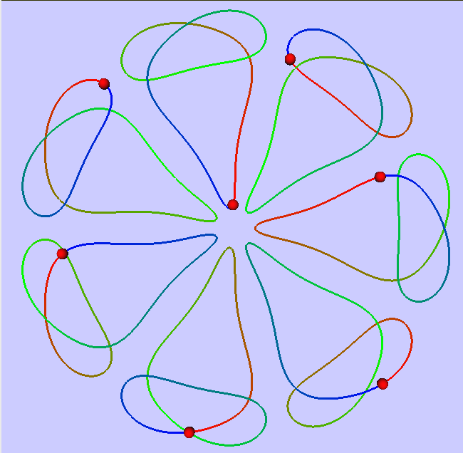
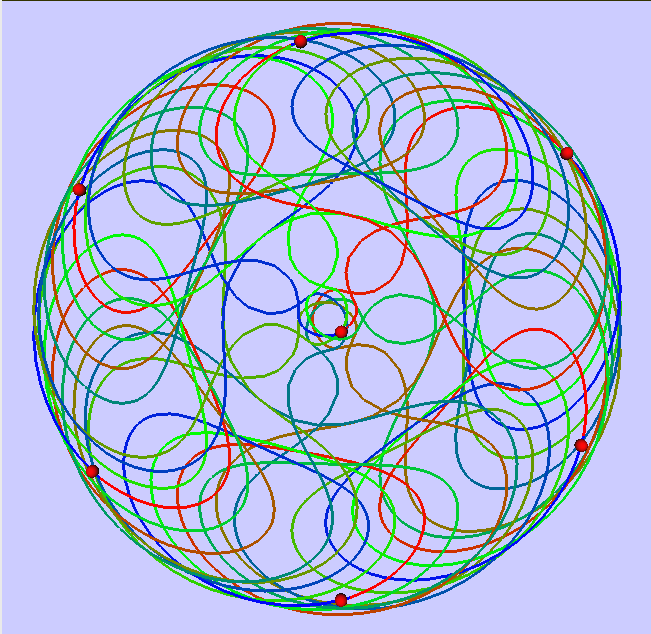
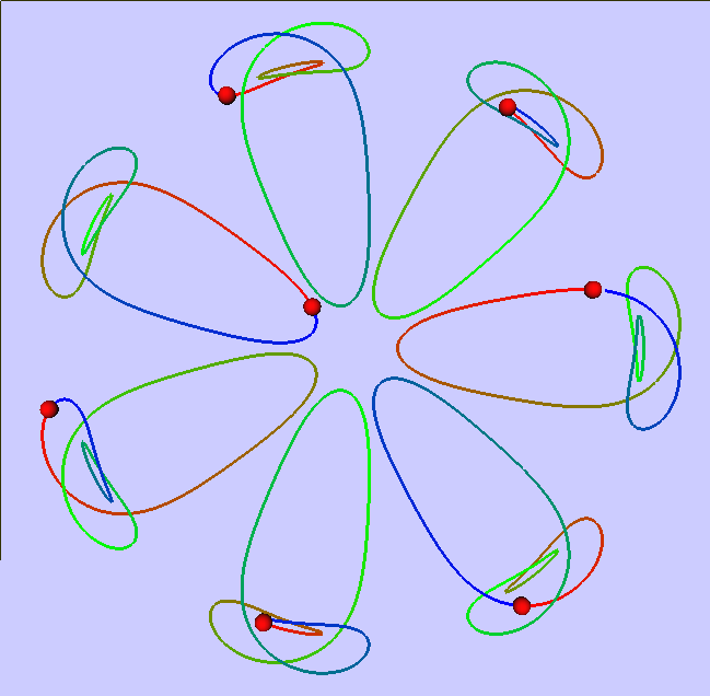
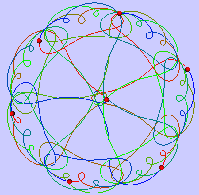
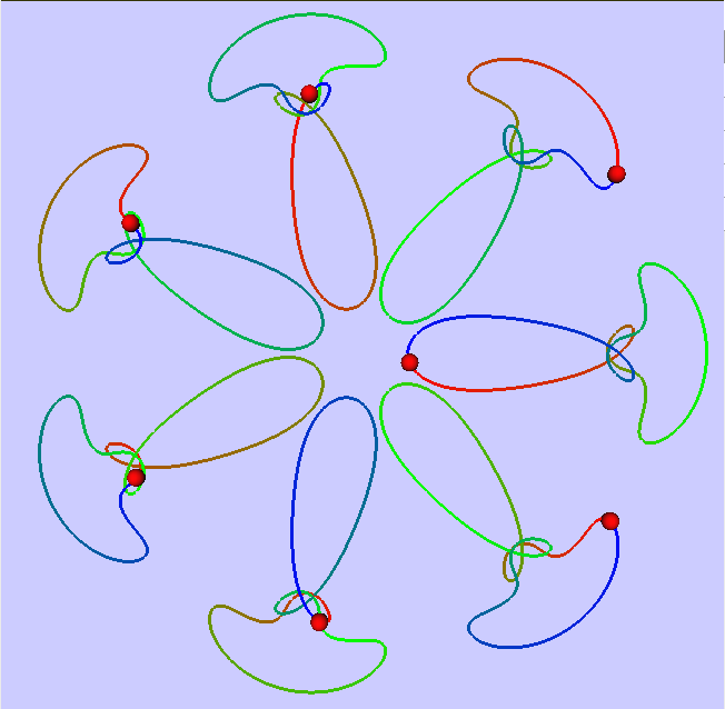
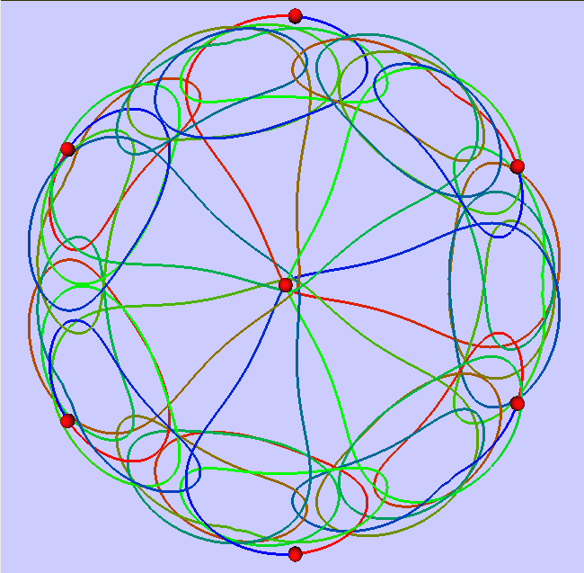
Figure 1: Some orbits along Planar families for the case $n=7$. Top: two orbits with $k=2$. Center: two orbits with $k=3$. Bottom: two orbits with $k=4$.

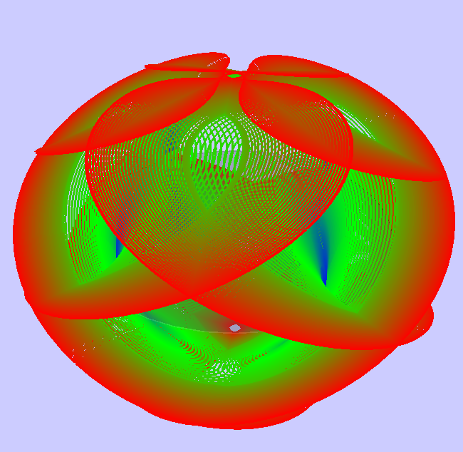
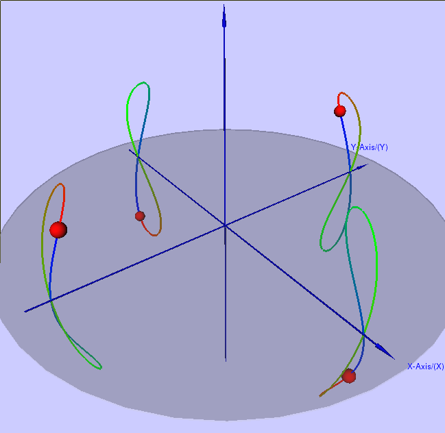
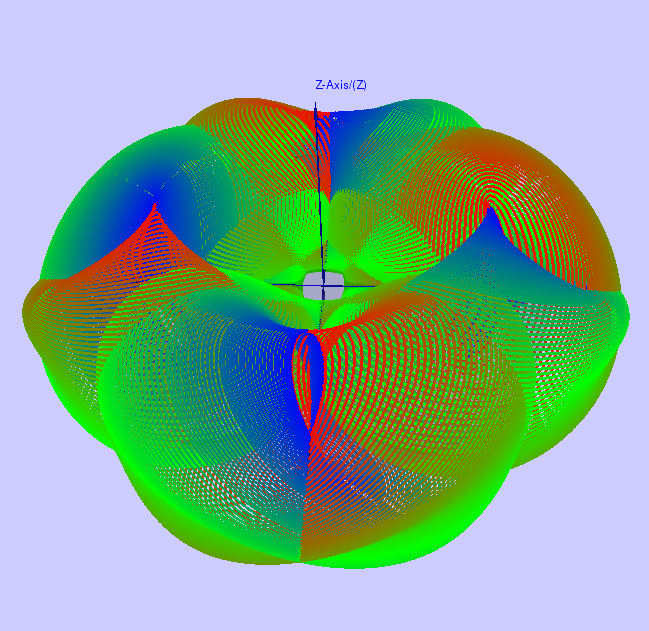
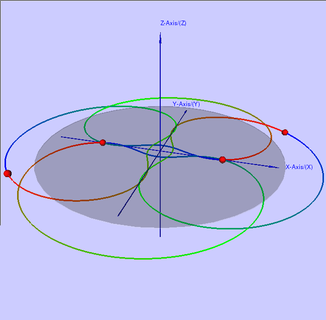
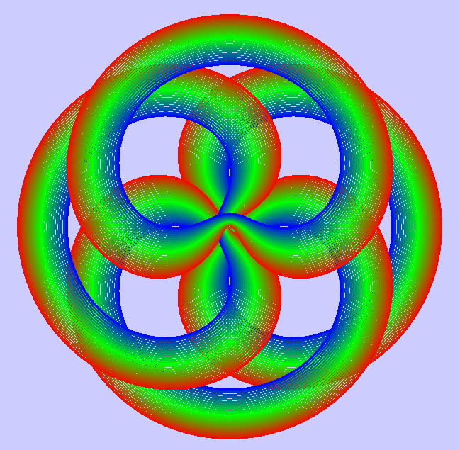
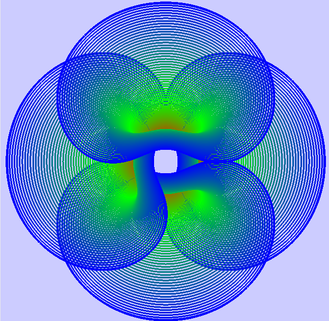
Figure 2: Top-Left: the Vertical Lyapunov family for $n=4$ and $k=2$. Top-Right: the first bifurcation orbit along the Vertical family. Center-Left: the Axial family that bifurcates from the Vertical family. Center-Right: the bifurcation orbit where the Axial family connects to to a Planar family. Bottom-Left: one branch of the Planar family to which the Axial family connects. Bottom-Right: the other branch of the family to which the Axial family connects.

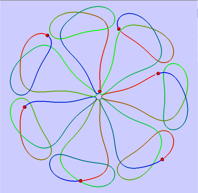
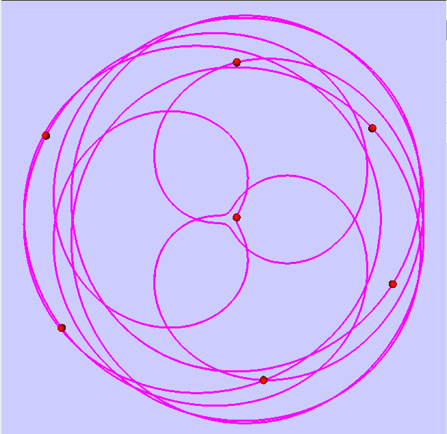
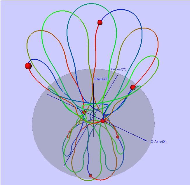
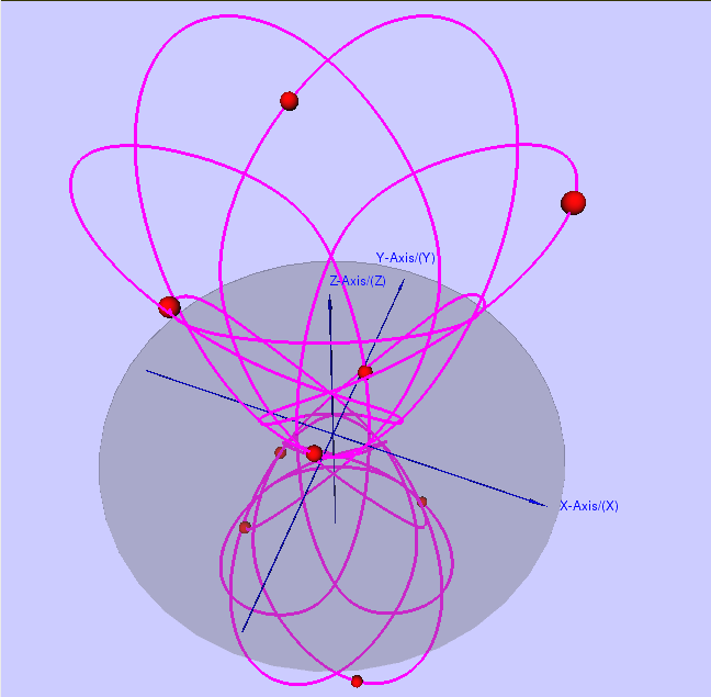
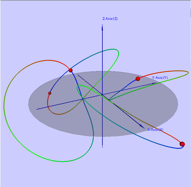
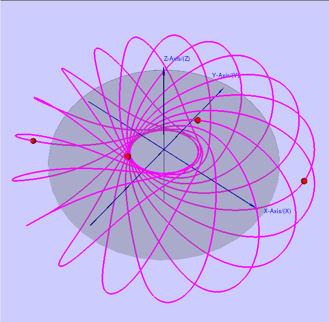
Figure 3: The panels on the left show orbits in the rotating frame, while the panels on the right show the same orbits in the inertial frame, where they correspond to choreographies. Top: a resonant Planar Lyapunov orbit. Center: a resonant Vertical Lyapunov orbit. Bottom: a resonant Axial orbit.

4 Choreographies along Planar Lyapunov families

In this section we present some of the infinitely many choreographies that appear along the Planar Lyapunov families, namely for the cases $n=7$, $n=8$ and $n=9$, as shown in Figures 4, 5, and 6, respectively. Corresponding data are given in Tables 1 - 3. Each choreography winds $\ell$ times around a center and is invariant under rotations of $2\pi/m$. The bodies move in groups of $d$-polygons, where $d$ is the greatest common divisor of $n$ and $k$. In addition these choreographies are symmetric with respect to reflection in the plane generated by the second symmetry in (4).

When there is an infinite number of choreographies then the winding number $\ell$ and the symmetry indicator $m$ can be arbitrarily large, and the choreography arbitrarily complex. From the observed range of values of the periods along a Lyapunov family we mostly choose the simpler resonances, and hence the simpler choreographies. For example, the family $k=2$ for $n=7$ has a relatively simple choreography. Here $\ell=5$ and $m=3$ are relatively prime, with

$$k\ell-m=2\times 5-3=7\in n\mathbb{Z}\text{.}$$

In this example $2\pi s_{1}^{-1/2}=4.1387$, and since $T_{5:3}=(2\pi s_{1}^{-1/2})(5/3)=\allowbreak 6.8978$ is within the range of periods of the Lyapunov family, it follows that the $5:3$ resonant Lyapunov orbit corresponds to a choreography in the inertial frame. This choreography is shown in the center-right panel of Figure 4. It has period $3T_{5:3}$, winding number $5$, and it is invariant under rotations of $2\pi/3$. Similar statements apply to other planar choreographies.

For $n=7$ there is a sequence of Planar Lyapunov families having $k=2,3,4,2$, respectively. The last of these families, with $k=2$, has orbits of rather small amplitude, and is not included in the families shown in Figure 4.

$$k$$ Eigenvalue Period Interval Resonant Orbit

2 1.53960 [4.0811, 28.328] 4:1 and 5:3

3 1.85058 [3.3953, 27.974] 3:2 and 5:1

4 1.50806 [4.1664, 28.499] 2:1 and 15:4

2 0.761477 [8.2513 ,8.3328] –

Table 1: Data for $n=7$ bodies.

For $n=8$ there is a sequence of Planar Lyapunov family having $k=2,3,4,5,2$, respectively. We have chosen one choreography from each one of these families, with an additional one for $k=5$, in Figure 5.

$$k$$ Eigenvalue Period Interval Resonant Orbit

2 1.94947 [3.2230, 14.836] 11:6

3 2.39714 [2.6211, 29.654] 11:9

4 2.41171 [2.6053, 7.4935] 5:4

5 1.91468 [3.2814, 29.122] 5:1 and 9:5

2 0.435437 [5.4804, 14.430] 5:2

Table 2: Data for $n=8$ bodies.

For $n=9$ there is a sequence of Planar Lyapunov families having $k=2,3,4,5,6,2$, respectively. In Figure 6 we have selected one choreography from each of these families.

$$k$$ Eigenvalue Period Interval Resonant Orbit

2 2.27175 [2.7660, 30] 5:1

3 2.85442 [2.2012, 10.298] 4:3

4 3.06012 [2.0534, 30.411] 5:2

5 2.90713 [2.1613, 30.612] 2:1

6 2.26399 [2.7197, 10.008] 5:3

2 0.196565 [15.400, 31.927] 5:1

Table 3: Data for $n=9$ bodies.

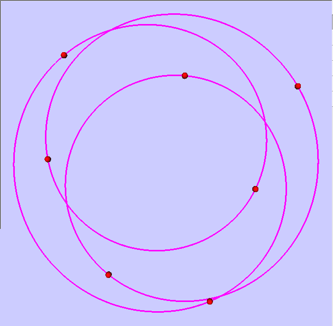
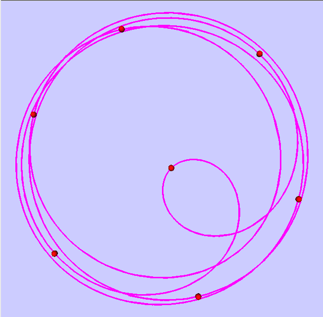
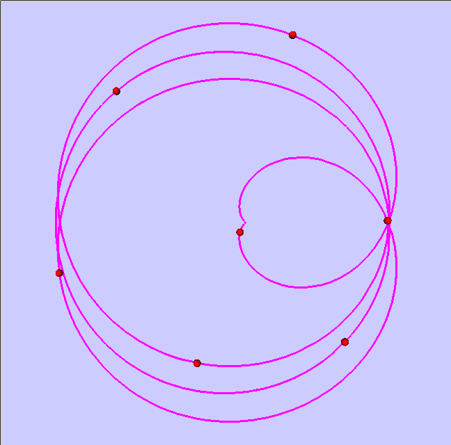
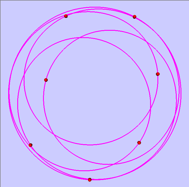
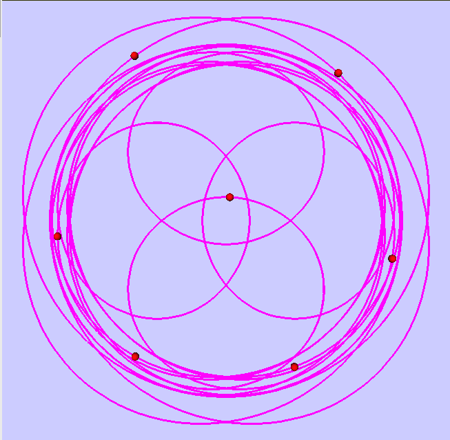
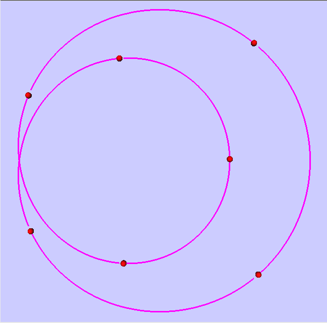
Figure 4: Planar choreographies for $n=7$ bodies: Top-Left: a $3:2$-resonant orbit for $k=3$. Top-Right: a $5:1$-resonant orbit for $k=3$. Center-Left: a $4:1$-resonant orbit for $k=2$. Center-Right: a $5:3$-resonant orbit for $k=2$. Bottom-Left: a $15:4$-resonant for orbit for $k=4$. Bottom-Right: a $2:1$-resonant orbit for $k=4$.

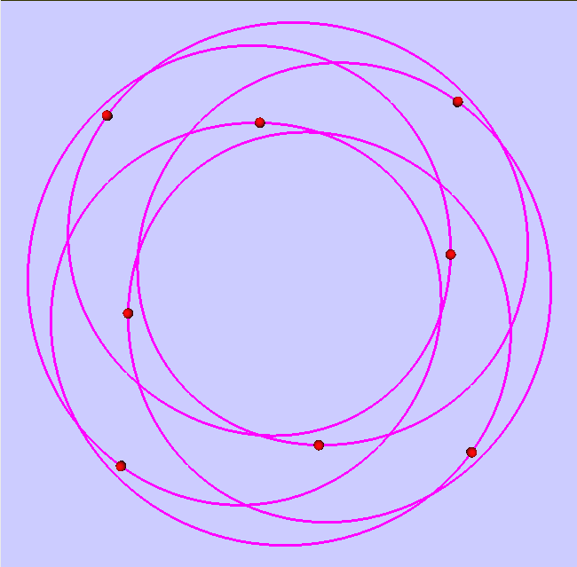
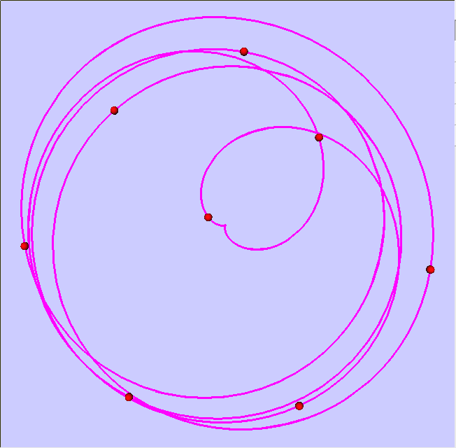
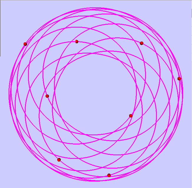
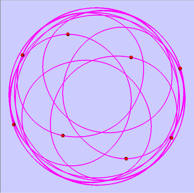
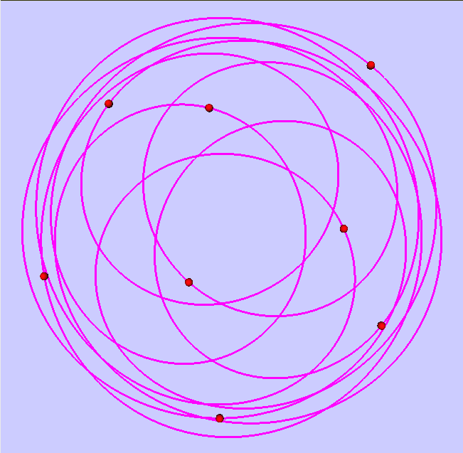
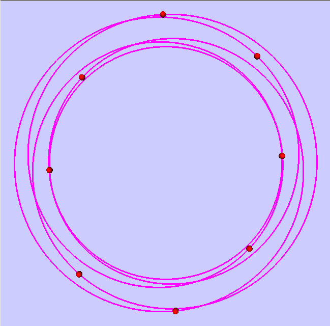
Figure 5: Planar choreographies for $n=8$. Top-Left: a $5:4$-resonant orbit for $k=4$. Top-Right: a $5:1$-resonant orbit for $k=5$. Center-Left: an $11:9$-resonant orbit for $k=3$. Center-Right: an $11:6$-resonant orbit for $k=2$. Bottom-Left: a $9:5$-resonant orbit for $k=5$. Bottom-Right: a $5:2$-resonant orbit for $k=2$.

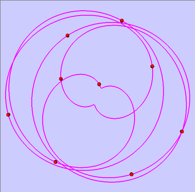
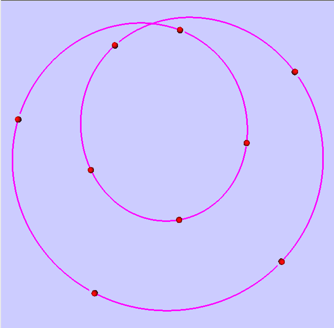
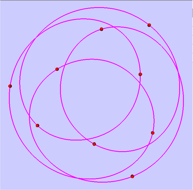
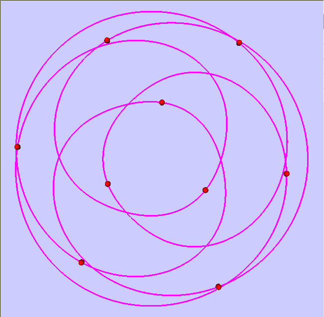
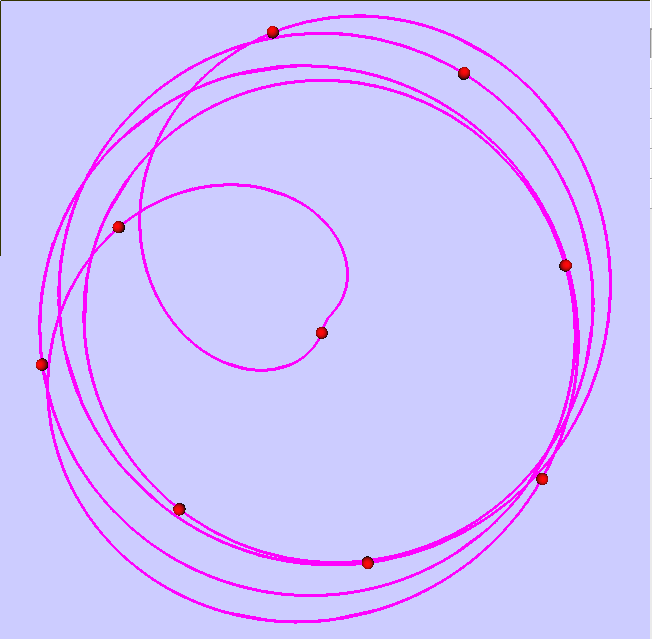
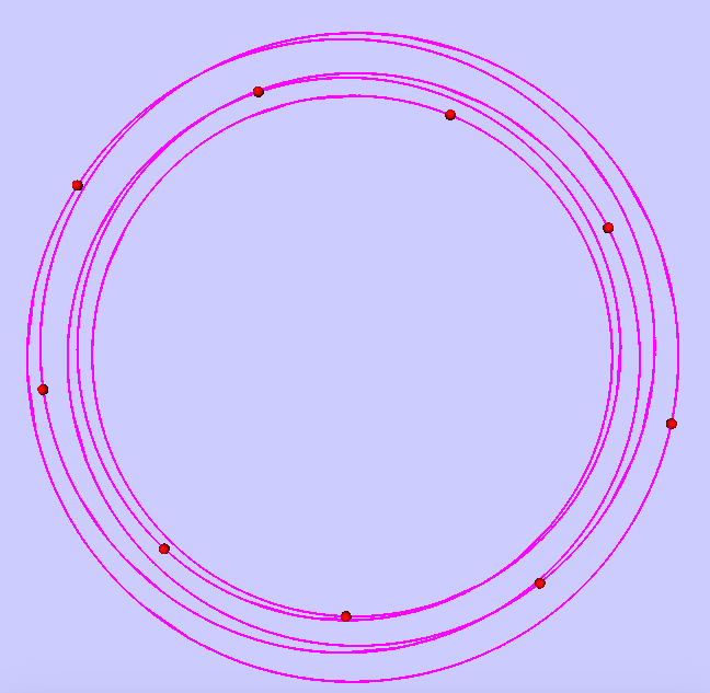
Figure 6: Planar choreographies for $n=9$. Top-Left: a $5:2$-resonant orbit for $k=4$. Top-Right: a $2:1$-resonant orbit for $k=5$. Center-Left: a $4:3$-resonant orbit for $k=3$. Center-Right: a $5:3$-resonant orbit for $k=6$. Bottom-Left: a $5:1$-resonant orbit for $k=2$. Bottom-Right: a $5:1$-resonant orbit for $k=2$.

5 Choreographies along Vertical Lyapunov families and their bifurcating families

In this section we give examples of choreographies along the Vertical Lyapunov families and along their bifurcating families. The projections of these choreographies onto the $xy$-plane are invariant under rotations of $2\pi/m$. The bodies form groups of $d$-polygons, where $d$ is the greatest common divisor of $n$ and $k$. Since we obtain choreographies by rotating closed orbits, each choreography is contained in a surface of revolution. Indeed, due to the symmetries of the Vertical families the choreographies wind around a cylindrical manifold with winding number $\ell$, while for the Axial families the choreographies wind around a toroidal manifold with winding numbers $\ell$ and $m$.

The spatial choreographies along the Vertical Lyapunov families are symmetric with respect to the reflections $-y$ and $-z$, when the $x$-axis is chosen to pass through the “center”of the orbit. While planar choreographies for large values of $\ell$ and $m$ are somewhat difficult to appreciate, spatial choreographies of this type are easier to visualize because they wind around a cylindrical manifold. For even values of $n$ we mention the case $k=n/2$, for which the orbits of the Vertical family are known as Hip-Hop orbits. Choreographies along such families have been described before in [28], and in [4], where they were found numerically as local minimizers of the action restricted to symmetric paths. Along Hip-Hop families we have located the choreography for $n=4$ found in [28]. Several choreographies along Hip-Hop families are shown the top four panels of Figure 7. We have not computed all Vertical families, due to presence of double resonant eigenvalues. For the case $n=9$, we show two choreographies along a family of periodic orbits that is not a Hip-Hop family, namely in the two bottom panels of Figure 7. Such families were not determined in [4] because they do not correspond to local minimizers of the action. Further investigation is needed for a systematic approach to determine these families.

We now present some choreographies along the families that emanate from the first bifurcation along Hip-Hop families in the rotating frame. The projections of these spatial choreographies onto the $xy$-plane are somewhat similar to those along the Planar Lyapunov orbits. However, the spatial periodic orbits in the rotating frame that correspond to these choreographies have only one symmetry, which is given by the transformation $(-y,-z)$ when the $x$-axis is chosen to pass through the “center”of the orbit in the rotating frame; see the bottom left panel of Figure 3. This is due to the fact that the Axial family arises from the Vertical Lyapunov family via a symmetry-breaking bifurcation. The symmetry implies that choreographies along the Axial families wind around a toroidal manifold with winding numbers $\ell$ and $m$. Since we assume that $\ell$ and $m$ are co-prime, the choreography path is known as a torus knot. The simplest nontrivial example is the $(2,3)$-torus knot, also known as the trefoil knot. We note that for other integers $\ell$ and $m$ such that $k\ell-m\notin n\mathbb{Z}$, the orbit of the $n$ bodies in the inertial frame consists of separate curves that form a torus link. Some of the choreographies along the Axial families are shown in Figure 8.

In Section 3 we already mentioned that there are planar bifurcation orbits along Axial families that give rise to planar families. Such an Axial family and its planar bifurcation orbit are shown in the center panels of Figure 2, namely for the case $n=4$. Orbits along the two branches of the bifurcating planar family are shown in the bottom panels. Specifically, our numerical computations indicate that Hip-Hop families connect indirectly to planar families via the above-described tertiary bifurcation. Choreographies along such planar families have symmetries that are similar to those of Planar Lyapunov families, although in fact these families do not correspond to Lyapunov families. While there are no Planar Lyapunov families for $n=4,5$, and $6$, there are such tertiary planar families for these values of $n$, and these contain planar choreographies. Such choreographies are called unchained polygons in [4], and there are infinitely many of these. In particular, the Vertical family for $n=3$ and $k=1$ leads indirectly to the planar $P_{12}$-family of Marchal [20]. We have continued such families numerically for $k=n/2$, where $n=4,6$, and $8$, and six choreographies along them are shown in the panels of Figure 9.

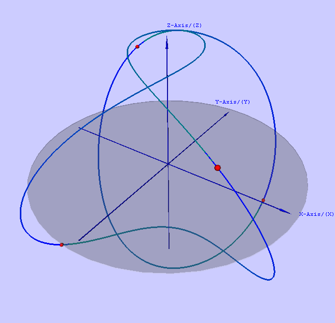
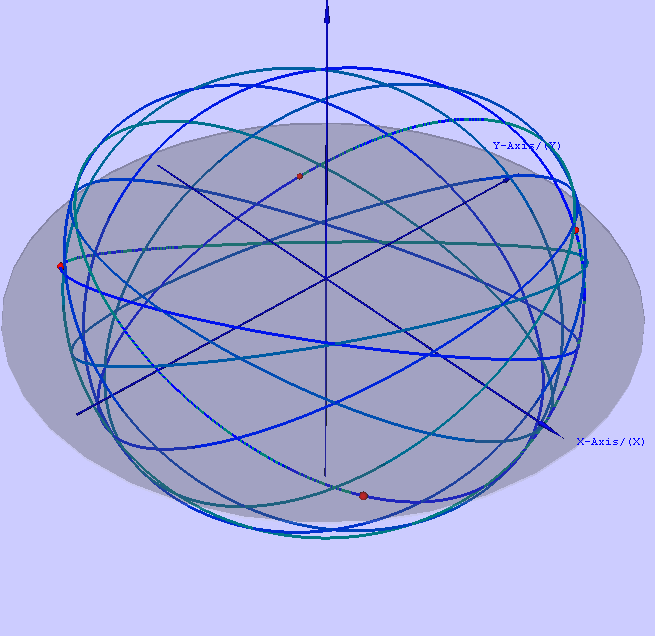
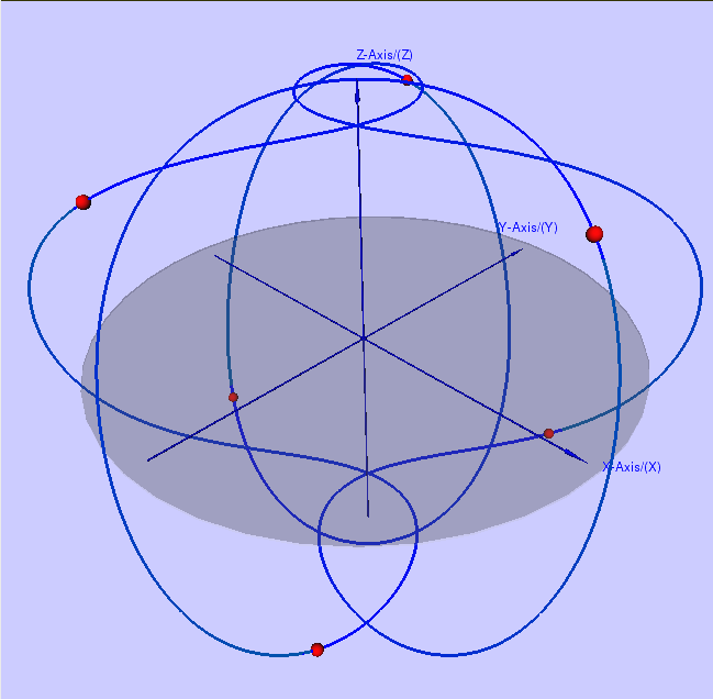
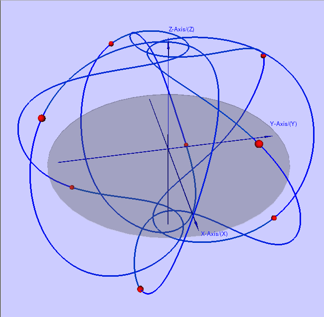
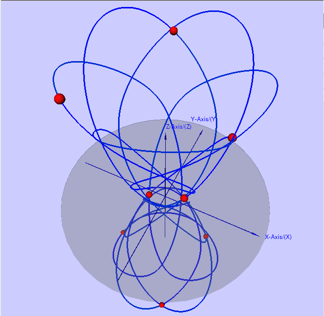
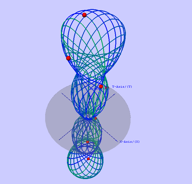
Figure 7: Vertical Lyapunov families. Top-Left: a $3:2$-resonant Hip-Hop orbit along $V_{1}$ for $n=4$. Top-Right: a $9:10$-resonant Hip-Hop orbit along $V_{1}$ for $n=4$. Center-Left: a $5:3$-resonant Hip-Hop along $V_{1}$ for $n=6$. Center-Right: a $7:4$-resonant Hip-Hop along $V_{1}$ for $n=8$. Bottom-Left: an $11:5$ resonance along $V_{3}$ for $n=9$. Bottom-Right: a $17:5$ resonance along $V_{3}$ for $n=9$.

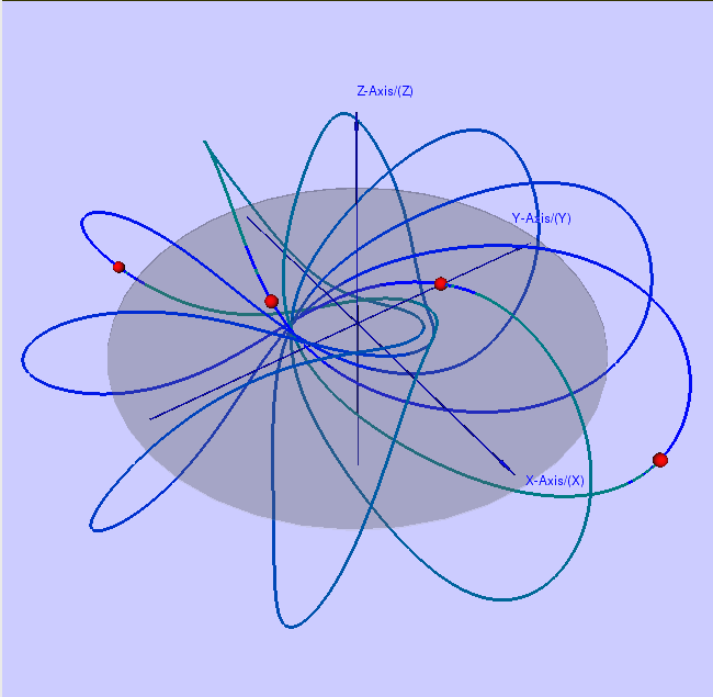
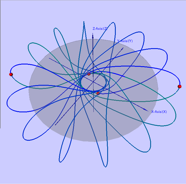
Figure 8: Resonant Axial orbits with $k=n/2$. Top-Left: a $7:10$ resonant Axial orbit for $n=4$. Top-Right: a $9:14$ resonant Axial orbit for $n=4$. Center-Left: a $5:9$ resonant Axial orbit for $n=6$. Center-Right: an $11:15$ resonant Axial orbit for $n=6$. Bottom-Left: a $7:12$ resonant orbit for $n=8$. Bottom-Right: a $15:28$ resonant Axial orbit for $n=8$.

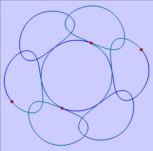
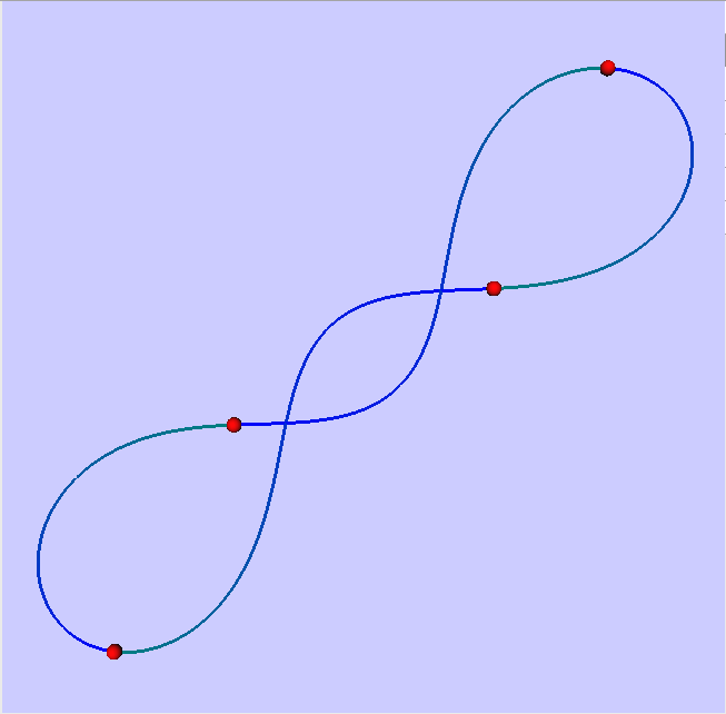
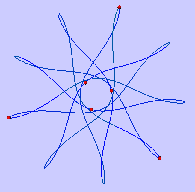
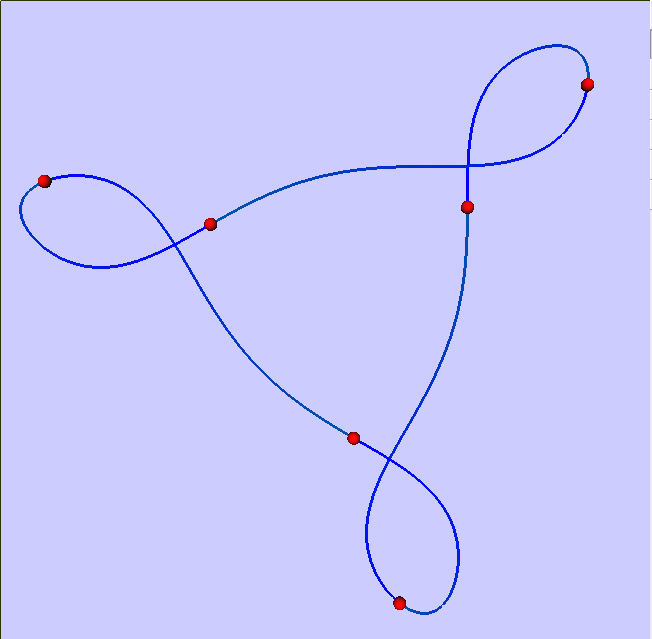
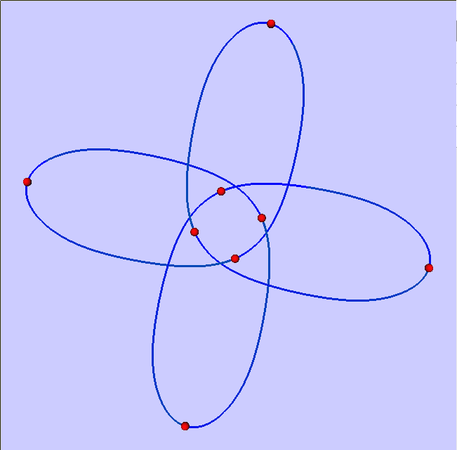
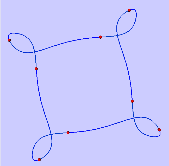
Figure 9: Unchained polygons for $k=n/2$. Top-Left: a $1:6$ resonant orbit for $n=4$. Top-Right: a $1:2$ resonant orbit for $n=4$. Center-Left: a $5:9$ resonant orbit for $n=6$. Center-Right: a $1:3$ resonant orbit for $n=6$. Bottom-Left: a $3:4$ resonant orbit for $n=8$. Bottom-Right: a $1:4$ resonant orbit for $n=8$.

6 Other configurations

6.1 The Maxwell configuration

The choreographies in the preceding sections are unstable, in part because they arise directly or indirectly from an unstable relative equilibrium. To determine stable solutions it is helpful to consider orbits that emanate from a stable relative equilibrium. The polygonal equilibrium is never stable; about half of its eigenvalues are stable and about half are unstable. For this reason we now consider the Maxwell configuration, consisting of an $n$-polygon with an additional massive body at the center, which is known to be stable when $n\geq 7$. Specifically, the central body has mass $m_{0}=\mu$, and the other $n$ bodies have equal mass $m_{j}=1$ for $j\in\{1,...,n\}$. Let $(u_{j},z_{j})\in\mathbb{C}\times\mathbb{R}$ be the position of body $j\in\{0,1,...,n\}$. The Newton equations of motion for the $n+1$ bodies in rotating coordinates

$$q_{j}(t)=(e^{i\sqrt{\omega}t}u_{j}(t),z_{j}(t))$$

have an equilibrium with $\left(u_{0},z_{0}\right)=\left(0,0\right)$ and $\left(u_{j},z_{j}\right)=\left(e^{ij\zeta},0\right)$ for $j\in\{1,...,n\}$, where $\zeta=2\pi/n$ and

$$\omega=\mu+s_{1}\text{.}$$

This well-known Maxwell configuration reduces to the polygonal relative equilibrium when $\mu=0$.

For $n\geq 7$ all planar eigenvalues are imaginary, and produce Planar Lyapunov families. The $n+1$ spatial eigenvalues include $0$ (due to symmetries), $i\sqrt{\mu+n}$ for $k=n$, and

$$i\sqrt{\mu+s_{k}},\qquad k=1,~{}\cdots~{},n-1\text{.}$$

The frequency $\sqrt{\mu+n}$ produces the Vertical Lyapunov family, which corresponds to the oscillatory ring in [22]. For $k=n/2$, with $n$ even, we obtain a Hip-Hop family [22]. For the Maxwell configuration we say that a Lyapunov orbit is $\ell:m$ resonant when its period satisfies

$$T_{\ell:m}=\frac{2\pi}{\sqrt{\mu+s_{1}}}\frac{\ell}{m},$$

where $\ell$ and $m$ are relatively prime such that $k\ell-m\in n\mathbb{Z}$. For an $\ell:m$ resonant Lyapunov orbit the $n$ bodies of equal mass follow the same path as in Theorem 5.

To illustrate our numerical computations we chose the first stable case for $\mu=200$, namely $n=7$. We also consider the case $n=8$ with $\mu=300$. We computed many families for $n=7$ and $n=8$ and we present only a few planar resonant orbits in Figure 11 and spatial resonant orbits in Figure 12.

6.2 A triangular configuration

Here we present some families of periodic solutions that emanate from the “triangular” equilibrium shown in the top-left panel of Figure 12, with $9$ bodies of equal mass. Periodic solutions that emanate from the triangular equilibrium have been determined with the same numerical scheme used throughout this paper. However, a detailed description of these results is outside the scope of the current paper, whose aim is the continuation of solutions with symmetries that produce choreographies.

The triangular equilibrium can been reached by following one of the families of spatial periodic orbits that bifurcate from the polygonal relative equilibrium for $n=9$. These spatial solutions have the symmetry

$$u_{j}(t)=\bar{u}_{n-j}(-t)\text{.}$$

Actually, in addition to the Vertical Lyapunov families that produce choreographies from the polygonal configuration, we have also determined these solutions, which do not produce choreographies. To the best of our knowledge, the existence of these families has not been established before.

Acknowledgements. We would like to thank R. Montgomery, J. Montaldi, D. Ayala and L. García-Naranjo for many interesting discussions. We also acknowledge the assistance of Ramiro Chavez Tovar with the preparation of figures and animations.

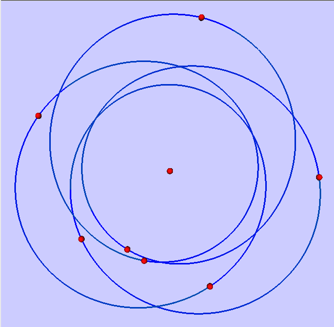
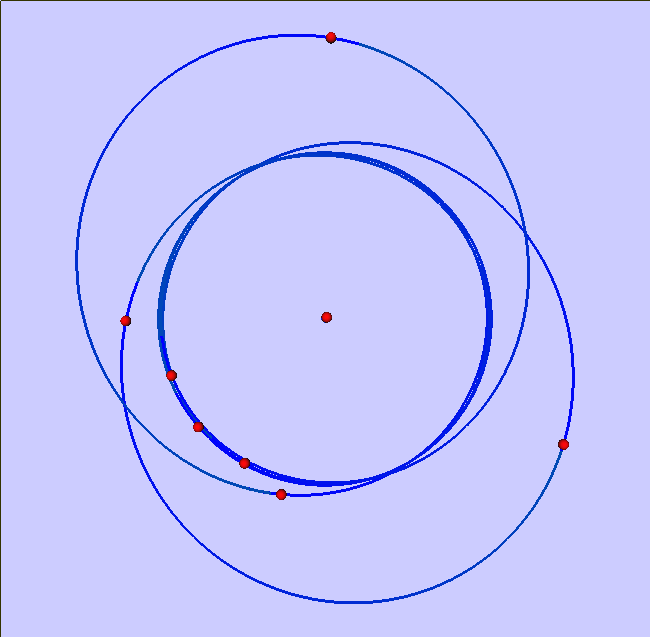
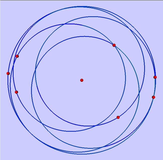
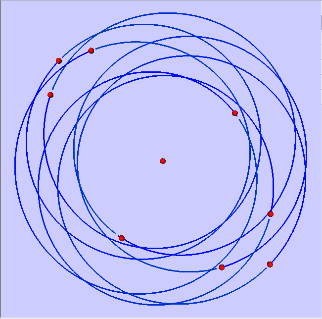
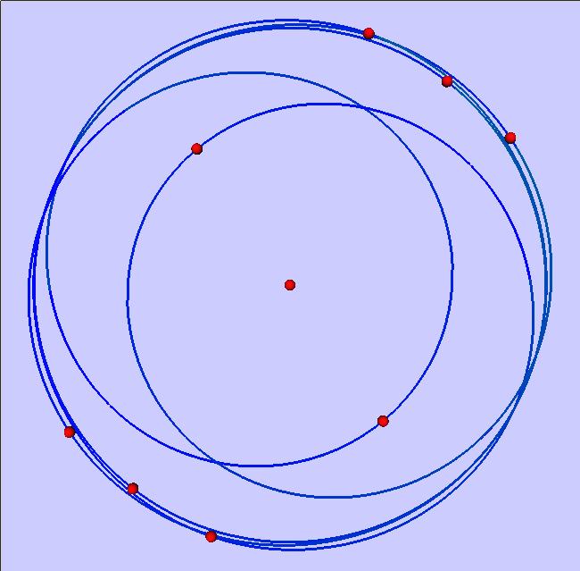
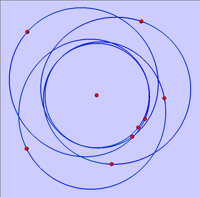
Figure 10: Top-Left: a $4:3$ resonant orbit for $7+1$ bodies and $k=6$. Top-Right: a $5:2$ resonant orbit for $7+1$ bodies and $k=6$. Center-Left: a $5:3$ resonant orbit for $7+1$ bodies and $k=2$. Center-Right: a $7:3$ resonant orbit for $8+1$ bodies for $k=8$. Bottom-Left: a $5:2$ resonant orbit for $8+1$ bodies and $k=2$. Bottom-Right: a $5:3$ resonant orbit for $8+1$ bodies and $k=7$.

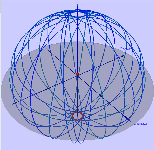
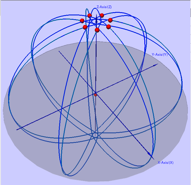
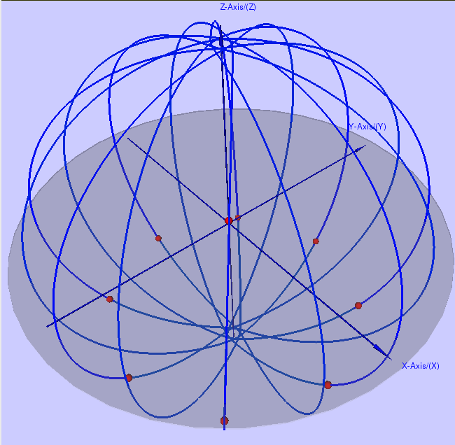
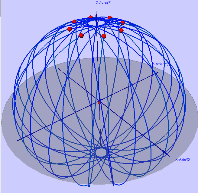
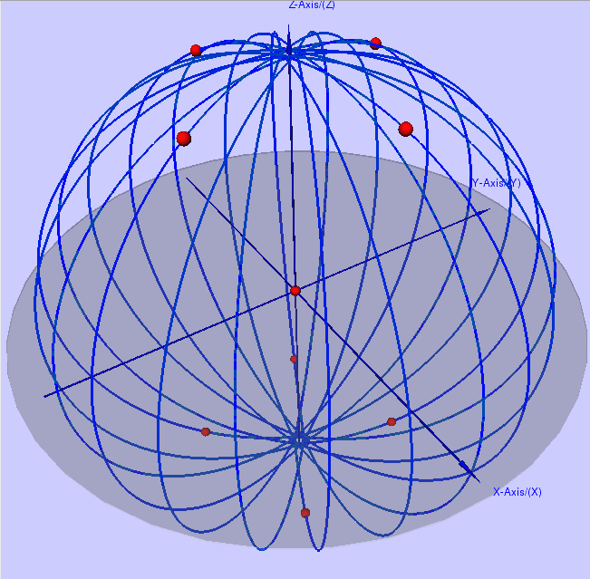
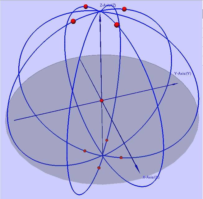
Figure 11: Top-Left: a $15:14$ resonant orbit for $7+1$ bodies and $k=7$. Top-Right: an $8:7$ resonant orbit for $7+1$ bodies and $k=7$. Center-Left: a $9:8$ resonant orbit for $8+1$ bodies and $k=8$. Center-Right:a $17:16$ resonant orbit for $8+1$ bodies and $k=8$. Bottom-Left: a $13:12$ resonant orbit for $8+1$ bodies and $k=4$. Bottom-Right: a $15:12$ resonant orbit for $8+1$ bodies and $k=4$.

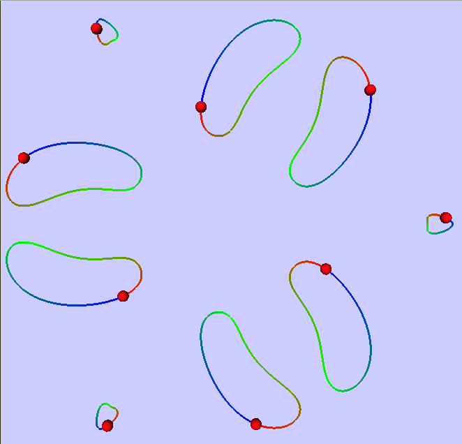
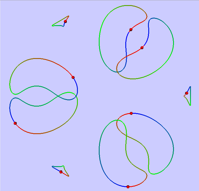
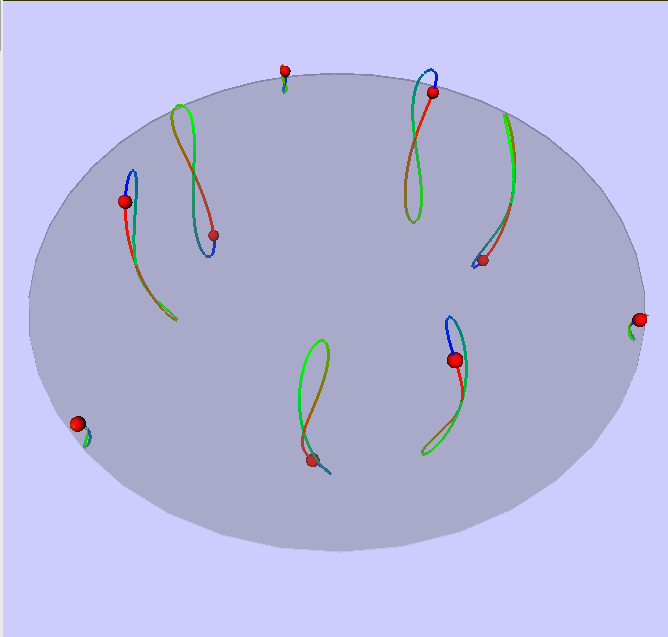
Figure 12: Some Lyapunov families with different symmetries for $n=9$. Top-Left: another equilibrium of the 9-body problem. Top-Right: an orbit along a bifurcating Planar family. Center-Left: an orbit along another bifurcating Planar family. Center-Right: an orbit along yet another bifurcating Planar family. Bottom-Left: an orbit along a bifurcating spatial family. Bottom-Right: an orbit along another bifurcating spatial family.

References

- [1] E. Barrabés, J. M. Cors, C. Pinyol, and J. Soler. Hip-hop solutions of the -body problem. Celestial Mech. Dynam. Astronom., 95(1-4):55–66, 2006.
- [2] V. Barutello, D. Ferrario , S. Terracini. Symmetry groups of the planar 3-body problem and action-mimizing trajectories. Archive for Rational Mechanics and Analysis 190 (2008), 189–226.
- [3] K.-C. Chen. Binary Decompositions for Planar N-Body Problems and Symmetric Periodic Solutions. Arch. Ration. Mech. Anal. 170: 247–276, 2003.
- [4] A. Chenciner and J. Fejoz. Unchained polygons and the -body problem. Regular and chaotic dynamics, 14, (1): 64–115, 2009.
- [5] A. Chenciner, J. Féjoz J. and R. Montgomery, (2005), Rotating Eights I: the three families. Nonlinearity 18 1407-1424.
- [6] A. Chenciner, J. Gerver, R. Montgomery, C. Simó, Simple Choreographic Motions of N bodies. A preliminary study, in Geometry, Mechanics, and Dynamics, 60th birthday of J.E. Marsden. P. Newton, P. Holmes, A. Weinstein, ed., Springer-Verlag, 2002.
- [7] A. Chenciner and R. Montgomery.A remarkable periodic solution of the three-body problem in the case of equal masses. Ann. of Math. 152, (2), 881–901, 2000.
- [8] I. Davies, A. Truman, and D. Williams. Classical periodic solutions of the equal-mass -body problem, -ion problem and the -electron atom problem. Physics Letters A., 99(1):15–18, 1983.
- [9] E. Doedel, E. Freire , J. Galán, F. Muñoz-Almaraz, A. Vanderbauwhede. Stability and bifurcations of the figure-8 solution of the three-body problem. Phys Rev Lett. 88 (2002) 241101.
- [10] E. Doedel, E. Freire , J. Galán, F. Muñoz-Almaraz, A. Vanderbauwhede. Continuation of periodic orbits in conservative and Hamiltonian systems. Physica D: Nonlinear Phenomena 181 (2003) 1-38
- [11] D. Ferrario. Symmetry groups and non-planar collisionless action-minimizing solutions of the three-body problem in three-dimensional space. Arch. Ration. Mech. Anal. 179: (3), 389–412, 2006.
- [12] D. Ferrario and A. Portaluri. On the dihedral -body problem. Nonlinearity 21: (6), 1307–1321, 2008.
- [13] D. Ferrario and S. Terracini. On the existence of collisionless equivariant minimizers for the classical -body problem. Invent. Math. 155:(2), 305–362, 2004.
- [14] C. García-Azpeitia, J. Ize. Global bifurcation of polygonal relative equilibria for masses, vortices and dNLS oscillators. J. Differential Equations 251 (2011) 3202–3227.
- [15] C. García-Azpeitia, J. Ize. Global bifurcation of planar and spatial periodic solutions from the polygonal relative equilibria for the -body problem. J. Differential Equations 254 (2013) 2033–2075.
- [16] J. Ize and A. Vignoli. Equivariant degree theory. De Gruyter Series in Nonlinear Analysis and Applications 8. Walter de Gruyter, Berlin, 2003.
- [17] T. Kapela, P. Zgliczynski. An existence of simple choreographies for N-body problem – a computer assisted proof. Nonlinearity 16 (2003) 1899-1918
- [18] T. Kapela, C. Simó. Computer assisted proofs for nonsymmetric planar choreographies and for stability of the Eight. Nonlinearity (2007), 20, 1241-1255.
- [19] T. Kapela, C. Simó. Rigorous KAM results around arbitrary periodic orbits for Hamiltonian Systems, Preprint.
- [20] C. Marchal. The family P12 of the three-body problem. The simplest family of periodic orbits with twelve symmetries per period. Celestial Mechanics and Dynamical Astronomy 78 (2000) 279–298
- [21] C. Marchal. How the method of minimization of action avoids singularities. Celestial Mech. Dynam. Astronom. 83 (2002) 325–353.
- [22] K. Meyer and D. Schmidt. Librations of central configurations and braided saturn rings. Celestial Mech. Dynam. Astronom. 55(3):289–303, 1993.
- [23] R. Moeckel. Linear stability of relative equilibria with a dominant mass. J. of Dynamics and Differential Equations, 6:37–51, 1994.
- [24] C. Moore. Braids in Classical Gravity. Physical Review Letters 70 (1993) 3675–3679.
- [25] J. Montaldi, K. Steckles. Classification of symmetry groups for planar n-body choreographies. Forum of Mathematics, Sigma. 1 (2013).
- [26] G. E. Roberts. Linear stability in the -gon relative equilibrium. In J. Delgado, editor, Hamiltonian systems and celestial mechanics. HAMSYS-98. Proceedings of the 3rd international symposium, World Sci. Monogr. Ser. Math. 6, pages 303–330. World Scientific, 2000.
- [27] C. Simó. New Families of Solutions in N-Body Problems. European Congress of Mathematics 101–115. Springer Nature, 2001.
- [28] S. Terracini and A. Venturelli. Symmetric trajectories for the -body problem with equal masses. Arch. Rat. Mech. Anal. , 184(3):465–493, 2007.
- [29] R.J Vanderbei and E. Kolemen. Linear stability of ring systems. The astronomical journal 133: 656–664, 2007.