Electric current filamentation induced by 3D plasma flows in the solar corona

Abstract

Many magnetic structures in the solar atmosphere evolve rather slowly so that they can be assumed as (quasi-)static or (quasi-)stationary and represented via magneto-hydrostatic (MHS) or stationary magneto-hydrodynamic (MHD) equilibria, respectively. While exact 3D solutions would be desired, they are extremely difficult to find in stationary MHD. We construct solutions with magnetic and flow vector fields that have three components depending on all three coordinates. We show that the non-canonical transformation method produces quasi-3D solutions of stationary MHD by mapping 2D or 2.5D MHS equilibria to corresponding stationary-MHD states, i.e., states that display the same field line structure as the original MHS equilibria. These stationary-MHD states exist on magnetic flux surfaces of the original 2D MHS-states. Although the flux surfaces and therefore also the equilibria have a 2D character, these stationary MHD-states depend on all three coordinates and display highly complex currents. The existence of geometrically complex 3D currents within symmetric field-line structures provide the base for efficient dissipation of the magnetic energy in the solar corona by Ohmic heating. We also discuss the possibility of maintaining an important subset of non-linear MHS states, namely force-free fields, by stationary flows. We find that force-free fields with non-linear flows only arise under severe restrictions of the field-line geometry and of the magnetic flux density distribution.

1 Introduction

Many structures in the atmosphere of the sun and in solar-type stars evolve on relatively large time-scales so that they can be described within the frame of quasi-stationary or quasi-static magneto-hydrodynamics (MHD). Prominent examples are solar arcade structures, loops as well as prominences. For their representation typically magneto-hydrostatic (MHS) equilibria (e.g., Low, 1982; Solov’ev & Kirichek, 2015) or stationary-state models, i.e., stationary MHD equilibria, are calculated (e.g., Petrie & Neukirch, 1999; Petrie et al., 2005).

Generally, it would be desirable to have a full 3D representation of the MHD equilibrium states. However, as was already mentioned by Parker (1972), it is normally not possible to construct 3D states in the functional vicinity of 2D states. This means that 2D equilibria on which perturbations are imposed typically do not relax into smooth 3D states (Tsinganos, 1982). Instead, the resulting equilibria must contain tangential discontinuities, i.e., singular currrent sheets. This is known as Parker’s conjecture (Parker, 1983a, b, 1988) which states that no regular equilibria exist without a symmetry. In this context, symmetry does not necessarily imply that the system has an ignorable coordinate (Low, 1985), where ignorable coordinate means that in a specific coordinate system the physical values do not depend on this coordinate. We note that under specific circumstances a few regular classes of 3D MHS states have been found (see, e.g., Low, 1982; Neukirch, 1995), and a set of exact analytical 3D stationary MHD flows exists as well (see, e.g., Bogoyavlenskij, 2001, 2002), however, the computation of these solutions requires that a complete stationary flow must already be known.

According to Parker, the appearance of singular current sheets could provide a suitable mechanism for acceleration and heating of the coronal plasma via Ohmic heating, i.e., Joule dissipation, caused by magnetic reconnection within these current sheets. To guarantee that heating is provided on a regular base (i.e. also during times with no huge eruptions), successive heating should take place. This can only be achieved considering quasi-continuous small scale eruptions, the so-called nanoflares (Parker, 1988). However, it is still highly debated whether large-scale eruptions or small-scale nanoflares are the major mechanism for the heating of the solar coronal plasma (see, e.g., Parnell & De Moortel, 2012; Švanda & Karlický, 2016).

Shearing motions of the magnetic field lines, e.g. at the footpoints of arcade structures, can be used to produce nanoflares (see, e.g., Bingert & Peter, 2011; Bourdin et al., 2013; Hansteen et al., 2015) or large-scale eruptions (e.g., Manchester, 2003; Kotrč et al., 2013; Toriumi et al., 2013; Leake et al., 2014). Such a procedure does not necessarily converge into an equilibrium state anymore. Therefore, in numerical simulations these sheared field lines might be forced to relax into an equilibrium state by introducing numerical resistivities and viscosities (e.g., Wilmot-Smith et al., 2011; Prior & Yeates, 2016).

Another approach for small-scale eruptions and heating was made by Pongkitiwanichakul et al. (2015), who applied a so-called volumetric Parker model. This model is not based on the shearing motions of the footpoints. Instead, a large-scale motion of the magnetic field lines is applied throughout the volume of the fluid. This large-scale motion is driven by an initial stationary flow, generated by a time-dependent stream function whose Fourier components are kept fixed at each time step. These stationary flows generate additional turbulent flows, which are allowed to evolve in time.

Alternatively, a model including selfconsistent plasma flows was developed by Nickeler et al. (2013, 2014). This model produces highly fragmented, strongly peaked currents and vortices spreading from large to small scales, while the system remains in a well-defined equilibrium.

In most of the aforementioned approaches, the initial condition is either a static or some arbitrary field that is non compatible with the resulting flow field. The numerically calculated corresponding changes of the fields are, therefore, based either on linear or non-linear perturbation theory or on stochastics. What is often neglected is that observations imply stationary flows in active regions and coronal holes rather than pure force-free or static fields (Winebarger et al., 2001, 2002; Marsch et al., 2004; Wiegelmann et al., 2005). Also, during pre-flare stages upflows in the photosphere and flows along loops were observed (e.g., Yoshimura et al., 1971; Harvey & Harvey, 1976; Wallace et al., 2010). Hence, an initial condition including stationary flows, as was presented by Nickeler & Wiegelmann (2010, 2012) seems more appropriate.

Non-linear MHD flow models for loops, sun spots, and magnetic arcade structures exist (see, e.g., Tsinganos et al., 1993; Petrie & Neukirch, 1999; Petrie et al., 2002, 2005), however, they were not developed explicitly for the purpose of explaining coronal heating. Nevertheless, non-linear MHD theory provides the proper tool for particle acceleration via generation of electric fields in a slightly non-ideal/resistive environment, and, therefore, for local heating processes (Nickeler et al., 2014).

In this paper, we wish to reinforce Parker’s conjecture of heating via multiple current sheets and multiple reconnection sites. In connection with the equilibrium problem introduced by Parker (1972) we need therefore a proper method that allows slight deviations from symmetric 2D to (almost) 3D structures. The known magnetic flux densities and the corresponding derived currents obtained from observations are far below the threshold for sufficient dissipation of magnetic energy in general, i.e. Joule heating by extremely strong currents in the case of e.g. Spitzer resistivity, and/or the threshold for anomalous resistivity triggering magnetic reconnection. This implies that the current density on these scales is too low to produce current-driven micro-instabilities. However, the observed large-scale fields might display steep gradients on smaller scales. Complex flow patterns and steep gradients in active regions indicate the existence of shear flows, as was reported by Marsch et al. (2004). The changing of the magnetic field structure often seems to coincide with sharp changes in the flows. Hence, this trend might be expected to continue when going to even smaller, yet unresolved scales.

For a better comprehension of Ohmic heating and acceleration of plasma and particles, we need more detailed information about current sheet structures in the solar atmosphere. While both observations and numerical simulations currently cannot resolve small-scale structures, an analytical approach is a useful physical approximation that provides detailed information down to the theoretical dissipation scales, which are for solar corona conditions below 10 m. Based on the non-canonical transformation method developed by Gebhardt & Kiessling (1992) and utilized by e.g. Cicogna & Pegoraro (2015), we will show that there is a connection between the breaking of the symmetry and the down-cascading of the current sheet scales. The breaking of the symmetry is done by field-aligned flows which have a strong gradient perpendicular to the field lines. These flows cause strong strong gradients of the magnetic field strength normal to the field lines, implying small-scale current sheets.

2 Problem description and basic assumptions

The magnetic field structures in the solar atmosphere, especially in the corona, resemble magnetic arches and also closed field line structures emulating flux ropes, surrounded by bundles of open field lines. These magnetic structures form the stage on which chromospheric and coronal heating takes place. For a reasonable representation of these structures, it is necessary to calculate the non-linear fields forming the magnetic scaffold in the frame of stationary MHD.

2.1 Stationary MHD equations

We focus on incompressible field-aligned sub-Alfvénic flows, because they are exclusively related to MHS states. This has been proved by Gebhardt & Kiessling (1992), Nickeler et al. (2006), and Nickeler & Wiegelmann (2010), who found that only incompressible field-aligned MHD flows can be unambiguously reduced to MHS-type equations. MHS equilibria are therefore an infinitesimal small subset of field-aligned incompressible flows.

Another advantage of field-aligned flows is that they guarantee that, according to ideal Ohm’s law, the electric field in ideal MHD vanishes

$$\textbf{{E}}+\textbf{{v}}{\boldsymbol{\times}}\textbf{{B}}=\textbf{{0}}\quad\Rightarrow\quad\textbf{{E}}=\textbf{{0}}\,,$$ (1)

and, therefore, fulfills automatically the condition that the electric field is stationary.

To simplify the representation of the equations we introduce normalized parameters. These require the definition of normalization constants $\hat{B},\hat{\rho},\hat{l},\hat{v}_{A}$, and $\hat{p}$. Let v be the plasma velocity normalized by the normalized Alfvén velocity $\hat{v}_{A}=\hat{B}/\sqrt{\mu_{0}\hat{\rho}}$, $\rho$ the mass density normalized by $\hat{\rho}$, $\textbf{{j}}={\boldsymbol{\nabla}\boldsymbol{\times}}\textbf{{B}}$ the current density vector normalized by $\hat{B}/(\mu_{0}\hat{l})$ with $\hat{l}$ as the characteristic length scale, and $p$ the scalar plasma pressure normalized by $\hat{p}=\hat{B}^{2}/\mu_{0}$. Hence, the set of equations of stationary, field-aligned incompressible MHD, consisting of the mass continuity equation, the Euler equation, the definition for field-aligned flow and Alfvén Mach number $M_{A}$, the incompressibility condition, and the solenoidal condition for the magnetic field, can be written in the following form

$${\boldsymbol{\nabla}\boldsymbol{\cdot}}(\rho\textbf{{v}}) = 0\,,$$ (2)

$$\rho\left(\textbf{{v}}{\boldsymbol{\cdot}}{\boldsymbol{\nabla}}\right)\textbf{{v}} = \textbf{{j}}{\boldsymbol{\times}}\textbf{{B}}-{\boldsymbol{\nabla}}p\,,$$ (3)

v $$= \frac{M_{A}\textbf{{B}}}{\sqrt{\rho}}\,,$$ (4)

$${\boldsymbol{\nabla}\boldsymbol{\cdot}}\textbf{{v}} = 0\,,$$ (5)

$${\boldsymbol{\nabla}\boldsymbol{\cdot}}\textbf{{B}} = 0\,.$$ (6)

The combination of Equation (5) and Equation (4) yields the conserved values, $\textbf{{B}}{\boldsymbol{\cdot}\boldsymbol{\nabla}}\rho=0$ and $\textbf{{B}}{\boldsymbol{\cdot}\boldsymbol{\nabla}}M_{A}=0$, and therefore also $\textbf{{v}}{\boldsymbol{\cdot}\boldsymbol{\nabla}}\rho=0$ and $\textbf{{v}}{\boldsymbol{\cdot}\boldsymbol{\nabla}}M_{A}=0$. Consequently, the Alfvén Mach number and the density are constant along field lines and the magnetic and the velocity field are integrable, i.e. non-ergodic (Grad & Rubin, 1958; Stern, 1970).

Integrable, divergence-free fields, such as the magnetic field, can be represented by so called Euler or Clebsch potentials, e.g., $f$ and $g$, via the form

$$\textbf{{B}}={\boldsymbol{\nabla}}f{\boldsymbol{\times}}{\boldsymbol{\nabla}}g\,.$$ (7)

In general, these Euler potentials are functions of all three coordinates $x,y,z$. The representation can also be made by alternative Euler potentials, say $\alpha$ and $\beta$, if these are related to the original ones via the mapping $\alpha=\alpha(f,g)$ and $\beta=\beta(f,g)$, and if, in addition, the Poisson bracket is identical to unity, meaning that

$$\left[\alpha,\beta\right]_{f,g}:=\frac{\partial\alpha}{\partial f}\frac{\partial\beta}{\partial g}-\frac{\partial\alpha}{\partial g}\frac{\partial\beta}{\partial f}\equiv 1\,.$$ (8)

Then the field remains unchanged and can be written as

$$\textbf{{B}}={\boldsymbol{\nabla}}f{\boldsymbol{\times}}{\boldsymbol{\nabla}}g={\boldsymbol{\nabla}}\alpha{\boldsymbol{\times}}{\boldsymbol{\nabla}}\beta=\left[\alpha,\beta\right]_{f,g}\,{\boldsymbol{\nabla}}f{\boldsymbol{\times}}{\boldsymbol{\nabla}}g\,.$$ (9)

This kind of transformation is called canonical transformation.

A non-canonical, hence ‘active’ transformation, on the other hand, is performed in case the Poisson bracket is not identical to unity. It was shown by Gebhardt & Kiessling (1992) that such an active transformation reflects the similarity between MHS states and stationary states in incompressible MHD. This can be seen from the following.

If we start from the momentum equation of MHS given by

$${\boldsymbol{\nabla}}p_{S}=\textbf{{j}}_{S}{\boldsymbol{\times}}\textbf{{B}}_{S}=\left({\boldsymbol{\nabla}}{\boldsymbol{\times}}\textbf{{B}}_{S}\right){\boldsymbol{\times}}\textbf{{B}}_{S}$$ (10)

and represent the MHS magnetic field, $B_{S}$, via the Euler potentials $f$ and $g$ (where in the following the Euler potentials $f$ and $g$ refer to MHS fields and $\alpha$ and $\beta$ to stationary MHD fields)

$$\textbf{{B}}_{S}={\boldsymbol{\nabla}}f{\boldsymbol{\times}}{\boldsymbol{\nabla}}g\,,$$ (11)

then the MHS pressure, $p_{S}$, can always be written locally as an explicit function of $f$ and $g$

$$p_{S}=p_{S}(f,g)\,.$$ (12)

Let us now assume we know a solution ($p_{S},\textbf{{B}}_{S}$) for Equation (10) in which the magnetic field and the pressure are given in the form of the Eqs. (11) and (12). If we additionally define a relation between the Alfvén Mach number $M_{A}$ and the Poisson bracket of the form

$$\left(\left[f,g\right]_{\alpha,\beta}\right)^{2}\equiv 1-M_{A}^{2}>0\\$$ (13)

or, equivalently,

$$\left(\left[\alpha,\beta\right]_{f,g}\right)^{2}\equiv\frac{1}{1-M_{A}^{2}}\geq 1$$ (14)

where $M_{A}$ can always be regarded as an explicit function of $\alpha$ and $\beta$ (or $f$ and $g$) bounded by one, then

$$\textbf{{B}}={\boldsymbol{\nabla}}\alpha{\boldsymbol{\times}}{\boldsymbol{\nabla}}\beta\,$$ (15)

can be considered as magnetic field of a stationary MHD equilibrium. This means that the corresponding velocity field can be written as

$$\textbf{{v}}=\frac{M_{A}\textbf{{B}}}{\sqrt{\rho}}\,,$$ (16)

while the magnetic field, the corresponding current density, and the plasma pressure take the form

B $$= \left[\alpha,\beta\right]_{f,g}\textbf{{B}}_{S}\equiv\frac{\textbf{{B}}_{S}}{\sqrt{1-M_{A}^{2}}}\,,$$ (17)

j $$= \frac{M_{A}\,{\boldsymbol{\nabla}}M_{A}{\boldsymbol{\times}}\textbf{{B}}_{S}}{\left(1-M_{A}^{2}\right)^{3/2}}+\frac{\textbf{{j}}_{S}}{\left(1-M_{A}^{2}\right)^{1/2}}\,,$$ (18)

$$p = p_{S}-\frac{1}{2}\rho\textbf{{v}}^{2}$$ (19)

for sub-Alfvénic flows, and

B $$= \left[\alpha,\beta\right]_{f,g}\textbf{{B}}_{S}\equiv\frac{\textbf{{B}}_{S}}{\sqrt{M_{A}^{2}-1}}\,,$$ (20)

j $$= -\frac{M_{A}\,{\boldsymbol{\nabla}}M_{A}{\boldsymbol{\times}}\textbf{{B}}_{S}}{\left(M_{A}^{2}-1\right)^{3/2}}+\frac{\textbf{{j}}_{S}}{\left(M_{A}^{2}-1\right)^{1/2}}\,,$$ (21)

$$p = p_{0}-p_{S}-\frac{1}{2}\rho\textbf{{v}}^{2}$$ (22)

for super-Alfvénic flows, implying that the stationary MHD equations (Eqs.(2)–(6)) are fulfilled. The parameter $p_{0}$ represents hereby a pressure offset, necessary to avoid negative pressure values and to provide boundary conditions. In any case, the plasma density, $\rho$, and the Alfvénic Mach number are explicit functions of the Euler potentials $f$ and $g$. If these can be constrained by reasonable boundary conditions (e.g. from observations), the velocity and pressure, and correspondingly the complete stationary equilibrium, can be calculated from a known solution of $p_{S}$ and $\textbf{{B}}_{S}$. One property of the transformation is that the geometrical and topological field-line structures of the initial MHS state remain unchanged. A second one is that the flow induces current fragmentation whereby the flow itself is generated via variations of the pressure. Current fragmentation induced by pressure pulses that originate close to magnetic null points were also reported by Jelínek et al. (2015).

2.2 General parametrization of the transformation

In the previous section we showed that a transformation method exists. What is needed next is to find a way to calculate explicitly the transformation from the initial potentials $f$ and $g$ to the final ones $\alpha$ and $\beta$.

The sub-Alfvénic Poisson bracket relation Equation (14) and, therefore, also the sub-Alfvénic $M_{A}$ can generally be represented via

$$M_{A} \equiv \tanh{\cal M}(f,g)$$

$$\!\!\!\!\!\!\!\land\,\,\,\left(\left[\alpha,\beta\right]_{f,g}\right)^{2} \equiv \frac{1}{1-M_{A}^{2}}\equiv\left(\cosh{\cal M}(f,g)\right)^{2}\geq 1.$$ (23)

The function $\cal M$ should be at least twice continuously differentiable. The condition Equation (23) guarantees that the Alfvén mach number is bounded by one. Keeping the polarity of the mapped magnetic field (see Equation (9)), Equation (23) results in a linear partial differential equation for $\alpha$ and $\beta$ as functions of $f$ and $g$

$$\left[\alpha,\beta\right]_{f,g}:=\frac{\partial\alpha}{\partial f}\frac{\partial\beta}{\partial g}-\frac{\partial\alpha}{\partial g}\frac{\partial\beta}{\partial f}\equiv\cosh{\cal M}(f,g),$$ (24)

which could basically be solved based on the method of characteristics.

Searching for a method to reduce Equation (24) to a generally simpler form, can be done by assuming without loss of generality

$$\alpha_{0} = \alpha_{0}(f)$$ (25)

$$\beta_{0} = \left(\frac{d\alpha_{0}}{df}\right)^{-1}\int\cosh{\cal M}\left(f,g\right)\,dg+\beta_{00}\left(f\right)$$ (26)

which automatically satisfies Equation (24). The functions $\alpha_{0}(f)$ and $\beta_{00}(f)$ can be chosen arbitrarily to satisfy boundary conditions and constraints for the magnetic and the velocity fields. All equivalent transformations $\alpha=\alpha(f,g)$ and $\beta=\beta(f,g)$ can be found by corresponding canonical transformations of $\alpha_{0}$ and $\beta_{0}$.

2.3 Basic equations for 2D and 2.5D MHS equilibria

The general solution for stationary equilibria presented in the previous section is valid in all dimensions. Ideally, 3D stationary equilibria would be desired. To compute such equilibria via the transformation method requires the knowledge of exact and analytical 3D MHS equilibria. However, only few such 3D MHS equilibria are known (Low, 1991; Neukirch, 1995, 1997; Petrie & Neukirch, 1999). Nevertheless, for many practical scenarios the field geometry displays some symmetry. Translationally invariant equilibria serve as examples. These can be associated, e.g., with arcade structures above the polarity inversion line (PIL). These PILs resemble the $z$-axis (here: the invariant direction) in the topological sense. Therefore, a 2D or 2.5D (which means that $B_{z}$ is nonzero) treatment is reasonable and provides a sufficiently accurate approximation with respect to the physical insights. The advantage of 2D and 2.5D equilibria is that a wide-spread number of classes of magnetic configurations can be computed based on the well-known Grad-Shafranov (or, equivalently, Lüst-Schlüter) theory (see Shafranov, 1958; Lüst & Schlüter, 1957). According to this theory, one needs to solve the equilibrium condition

$$\Delta A=-\frac{d}{dA}\left(p_{S}+\frac{B_{zS}^{2}}{2}\right)=-\frac{d\Pi_{S}}{dA}\,,$$ (27)

which follows from the assumption of translational invariance ($\partial/\partial z\equiv 0$) and the representation of the magnetic field by

$$\textbf{{B}}_{S}={\boldsymbol{\nabla}}A(x,y){\boldsymbol{\times}}{\boldsymbol{\nabla}}z+B_{zS}(x,y)\textbf{{e}}_{z}\,.$$ (28)

$B_{zS}$ is the so-called toroidal component (see, e.g., Moffatt, 1978; Schindler, 2006). $B_{zS}$ and $p_{S}$ are necessarily explicit functions of the flux function $A$. To solve Equation (27) a physically motivated pressure function $\Pi_{S}$ has to be defined.

Solutions of the Equation (27) are solutions to the MHS equations

$${\boldsymbol{\nabla}}p_{S} = \left({\boldsymbol{\nabla}}{\boldsymbol{\times}}\textbf{{B}}_{S}\right){\boldsymbol{\times}}\textbf{{B}}_{S}\,,$$ (29)

$${\boldsymbol{\nabla}\boldsymbol{\cdot}}\textbf{{B}}_{S} = 0\,.$$ (30)

The two systems of equations (Eqs. (27)-(28) and Eqs. (29)-(30)) are equivalent.

The strategy is hence the following: We first need to solve the static Grad-Shafranov equation to obtain an MHS equilibrium suitable to describe solar arcade structures. Then, a reasonable mapping needs to be found that transforms this MHS equilibrium into a stationary state.

3 Results

3.1 Mapping from 2D to current sheets varying in $z$-direction

First we want to show that even pure 2D fields can be mapped to stationary fields which depend also on the $z$-direction. A translational invariant magnetic field can be written as $\textbf{{B}}_{S}={\boldsymbol{\nabla}}A(x,y){\boldsymbol{\times}}{\boldsymbol{\nabla}}z$ in which the flux function $A$ depends only on $x$ and $y$, and the electric current has only a $z$-component, as is obvious from $\textbf{{j}}_{S}\equiv-\Delta A\textbf{{e}}_{z}$. Comparison with the definition of the static magnetic field (Equation (11)) then implies that $f$ must be identical to $A(x,y)$ and $g$ to $z$. With this definition of the magnetic field, the Grad-Shafranov equation that needs to be solved reduces to

$$\Delta A=-\frac{dp_{S}}{dA}\,.$$ (31)

For the transformation to the stationary magnetic field (Equation (17)), the Poisson bracket has to be evaluated. This is done in the following way

$$\left[\alpha,\beta\right]_{f,g} = \frac{\partial\alpha}{\partial f}\frac{\partial\beta}{\partial g}-\frac{\partial\alpha}{\partial g}\frac{\partial\beta}{\partial f}$$

$$= \frac{\partial\alpha(A,z)}{\partial A}\frac{\partial\beta(A,z)}{\partial z}-\frac{\partial\alpha(A,z)}{\partial z}\frac{\partial\beta(A,z)}{\partial A}\,.$$

The dependence of the Poisson bracket, and therefore of the Mach number, on $z$ implies that the application of a non-canonical transformation to translational invariant MHS-equilibria creates a magnetic field and a velocity field which can vary in the former invariant direction. From inspection of Equation (17) it is obvious that the geometry of the field lines (and therefore their direction) remains unchanged, while the amplitude of the transformed fields is different from the original one and varies non-linearly with $z$.

By exploiting that $M_{A}$ is an explicit function of the static Euler potentials $A$ and $z$, the electric current of the transformed field can be evaluated via the relation Equation (18). It results to

j $$= \frac{M_{A}\frac{\partial M_{A}}{\partial z}\,{\boldsymbol{\nabla}}A-\textbf{{e}}_{z}\left(M_{A}\frac{\partial M_{A}}{\partial A}\left({\boldsymbol{\nabla}}A\right)^{2}\right)}{\left(1-M_{A}^{2}\right)^{3/2}}$$ (33)

$$-\frac{\Delta A\,\textbf{{e}}_{z}}{\left(1-M_{A}^{2}\right)^{1/2}}\,.$$

As $A$ is a function of $x$ and $y$, it is obvious that the electric current of the transformed field has now components in all three coordinate directions which also depend non-trivially and non-linearly on all three coordinates. It is hence quasi-3D, but the field line structure in each $x,y$-plane is preserved. These additional current components, which are all perpendicular to the magnetic field, guarantee self-consistently that the system is kept in equilibrium state. Moreover, the current density deviates from the one of the pure 2D MHS field, which has only a current component in $z$-direction. Hence, despite the fact that we started from an initially highly symmetric configuration, the resulting current displays a much more complex structure.

3.2 Mapping from 2.5D to 3D

The magnetic field of solar arcade structures must not necessarily consist of field lines that lie purely in ($x,y$)-planes laminated in $z$-direction. Instead, the field lines could possess a helical structure, which means that the magnetic field has a toroidal component pointing in $z$-direction. Such cases require at least a 2.5D treatment. We refrain here from discussing full 3D scenarios, because they cannot be solved using the Grad-Shafranov theory anymore.

To compute 2.5D MHS equilibria, we need to solve the full Grad-Shafranov equation (27). The representation of the MHS field via Euler potentials is more tricky in the 2.5D case, because at least one of the Euler potentials has to depend on all three spatial coordinates and must depend linearly on $z$. Hence, we need to construct such an Euler potential.

The simplest case would be to keep for $f$ the same prescription as in the 2D case, i.e., $f=A(x,y)$, and to assume that $g$ can be defined as $g=z+\tilde{h}(x,y)$. The function $\tilde{h}(x,y)$ can be chosen such that at least locally, it can be expressed by the flux function $A$ via $\tilde{h}(x,y)=h(A(x,y),y)$. Such a choice of representation is motivated by the fact that $A$ has the strongest variation in $x$-direction if the coordinate system is chosen in such a way that the $y$-direction corresponds to the vertical axis of the arcade structures, i.e., it is perpendicular to the solar surface.

While usually the Euler potentials are used to compute the $B_{zS}$ component (e.g. Schindler, 2006), this cannot be done so easily anymore for the current representation of the Euler potentials, because the function $h$ is not known. Therefore, one needs first to evaluate $B_{zS}$ from the Grad-Shafranov equation (27), and only then the function $h$ can be determined under some constraints. When comparing the Euler representation for the magnetic field with the representation via the Grad-Shafranov equation

$$\textbf{{B}}_{S}={\boldsymbol{\nabla}}f{\boldsymbol{\times}}{\boldsymbol{\nabla}}g\equiv{\boldsymbol{\nabla}}A{\boldsymbol{\times}}{\boldsymbol{\nabla}}z+B_{zS}\,\textbf{{e}}_{z}\,,$$ (34)

it follows that

$${\boldsymbol{\nabla}}A{\boldsymbol{\times}}{\boldsymbol{\nabla}}h={\boldsymbol{\nabla}}A{\boldsymbol{\times}}\frac{\partial h}{\partial y}\,\textbf{{e}}_{y}\equiv B_{zS}(A)\,\textbf{{e}}_{z}\,.$$ (35)

Scalar multiplication of the identity Equation (35) with $\textbf{{e}}_{z}$ leads to

$$\frac{\partial h}{\partial y}\bigg{|}_{A}\,\frac{\partial A}{\partial x}\bigg{|}_{y}=-\frac{\partial h}{\partial y}\,B_{yS}(A,y)=B_{zS}(A)\,,$$ (36)

where $\frac{\partial A}{\partial x}=-B_{yS}(A,y)$ has to be considered as a function of the chosen coordinates $A$ and $y$, because the partial differential equation Equation (36) for $h$ has a solution, which is a function of these coordinates.

The function $h(A,y)$ can thus be computed from

$$h(A,y) = -\int\,\frac{B_{zS}(A)}{B_{yS}(A,y)}\,dy+h_{0}(A)$$ (37)

$$= -B_{zS}(A)\int\,\frac{dy}{B_{yS}(A,y)}\,+h_{0}(A)\,.$$

One should note, however, that the evaluation of the function $h(A,y)$ bears difficulties, for example, if the magnetic field has null points. In that case, $B_{xS}(A,y)=B_{yS}(A,y)=0$ and $\frac{\partial h}{\partial y}$ diverges. Therefore, to properly define a function $h(A,y)$ in the vicinity of a null point, the toroidal component $B_{zS}(A)$ must be zero on the separatrix surface, i.e., $B_{zS}(A_{sep})=0$ with ${\boldsymbol{\nabla}}A|_{x_{N},y_{N}}=0$, if the null point is of X-point type. In case of an O-point null point, $B_{zS}(A)$ has to vanish at that point.

To perform the transformation we recall that the Alfvén Mach number $M_{A}$ is an explicit function of the static Euler potentials $f=A(x,y)$ and $g=z+h(A(x,y),y)$. The relations Eqs. (36)–(37) provide a representation of these Euler potentials and, therefore, the basis for the definition of $M_{A}$. Hence, the electric current of the transformed field can be evaluated via the relation Equation (18). It results to

j $$= M_{A}\,\frac{\left(\frac{\partial M_{A}}{\partial A}{\boldsymbol{\nabla}}A+\frac{\partial M_{A}}{\partial g}{\boldsymbol{\nabla}}g\right){\boldsymbol{\times}}\left({\boldsymbol{\nabla}}A{\boldsymbol{\times}}{\boldsymbol{\nabla}}z+B_{zS}\,\textbf{{e}}_{z}\right)}{\left(1-M_{A}^{2}\right)^{3/2}}$$ (40)

$$+\frac{-\Delta A\,\textbf{{e}}_{z}+B_{zs}^{\prime}(A){\boldsymbol{\nabla}}A{\boldsymbol{\times}}\textbf{{e}}_{z}}{\left(1-M_{A}^{2}\right)^{1/2}}$$

$$= M_{A}\,\frac{\left(\frac{\partial M_{A}}{\partial g}\right)\,{\boldsymbol{\nabla}}A-\textbf{{e}}_{z}\left(\frac{\partial M_{A}}{\partial A}\left({\boldsymbol{\nabla}}A\right)^{2}+\frac{\partial M_{A}}{\partial g}{\boldsymbol{\nabla}}A{\boldsymbol{\cdot}\boldsymbol{\nabla}}h\right)}{\left(1-M_{A}^{2}\right)^{3/2}}$$

$$+M_{A}\,\frac{\frac{\partial M_{A}}{\partial A}B_{zS}{\boldsymbol{\nabla}}A{\boldsymbol{\times}}\textbf{{e}}_{z}+\frac{\partial M_{A}}{\partial g}B_{zS}{\boldsymbol{\nabla}}h{\boldsymbol{\times}}\textbf{{e}}_{z}}{\left(1-M_{A}^{2}\right)^{3/2}}$$

$$+\frac{-\Delta A\,\textbf{{e}}_{z}+B_{zs}^{\prime}(A){\boldsymbol{\nabla}}A{\boldsymbol{\times}}\textbf{{e}}_{z}}{\left(1-M_{A}^{2}\right)^{1/2}}$$

$$= \frac{M_{A}}{\left(1-M_{A}^{2}\right)^{3/2}}\left[\left(\frac{\partial M_{A}}{\partial g}\right)\,{\boldsymbol{\nabla}}A\right.$$

$$\left.-\textbf{{e}}_{z}\left(\left(\frac{\partial M_{A}}{\partial A}+\frac{\partial M_{A}}{\partial g}\frac{\partial h}{\partial A}\right)\left({\boldsymbol{\nabla}}A\right)^{2}+\frac{\partial M_{A}}{\partial g}\frac{\partial h}{\partial y}\frac{\partial A}{\partial y}\right)\right.$$

$$+\left.B_{zS}\left(\frac{\partial M_{A}}{\partial A}+\frac{\partial M_{A}}{\partial g}\frac{\partial h}{\partial A}\right){\boldsymbol{\nabla}}A{\boldsymbol{\times}}\textbf{{e}}_{z}\right.$$

$$\left.+B_{zS}\frac{\partial M_{A}}{\partial g}\frac{\partial h}{\partial y}\textbf{{e}}_{x}\right]+\frac{-\Delta A\,\textbf{{e}}_{z}+B_{zs}^{\prime}(A){\boldsymbol{\nabla}}A{\boldsymbol{\times}}\textbf{{e}}_{z}}{\left(1-M_{A}^{2}\right)^{1/2}}$$

$$= \frac{M_{A}}{\left(1-M_{A}^{2}\right)^{3/2}}\left[\left(\frac{\partial M_{A}}{\partial g}\right)\,{\boldsymbol{\nabla}}A\right.$$ (41)

$$\left.-\textbf{{e}}_{z}\left(\left(\frac{\partial M_{A}}{\partial A}+\frac{\partial M_{A}}{\partial g}\frac{\partial h}{\partial A}\right)\left({\boldsymbol{\nabla}}A\right)^{2}-\frac{\partial M_{A}}{\partial g}B_{zS}\frac{B_{xS}}{B_{yS}}\right)\right.$$

$$+\left.B_{zS}\left(\frac{\partial M_{A}}{\partial A}+\frac{\partial M_{A}}{\partial g}\frac{\partial h}{\partial A}\right){\boldsymbol{\nabla}}A{\boldsymbol{\times}}\textbf{{e}}_{z}\right.$$

$$\left.-B_{zS}\frac{\partial M_{A}}{\partial g}\frac{B_{zS}}{B_{y}}\textbf{{e}}_{x}\right]+\frac{-\Delta A\,\textbf{{e}}_{z}+B_{zs}^{\prime}(A){\boldsymbol{\nabla}}A{\boldsymbol{\times}}\textbf{{e}}_{z}}{\left(1-M_{A}^{2}\right)^{1/2}}$$

As before (Sect. 3.1), the variations of the current are induced by the flow, which itself is generated by the non-canonical mapping.

The most interesting result is the occurrence of a current component parallel to the poloidal magnetic field component. Such a component does not exist in a 2D mapping of a pure poloidal field and also not in the quasi-laminar regime discussed in Sect. 3.1, where only an additional component in ${\boldsymbol{\nabla}}A$-direction exists due to the change of the Mach number in $z$-direction. This additional poloidal component ${\boldsymbol{\nabla}}A{\boldsymbol{\times}}e_{z}$ of the current exists not only due to the static component $B_{zS}^{\prime}(A){\boldsymbol{\nabla}}A{\boldsymbol{\times}}e_{z}$, but due to the explicit dependence of $M_{A}$ on $A$ and $g$. This latter is true even if the static component $B_{zS}$ is constant.

A current component into the main direction of the (poloidal) magnetic field strengthens the character of the current towards a more field-aligned current. Moreover, it provides the basis for particle acceleration, as a switched on resistivity would generate an electric field with a strong component parallel to the magnetic field.

3.3 (Non-)existence of 3D force-free fields

The prerequisite of our investigations about stationary MHD flows and their current structures are MHS equilibria. Force-free states are an important sub-class of MHS states. They correspond to states of minimum magnetic energy into which each equilibrium after distortion should relax according to variational calculus (e.g., Sakurai, 1979).

The following vivid illustration, that is based on the original ideas of Kippenhahn & Moellenhoff (1975, see page 126ff.) and Parker (1972), will help to elucidate why force-free states occur. Let us consider that we have a small domain with an interlaced field topology, so that one field line is interwoven in such a way that this single field line fills basically the complete volume. Then, by knowing that the pressure is constant along each individual field line,

$${\boldsymbol{\nabla}}p_{S}=\left({\boldsymbol{\nabla}}{\boldsymbol{\times}}\textbf{{B}}_{S}\right){\boldsymbol{\times}}\textbf{{B}}_{S}\quad\Rightarrow\quad\textbf{{B}}_{S}{\boldsymbol{\cdot}}{\boldsymbol{\nabla}}p_{S}=0\,,$$ (42)

which is a necessary MHS condition, it follows that the pressure is constant in this whole volume. This leads automatically to a force-free state, because ${\boldsymbol{\nabla}}p_{S}=\left({\boldsymbol{\nabla}}{\boldsymbol{\times}}\textbf{{B}}_{S}\right){\boldsymbol{\times}}\textbf{{B}}_{S}=\textbf{{0}}$. In this context, a constant pressure inside the volume hence guarantees that influences from outside are switched off.

In contrast, if the considered field line extends beyond the border of the domain, the condition Equation (42) implies that the pressure inside this volume is, at least partially, determined by constraints from outside (see Parker, 1972) and the state is not necessarily force-free.

Recent investigations, allowing at least for field deformations via boundary footpoint displacements, also minimize the influence on the outer boundaries of the MHS environment e.g. by the severe assumption that the velocity of the footpoints should vanish at the boundary (see, e.g., Low, 2010; Parker, 2012). This means that no flow can leave the volume, and any flows that might occur along field lines are basically ignored.

If we would be dealing with an exclusively magneto-hydrostatic atmosphere where stationary flows could be completely excluded, the force-freeness could be a reasonable assumption. However, as observations have shown, flows are naturally occurring in the solar atmosphere (e.g., Yoshimura et al., 1971; Harvey & Harvey, 1976; Wallace et al., 2010) so that the MHS states are embedded in regions in which locally flows can occur. Hence, it is not necessarily always possible to eliminate external influences, but, in contrast, the occurrence of flows can be utilized, because they help to determine exactly the ‘integral’  parameters like the plasma pressure.

We want to test whether or under which circumstances the states after non-canonical transformations can be force-free. For this, we regard the transformation method in analogy to quantum-mechanics. The set of equilibria (before and after the transformation) can be considered as a family of stationary states, having all the identical (geometrically and topologically) field-line structure. In this family, the MHS equilibrium defines the ground state ($M_{A}=0$, for all $x,y,z$). All other stationary states with flow can then be regarded as excited states. With this interpretation in mind, there are two possible scenarios for which force-free states can be expected: (i) if the ground state is already force-free, meaning that $\textbf{{j}}_{S}{\boldsymbol{\times}}\textbf{{B}}_{S}={\boldsymbol{\nabla}}p_{S}=0$, or (ii) if the original non-force free ground state turns into a force-free final state when performing the transformation, i.e., via the application of a flow.

In general the direction of the magnetic field remains unchanged under the transformation. If we demand that the transformed field is force-free, the following equivalence is valid

$$\textbf{{j}}{\boldsymbol{\times}}\textbf{{B}}=\textbf{{0}}\Leftrightarrow\textbf{{j}}{\boldsymbol{\times}}\textbf{{B}}_{S}=\textbf{{0}}\,.$$ (43)

Inserting the general form of the transformed current (Equation (18)), the equation on the right-hand side of Equation (43) delivers

$$\frac{\textbf{{B}}_{S}^{2}{\boldsymbol{\nabla}}M_{A}^{2}}{2\left(1-M_{A}^{2}\right)}={\boldsymbol{\nabla}}p_{S}\,.$$ (44)

Let us start with the first case of a force-free ground state. Then Equation (44) implies that ${\boldsymbol{\nabla}}p_{S}=0$. This means that, without loss of generality, $M_{A}$ must be constant throughout the whole considered domain. This is an extreme constraint for the whole non-linear MHD flow and is only fulfilled in exceptionally rare cases. A similar result was obtained by Khater & Moawad (2005), who investigated pure 2D nonlinear force-free magnetic fields with mass flow. Field-aligned flows can be regarded as nonlinear perturbation of the MHS state. In analogy to linear perturbation theory, i.e. linear stability analysis, we may say that any unstable mode that might occur will occur. This means that if a self-consistent pressure perturbation, like the one given by Equation (19), will occur (not only at the footpoints of the magnetic field structure), the force-free magnetic field cannot be maintained. Therefore, we can conclude that in any region, in which nonlinear flows can occur and are not suppressed, force-free fields will not exist or will vanish.

Turning to the second case, we can decompose the pressure gradient ${\boldsymbol{\nabla}}p_{S}={\boldsymbol{\nabla}}p_{S}(f,g)$ and the gradient of the square of the Alfvén Mach number ${\boldsymbol{\nabla}}M_{A}^{2}$ (with $M_{A}=M_{A}(f,g)$) in the following way:

$$\frac{\textbf{{B}}_{S}^{2}}{2\left(1-M_{A}^{2}\right)}\frac{\partial M_{A}^{2}}{\partial f} =\frac{\partial p_{S}}{\partial f}\,,$$ (45)

$$\frac{\textbf{{B}}_{S}^{2}}{2\left(1-M_{A}^{2}\right)}\frac{\partial M_{A}^{2}}{\partial g} =\frac{\partial p_{S}}{\partial g}\,.$$ (46)

These two equations imply that the expression $\textbf{{B}}_{S}^{2}$ must be an explicit function of $f$ and $g$ only, and hence $\textbf{{B}}_{S}^{2}$ as well as $\textbf{{B}}^{2}$ must be constant along fieldlines. An additional restriction is introduced by the fact that for a given MHS equilibrium (defined by $B_{S},p_{S}$) two first-order differential equations result for one function, i.e. $M_{A}$. This implies that $M_{A}$ is an explicit function of $\textbf{{B}}_{S}^{2}$. Considering that $M_{A}^{2}$ represents the ratio between kinetic and magnetic energy density, this causes a strong correlation between the magnitude of the energy partition and the magnetic field strength. Such severe restrictions tremendously limit on the one hand the number of basic eligible MHS-equilibria that can be used for such a transformation, and on the other hand also the freedom of the choice of reasonable Mach numbers and consequently of the flow. This leads to the conclusion that force-free is not a generic result but will occur only for rare cases with severe constraints.

How can we interpret these findings? As we said earlier, the MHS solutions are in general a small subset of the field-aligned incompressible flows. As we could show, in almost every case, any of these flows either destroys the initial force-free property of the magnetic field, or the transformed equilibrium of arbitrary topology and geometry cannot be force-free anymore.

The force-free property is not compatible with an equilibrium flow, having a larger cardinality as the original set of MHS states. We excluded non-field-aligned flows in our investigation, as they do not have this strong affinity to MHS states.

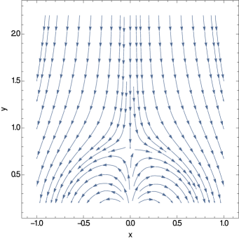
Figure 1: 2D potential field zoomed-in to the dipole region.

4 Examples

We wish to stress that the equations for the transformation of the current derived in Sects. 3.1 and 3.2 are generally valid and limited to neither a particular initial physical scenario nor to a specific flow pattern, determined by $M_{A}$. In the following, for pure demonstration purpose, we chose two specific ground states, i.e. MHS states, one for a 2D equilibrium and the other for a 2.5D equilibrium. To each specific flow patterns are applied and the transformed current is computed. The Mach number profiles are chosen such that significant current fragmentation is achieved. Current fragmentation is an indispensable physical process for plasma heating applications, e.g., in the solar corona. We thus pick a physical environment for our model calculations which can be considered representative for (subareas) of coronal arcade structures and loops.

4.1 2D scenario

We start from a 2D potential field as a current free MHS state. To simulate the footpoint region of a typical solar arcade or of some other mono-polar domain of the magnetic field in the solar atmosphere we superimpose a line-dipole, which is located at the solar surface, and a homogeneous field. Our coordinate system has its origin on the solar surface with the $x$- and $z$-axis being tangential to the surface and the $y$-axis perpendicular.

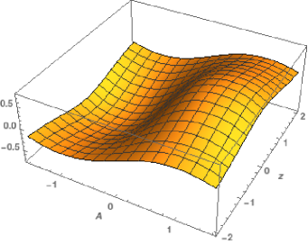
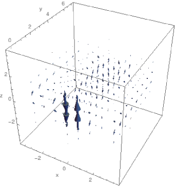
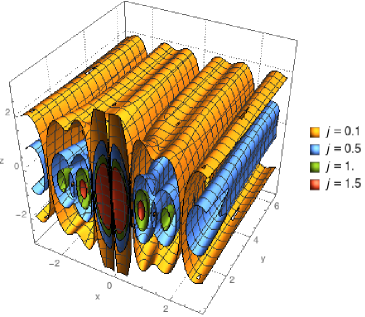
Figure 2: Mach number profile (top) for the values of $k_{1}=1.57$ and $k_{2}=0$ plotted over the phase space $f\equiv A(x,y)$ and $g\equiv z$, current density vectors (mid) and isocontours of the current (bottom) for this Mach number profile

The field configuration is computed from the complex potential ${\cal A}\left(u\right)$ with $u=x+iy$ and

$${\cal A}\left(u\right)=iu-\frac{0.6i}{u}\,,$$ (47)

where the imaginary part of ${\cal A}$ is the magnetic flux function $A$

$$\Im({\cal A})=A(x,y)=x-\frac{0.6x}{x^{2}+y^{2}}\,.$$ (48)

The magnetic field then results to

$$B_{xS} = \frac{\partial A}{\partial y}=-\frac{1.2xy}{\left(x^{2}+y^{2}\right)^{2}}$$ (49)

$$B_{yS} = -\frac{\partial A}{\partial x}=-1+\frac{0.6y^{2}-0.6x^{2}}{\left(x^{2}+y^{2}\right)^{2}}\,.$$ (50)

This process delivers an X-type magnetic null point at $(x_{N},y_{N})=(0,\sqrt{3/5})$ in the upper half domain $y>0$. For illustration, the field lines of this particular potential field are shown in Figure 1.

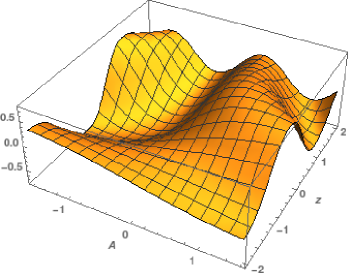
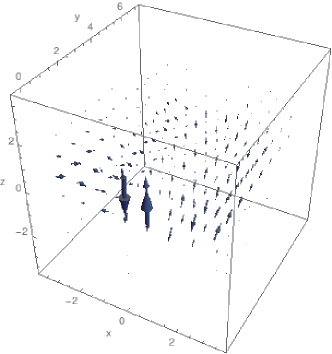
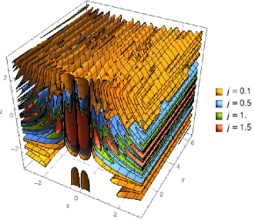
Figure 3: Mach number profile (top) for the values of $k_{1}=1.57$ and $k_{2}=0.75$ plotted over the phase space $f\equiv A(x,y)$ and $g\equiv z$, current density vectors (mid) and isocontours of the current (bottom) for this Mach number profile.

The general form of the Mach number profile is given by Equation (23). We chose the function ${\cal M}(f,g)\equiv{\cal M}(A,z)$ in the following parametrized form

$${\cal M}(A,z)=\left[\frac{\sin(k_{1}A(1+k_{2}z))}{1+0.5z^{2}}\right]\,,$$ (51)

where the parameters $k_{1}$ and $k_{2}$ are constants. The choice of the sine function guarantees that the Mach number profile has a wavy shape, which causes gradients that produce great spacial variations in the resulting current. A non-constant Mach number that varies spatially on small scales is motivated by the analogy to perturbation theory. Every flow induced by the Mach number should optimize the current distribution to guarantee efficient dissipation of magnetic energy in form of Ohmic heating.

To study the influence of the choice of the Mach number profile on the resulting current structure, we compute two scenarios, one of them is symmetric with respect to the $z=0$ plane, the other one asymmetric. For the first, symmetric case we set $k_{1}=1.57$ and $k_{2}=0$. With these values the Mach number profile, which is shown in Figure 2, has a very smooth, only mildly varying shape. Application of this Mach number profile to the MHS state results in the formation of quasi-3D tube-like current filaments. A selection of current isocontours of these filaments is depicted in the bottom panel of Figure 2. The current of this MHD flow has a 3D character, as can be seen in the middle panel of Figure 2 where we plot the current density vector. The current density is strongest in the vicinity of the dipole field and around $z=0$.

For the second example, we use the following values for the constants in Equation (51): $k_{1}=1.57$ and $k_{2}=0.75$. The resulting Mach number profile is depicted in the top panel of Figure 3, the isocontours of the current filaments and the current density vector are shown in the bottom and middle panels of Figure 3, respectively. The choice of $k_{2}\neq 0$ results in an asymmetry with respect to the $z=0$ plane in the Mach number profile. In addition, the profile displays clearly stronger gradients. This leads to currents with very narrow, highly filamentary structures as can be seen in the image of the isocontours.

4.2 2.5D scenario

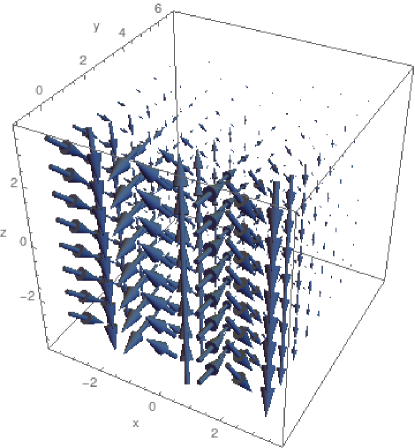
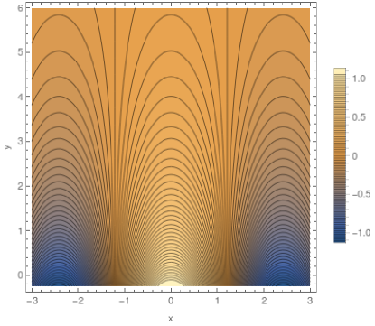
Figure 4: Direction and strength of the initial force-free magnetic field (top) and the projection of the field lines of this field (bottom) into the $x$-$y$-plane in the 2.5D case. Color coding refers to magnetic flux (function).

For the 2.5D scenario we start from a linear force-free field as initial MHS equilibrium. Such fields are typically chosen to model coronal magnetic fields (see the review by Wiegelmann & Sakurai, 2012). We restrict to constant force-free fields, which means that the electric current density is given by $\textbf{{j}}=c\textbf{{B}}$ where $c$ is a constant, and represent our force-free field with the Euler potentials $f$ and $g$

$$\textbf{{B}}_{S} = {\boldsymbol{\nabla}}f{\boldsymbol{\times}}{\boldsymbol{\nabla}}g$$ (52)

$$f = B_{0}\cos\left(kx\right)\exp\left(-\nu y\right)$$ (53)

$$g = z+\frac{c}{\nu}x\,,$$ (54)

where $\nu=\sqrt{k^{2}-c^{2}}$. For the presented case, we fix the constants at the following values: $B_{0}=1$, $k=1.3$, and $c=1.2$.

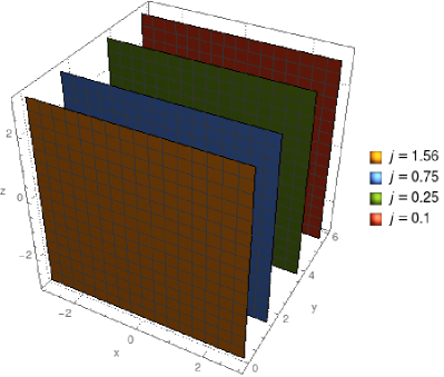
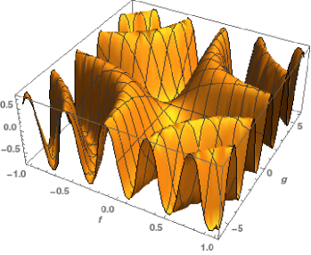
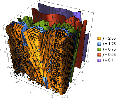
Figure 5: Isosurfaces of the initial current density (top), Mach number profile (mid), and isosurfaces of the transformed current density (bottom) in the 2.5D case.

We chose the Euler potentials such that $f$ represents a component of the Fourier expansion of this force-free field (see, e.g., Wiegelmann, 1998), and the second term of $g$ describes the component of the field in $z$-direction, i.e., the toroidal component, where $z$ is chosen as the invariant direction. The force-free magnetic field is shown in Figure 4, where we plot its direction and strength (top panel) and the projection of the field lines into the $x$-$y$-plane (bottom panel). The magnetic field is strongest for $y=0$ and decays with increasing values of $y$. Consequently, also the current density has its maximum at $y=0$. Moreover, with the chosen representation of the Euler potentials, the current density is a pure function of $y$ and decays exponentially. Selected isocontours of this initial current density are shown in the top panel of Figure 5. Obviously, the isocontours are parallel to the $x$-$z$-plane and the maximum value of the current density is reached for $y=0$ where it has a numerical value of 1.56.

We define the Mach number profile in the following form

$$M_{A}=\tanh\left[\sin(2.5fg)\right]\,,$$ (55)

to provide a spatially strongly oscillating function. It is shown in the middle panel of Figure 5. The results from applying this profile to the static equilibrium are shown in the bottom panel of Figure 5. Obviously, the former isocontour planes of the current density display now wavy structures with dependency in the initially invariant direction and their surfaces are enlarged. Moreover, the numerical values of the mapped current density are larger, especially in the regions of high initial values of the magnetic field strength. These properties of the mapped current density (enlargement of both the isocontour surfaces and their numerical values) favor such kind of configurations for Ohmic dissipation.

5 Discussion and Conclusions

We present a general parametrization for the calculation of non-canonical transformations in the sub-Alfvénic case. This parametrization provides an ideal tool to calculate all possible transformations for a given MHS equilibrium, represented by the Euler potentials $f$ and $g$. We apply this parametrization on 2D and 2.5D MHS equilibria and obtain symmetry breaking of the current, resulting in three current components depending on all three spatial coordinates. The symmetry breaking implies that the magnetic field lines can have high symmetry and are ordered and non-chaotic (non-ergodic), but due to strong gradients of the flow the current distribution appears strongly shredded, displaying complex lamination. The additional fragmentation of the current filaments from Figure 2 into the highly filamentary structures seen in Figure 3 which is caused by only a slight change in the Mach number profile, shows that it is possible to obtain highly complex current distributions from an initially stationary and ordered magnetic field. These results demonstrate that to achieve strong currents, it is sufficient to have ordered fields and ordered flows. These currents are in principle suitable to trigger magnetic reconnection or pure Ohmic heating. Moreover, our results imply that in contrast to Parker’s idea of coronal heating, pure singular current sheets, i.e. tangential discontinuities, are not necessarily required. It is sufficient to have current sheets that are strong enough to overcome instability thresholds for magnetic reconnection or to achieve required Ohmic heating rates. Such currents can easily be achieved with our model of symmetry breaking. However, it would be desirable to obtain those current density distributions which have sufficient strength and a suitable structure at the right locations to trigger current driven instabilities. For this, an optimization procedure for the Mach number profile needs to be developed.

Another aspect of our studies is devoted to the question whether force-free fields are generic. Although flows supporting force-free states have been a subject of investigation already in the seventies (Sreenivasan, 1973; Sreenivasan & Thompson, 1974), only a limited set of such flows could be calculated. However, these flows must obey very specific conditions, which means that the force-free state is not arbitrarily free, and even the force-free parameter $\alpha$ has to obey severe restrictions. As an example, Sreenivasan & Thompson (1974) found that for axis-symmetric cases $\alpha$ must be a function of space and time, while recent studies of Paccagnella & Guazzotto (2011) revealed that confined solutions which necessarily need a monotonically decreasing pressure, cannot exist.

Our analysis confirms and reinforces these previous findings. Moreover, it shows that force-free magnetic fields can be maintained by flows either only for specific geometries or for constant Mach numbers.

References

- Bingert & Peter (2011) Bingert, S., & Peter, H. 2011, A&A, 530, A112
- Bogoyavlenskij (2001) Bogoyavlenskij, O. I. 2001, Physics Letters A, 291, 256
- Bogoyavlenskij (2002) —. 2002, Phys. Rev. E, 66, 056410
- Bourdin et al. (2013) Bourdin, P.-A., Bingert, S., & Peter, H. 2013, A&A, 555, A123
- Cicogna & Pegoraro (2015) Cicogna, G., & Pegoraro, F. 2015, Physics of Plasmas, 22, 022520
- Gebhardt & Kiessling (1992) Gebhardt, U., & Kiessling, M. 1992, Physics of Fluids B, 4, 1689
- Grad & Rubin (1958) Grad, H., & Rubin, H. 1958, in Proceedings of the Second United Nations International Conference on the Peaceful Uses of Atomic Energy, Vol. 31, Theoretical and Experimental Aspects of Controlled Nuclear Fusion, 190–197
- Hansteen et al. (2015) Hansteen, V., Guerreiro, N., De Pontieu, B., & Carlsson, M. 2015, ApJ, 811, 106
- Harvey & Harvey (1976) Harvey, K. L., & Harvey, J. W. 1976, Sol. Phys., 47, 233
- Jelínek et al. (2015) Jelínek, P., Karlický, M., & Murawski, K. 2015, ApJ, 812, 105
- Khater & Moawad (2005) Khater, A. H., & Moawad, S. M. 2005, Physics of Plasmas, 12, 052902
- Kippenhahn & Moellenhoff (1975) Kippenhahn, R., & Moellenhoff, C. 1975, Mannheim West Germany Bibliographisches Institut AG
- Kotrč et al. (2013) Kotrč, P., Bárta, M., Schwartz, P., et al. 2013, Sol. Phys., 284, 447
- Leake et al. (2014) Leake, J. E., Linton, M. G., & Antiochos, S. K. 2014, ApJ, 787, 46
- Low (1982) Low, B. C. 1982, ApJ, 263, 952
- Low (1985) —. 1985, Sol. Phys., 100, 309
- Low (1991) —. 1991, ApJ, 370, 427
- Low (2010) —. 2010, ApJ, 718, 717
- Lüst & Schlüter (1957) Lüst, R., & Schlüter, A. 1957, Zeitschrift Naturforschung Teil A, 12, 850
- Manchester (2003) Manchester, W. 2003, Journal of Geophysical Research (Space Physics), 108, 1162
- Marsch et al. (2004) Marsch, E., Wiegelmann, T., & Xia, L. D. 2004, A&A, 428, 629
- Moffatt (1978) Moffatt, H. K. 1978, Magnetic field generation in electrically conducting fluids
- Neukirch (1995) Neukirch, T. 1995, A&A, 301, 628
- Neukirch (1997) —. 1997, A&A, 325, 847
- Nickeler et al. (2006) Nickeler, D. H., Goedbloed, J. P., & Fahr, H.-J. 2006, A&A, 454, 797
- Nickeler et al. (2013) Nickeler, D. H., Karlický, M., Wiegelmann, T., & Kraus, M. 2013, A&A, 556, A61
- Nickeler et al. (2014) —. 2014, A&A, 569, A44
- Nickeler & Wiegelmann (2010) Nickeler, D. H., & Wiegelmann, T. 2010, Annales Geophysicae, 28, 1523
- Nickeler & Wiegelmann (2012) —. 2012, Annales Geophysicae, 30, 545
- Paccagnella & Guazzotto (2011) Paccagnella, R., & Guazzotto, L. 2011, Plasma Physics and Controlled Fusion, 53, 095013
- Parker (1972) Parker, E. N. 1972, ApJ, 174, 499
- Parker (1983a) —. 1983a, ApJ, 264, 642
- Parker (1983b) —. 1983b, ApJ, 264, 635
- Parker (1988) —. 1988, ApJ, 330, 474
- Parker (2012) —. 2012, Astrophysics and Space Science Proceedings, 33, 3
- Parnell & De Moortel (2012) Parnell, C. E., & De Moortel, I. 2012, Philosophical Transactions of the Royal Society of London Series A, 370, 3217
- Peter et al. (2015) Peter, H., Warnecke, J., Chitta, L. P., & Cameron, R. H. 2015, A&A, 584, A68
- Petrie & Neukirch (1999) Petrie, G. J. D., & Neukirch, T. 1999, Geophysical and Astrophysical Fluid Dynamics, 91, 269
- Petrie et al. (2005) Petrie, G. J. D., Tsinganos, K., & Neukirch, T. 2005, A&A, 429, 1081
- Petrie et al. (2002) Petrie, G. J. D., Vlahakis, N., & Tsinganos, K. 2002, A&A, 382, 1081
- Pongkitiwanichakul et al. (2015) Pongkitiwanichakul, P., Cattaneo, F., Boldyrev, S., Mason, J., & Perez, J. C. 2015, MNRAS, 454, 1503
- Prior & Yeates (2016) Prior, C., & Yeates, A. R. 2016, A&A, 587, A125
- Sakurai (1979) Sakurai, T. 1979, PASJ, 31, 209
- Schindler (2006) Schindler, K. 2006, Physics of Space Plasma Activity, 522, doi:10.2277/0521858976
- Shafranov (1958) Shafranov, V. D. 1958, Soviet Journal of Experimental and Theoretical Physics, 6, 545
- Solov’ev & Kirichek (2015) Solov’ev, A. A., & Kirichek, E. A. 2015, Astronomy Letters, 41, 211
- Sreenivasan (1973) Sreenivasan, S. R. 1973, Physica, 67, 323
- Sreenivasan & Thompson (1974) Sreenivasan, S. R., & Thompson, D. L. 1974, Physica, 78, 321
- Stern (1970) Stern, D. P. 1970, American Journal of Physics, 38, 494
- Toriumi et al. (2013) Toriumi, S., Iida, Y., Bamba, Y., et al. 2013, ApJ, 773, 128
- Tsinganos et al. (1993) Tsinganos, K., Surlantzis, G., & Priest, E. R. 1993, A&A, 275, 613
- Tsinganos (1982) Tsinganos, K. C. 1982, ApJ, 259, 832
- Švanda & Karlický (2016) Švanda, M., & Karlický, M. 2016, ApJ, 831, 9
- Wallace et al. (2010) Wallace, A. J., Harra, L. K., van Driel-Gesztelyi, L., Green, L. M., & Matthews, S. A. 2010, Sol. Phys., 267, 361
- Wiegelmann (1998) Wiegelmann, T. 1998, Physica Scripta Volume T, 74, 77
- Wiegelmann & Sakurai (2012) Wiegelmann, T., & Sakurai, T. 2012, Living Reviews in Solar Physics, 9, 5
- Wiegelmann et al. (2005) Wiegelmann, T., Xia, L. D., & Marsch, E. 2005, A&A, 432, L1
- Wilmot-Smith et al. (2011) Wilmot-Smith, A. L., Pontin, D. I., Yeates, A. R., & Hornig, G. 2011, A&A, 536, A67
- Winebarger et al. (2001) Winebarger, A. R., DeLuca, E. E., & Golub, L. 2001, ApJ, 553, L81
- Winebarger et al. (2002) Winebarger, A. R., Warren, H., van Ballegooijen, A., DeLuca, E. E., & Golub, L. 2002, ApJ, 567, L89
- Yoshimura et al. (1971) Yoshimura, H., Tanaka, K., Skimizu, M., & Hiei, E. 1971, PASJ, 23, 443