Causal inference with confounders missing not at random

Abstract

It is important to draw causal inference from observational studies, which, however, becomes challenging if the confounders have missing values. Generally, causal effects are not identifiable if the confounders are missing not at random. We propose a novel framework to nonparametrically identify causal effects with confounders subject to an outcome-independent missingness, that is, the missing data mechanism is independent of the outcome, given the treatment and possibly missing confounders. We then propose a nonparametric two-stage least squares estimator and a parametric estimator for causal effects.

Keywords: Completeness; Ill-posed inverse problem; Integral equation; Outcome-independent missingness

1 Introduction

Causal inference plays important roles in biomedical studies and social sciences. If all the confounders of the treatment-outcome relationship are observed, one can use standard techniques, such as propensity score matching, subclassification and weighting to adjust for confounding (e.g., Rosenbaum and Rubin, 1983; Imbens and Rubin, 2015).

Much less work has been done to deal with the case when confounders have missing values. Rosenbaum and Rubin (1984) and D’Agostino Jr and Rubin (2000) developed a generalized propensity score approach. Under a modified unconfoundedness assumption, they showed that adjusting for the missing pattern and the observed values of confounders removes all confounding bias, and hence the causal effects are identifiable. Moreover, the balancing property of the propensity score carries over to the generalized propensity score. Standard propensity score methods can hence be used to estimate the causal effects. However, the modified unconfoundedness assumption implies that units may have different confounders depending on the missing pattern, which is often hard to justify scientifically. An alternative approach assumes that the confounders are missing at random (Rubin, 1976). Under this assumption, both the full data distribution and causal effects are identifiable, and multiple imputation can provide reasonable estimates of the causal effects (Rubin, 1987; Qu and Lipkovich, 2009; Crowe et al., 2010; Mitra and Reiter, 2011; Seaman and White, 2014). In practice, however, the missing pattern often depends on the missing values themselves, a scenario commonly known as missing not at random (Rubin, 1976). Previous multiple imputation methods may fail to provide valid inference in this scenario. See Mattei (2009) for a comparison of various methods and Lu and Ashmead (2018) for a sensitivity analysis.

Causal inference with confounders missing not at random is challenging because neither the full data distribution nor the causal effects are identifiable without further assumptions. We consider a novel setting where the confounders are subject to an outcome-independent missingness, that is, the missing data mechanism is independent of the outcome, given the treatment and possibly missing confounders. This outcome-independent missingness is more plausible if the outcome happens after the covariate measurements and missing data indicators. To identify the causal effects under this setting, we formulate the identification problem as solving an integral equation, and show that identification of the full data distribution is equivalent to unique existence of the solution to an inverse problem. This new perspective allows us to establish a general condition for identifiability of the causal effects. Our condition generalizes the existing results for a discrete covariate and outcome (Ding and Geng, 2014). Motivated by the identification result, we develop a nonparametric two-stage least squares estimator by solving the sample analog of the integral equation. To avoid the curse of dimensionality, we further develop parametric likelihood-based methods.

2 Setup and assumptions

2.1 Potential outcomes, causal effects, and unconfoundedness

We use potential outcomes to define causal effects. Suppose that the binary treatment is $A\in\{0,1\}$, with $0$ and $1$ being the labels for the control and active treatments, respectively. Each level of treatment $a$ corresponds to a potential outcome $Y(a)$, representing the outcome had the subject, possibly contrary to the fact, been given treatment $a$. The observed outcome is $Y=Y(A)=AY(1)+(1-A)Y(0)$. Let $X=(X_{1},\ldots,X_{p})$ be a vector of $p$-dimensional pre-treatment covariates. We assume that a sample of size $n$ consists of independent and identically distributed draws from the distribution of $\{A,X,Y(0),Y(1)\}$. The covariate-specific causal effect is $\tau(X)=E\{Y(1)-Y(0)\mid X\}$, and the average causal effect is $\tau=E\{Y(1)-Y(0)\}=E\{\tau(X)\}$. We focus on $\tau$, and a similar discussion applies to the average causal effect on the treated $\tau_{\mathrm{ATT}}=E\{Y(1)-Y(0)\mid A=1\}=E\{\tau(X)\mid A=1\}$. The following assumptions are standard in causal inference with observational studies (Rosenbaum and Rubin, 1983).

Assumption 1

$\{Y(0),Y(1)\}\mathbin{\mathchoice{\hbox to0.0pt{\hbox{$\displaystyle\perp$}\hss}\kern 3.46875pt{}\kern 3.46875pt\hbox{$\displaystyle\perp$}}{\hbox to0.0pt{\hbox{$\textstyle\perp$}\hss}\kern 3.46875pt{}\kern 3.46875pt\hbox{$\textstyle\perp$}}{\hbox to0.0pt{\hbox{$\scriptstyle\perp$}\hss}\kern 2.36812pt{}\kern 2.36812pt\hbox{$\scriptstyle\perp$}}{\hbox to0.0pt{\hbox{$\scriptscriptstyle\perp$}\hss}\kern 1.63437pt{}\kern 1.63437pt\hbox{$\scriptscriptstyle\perp$}}}A\mid X$.

Assumption 2

There exist constants $c_{1}$ and $c_{2}$ such that $0<c_{1}\leq e(X)\leq c_{2}<1$ almost surely, where $e(X)=\mathrm{pr}(A=1\mid X)$ is the propensity score.

Under Assumptions 1 and 2, $\tau=E\{E(Y\mid A=1,X)-E(Y\mid A=0,X)\}$ is identifiable from the joint distribution of observed data $(A,X,Y)$. Rosenbaum and Rubin (1983) showed that $\{Y(0),Y(1)\}\mathbin{\mathchoice{\hbox to0.0pt{\hbox{$\displaystyle\perp$}\hss}\kern 3.46875pt{}\kern 3.46875pt\hbox{$\displaystyle\perp$}}{\hbox to0.0pt{\hbox{$\textstyle\perp$}\hss}\kern 3.46875pt{}\kern 3.46875pt\hbox{$\textstyle\perp$}}{\hbox to0.0pt{\hbox{$\scriptstyle\perp$}\hss}\kern 2.36812pt{}\kern 2.36812pt\hbox{$\scriptstyle\perp$}}{\hbox to0.0pt{\hbox{$\scriptscriptstyle\perp$}\hss}\kern 1.63437pt{}\kern 1.63437pt\hbox{$\scriptscriptstyle\perp$}}}A\mid e(X)$, so adjusting for the propensity score removes all confounding. We can estimate $\tau$ through propensity score matching, subclassification or weighting.

2.2 Confounders with missing values and the generalized propensity score

We consider the case where $X$ contains missing values. Let $R=(R_{1},\ldots,R_{p})$ be the vector of missing indicators such that $R_{j}=1$ if the $j$th component $X_{j}$ is observed and $0$ if $X_{j}$ is missing. Let $\mathcal{R}$ be the set of all possible values of $R$. We use $1_{p}$ to denote the $p$-vector of $1$’s and $0_{p}$ to denote the $p$-vector of $0$’s. The missingness pattern $R=r\in\mathcal{R}$ partitions the covariates $X$ into $X_{r}$ and $X_{\overline{r}}$, the observed and missing parts of $X$, respectively. Using Rubin (1976)’s notation, $X_{{R}}=X_{\text{obs}}$ and $X_{{\overline{R}}}=X_{\text{mis}}$ are the realized observed and missing covariates, respectively. For example, if $R_{1}=1$ and $R_{j}=0$ for $j=2,\ldots,p$, then $X_{{R}}=X_{1}$ and $X_{{\overline{R}}}=(X_{2},\ldots,X_{p})$. With missing data, assume that we have independent and identically distributed draws from $\{A,X,Y(1),Y(0),R\}$. Rosenbaum and Rubin (1984) introduced the following modified unconfoundedness assumption.

Assumption 3

$\{Y(0),Y(1)\}\mathbin{\mathchoice{\hbox to0.0pt{\hbox{$\displaystyle\perp$}\hss}\kern 3.46875pt{}\kern 3.46875pt\hbox{$\displaystyle\perp$}}{\hbox to0.0pt{\hbox{$\textstyle\perp$}\hss}\kern 3.46875pt{}\kern 3.46875pt\hbox{$\textstyle\perp$}}{\hbox to0.0pt{\hbox{$\scriptstyle\perp$}\hss}\kern 2.36812pt{}\kern 2.36812pt\hbox{$\scriptstyle\perp$}}{\hbox to0.0pt{\hbox{$\scriptscriptstyle\perp$}\hss}\kern 1.63437pt{}\kern 1.63437pt\hbox{$\scriptscriptstyle\perp$}}}A\mid(X_{{R}},R)$.

Under Assumption 3, the generalized propensity score $e(X_{{R}},R)=\mathrm{pr}(A=1\mid X_{{R}},R)$ plays the same role as the usual propensity score $e(X)=\mathrm{pr}(A=1\mid X)$ in the settings without missing covariates. Rosenbaum and Rubin (1984) showed that adjusting for $e(X_{{R}},R)$ balances $(X_{{R}},R)$ and removes all confounding on average. Their approach has the advantage of requiring no assumptions on the missing data mechanism of $X$ for the identification of causal effects. However, their approach implies that a pre-treatment covariate can be a confounder when it is observed but not a confounder when it is missing. This is often hard to justify scientifically. Moreover, if the covariate measurement occurs after the treatment assignment, then $R$ is a post-treatment variable affected by $A$. In this case, even if $A$ is completely randomized, Assumption 3 is unlikely to hold conditioning on the post-treatment variable $R$ (Frangakis and Rubin, 2002).

2.3 Missing data mechanisms of the confounders

Without Assumption 3, one needs to impose assumptions on the missing data mechanism. We now describe existing estimation methods under different missingness mechanisms of the confounders. The first one is missing completely at random (Rubin, 1976).

Assumption 4 (Missing completely at random)

$R\mathbin{\mathchoice{\hbox to0.0pt{\hbox{$\displaystyle\perp$}\hss}\kern 3.46875pt{}\kern 3.46875pt\hbox{$\displaystyle\perp$}}{\hbox to0.0pt{\hbox{$\textstyle\perp$}\hss}\kern 3.46875pt{}\kern 3.46875pt\hbox{$\textstyle\perp$}}{\hbox to0.0pt{\hbox{$\scriptstyle\perp$}\hss}\kern 2.36812pt{}\kern 2.36812pt\hbox{$\scriptstyle\perp$}}{\hbox to0.0pt{\hbox{$\scriptscriptstyle\perp$}\hss}\kern 1.63437pt{}\kern 1.63437pt\hbox{$\scriptscriptstyle\perp$}}}(A,X,Y)$.

Assumption 4 requires that the missingness of confounders is independent of all variables $(A,X,Y)$. It implies $\tau=E\{\tau(X)\mid R=1_{p}\}$ and thus justifies the complete-case analysis that uses only the units with fully observed confounders. This complete-case analysis is however inefficient by discarding all units with missing confounders. Moreover, confounders are rarely missing completely at random.

The second one is missing at random (Rubin, 1976).

Assumption 5 (Missing at random)

$R\mathbin{\mathchoice{\hbox to0.0pt{\hbox{$\displaystyle\perp$}\hss}\kern 3.46875pt{}\kern 3.46875pt\hbox{$\displaystyle\perp$}}{\hbox to0.0pt{\hbox{$\textstyle\perp$}\hss}\kern 3.46875pt{}\kern 3.46875pt\hbox{$\textstyle\perp$}}{\hbox to0.0pt{\hbox{$\scriptstyle\perp$}\hss}\kern 2.36812pt{}\kern 2.36812pt\hbox{$\scriptstyle\perp$}}{\hbox to0.0pt{\hbox{$\scriptscriptstyle\perp$}\hss}\kern 1.63437pt{}\kern 1.63437pt\hbox{$\scriptscriptstyle\perp$}}}X\mid(A,Y)$.

Under Assumption 5, conditioning on the treatment and outcome, the missing mechanism of confounders is independent of the missing values themselves. Assumption 5 implies $f(A,X,Y)=f(A,Y)f(X\mid A,Y,R=1_{p})$, and therefore, the joint distribution and its functionals including $\tau$ are all identifiable. Rubin (1976) showed that we can ignore the missing data mechanism in the likelihood-based and Bayesian inferences under Assumption 5. In this case, multiple imputation is a popular tool for causal inference (e.g., Qu and Lipkovich, 2009; Crowe et al., 2010; Mitra and Reiter, 2011; Seaman and White, 2014). Although Rubin (2007) suggested not using the outcome in the design of an observational study, imputing the missing confounders based on $f(X_{\overline{R}}\mid X_{R},A,Y)\propto f(X)f(A\mid X)f(Y\mid A,X)$ involves an outcome model in general (U.S. Department of Education, 2017).

However, missingness at random is not plausible if the missing pattern depends on the missing values themselves. Instead, we consider the following missing data mechanism.

Assumption 6 (Outcome-independent missingness)

$R\mathbin{\mathchoice{\hbox to0.0pt{\hbox{$\displaystyle\perp$}\hss}\kern 3.46875pt{}\kern 3.46875pt\hbox{$\displaystyle\perp$}}{\hbox to0.0pt{\hbox{$\textstyle\perp$}\hss}\kern 3.46875pt{}\kern 3.46875pt\hbox{$\textstyle\perp$}}{\hbox to0.0pt{\hbox{$\scriptstyle\perp$}\hss}\kern 2.36812pt{}\kern 2.36812pt\hbox{$\scriptstyle\perp$}}{\hbox to0.0pt{\hbox{$\scriptscriptstyle\perp$}\hss}\kern 1.63437pt{}\kern 1.63437pt\hbox{$\scriptscriptstyle\perp$}}}Y\mid(A,X)$.

Assumption 6 is plausible for prospective observational studies with $X$ measured long before the outcome takes place. Moreover, Assumption 6 is more plausible than Assumptions 4 and 5 for a certain class of examples where a potentially hazardous exposure has come under substantial scrutiny, data may be collected more comprehensively for exposed than for unexposed subjects; e.g., for the water crisis in Flint, Michigan U.S. (Hanna-Attisha et al., 2016), potentially exposed children and neighborhoods will have been more carefully measured than unexposed children and neighborhoods that will eventually serve as their comparisons.

Figure 1 is a causal diagram (Pearl, 1995) illustrating Assumptions 1 and 6. Graphically, $A$ and $Y$ have no common parents except for $X$, encoding Assumption 1, and $R$ and $Y$ have no common parents except $A$ and $X$, encoding Assumption 6. Our framework allows for unmeasured common causes of $R$ and $A$, and the dependence of $R$ on the missing confounders $X_{{\overline{R}}}$. Moreover, it allows $R$ to be a post-treatment variable affected by $A$.

Assumption 6 exploits the temporal orders of $(A,X,R)$ and $Y$. It restricts the joint distribution of $(A,X,R,Y)$ which makes nonparametric identification possible. This is a feature of the missingness of confounders. In contrast, the missingness of outcome may depend on all variables happening before.

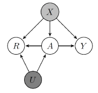
Figure 1: A direct acyclic graph illustrating Assumptions 1 and 6. White nodes represent observed variables, the light grey node represents the variable with missing values, and the dark node represents an unmeasured variable $U$.

We also make the following assumption to rule out degeneracy of the missing data mechanism.

Assumption 7

$\mathrm{pr}(R=1_{p}\mid A,X,Y)>c_{3}>0$ almost surely for some constant $c_{3}.$

3 Nonparametric identification

3.1 Identification strategy

Assume that the distribution of $(A,X,Y,R)$ is absolutely continuous with respect to some measure, with $f(A,X,Y,R)$ being the density or probability mass function. Under Assumptions 1 and 2, the key is to identify the joint distribution of $f(A,X,Y)$ because $\tau$ is its functional. The following identity relates the full data distribution to the observed data distribution:

$$f(A,X,Y,R=1_{p})=f(A,X,Y)\mathrm{pr}(R=1_{p}\mid A,X,Y).$$ (1)

The left-hand side of (1) is identifiable under Assumption 7. Therefore, the identification of $f(A,X,Y)$ relies on the identification of $\mathrm{pr}(R=1_{p}\mid A,X,Y)$. We now discuss how to identify $\mathrm{pr}(R=1_{p}\mid A,X,Y)=\mathrm{pr}(R=1_{p}\mid A,X)$ under Assumption 6.

3.2 Integral equation representation

Under Assumption 6, let

$$\xi_{ra}(X)=\frac{\mathrm{pr}(R=r\mid A=a,X,Y)}{\mathrm{pr}(R=1_{p}\mid A=a,X,Y)}=\frac{\mathrm{pr}(R=r\mid A=a,X)}{\mathrm{pr}(R=1_{p}\mid A=a,X)},\quad(a=0,1;r\in\mathcal{R}).$$

It then suffices to identify $\xi_{ra}(X)$, because it determines the missing data mechanism via

$$\mathrm{pr}(R=r\mid A=a,X,Y)=\frac{\mathrm{pr}(R=r\mid A=a,X,Y)}{\sum_{r^{\prime}\in\mathcal{R}}\mathrm{pr}(R=r^{\prime}\mid A=a,X,Y)}=\frac{\xi_{ra}(X)}{\sum_{r^{\prime}\in\mathcal{R}}\xi_{r^{\prime}a}(X)}.$$ (2)

The following theorem shows that $\xi_{ra}(X)$ is a key term connecting the observed data distribution $f(A,X_{{r}},Y,R)$ and the complete-case distribution $f(A,X,Y,R=1_{p})$. Throughout the paper, we use $\nu(\cdot)$ to denote a generic measure, e.g., the Lebesgue measure for continuous variable and the counting measure for discrete variable.

Theorem 1

Under Assumption 6, for any $r$ and $a$, the following integral equation holds:

$$f(A=a,X_{{r}},Y,R=r)=\int\xi_{ra}(X)f(A=a,X,Y,R=1_{p})\mathrm{d}\nu(X_{{\overline{r}}}).$$ (3)

Proof.  The conclusion follows because observed data distribution is the complete data distribution averaged over the missing data:

$$f(A=a,X_{{r}},Y,R=r) = \int f(A=a,X,Y,R=r)\mathrm{d}\nu(X_{{\overline{r}}})$$

$$= \int\frac{\mathrm{pr}(R=r\mid A=a,X,Y)}{\mathrm{pr}(R=1_{p}\mid A=a,X,Y)}f(A=a,X,Y,R=1_{p})\mathrm{d}\nu(X_{{\overline{r}}})$$

$$= \int\xi_{ra}(X)f(A=a,X,Y,R=1_{p})\mathrm{d}\nu(X_{{\overline{r}}}).$$

Theorem 1 is the basis of our identification analysis. In (3), $f(A=a,X_{{r}},Y,R=r)$ and $f(A=a,X,Y,R=1_{p})$ are identifiable from the observed data. We have thus turned the identification of $\xi_{ra}(X)$ to the problem of solving $\xi_{ra}(X)$ from (3). This requires additional technical assumptions below.

3.3 Bounded completeness and identification of the joint distribution

To motivate our identification conditions, we first consider the case with discrete $X$ and $Y$, where (3) becomes a linear system. To solve $\xi_{ra}(X)$ from (3), we need the linear system to be non-degenerate.

Proposition 1

Under Assumption 6, suppose that $X$ and $Y$ are discrete, and $X_{j}\in\{x_{j1},\ldots x_{jJ_{j}}\}$ for $j=1,\ldots,p$, and $Y\in\{y_{1},\ldots,y_{K}\}$. Let $q=J_{1}\times\cdots\times J_{p}$, and let $\Theta_{a}$ be a $K\times q$ matrix with the $k$-th row being $f(X,y_{k},R=1_{p},A=a)$ evaluated at all possible values of $X$. The distribution of $(A,X,Y,R)$ is identifiable if $\textup{Rank}(\Theta_{a})=q$ for $a=0,1$.

We relegate the proof to the Supplementary Material. For the special case with a binary $X$ and a discrete $Y$, the rank condition in Proposition 1 is equivalent to $X\mathbin{\mathchoice{\hbox to0.0pt{\hbox{$\displaystyle\perp$}\hss}\kern 3.46875pt{\not}\kern 3.46875pt\hbox{$\displaystyle\perp$}}{\hbox to0.0pt{\hbox{$\textstyle\perp$}\hss}\kern 3.46875pt{\not}\kern 3.46875pt\hbox{$\textstyle\perp$}}{\hbox to0.0pt{\hbox{$\scriptstyle\perp$}\hss}\kern 2.36812pt{\not}\kern 2.36812pt\hbox{$\scriptstyle\perp$}}{\hbox to0.0pt{\hbox{$\scriptscriptstyle\perp$}\hss}\kern 1.63437pt{\not}\kern 1.63437pt\hbox{$\scriptscriptstyle\perp$}}}Y\mid(A=a,R=1)$ for $a=0$ and $1$, which is testable based on the observed data (Ding and Geng, 2014). For general cases, we need to extend the rank condition that ensures the unique existence of $\xi_{ra}(X)$. We use the notion of bounded completeness for general $X$ and $Y$, which is related to the concept of a complete statistic (Lehmann and Scheffé, 1950; Newey and Powell, 2003). Below, we say that a function $g(x)$ is bounded in $\mathcal{L}_{1}$-metric if $\sup_{x}|g(x)|\leq c$ for some $0<c<\infty$.

Definition 1

A function $f(X,Y)$ is bounded complete in $Y$, if $\int g(X)f(X,Y)\mathrm{d}\nu(X)=0$ implies $g(X)=0$ almost surely for any measurable function $g(X)$ bounded in $\mathcal{L}_{1}$-metric.

D’Haultfoeuille (2011) gave sufficient conditions for the bounded completeness. It also appeared in other identification analyses such nonparametric instrumental variable regression models (Darolles et al., 2011) and measurement error models (An and Hu, 2012).

We invoke the following assumption motivated by Theorem 1 and Definition 1.

Assumption 8

The joint distribution $f(A=a,X,Y,R=1_{p})$ is bounded complete in $Y$, for $a=0,1$.

Remark 1

When $X$ and $Y$ are discrete with finite supports, Assumption 8 is equivalent to the rank condition in Proposition 1. Moreover, Assumption 8 implies Assumption 2.

Under Assumption 7, Assumption 8 is sufficient to ensure the unique existence of $\xi_{ra}(X)$ from (3). We present the result in the following theorem.

Theorem 2

Under Assumptions 6–8, the distribution of $(A,X,Y,R)$ is identifiable.

Proof.  Suppose that $\xi_{ra}^{(1)}(X)$ and $\xi_{ra}^{(2)}(X)$ are two solutions to (3):

$$f(A=a,X_{{r}},Y,R=r)=\int\xi_{ra}^{(k)}(X)f(A=a,X,Y,R=1_{p})\mathrm{d}\nu(X_{{\overline{r}}}),\quad(k=1,2)$$

which imply $\int\{\xi_{ra}^{(1)}(X)-\xi_{ra}^{(2)}(X)\}f(A=a,X,Y,R=1_{p})\mathrm{d}\nu(X_{{\overline{r}}})=0.$ Integrating this identity with respect to $X_{{r}}$, we have

$$\int\{\xi_{ra}^{(1)}(X)-\xi_{ra}^{(2)}(X)\}f(A=a,X,Y,R=1_{p})\mathrm{d}\nu(X)=0.$$

Assumption 7 implies that $\xi_{ra}(X)$ is bounded in $\mathcal{L}_{1}$-metric, which further implies that $\xi_{ra}^{(1)}(X)-\xi_{ra}^{(2)}(X)$ is bounded in $\mathcal{L}_{1}$-metric. Under Assumption 8, Definition 1 implies that $\xi_{ra}^{(1)}(X)-\xi_{ra}^{(2)}(X)=0$ almost surely. Therefore, (3) has a unique solution $\xi_{ra}(X)$. Based on the definition of $\xi_{ra}(X)$, we can identify $\mathrm{pr}(R=1_{p}\mid A,X,Y)$ by (2). Finally, we identify $f(A,X,Y)$ through (1) as $f(A,X,Y)=f(A,X,Y,R=1_{p})/\mathrm{pr}(R=1_{p}\mid A,X,Y).$

If the distribution of $(A,X,Y)$ is identifiable, we can use a standard argument to show that $\tau$ and $\tau_{\mathrm{ATT}}$ are identifiable under Assumption 1. We give explicit identification formulas for $\tau$ and $\tau_{\mathrm{ATT}}$ in the next subsection, which are the basis for constructing the nonparametric estimator.

3.4 Nonparametric identification formulas for average causal effects

Under Assumptions 1, 6–8, we can identify $\tau$ and $\tau_{\mathrm{ATT}}$ in two steps. First,

$$\tau(X) = E(Y\mid A=1,X)-E(Y\mid A=0,X)$$ (4)

$$= E(Y\mid A=1,X,R=1_{p})-E(Y\mid A=0,X,R=1_{p}),$$ (5)

where (4) follows from Assumption 1, and (5) follows from Assumption 6. Therefore, we can identify $\tau(X)$ using a complete-case analysis based on (5).

Second, under Assumptions 6–8, Theorem 2 shows that the distribution of $(A,X,Y,R)$ is identifiable, which implies that the marginal distribution of $X$, $f(X)$, and the conditional distribution of $X$, $f(X\mid A=1)$, are also identifiable. Therefore, both $\tau=E\{\tau(X)\}$ and $\tau_{\mathrm{ATT}}=E\{\tau(X)\mid A=1\}$ are identifiable. The following theorem summarizes these results.

Theorem 3

Under Assumptions 1, 6–8, the average causal effect $\tau$ is identified by

$$\tau=\sum_{a=0}^{1}\int\tau(X)\frac{f(A=a,X,R=1_{p})}{\mathrm{pr}(R=1_{p}\mid A=a,X)}\mathrm{d}\nu(X),$$ (6)

and the average treatment effect on the treated $\tau_{\mathrm{ATT}}$ is identified by

$$\tau_{\mathrm{ATT}}=\int\tau(X)\frac{f(X,R=1_{p}\mid A=1)}{\mathrm{pr}(R=1_{p}\mid A=1,X)}\mathrm{d}\nu(X).$$ (7)

where $\tau(X)$ is identified by (5), $\mathrm{pr}(A=a,R=1_{p})$ and $f(A=a,X,R=1_{p})$ depend only on the observed data, and $\mathrm{pr}(R=1_{p}\mid A=a,X)$ can be identified from (3), for $a=0$ and $1$.

Proof.  First, we can identify the conditional distribution of $X$ given $A=a$ by

$$f(X\mid A=a)=\frac{f(X,R=1_{p}\mid A=a)}{\mathrm{pr}(R=1_{p}\mid A=a,X)},\quad(a=0,1).$$

Averaging $\tau(X)$ over $f(X\mid A=1)$, we obtain the identification formula (7).

Second, we can identify the marginal distribution of $X$ by

$$f(X)=\sum_{a=0}^{1}f(A=a,X)=\sum_{a=0}^{1}\frac{f(A=a,X,R=1_{p})}{\mathrm{pr}(R=1_{p}\mid A=a,X)}.$$

Averaging $\tau(X)$ over the above distribution, we obtain the identification formula (6).

4 Estimation of the average causal effect

4.1 Nonparametric two-stage least squares estimator

Theorem 3 shows the nonparametric identification formulas at the population level. Based on (6), we propose a nonparametric two-stage least squares estimator of $\tau$ with finite samples $(A_{i},X_{i},Y_{i},R_{i})_{i=1}^{n}$. We omit the estimation of $\tau_{\mathrm{ATT}}$. We estimate $\tau(X)$, $\mathrm{pr}(A=a,R=1_{p})$, $f(X\mid A=a,R=1_{p})$ and $\mathrm{pr}(R=1_{p}\mid A=a,X)$ by standard nonparametric methods, denoted by $\hat{\tau}(X)$, $\widehat{\mathrm{pr}}(A=a,R=1_{p})$, and $\hat{f}(X\mid A=a,R=1_{p})$, respectively. Thus, the key is to estimate $\mathrm{pr}(R=1_{p}\mid A=a,X)$, or, equivalently, $\xi_{ra}(X)$ based on (3).

In the first stage, we obtain $\hat{f}(X_{{r}},Y,R=r\mid A=a)$ and $\hat{f}(X,Y,R=1_{p}\mid A=a)$ as the nonparametric sample analogs of $f(X_{{r}},Y,R=r\mid A=a)$ and $f(X,Y,R=1_{p}\mid A=a)$. Replacing them in (3) leads to

$$\hat{f}(X_{{r}},Y,R=r\mid A=a)=\int\xi_{ra}(X)\hat{f}(X,Y,R=1_{p}\mid A=a)\mathrm{d}\nu(X_{{\overline{r}}}),$$ (8)

which is a Fredholm integral equation of the first kind. Solving (8) raises several challenges. First, although Theorem 2 shows that the population equation (3) has a unique solution, the sample equation (8) may not. Second, $\xi_{ra}(X)$ is an infinite-dimensional parameter, and its estimation often relies on some approximation. Third, solving $\xi_{ra}(X)$ from (8) is an ill-conditioned problem, in the sense that even a slight perturbation of $\hat{f}(X_{{r}},Y,R=r\mid A=a)$ and $\hat{f}(X,Y,R=1_{p}\mid A=a)$ can lead to a large variation in the solution for $\xi_{ra}(X)$. As a result, replacing $f(X_{{r}},Y,R=r\mid A=a)$ and $f(X,Y,R=1_{p}\mid A=a)$ (3) by their consistent estimators does not necessarily yield a consistent estimator of $\xi_{ra}(X)$ (Darolles et al., 2011).

To tackle these issues, we use the series approximation (Kress et al., 1999; Newey and Powell, 2003) in the second stage. Let the set $\mathcal{H}_{J}=\{h^{j}(X)=\exp(-X^{\mathrm{\scriptscriptstyle T}}X)X^{\lambda_{j}}:j=1,\ldots,J\}$ form a Hermite polynomial basis, where $X^{\lambda_{j}}=X_{1}^{\lambda_{j1}}\cdots X_{p}^{\lambda_{jp}}$, with $\lambda_{j}=(\lambda_{j1},\ldots,\lambda_{jp})$ and $|\lambda_{j}|=\sum_{l=1}^{p}\lambda_{jl}$ increasing in $j$. Let $\tilde{X}=\Sigma^{-1/2}(X-\mu)$ be a standardized version of $X$, where $\mu$ and $\Sigma$ are constant vector and matrix. We approximate $\xi_{ra}(X)$ by $\xi_{ra}(X)\approx\sum_{j=1}^{J}\beta_{ra}^{j}h^{j}(\tilde{X}).$ Thus, for each missing pattern $R=r$, we approximate (3) by

$$f(X_{{r}},Y,R=r\mid A=a) \approx \sum_{j=1}^{J}\beta_{ra}^{j}\int h^{j}(\tilde{X})f(X,Y,R=1_{p}\mid A=a)\mathrm{d}\nu(X_{{\overline{r}}})$$ (9)

$$= \sum_{j=1}^{J}\beta_{ra}^{j}H_{ra}^{j}(X_{{r}},Y)f(X_{{r}},Y,R=1_{p}\mid A=a),$$

where the conditional expectation $H_{ra}^{j}(X_{{r}},Y)=E\{h^{j}(\tilde{X})\mid A=a,X_{{r}},Y,R=1_{p}\}$ is over the distribution $f(X_{{\overline{r}}}\mid A=a,X_{{r}},Y,R=1_{p})$.

We need the empirical versions of $H_{ra}^{j}(X_{{r}},Y)$ and $f(X_{{r}},Y,R=1_{p}\mid A=a)$ for estimation. First, for unit $i$, let $\hat{H}_{ra,i}^{j}=\hat{E}\{h^{j}(\tilde{X})\mid A_{i}=a,X_{{r},i},Y_{i},R_{i}=1_{p}\}$ be a nonparametric estimator of the conditional expectation. Second, we obtain $\hat{f}(X_{{r}},Y,R=1_{p}\mid A=a)$, a nonparametric estimator of $f(X_{{r}},Y,R=1_{p}\mid A=a)$, based on the complete cases. Although we obtain these estimators based on the complete cases, we still need to partition the confounders into $(X_{{r}},X_{{\overline{r}}})$ based on the missing pattern $R=r$. Because the sample version of the approximation (9) is linear, we can estimate the $\beta_{ra}^{j}$’s by minimizing the residual sum of squares

$$\sum_{i=1}^{n}\left\{\hat{f}(X_{{r},i},Y_{i},R_{i}=r\mid A_{i}=a)\vphantom{\sum_{R=1}^{\infty}}-\sum_{j=1}^{J}\beta_{ra}^{j}\hat{H}_{ra,i}^{j}\hat{f}(X_{{r},i},Y_{i},R_{i}=1_{p}\mid A_{i}=a)\right\}^{2}.$$ (10)

To solve the ill-conditioned problem, we restrict the parameter space of $\xi_{ra}(X)$ to a compact space, which can effectively regularizes the problem to be well posed. Given the approximation of $\xi_{ra}(X)$, we require the vector of coefficients $\beta_{ra}$, the concatenation of $(\beta_{ra}^{1},\ldots,\beta_{ra}^{J})$, satisfy $\beta_{ra}^{\mathrm{\scriptscriptstyle T}}\Lambda\beta_{ra}\leq B$, where $\Lambda$ is a positive definite $J\times J$ matrix and $B$ is a positive constant. Therefore, we propose to estimate $\beta_{ra}$ by minimizing (10), subject to the constraint $\beta_{ra}^{\mathrm{\scriptscriptstyle T}}\Lambda\beta_{ra}\leq B$. We present more details of regularization in the Supplementary Material.

We then estimate $\xi_{ra}(X)$ and the probability $\mathrm{pr}(R=1_{p}\mid A=a,X)$ by

$$\hat{\xi}_{ra}(X)=\sum_{j=1}^{J}\hat{\beta}_{ra}^{j}h^{j}(\tilde{X}),\quad\widehat{\mathrm{pr}}(R=1_{p}\mid A=a,X)=\left\{1+\sum_{r\neq 1_{p}}\hat{\xi}_{ra}(X)\right\}^{-1},$$

and finally estimate $\hat{\tau}$ by

$$\sum_{a=0}^{1}\widehat{\mathrm{pr}}(A=a,R=1_{p})\int\hat{\tau}(X)\frac{\hat{f}(X\mid A=a,R=1_{p})}{\widehat{\mathrm{pr}}(R=1_{p}\mid A=a,X)}\mathrm{d}\nu(X).$$ (11)

We now comment on subtle technical issues for implementing the above estimator. First, we need to standardize the confounders by $\tilde{X}=\Sigma^{-1}(X-\mu)$. We choose $\mu$ and $\Sigma$ to be the mean and covariance matrix of confounders for the complete cases. This choice is innocuous because $\mathcal{H}_{J}$ remains the same for other values of $\mu$ and $\Sigma$. Second, we use the importance sampling technique to approximate the integral in (11) because it is difficult to directly sample from the nonparametric density estimators. Third, we use the bootstrap to construct confidence intervals. Newey (1997) provided a relatively simple variance estimation approach treating the nonparametric estimators as if they were parametric given the fixed tuning parameters. In the light of treating the nonparametric estimators as if they were parametric, one might expect the nonparametric bootstrap to work for our estimator; see, e.g., Horowitz (2007). For all bootstrap samples, we use the same tuning parameters, such as the smoothing parameter in the smoothing splines and the bandwidth in the kernel density estimator. In the Supplementary Material, we give more technical details and explicate the procedure in an example with a scalar confounder.

4.2 Parametric estimation: likelihood-based and Bayesian inferences

The nonparametric estimator above suffers from the curse of dimensionality. We propose a parametric estimation for moderate- or high-dimensional covariates. Let $Z_{i}=(A_{i},X_{i},Y_{i},R_{i})$ be the complete data and $Z_{{R},i}=(A_{i},X_{{R},i},Y_{i},R_{i})$ be the observed data for unit $i$. The complete-data likelihood is $L(\theta\mid Z_{1},\ldots,Z_{n})=\prod_{i=1}^{n}f(Z_{i};\theta)$, where $\theta=(\alpha,\beta_{0},\beta_{1},\eta_{0},\eta_{1},\lambda)$ and

$$f(Z_{i};\theta)=\mathrm{pr}(R_{i}\mid A_{i},X_{i};\eta_{A_{i}})f(Y_{i}\mid A_{i},X_{i};\beta_{A_{i}})\mathrm{pr}(A_{i}\mid X_{i};\alpha)f(X_{i};\lambda).$$ (12)

The observed-data likelihood is $L(\theta\mid Z_{{R},1},\ldots,Z_{{R},n})=\prod_{i=1}^{n}\{\sum_{r\in\mathcal{R}}I(R_{i}=r)\int f(Z_{i};\theta)\mathrm{d}\nu(X_{{\overline{r}},i})\}$. Under Assumptions 6–8 as in Theorem 2, $\theta$ is identifiable if the parametric models in (12) are not over-parametrized. The bounded completeness condition holds for many commonly-used models, such as generalized linear models, a location family of absolutely continuous distributions with a compact support, and so on. See Blundell et al. (2007), Hu and Shiu (2017), and the Supplementary Material for additional examples.

We first discuss the likelihood-based inference. Let $\tau(X_{i};\theta)=E(Y_{i}\mid A_{i}=1,X_{i};\beta_{1})-E(Y_{i}\mid A_{i}=1,X_{i};\beta_{0})$ be the covariate-specific average causal effect, and let

$$\hat{\tau}(\theta)=n^{-1}\sum_{i=1}^{n}\tau(X_{i};\theta),\quad\tau=\tau(\theta)=E\{\tau(X_{i};\theta)\}=E\{\hat{\tau}(\theta)\}.$$

We first obtain the maximum likelihood estimate $\hat{\theta}$ and then estimate $\tau$ by $\tau(\hat{\theta})$. The formula $\tau(\theta)$ involves integrating over the distribution of the confounders. To avoid this complexity, we can use $\hat{\tau}(\hat{\theta})$ to estimate $\tau$. We can use the bootstrap to construct confidence intervals.

We then discuss the Bayesian inference. Suppose that we can simulate the posterior distribution of the missing confounders and the parameter $\theta$. They further induce posterior distributions of $\hat{\tau}(\theta)$ and $\tau=\tau(\theta)$. Technically, the posterior distribution of $\hat{\tau}(\theta)$ is different from that of $\tau$. The former depends on the observed confounder values, but the latter does not. See Ding and Li (2018) for more discussions.

We give more computational details in the Supplementary Material, including a fractional imputation algorithm (Yang and Kim, 2016) and a Bayesian procedure for a parametric model. Our future work will develop multiple imputation methods under Assumptions 6–8. From (12), we need to use both the treatment and outcome models in the imputation step as in the full Bayesian procedure.

5 Simulation

5.1 Design of the simulation

We use simulation to compare our estimators to existing ones. First, we consider the unadjusted estimator, which is the simple difference-in-means of the outcomes between the treated and control groups. We use it to quantify the degree of confounding. Second, we consider the generalized propensity score weighting estimator, with the generalized propensity scores estimated separately by logistic regressions for each missing pattern (Rosenbaum and Rubin, 1984). Third, we consider three multiple imputation estimators. The first estimator uses the outcome in the imputation model, but the second does not (Mitra and Reiter, 2011). The third estimator uses the missing pattern in the propensity score model (Qu and Lipkovich, 2009).

We evaluate the finite sample performance of these estimators with the missingness of confounders satisfying Assumption 6. In the first setting in §5.2, one confounder has missing values, and we investigate the performance of the proposed nonparametric estimator and the sensitivity to the choice of tuning parameters. In the second setting in §5.3, multiple confounders have missing values, and we investigate the performance of the proposed parametric estimator. In each setting, we choose sample size $n=400$, $800$ and $1600$, and generate $2,000$ Monte Carlo samples for each sample size. For multiple imputation estimators, we generate $100$ imputed datasets. For all estimators, we use the bootstrap with $500$ replicates to estimate the variances.

5.2 One confounder subject to missingness

The confounders $X_{i}=(X_{1i},X_{2i})$ follow $X_{1i}\sim\mathcal{N}(1,1)$ and $X_{2i}\sim$ Bernoulli$(0.5)$. The potential outcomes follow $Y_{i}(0)=0.5+2X_{1i}+X_{2i}+\epsilon_{0i}$ and $Y_{i}(1)=3X_{1i}+2X_{2i}+\epsilon_{1i}$, where $\epsilon_{0i}\sim\mathcal{N}(0,1)$ and $\epsilon_{1i}\sim\mathcal{N}(0,1)$. The average causal effect $\tau$ is $1.$ The treatment indicator $A_{i}$ follows Bernoulli($\pi_{i})$, where logit$(\pi_{i})=1.25-0.5X_{1i}-0.5X_{2i}$. The missing indicator of $X_{1i},$ $R_{1i}$, follows Bernoulli$(p_{i})$, where logit$(p_{i})=-2+2X_{1i}+A_{i}(1.5+X_{2i})$. The average response rate is about $67\%$. Other variables do not have missing values.

For the proposed nonparametric estimator, we estimate $\hat{\tau}(X)$ using cubic splines with $5$ knots, and the density functions using kernel-based estimators with the Gaussian kernel. We use the $10$-fold cross-validation to choose the smoothing parameters in the smoothing spline estimator and the bandwidths in the kernel-based estimators. For $\hat{\xi}_{ra}(X)$, we choose $J=5$ Hermite polynomial basis functions, and $B=50$ as the bound for regularization.

Table 1(a) compares the nonparametric estimator to the existing ones. The unadjusted estimator, the propensity score weighting estimator, and multiple imputation estimators are biased. As a result, the coverage rates of the confidence intervals for these methods are quite poor. Our proposed method has negligible biases and good coverages, with variances decreasing with the sample sizes.

Table 1: Simulation: bias ($\times 10^{-2}$) and variance ($\times 10^{-3}$) of the point estimator of $\tau$, variance estimate ($\times 10^{-3}$), and coverage ($\%$) of $95\%$ confidence intervals

Method	Bias	Var	VE	Cvg	Bias	Var	VE	Cvg	Bias	Var	VE	Cvg
(a) Comparing the nonparametric estimator with existing ones
	$n=400$				$n=800$				$n=1600$
Unadj	$-127.5$	$77.4$	$73.7$	$0.3$	$-127.4$	$38.0$	$37.5$	$0.0$	$-127.2$	$17.5$	$18.6$	$0.0$
GPSW	$-55.1$	$42.4$	$44.2$	$22.2$	$-54.9$	$20.9$	$20.7$	$5.8$	$-54.4$	$9.5$	$9.9$	$0.4$
MI1	$41.5$	$35.4$	$36.7$	$40.6$	$41.0$	$15.5$	$17.2$	$9.5$	$40.8$	$7.6$	$8.3$	$0.5$
MI2	$-10.8$	$60.0$	$63.8$	$91.4$	$-9.2$	$28.8$	$30.8$	$91.4$	$-9.1$	$13.7$	$14.9$	$86.6$
MIMP	$29.3$	$73.5$	$71.5$	$83.7$	$28.5$	$33.7$	$32.6$	$65.0$	$28.3$	$14.9$	$16.0$	$30.8$
NonPara	$1.2$	$19.4$	$18.8$	$95.1$	$0.9$	$9.6$	$8.1$	$95.2$	$0.8$	$3.9$	$3.8$	$94.9$
(b) Comparing the parametric estimator with existing ones
	$n=400$				$n=800$				$n=1600$
Unadj	$32.2$	$85.2$	$85.8$	$81.5$	$32.2$	$44.3$	$42.9$	$65.8$	$31.9$	$20.3$	$21.6$	$43.1$
GPSW	$8.4$	$174.6$	$246.1$	$97.2$	$8.8$	$84.2$	$94.2$	$94.9$	$8.3$	$40.0$	$44.0$	$92.4$
MI1	$7.7$	$180.5$	$238.0$	$96.1$	$7.1$	$93.5$	$106.4$	$95.2$	$6.9$	$47.5$	$54.8$	$93.4$
MI2	$3.0$	$162.1$	$209.9$	$97.3$	$3.1$	$84.2$	$94.1$	$95.8$	$2.6$	$42.8$	$49.1$	$94.6$
MIMP	$12.9$	$177.0$	$239.2$	$95.7$	$12.2$	$93.9$	$107.5$	$93.8$	$12.1$	$47.4$	$55.0$	$91.8$
Para	$1.6$	$95.4$	$95.4$	$95.3$	$0.4$	$48.3$	$48.0$	$95.0$	$0.0$	$23.0$	$24.2$	$95.4$

Unadj: the unadjusted estimator; GPSW: the generalized propensity score weighting estimator; NonPara: the proposed nonparametric estimator; Para: the proposed parametric estimator; For the multiple imputation estimators, MI1 uses the outcome in the imputation, MI2 does not use the outcome in the imputation, and MIMP is the multiple imputation missingness pattern method of Qu and Lipkovich (2009).

To assess the sensitivity of the nonparametric estimator to the choice of tuning parameters $J$ and $B$, we specify a $4\times 3$ design with $(J,B)\in\{(3,50),(3,100),(5,50),(5,100)\}$ and $n\in\{400,800,1600\}$. Table 2 shows the mean squared errors. For each $(J,B)$, the mean squared error decreases with the sample size. The mean squared error decreases with $J$, and is relatively insensitive to the choice of $B$. The mean squared errors remain small across all cases.

Table 2: Simulation results for different tuning parameters: mean squared errors ($\times 10^{-3}$) of the proposed estimator of $\tau$ for different choices of $(J,B)$ based on $2,000$ Monte Carlo samples

$(J,B)$	$n=400$	$n=800$	$n=1600$
$(3,50)$	$26.8$	$13.9$	$8.3$
$(3,100)$	$27.0$	$14.1$	$8.7$
$(5,50)$	$19.5$	$9.7$	$4.1$
$(5,100)$	$21.3$	$10.2$	$4.5$

5.3 Multiple confounders subject to missingness

Let $X_{i}=(X_{1i},\ldots,X_{6i})$. We generate $X_{1i}$ and $X_{2i}$ from $\mathcal{N}(1,1)$, $X_{3i}$ and $X_{4i}$ from {Bernoulli$(0.5)-0.5\}/0.5$, $X_{5i}=X_{1i}+X_{2i}+X_{3i}+X_{4i}+\epsilon_{5i}$ with $\epsilon_{5i}\sim\mathcal{N}(0,1)$, and $X_{6i}$ from Bernoulli$(p_{6i})$ with logit$(p_{6i})=-X_{5i}$. The potential outcomes follow $Y_{i}(0)=(1,X_{i}^{\mathrm{\scriptscriptstyle T}})\beta_{0}+\epsilon_{0i}$ and $Y_{i}(1)=(1,X_{i}^{\mathrm{\scriptscriptstyle T}})\beta_{1}+\epsilon_{1i}$, where $\beta_{0}=(-1.5,1,-1,1,-1,1,1)^{\mathrm{\scriptscriptstyle T}}$ and $\beta_{1}=(0,-1,1,-1,1,-1,-1)^{\mathrm{\scriptscriptstyle T}}$, $\epsilon_{0i}\sim\mathcal{N}(0,1)$ and $\epsilon_{1i}\sim\mathcal{N}(0,1)$. The average treatment effect is $\tau=-0.5$. The treatment indicator $A_{i}$ follows Bernoulli($\pi_{i})$, where logit$(\pi_{i})=(1,X_{i}^{\mathrm{\scriptscriptstyle T}})\alpha$ and $\alpha=0.5\times(2,1,1,1,1,-2,-2)^{\mathrm{\scriptscriptstyle T}}$. Covariates $X_{5i}$ and $X_{6i}$ have missing values, but other variables do not. The missingness pattern for $X_{5i}$ and $X_{6i}$, $R_{i}=(R_{5i},R_{6i})\in\{(11),(10),(01),(00)\}$, follows Multinominal$(p_{11,i},p_{10,i},p_{01,i},p_{00,i})$, where logit($p_{11,i}$)$=[1+3\exp\{(1,A_{i},X_{i}^{\mathrm{\scriptscriptstyle T}})\eta\}]^{-1}$, logit($p_{kl,i}$)$=[\exp\{-(1,A_{i},X_{i}^{\mathrm{\scriptscriptstyle T}})\eta\}+3]^{-1}$ for $kl\in\{10,01,00\}$, and $\eta=0.25\times(-4,1,1,1,1,1,-1,-1)^{\mathrm{\scriptscriptstyle T}}$. The average percentages of these missingness patterns are about $49\%$, $17\%$, $17\%$ and $17\%$, respectively.

Table 1(b) compares the parametric maximum likelihood estimator to the existing ones. The unadjusted estimator has large biases due to confounding. Multiple imputation estimators have large biases, although the coverages of confidence intervals appear good due to the overestimation of variances. In contrast, our estimator has negligible biases and good coverages.

6 Applications

6.1 The causal effect of smoking on the blood lead level

We use a dataset from the 2015–2016 U.S. National Health and Nutrition Examination Survey to estimate the causal effect of smoking on the blood lead level (Hsu and Small, 2013). The data set includes $2949$ adults consisting of $1102$ smokers, denoted by $A=1$, and $1847$ nonsmokers, denoted by $A=0$. All subjects were at least 15 years old and had no tobacco use besides cigarette smoking in the previous 5 days. The outcome $Y$ is the lead level in blood, ranging from $0.05$ ug/dl to $23.51$ ug/dl. The confounders $X$ include the income-to-poverty level, age and gender. The income-to-poverty level has missing values, but other variables do not have. The missingness of the income-to-poverty level is likely to be not at random because subjects with high incomes may be less likely to disclose their income information. It is plausible that Assumption 6 holds, because this missingness is perceivably unrelated to the lead level in blood after controlling for the income information (Davern et al., 2005). The missing rate of the income-to-poverty is $14.0\%$ for smokers and $15.2\%$ for non-smokers. We apply the proposed procedure to obtain estimates separately for groups stratified by age and gender, and then average over the empirical distribution of age and gender.

Table 3(a) shows the results. We note substantial differences in the point estimates between our estimator and the competitors, which illustrate the impact of the missing data assumption on causal inference in the presence of missing confounders. In contrast to the existing estimators, our estimator handles the confounders missing not at random more properly. Based on the nonparametric estimator, smoking increases the lead level in blood by $0.20$ ug/dl on average.

Table 3: Point estimate, standard error by the bootstrap and $95\%$ confidence interval

	Est	SE	$95\%$ CI			Est	SE	$95\%$ CI
(a) The causal effect of smoking on the blood lead level in §6.1
Unadj	$0.44$	$0.05$	$(0.35,0.54)$		MI1	$0.34$	$0.05$	$(0.25,0.44)$
PSW	$0.12$	$0.05$	$(0.02,0.22)$		MI2	$0.35$	$0.05$	$(0.25,0.44)$
NonPara	$0.20$	$0.07$	$(0.05,0.36)$		MIMP	$0.35$	$0.05$	$(0.25,0.44)$
(b) The causal effect of education on general health satisfaction in §6.2
Unadj	$-0.57$	$0.034$	$(-0.64,-0.51)$		MI1	$-0.24$	$0.057$	$(-0.36,-0.13)$
GPSW	$-0.25$	$0.054$	$(-0.36,-0.14)$		MI2	$-0.26$	$0.057$	$(-0.38,-0.15)$
Para	$-0.32$	$0.051$	$(-0.41,-0.21)$		MIMP	$-0.23$	$0.057$	$(-0.34,-0.11)$

Unadj: the unadjusted estimator; GPSW: the generalized propensity score weighting estimator; NonPara: the proposed nonparametric estimator; Para: the proposed parametric estimator; For the multiple imputation estimators, MI1 uses the outcome in the imputation, MI2 does not use the outcome in the imputation, and MIMP is the multiple imputation missingness pattern method of Qu and Lipkovich (2009).

6.2 The causal effect of education on general health satisfaction

We use a dataset from the 2015–2016 U.S. National Health and Nutrition Examination Survey to estimate the average causal effect of education on general health satisfaction. The dataset includes $4,845$ subjects. Among them, $76\%$ individuals have at least high school education, denoted by $A=1$, and $24\%$ do not, denoted by $A=0$. The outcome $Y$ is the general health satisfaction score ranging from $1$ to $5$, with lower values indicating better satisfaction. The observed outcomes have mean $2.88$ and standard deviation $0.96$. The confounders $X$ include age, gender, race, marital status, income-to-poverty level, and an indicator of ever having pre-diabetes risk. The income-to-poverty level and pre-diabetes risk variables have missing values, but other variables do not have. The missingness of the family poverty ratio and the pre-diabetes risk variables is likely to be related to the missing values themselves. It is plausible that this missingness is unrelated to the outcome value conditioning on the treatment and confounders.

Table 3(b) shows the results. Although qualitatively all estimators show that education is beneficial in improving general health satisfaction, we note differences in the point estimates between our estimator and the competitors. This illustrates the impact of the missing data assumption on causal inference with missing confounders. Based on the parametric estimator, education improves the general health satisfaction by $0.32$ on average.

Supplementary material

Supplementary material includes additional proofs, further discussions on the nonparametric and parametric estimators, and additional simulation.

Supplementary material

S1 Proofs

S1.1 Proof of Proposition 1

We prove the result for $p=2.$ Proofs for general $p$ are similar and hence omitted. For discrete covariates with $R=(0,0)$, (3) reduces to

$$f\{A=a,Y,R=(0,0)\} = \sum_{i=1}^{J_{1}}\sum_{j=1}^{J_{2}}\frac{\mathrm{pr}\{R=(0,0)\mid X_{1i},X_{2j},A=a\}}{\mathrm{pr}\{R=(1,1)\mid X_{1i},X_{2j},A=a\}}$$ (S1)

$$\times f\{A=a,X_{1i},X_{2j},Y,R=(1,1)\},\quad(a=0,1).$$

In a matrix form, (S1) becomes

$$\left(\begin{array}[]{c}f\{A=a,y_{1},R=(0,0)\}\\ \vdots\\ f\{A=a,y_{K},R=(0,0)\}\end{array}\right)_{K\times 1}=\Theta_{a}\left(\begin{array}[]{c}\xi_{(0,0)a}(x_{11},x_{21})\\ \vdots\\ \xi_{(0,0)a}(x_{1J_{1}},x_{2J_{2}})\end{array}\right)_{(J_{1}J_{2})\times 1},$$ (S2)

where

$$\Theta_{a}=\left(\begin{array}[]{ccc}f\{A=a,x_{11},x_{21},y_{1},R=(1,1)\}&\cdots&f\{A=a,x_{1J_{1}},x_{2J_{2}},y_{1},R=(1,1)\}\\ \vdots&\ddots&\vdots\\ f\{A=a,x_{11},x_{21},y_{K},R=(1,1)\}&\cdots&f\{A=a,x_{1J_{1}},x_{2J_{2}},y_{K},R=(1,1)\}\end{array}\right)_{K\times(J_{1}J_{2})},$$

and

$$\xi_{(0,0)a}(x_{1i},x_{2j})=\frac{\mathrm{pr}\{R=(0,0)\mid A=a,x_{1i},x_{2j}\}}{\mathrm{pr}\{R=(1,1)\mid A=a,x_{1i},x_{2j}\}}.$$

In the linear system (S2), the vector on the left hand side and the coefficients in $\Theta_{a}$ on the right hand side are identifiable because they depend only on the observed data. The linear system for the $\xi_{(0,0)a}(X_{1},X_{2})$’s has a unique solution if and only if $\Theta_{a}$ has a full column rank $J_{1}J_{2}$. Similarly, for $R=(1,0)$,

$$\left(\begin{array}[]{c}f\{A=a,X_{1},y_{1},R=(1,0)\}\\ \vdots\\ f\{A=a,X_{1},y_{K},R=(1,0)\}\end{array}\right)_{K\times 1}=\Theta_{X_{1}a}\left(\begin{array}[]{c}\xi_{(1,0)a}(X_{1},x_{21})\\ \vdots\\ \xi_{(1,0)a}(X_{1},x_{2J_{2}})\end{array}\right)_{J_{2}\times 1},\quad(a=0,1),$$ (S3)

where

$$\Theta_{X_{1}a}=\left(\begin{array}[]{ccc}f\{A=a,X_{1},x_{21},y_{1},R=(1,1)\}&\cdots&f\{A=a,X_{1},x_{2J_{2}},y_{1},R=(1,1)\}\\ \vdots&\ddots&\vdots\\ f\{A=a,X_{1},x_{21},y_{K},R=(1,1)\}&\cdots&f\{A=a,X_{1},x_{2J_{2}},y_{K},R=(1,1)\}\end{array}\right)_{K\times J_{2}}.$$

The linear system (S3) has a unique solution for the $\xi_{(1,0)a}(X_{1},X_{2})$’s if and only if $\Theta_{X_{1}a}$ has a column rank $J_{2}$, which is guaranteed if $\Theta_{a}$ has a full column rank $J_{1}J_{2}$ . For $R=(0,1)$,

$$\left(\begin{array}[]{c}f\{A=a,X_{2},y_{1},R=(0,1)\}\\ \vdots\\ f\{A=a,X_{2},y_{K},R=(0,1)\}\end{array}\right)_{K\times 1}=\Theta_{x_{2}a}\left(\begin{array}[]{c}\xi_{(0,1)a}(x_{11},X_{2})\\ \vdots\\ \xi_{(0,1)a}(x_{1J_{1}},X_{2})\end{array}\right)_{J_{1}\times 1},\quad(a=0,1),$$ (S4)

where

$$\Theta_{X_{2}a}=\left(\begin{array}[]{ccc}f\{A=a,x_{11},X_{2},y_{1},R=(1,1)\}&\cdots&f\{A=a,x_{1J_{1}},X_{2},y_{1},R=(1,1)\}\\ \vdots&\ddots&\vdots\\ f\{A=a,x_{11},X_{2},y_{K},R=(1,1)\}&\cdots&f\{A=a,x_{1J_{1}},X_{2},y_{K},R=(1,1)\}\end{array}\right)_{K\times J_{1}}.$$

The linear system (S4) has a unique solution for the $\xi_{(0,1)a}(X_{1},X_{2})$’s if and only if $\Theta_{X_{2}a}$ has a column rank $J_{1}$, which is guaranteed if $\Theta_{a}$ has a full column rank $J_{1}J_{2}$. Therefore, $\xi_{ra}(X_{1},X_{2})$ is identifiable if and only if $\Theta_{a}$ has a full column rank $J_{1}J_{2}$.

It follows that

$$\mathrm{pr}(R=r\mid A=a,X_{1},X_{2})=\frac{\xi_{ra}(X_{1},X_{2})}{\sum_{r^{\prime}\in\mathcal{R}}\xi_{r^{\prime}a}(X_{1},X_{2})}$$

is identifiable. It then follows that

$$f(A=a,X,Y)=\frac{f(A=a,X,Y,R=1_{p})}{\mathrm{pr}(R=1_{p}\mid A=a,X_{1},X_{2})}$$

is identifiable. Therefore, the joint distribution of $(A,X,Y,R)$, $f(A=a,X,Y)\mathrm{pr}(R=r\mid A=a,X)$, is identifiable. This completes the proof.

S1.2 Proof of Remark 1

We first prove that when $X$ and $Y$ are discrete with finite supports, Assumption 8 is equivalent to the rank condition in Proposition 1.

Proposition S1

Suppose that $X$ and $Y$ are discrete, and that $X_{j}\in\{x_{j1},\ldots x_{jJ_{j}}\}$ for $j=1,\ldots,p$ and $Y\in\{y_{1},\ldots,y_{K}\}$. The bounded completeness in $Y$ of $f(A=a,X,Y,R=1_{p})$ is equivalent to the condition that $\Theta_{a}$ is of full column rank, for $a=0,1$.

Proof.  Suppose that $\int g(X)f(A=a,X,Y,R=1_{p})\mathrm{d}\nu(X)=0$ for all $Y=y_{1},\ldots,y_{K}$. For discrete $X$, the integral equation (3) reduces to

$$\Theta_{a}\left(\begin{array}[]{c}g(x_{11},\ldots,x_{p1})\\ \vdots\\ g(x_{1J_{1}},\ldots,x_{pJ_{p}})\end{array}\right)_{(J_{1}\times\cdots\times J_{p})\times 1}=\left(\begin{array}[]{c}0\\ \vdots\\ 0\end{array}\right)_{K\times 1}.$$ (S5)

If $\Theta_{a}$ is of full column rank, then the solution to the linear system (S5) is zero, that is, $g(X)=0$, which indicates that $f(A=a,X,Y,R=1_{p})$ is bounded complete in $Y$.

On the other hand, suppose $f(A=a,X,Y,R=1_{p})$ is bounded complete in $Y$. Therefore, $\int g(X)f(A=a,X,Y,R=1_{p})\mathrm{d}\nu(X)=0$ for all $Y=y_{1},\ldots,y_{K}$ implies $g(X)=0$. In this case, the only solution to (S5) is

$$\left(\begin{array}[]{c}g(x_{11},\ldots,x_{p1})\\ \vdots\\ g(x_{1J_{1}},\ldots,x_{pJ_{p}})\end{array}\right)_{(J_{1}\times\cdots\times J_{p})\times 1}=\left(\begin{array}[]{c}0\\ \vdots\\ 0\end{array}\right)_{(J_{1}\times\cdots\times J_{p})\times 1}.$$

Therefore, $\Theta_{a}$ is of full column rank. This completes the proof.

We then prove that Assumption 8 implies Assumption 2.

Proof.  For the discrete $X$ and $Y$, suppose that there exists $x^{*}$ with $\mathrm{pr}(X=x^{*})>0$, such that $e(x^{*})=\mathrm{pr}(A=1\mid X=x^{*})=0$. Then,

$$f(A=1,X=x^{*},Y,R=1_{p})=e(x^{*})f(X=x^{*},Y)\mathrm{pr}(R=1_{p}\mid X=x^{*},Y,A=1)=0,$$

which indicates that one column in $\Theta_{1}$ is zero. Therefore, $\Theta_{1}$ is not of full column rank, violating the bounded completeness condition.

For the continuous $X$ and $Y$, suppose that there exists a subset $\mathcal{X}^{*}$ with $\mathrm{pr}(x^{*}\in\mathcal{X}^{*})>0$, such that $e(x^{*})=\mathrm{pr}(A=1\mid X=x^{*})=0$ for any $x^{*}\in\mathcal{X}^{*}$. Following the same derivation as for the discrete case, we have, for any $x^{*}\in\mathcal{X}^{*}$, that $f(A=1,X=x^{*},Y,R=1_{p})=0$. Then, $f(A=1,X,Y,R=1_{p})$ is not bounded complete in $Y$. To see this, suppose $\int g(X)f(A=1,X,Y,R=1_{p})\mathrm{d}\nu(X)=0$ for any $Y$, we can let $g(X)$ be zero outside of $\mathcal{X}^{*}$ but non-zero inside of $\mathcal{X}^{*}$, violating the bounded completeness condition.

S2 More details for the nonparametric estimation of $\tau$

S2.1 Regularization of series estimators

Although we can use other regularization techniques to solve the ill-conditioned inverse problem such as Tikhonov’s regularization (Darolles et al.; 2011) and a penalized sieve minimum distance criterion (Chen and Pouzo; 2015), we follow Newey and Powell (2003) to restrict $\xi_{ra}(X)$ and its estimator $\hat{\xi}_{ra}(X)$ to belong to a compact space. Because the inverse of integration restricted to a compact space is continuous, this regularization turns the problem to be well-posed.

We now describe the compact space and its norm. Recall that $p$ is the dimension of $X$. For any function $g(X)$, denote

$$D^{\lambda}g(X)=\frac{\partial^{\lambda_{1}}}{\partial x_{1}^{\lambda_{1}}}\cdots\frac{\partial^{\lambda_{p}}}{\partial x_{p}^{\lambda_{p}}}g(X),$$

and $|\lambda|=\sum_{l=1}^{p}\lambda_{l}$ gives the order of the derivative. In particular, the zero order derivative is the function itself; that is, $D^{0}g(X)=g(X)$. For $H(X)=\{h_{1}(X),\ldots,h_{J}(X)\}$, we define $D^{\lambda}H(X)=\{D^{\lambda}h_{1}(X),\ldots,D^{\lambda}h_{J}(X)\}^{\mathrm{\scriptscriptstyle T}}$. Let $\lambda=(\lambda_{1},\ldots,\lambda_{p})^{\mathrm{\scriptscriptstyle T}}$ be a $p$-vector with non-negative integers as components. For $m>0$, $m_{0},\delta_{0}>p/2$, and $p/2<\delta<\delta_{0}$, consider the following functional space

$$\mathcal{G}_{m,m_{0},\delta,B}=\left\{g(X):\sum_{|\lambda|\leq m+m_{0}}\int\{D^{\lambda}g(\tilde{X})\}^{2}(1+\tilde{X}^{\mathrm{\scriptscriptstyle T}}\tilde{X})^{\delta_{0}}dx\leq B\right\},$$ (S6)

where $\tilde{X}$ is the standardized version of $X$ . Consider the norm

$$||g||_{\mathcal{G}}=\max_{|\lambda|\leq m}\sup_{X}|D^{\lambda}g(\tilde{X})|(1+\tilde{X}^{\mathrm{\scriptscriptstyle T}}\tilde{X})^{\delta}.$$

Gallant and Nychka (1987) showed that the closure of $\mathcal{G}_{m,m_{0},\delta_{0},B}$ with respect to the norm $||g||_{\mathcal{G}}$ is compact.

Assumption S1 (Regularization of the parameter space)

Assume that $\xi_{ra}(X)$ and its estimator $\hat{\xi}_{ra}(X)$ belong to $\mathcal{G}_{m,m_{0},\delta_{0},B}$ in (S6), for any $r$ and $a$.

Remark S1

The regularization is not restrictive for the following reasons. First, by the definition of $\mathcal{G}_{m,m_{0},\delta_{0},B}$, the bound $B$ requires the functions of $\mathcal{G}_{m,m_{0},\delta_{0},B}$ to be smooth to a certain degree and the tails of these functions to be small. In most applications, we would expect that the functions $\xi_{ra}(X)$ to be smooth and mainly concerned with the functional forms of $\xi_{ra}(X)$ over some compact region that is large enough to cover the region where observations are measured.

Given the Hermite approximation of $\xi_{ra}(X)$, the regularization in Assumption S1 becomes

$$\beta_{ra}^{\mathrm{\scriptscriptstyle T}}\left[\sum_{|\lambda|\leq m+m_{0}}\int\{D^{\lambda}H(\tilde{X})\}\{D^{\lambda}H(\tilde{X})\}^{\mathrm{\scriptscriptstyle T}}(1+\tilde{X}^{\mathrm{\scriptscriptstyle T}}\tilde{X})^{\delta_{0}}\mathrm{d}\nu(X)\right]\beta_{ra}\leq B,$$ (S7)

where $\beta_{ra}=(\beta_{ra}^{1},\ldots,\beta_{ra}^{J})^{\mathrm{\scriptscriptstyle T}}$. Therefore, we choose the positive definite matrix $\Lambda$ in the constraint for regularization in $\mathsection$4.1 to be

$$\text{$\Lambda$=}\sum_{|\lambda|\leq m+m_{0}}\int\{D^{\lambda}H(\tilde{X})\}\{D^{\lambda}H(\tilde{X})\}^{\mathrm{\scriptscriptstyle T}}(1+\tilde{X}^{\mathrm{\scriptscriptstyle T}}\tilde{X})^{\delta_{0}}\mathrm{d}\nu(X).$$

The proposed estimator of $\xi_{ra}$ is $\hat{\xi}_{ra}(X)=\sum_{j=1}^{J}\hat{\beta}_{ra}^{j}h^{j}(\tilde{X}),$ where $\hat{\beta}_{ra}$ minimizes (10) with the constraint $\beta_{ra}^{\mathrm{\scriptscriptstyle T}}\Lambda\beta_{ra}\leq B$.

S2.2 The computational algorithm in $\mathsection$4.1 and an example

We summarize the computation algorithm for $\tau$ as follows.

Step S1

Obtain nonparametric estimators of $\tau(X)$, $f(X\mid A=a,R=1_{p})$, $f(X_{{r}},Y\mid A=a,R=r)$, for all $r$ and $a$. Specifically, we use

$$\hat{\tau}(X)=\hat{E}(Y\mid A=1,X,R=1_{p})-\hat{E}(Y\mid A=0,X,R=1_{p}),$$ (S8)

where $\hat{E}(Y\mid A=a,X,R=1_{p})$ is a smoothing spline estimator of $E(Y\mid A=a,R=1_{p})$, for $a=0,1$. Also let $\hat{f}(X\mid A=a,R=1_{p})$ and $\hat{f}(X_{{r}},Y\mid A=a,R=r)$ be the kernel density estimators of $f(X\mid A=a,R=1_{p})$ and $f(X_{{r}},Y\mid A=a,R=r)$, respectively.

Step S2

Obtain a series estimator of $\xi_{ra}(X)$ using the Hermite polynomials, $\hat{\xi}_{ra}(X)\approx\sum_{j=1}^{J}\hat{\beta}_{ra}^{j}h^{j}(\tilde{X})$, where $(\hat{\beta}_{ra}^{1},\ldots,\hat{\beta}_{ra}^{J})^{\mathrm{\scriptscriptstyle T}}$ minimizes (10) with the constraint $\beta_{ra}^{\mathrm{\scriptscriptstyle T}}\Lambda\beta_{ra}\leq B$.

Step S3

Estimate the probabilities $\mathrm{pr}(R=1_{p}\mid A=a,X)$ by $\widehat{\mathrm{pr}}(R=1_{p}\mid A=a,X)=\left\{1+\sum_{r\neq 1_{p}}\hat{\xi}_{ra}(X)\right\}^{-1}$.

Step S4

Estimate $\tau$ by (11) using a numerical approximation.

For illustration of the proposed computational algorithm, we provide an example with a scalar $X$, which is subject to the outcome-independent missingness. In this case, $R\in\mathcal{R}=\{0,1\}$.

Example S1

In Step S1, obtain a nonparametric estimator of $\tau(X)$ as

$$\hat{\tau}(X)=\hat{E}(Y\mid A=1,X,R=1)-\hat{E}(Y\mid A=0,X,R=1),$$

where $\hat{E}(Y\mid A=a,X,R=1)$ is a smoothing spline estimator of $E(Y\mid A=a,X,R=1)$, for $a=0,1$. Also let

$$\hat{f}(X\mid A=a,R=1),\quad\hat{f}(Y\mid A=a,R=0),\quad\hat{f}(Y,R=0\mid A=a),\quad\hat{f}(Y,R=1\mid A=a)$$

be the kernel density estimators of

$$f(X\mid A=a,R=1),\quad f(Y\mid A=a,R=0),\quad f(Y,R=0\mid A=a),\quad f(Y,R=1\mid A=a).$$

In Step S2, (8) becomes

$$\hat{f}(Y,R=0\mid A=a)=\int\xi_{0a}(X)\hat{f}(X\mid A=a,Y,R=1)\mathrm{d}\nu(X)\times\hat{f}(Y,R=1\mid A=a).$$

Let $\hat{E}\{h^{j}(\tilde{X})\mid y,A=a,R=1\}$ be a nonparametric estimator of $E\{h^{j}(\tilde{X})\mid y,A=a,R=1\}$. For unit $i$, evaluate this nonparametric estimator at $Y_{i}$, we have $\hat{H}_{0a}^{j}=\hat{E}\{h^{j}(\tilde{X})\mid A_{i}=a,Y_{i},R_{i}=1\}$. We obtain a series estimator of $\xi_{0a}(X)$ using the Hermite polynomials, $\hat{\xi}_{0a}(X)\approx\sum_{j=1}^{J}\hat{\beta}_{0a}^{j}h^{j}(\tilde{X})$, where the $\hat{\beta}_{0a}^{j}$’s minimize the objective function

$$\sum_{i=1}^{n}\left\{\hat{f}(Y_{i},R_{i}=0\mid A_{i}=a)\vphantom{\sum_{j}^{J}}-\sum_{j=1}^{J}\beta_{0a}^{j}\hat{H}_{0a}^{j}\hat{f}(Y_{i},R_{i}=1\mid A_{i}=a)\right\}^{2},$$ (S9)

subject to the constraint $\beta_{0a}^{\mathrm{\scriptscriptstyle T}}\Lambda\beta_{0a}\leq B$.

In Step S3, estimate the probability $\mathrm{pr}(R=1\mid A=a,X)$ by $\widehat{\mathrm{pr}}(R=1\mid A=a,X)=\{1+\hat{\xi}_{0a}(X)\}^{-1}$.

In Step S4, obtain the estimator of $\tau$ by

$$\sum_{a=0}^{1}\widehat{\mathrm{pr}}(A=a,R=1)\int\hat{\tau}(x)\frac{\hat{f}(X\mid A=a,R=1)}{\widehat{\mathrm{pr}}(R=1\mid A=a,X)}\mathrm{d}\nu(X),$$ (S10)

using a numerical approximation.

S2.3 Choice of tuning parameters

The proposed estimator depends on several tuning parameters: the number of the Hermite polynomial functions $J$, the bound $B$ for regularization, and tuning parameters in the kernel-based estimators. On the one hand, $J$ and $B$ should be large enough to ensure that the series estimator approximates the true underlying function well. On the other hand, $J$ and $B$ should not be too large to control the variance of our estimator. Chen and Pouzo (2012) and Chen and Christensen (2015) investigated the general requirements for these tuning parameters in terms of the growing rate with the sample size in the penalized sieve minimum distance estimation. In practice, we suggest using data-driven methods, such as cross-validation, to choose these parameters, and conducting sensitivity analysis varying the tuning parameters.

S3 Asymptotic results for the nonparametric estimation

We study the consistency of the proposed estimator $\hat{\tau}$ of $\tau$. The literature has established comprehensive consistency results for nonparametric estimators and series estimators. For completeness of our theory, in $\mathsection$S3.1 and $\mathsection$S3.2, we establish the consistency of the nonparametric estimators in Step S1 and the series estimator of $\xi_{ra}(X)$ in Step S2, which serve building blocks for deriving the consistency result for $\hat{\tau}$ in $\mathsection$S3.3.

S3.1 The consistency of the nonparametric estimators in Step S1

We assume that the kernel functions and the bandwidth $h_{n}$ satisfy the following regularity conditions:

Assumption S2

(i)$\int_{\mathcal{R}^{p}}K(s)\mathrm{d}s=1$; (ii) $||K||_{\infty}=\sup_{x\in\mathcal{R}^{p}}|K(x)|=\kappa<\infty$; (iii) $K(\cdot)$ is right continuous; (iv) $\int_{\mathcal{R}^{p}}\Psi_{K}(x)\mathrm{d}x<\infty,$ where $\Psi_{K}(x)=\sup_{||y||\geq||x||}|K(y)|$, for $x\in\mathcal{R}^{p}$; and (v) the kernel function is regular and satisfies the following uniform entropy condition. Let $\mathcal{K}$ be the class of functions indexed by $x$,

$$\mathcal{K}=\left\{K\left(\frac{x-\cdot}{h^{1/p}}\right):h>0,x\in\mathcal{R}^{p}\right\}.$$

Suppose $\mathcal{B}$ is a Borel set in $\mathcal{R}^{p}$, and $Q$ is some probability measure on $(\mathcal{R}^{p},\mathcal{B})$. Define $d_{Q}$ to be the $L_{2}(Q)$-metric, and $N(\epsilon,\mathcal{K},d_{Q})$ the minimal number of balls $\{g:d_{Q}(g,g^{\prime})<\epsilon\}$ of $d_{Q}$-radius $\epsilon$ needed to cover $\mathcal{K}.$ Let $N(\epsilon,\mathcal{K})=\sup_{Q}N(\kappa\epsilon,\mathcal{K},d_{Q})$, where the supremum is taken over all probability measures $Q$. For some $C>0$ and $\nu>0$, $N(\epsilon,\mathcal{K})\leq C\epsilon^{-\nu}$ for any $0<\epsilon<1$.

Assumption S3

$h_{n}$ decreases to zero, $h_{n}/h_{2n}$ is bounded, $\log(1/h_{n})/\log\log n\rightarrow\infty$ and $nh_{n}/\log n\rightarrow\infty$, as $n\rightarrow\infty$.

van der Vaart and Wellner (1996) provides sufficient conditions for Assumption S2 (v).

Lemma S1 (Consistency of kernel density estimators)

Let $\hat{f}(X\mid A=a,R=1_{p})$ be the kernel density estimator of $f(X\mid A=a,R=1_{p})$, where the kernel function satisfies Assumption S2, and the bandwidth $h_{n}$ satisfies Assumption S3. Suppose that the true density function $f(X\mid A=a,R=1_{p})$ is bounded and uniformly continuous in $X$, then

$$\lim_{n\rightarrow\infty}\left\|\hat{f}(X\mid A=a,R=1_{p})-f(X\mid A=a,R=1_{p})\right\|_{\infty}=0$$ (S11)

almost surely.

The Nadaraya–Watson estimators of $E(Y\mid A=1,X,R=1_{p})$ and $E(Y\mid A=0,X,R=1_{p})$ are

$$\hat{E}(Y\mid A=1,X,R=1_{p}) = \frac{\sum_{i:R_{i}=1_{p}}A_{i}Y_{i}K\left(\frac{X-X_{i}}{h_{n}^{1/p}}\right)}{\sum_{i:R_{i}=1_{p}}A_{i}K\left(\frac{X-X_{i}}{h_{n}^{1/p}}\right)},$$ (S12)

$$\hat{E}(Y\mid A=0,X,R=1_{p}) = \frac{\sum_{i:R_{i}=1_{p}}(1-A_{i})Y_{i}K\left(\frac{X-X_{i}}{h_{n}^{1/p}}\right)}{\sum_{i:R_{i}=1_{p}}(1-A_{i})K\left(\frac{X-X_{i}}{h_{n}^{1/p}}\right)},$$ (S13)

respectively. In this article, we focus on the Nadaraya–Watson estimator, but we can also consider other nonparametric estimators, such as local polynomial estimator.

Let $I$ be a compact subset of $\mathcal{R}^{p}$. For any function $\psi:\mathcal{R}^{p}\rightarrow\mathcal{\mathcal{R}}$, define

$$||\psi||_{I}=\sup_{x\in I}|\psi(X)|.$$ (S14)

Also, denote $I^{\epsilon}=\{X\in\mathcal{\mathcal{R}}^{p}:\max_{1\leq i\leq p}|X_{i}|\leq\epsilon\}$.

Lemma S2 (Consistency of kernel-based estimators for conditional means)

Suppose that the kernel function $K(\cdot)$ in (S12) and (S13) satisfies Assumption S2 with support contained in $[-1/2,1/2]^{p}$, and the bandwidth $h_{n}$ satisfies Assumption S3.

Suppose that there exists an $\epsilon>0$ such that $f(X\mid A=a,R=1_{p})=\int_{-\infty}^{\infty}f(X,Y\mid A=a,R=1_{p})\mathrm{d}Y$ is continuous and strictly positive on $I^{\epsilon}$, and that $f(X,Y\mid A=a,R=1_{p})$ is continuous in $X$ for almost every $Y\in\mathcal{R}$. Suppose further that there exists an $M>0$ such that for $X\in I^{\epsilon}$, $|Y|\leq M$ almost surely. Then, for any $a$,

$$\lim_{n\rightarrow\infty}\left\|\hat{E}(Y\mid A=a,X,R=1_{p})-E(Y\mid A=a,X,R=1_{p})\right\|_{I}=0$$ (S15)

almost surely.

A large literature has developed consistency of kernel-based estimators. The proofs of Lemmas S1 and S2 are similar to those given by Deheuvels (2000) and Giné and Guillou (2002), and therefore are omitted. The smoothing spline estimator is asymptotically equivalent to a kernel-based estimator that employs the so-called spline kernel (Silverman; 1984). Both spline kernels and Gaussian kernels satisfy Assumption S2 (van der Vaart and Wellner; 1996). Therefore, by Lemmas S1 and S2, the nonparametric estimators in Step S1 are consistent.

S3.2 The consistency of the series estimator of $\xi_{ra}(X)$ in Step S2

For any $r$ and $a$, $\xi_{ra}(X)$ satisfies the conditional moment restriction

$$E\left\{f(X_{{r}},Y,R=r\mid A=a)-\xi_{ra}(X)f(X,Y,R=1_{p}\mid A=a)\mid A=a,X_{{r}},Y,R=r\right\}=0.$$

We define a generalized residuals with the function of interest $h(X)$ as

$$\rho_{ra}(X,Y;h)=f(X_{{r}},Y,R=r\mid A=a)-h(X)f(X,Y,R=1_{p}\mid A=a),$$

the conditional mean function of $\rho_{ra}(X,Y;h)$ given $(A=a,X_{{r}},Y,R=r)$ as

$$m_{ra}(X_{{r}},Y;h)=E\{\rho_{ra}(X,Y;h)\mid A=a,X_{{r}},Y,R=r\},$$

and the series least square estimator of the conditional mean function as

$$\hat{m}_{ra}(X_{{r}},Y;h) = \hat{f}(X_{{r}},Y,R=r\mid A=a)$$

$$-\hat{E}\{h(X)\mid A=a,X_{{r}},Y,R=r\}\hat{f}(X,Y,R=1_{p}\mid A=a).$$

Following these definitions, $m_{ra}(X_{{r}},Y;\xi_{ra})=0$ for any $r$ and $a$. Let the project of $\xi_{ra}$ onto $\mathcal{H}_{J}$ be $\prod_{\mathcal{H}_{J}}\xi_{ra}(\cdot)=\sum_{j=1}^{J}\beta_{ra}^{j}h^{j}(\cdot)$ such that $||\prod_{\mathcal{H}_{J}}\xi_{ra}-\xi_{ra}||_{\infty}=o(1)$.

To avoid technicality, we assume the following high-level regularity conditions.

Assumption S4

(i) $E\{||m_{ra}(X_{{r}},Y;\prod_{\mathcal{H}_{J}}\xi_{ra})||_{\mathcal{G}}^{2}\}=o(1)$; (ii) $n^{-1}\sum_{i=1}^{n}||m_{ra}(X_{{r},i},Y_{i};\prod_{\mathcal{H}_{J}}\xi_{ra})||_{\mathcal{G}}^{2}$ $\leq c_{0}E||m_{ra}(X_{{r}},Y;\prod_{\mathcal{H}_{J}}\xi_{ra})||_{\mathcal{G}}^{2}+o_{p}(1)$ and a finite constant $c_{0}>0$; (iii) $n^{-1}\sum_{i=1}^{n}||\hat{m}_{ra}(X_{{r},i},Y_{i};h)||_{\mathcal{G}}^{2}\geq c_{1}E||m_{ra}(X_{{r}},Y;h)||_{\mathcal{G}}^{2}-o_{p}(1)$ uniformly for $h$ over $\mathcal{H}_{J}$ and a finite constant $c_{1}>0$.

Assumption S4 (i) holds if $E\{||m_{ra}(X_{{r}},Y;h)||_{\mathcal{G}}^{2}\}$ is continuous at $h=\xi_{ra}$ under $||\cdot||_{\infty}$. Assumption S4 (ii) and (iii) are sample criteria to regularize the asymptotic behavior of the series estimator of $m_{ra}(X_{{r},i},Y_{i};h)$. Chen and Pouzo (2012) provided sufficient conditions for Assumption S4.

Lemma S3 (Consistency of $\hat{\xi}_{ra}$)

Under Assumptions 1, 7, 6 and Assumption S4, the series estimator $\hat{\xi}_{ra}(X)=\sum_{j=1}^{J}\hat{\beta}_{ra}^{j}h^{j}(\tilde{X})$ is consistent for $\xi_{ra}(X)$ in the sense that $||\hat{\xi}_{ra}-\xi_{ra}||_{\infty}=o_{p}(1)$ as $J\rightarrow\infty$ and $n\rightarrow\infty$.

Chen and Pouzo (2012) provided a proof for Lemma S3 in the context of estimation of nonparametric conditional moment models. Our proof for Lemma S3 is similar, and therefore omitted.

S3.3 The consistency of the proposal estimator of $\tau$ in Step S4

Let $||X||$ be the Euclidean norm for $X$. Denote $I_{K}=\{X:||X||>K\}$ for a constant $K$, and $I_{K}^{c}$ to be the complement set of $I_{K}$.

Theorem S1 (Consistency of $\hat{\tau}$)

Suppose that the assumptions in Theorem 3 and Lemmas S1–S3 hold. Suppose further that for some $B>0$, $\hat{\tau}(X)$ and $\tau(X)$ are uniformly bounded for $X\in I_{B}$, and that

$$\int_{I_{K}^{c}}\frac{f(X\mid A=a,R=1_{p})}{\mathrm{pr}(R=1_{p}\mid A=a,X)}\mathrm{d}\nu(X)\rightarrow 0,$$ (S16)

as $K\rightarrow\infty$. Then, the nonparametric estimator $\hat{\tau}$ resulting from (11) is consistent for $\tau$.

The proposed estimator $\hat{\tau}$ is a linear functional of $\hat{\tau}(\cdot)$, $\hat{f}(\cdot\mid A=a,R=1_{p})$, and $\hat{\xi}_{ra}(\cdot)$. A large literature has established the root-$n$ asymptotic normality and the consistent variance estimation for plug-in series estimators of functionals; see, for example, Newey (1997), Shen (1997), Chen and Shen (1998), Li and Racine (2007), Chen (2007), Chen and Pouzo (2009), Chen and Pouzo (2012), and Chen and Liao (2014). Alternatively, Chen and Pouzo (2015) provided Wald and quasi-likelihood ratio inference results for the general models in Chen and Pouzo (2012), including series two stage least squares as an example. A relatively simple approach is to treat the nonparametric estimators as if they were parametric given the fixed tuning parameters, so that there is only a finite number of parameters. From this point of view, we can use standard approaches for variance estimation under parametric models. This approach is asymptotically valid for nonparametric series regression; see, for example, Newey (1997). In the light of treating the nonparametric estimators as if they were parametric, one might expect the nonparametric bootstrap to work for our estimator. For all bootstrap samples, we use the same tuning parameters, such as the smoothing parameter in the smoothing splines and the bandwidth in the kernel density estimator. In our simulation study, inference based on the above bootstrap is promising. However, it is a difficult task (if it is possible) to prove that the bootstrap is consistent which is beyond the scope of this article. Recent work has shown that it does work for some nonparametric instrumental variable series estimators (Horowitz; 2007).

S3.4 Proof of Theorem S1

By Lemmas S1 and S2,

$$\lim_{n\rightarrow\infty}\left|\left|\frac{\hat{f}(X\mid A=a,R=1_{p})}{\widehat{\mathrm{pr}}(R=1_{p}\mid A=a,X)}-\frac{f(X\mid A=a,R=1_{p})}{\mathrm{pr}(R=1_{p}\mid A=a,X)}\right|\right|_{\infty}=0$$ (S17)

almost surely. Since $\hat{\tau}(X)$ and $\tau(X)$ are uniformly bounded in $I_{K}$ for $K>B$, together with (S16) and (S17), for any $\epsilon$, there exists $K_{2}>0$, such that for any $K>K_{2}$,

$$\lim_{n\rightarrow\infty}\mathrm{pr}\left[\left|\int_{I_{K}^{c}}\hat{\tau}(X)\left\{\frac{\hat{f}(X\mid A=a,R=1_{p})}{\widehat{\mathrm{pr}}(R=1_{p}\mid A=a,X)}-\frac{f(X\mid A=a,R=1_{p})}{\mathrm{pr}(R=1_{p}\mid A=a,X)}\right\}\mathrm{d}\nu(X)\right|>\frac{\epsilon}{4}\right]<\frac{\epsilon}{4},$$ (S18)

and

$$\lim_{n\rightarrow\infty}\left|\int_{I_{K}^{c}}\left\{\hat{\tau}(X)-\tau(X)\right\}\frac{f(X\mid A=a,R=1_{p})}{\mathrm{pr}(R=1_{p}\mid A=a,X)}\mathrm{d}\nu(X)\right|<\frac{\epsilon}{4}.$$ (S19)

By Theorem S3, for any $K$,

$$\lim_{n\rightarrow\infty}\left|\left|\hat{\tau}(X,R=1_{p})\frac{\hat{f}(X\mid A=a,R=1_{p})}{\widehat{\mathrm{pr}}(R=1_{p}\mid A=a,X)}-\tau(X,R=1_{p})\frac{f(X\mid A=a,R=1_{p})}{\mathrm{pr}(R=1_{p}\mid A=a,X)}\right|\right|_{I_{K}}=0$$ (S20)

almost surely, where $||\cdot||_{I}$ is defined in (S14). Therefore, for any $\epsilon$, by (S20), we choose $K_{1}$ such that for any $K>K_{1}$,

$$\lim_{n\rightarrow\infty}\mathrm{pr}\left\{\left|\int_{I_{K_{1}}}\hat{\tau}(X,R=1_{p})\frac{\hat{f}(X\mid A=a,R=1_{p})}{\widehat{\mathrm{pr}}(R=1_{p}\mid A=a,X)}\mathrm{d}\nu(X)\right.\right.\\ \left.\left.\quad\quad\quad\quad\quad-\int_{I_{K_{1}}}\tau(X,R=1_{p})\frac{f(X\mid A=a,R=1_{p})}{\mathrm{pr}(R=1_{p}\mid A=a,X)}\mathrm{d}\nu(X)\right|>\frac{\epsilon}{2}\right\}<\frac{\epsilon}{2}.$$ (S21)

Combing (S18), (S19) and (S21), for any $\epsilon>0$, we choose $K>\max(K_{1},K_{2})$,

$$\lim_{n\rightarrow\infty}\mathrm{pr}(|\hat{\tau}-\tau|>\epsilon)$$

$$= \lim_{n\rightarrow\infty}\mathrm{pr}\left\{\left|\int\hat{\tau}(X)\frac{\hat{f}(X\mid A=a,R=1_{p})}{\widehat{\mathrm{pr}}(R=1_{p}\mid A=a,X)}\mathrm{d}\nu(X)-\int\tau(X)\frac{f(X\mid A=a,R=1_{p})}{\mathrm{pr}(R=1_{p}\mid A=a,X)}\mathrm{d}\nu(X)\right|>\epsilon\right\}$$

$$\leq \lim_{n\rightarrow\infty}\mathrm{pr}\left\{\left|\int_{I_{K}}\hat{\tau}(X)\frac{\hat{f}(X\mid A=a,R=1_{p})}{\widehat{\mathrm{pr}}(R=1_{p}\mid A=a,X)}\mathrm{d}\nu(X)-\int_{I_{K}}\tau(X)\frac{f(X\mid A=a,R=1_{p})}{\mathrm{pr}(R=1_{p}\mid A=a,X)}\mathrm{d}\nu(X)\right|>\frac{\epsilon}{2}\right\}$$

$$+ \lim_{n\rightarrow\infty}\mathrm{pr}\left[\left|\int_{I_{K}^{c}}\hat{\tau}(X)\left\{\frac{\hat{f}(X\mid A=a,R=1_{p})}{\widehat{\mathrm{pr}}(R=1_{p}\mid A=a,X)}-\frac{f(X\mid A=a,R=1_{p})}{\mathrm{pr}(R=1_{p}\mid A=a,X)}\right\}\mathrm{d}\nu(X)\right|>\frac{\epsilon}{4}\right]$$

$$+ \lim_{n\rightarrow\infty}\mathrm{pr}\left[\left|\int_{I_{K}^{c}}\left\{\hat{\tau}(X)-\tau(X)\right\}\frac{f(X\mid A=a,R=1_{p})}{\mathrm{pr}(R=1_{p}\mid A=a,X)}\mathrm{d}\nu(X)\right|>\frac{\epsilon}{4}\right]<\epsilon,$$

that is, $\hat{\tau}$ is consistent for $\tau$.

S4 More details for the parametric estimation of $\tau$

S4.1 An example of a bounded complete distribution

The bounded completeness is a weaker concept than the completeness. We say that a function $f(X,Y)$ is complete in $Y$ if $\int g(X)f(X,Y)\mathrm{d}\nu(X)=0$ implies $g(X)=0$ almost surely for any squared integrable function $g(X)$. For illustration, we give sufficient conditions for the completeness of distribution functions in an exponential family, which implies the bounded completeness.

Lemma S4

The distribution $f(X,Y)=\psi(X)h(Y)\exp\{\lambda(Y)^{\mathrm{\scriptscriptstyle T}}\eta(X)\}$ is bounded complete in $y$ if (i) $\psi(X)>0$, (ii) $\lambda(Y)>0$ for $Y\in\mathcal{B}$ when $\mathcal{B}$ is an open set, and (iii) the mapping $X\mapsto\eta(X)$ is one-to-one.

Proof.  Suppose that $\int g(X)f(X,Y)\mathrm{d}\nu(X)=0$, which, in this setting, is

$$h(Y)\int\tilde{g}(X)\exp\{\lambda(Y)^{\mathrm{\scriptscriptstyle T}}\eta(X)\}\mathrm{d}\nu(X)=0,$$ (S22)

where $\tilde{g}(X)=g(X)\psi(X)$. Since the mapping $X\mapsto\eta(X)$ is one-to-one, let $T=\eta(X)$ and therefore $X=\eta^{-1}(T)$. Then, the integral equation (S22) becomes

$$h(Y)\int\tilde{g}\{\eta^{-1}(T)\}[\dot{\eta}\{\eta^{-1}(T)\}]^{-1}\exp\{\lambda(Y)^{\mathrm{\scriptscriptstyle T}}T\}\mathrm{d}\nu(T)=0,$$ (S23)

and particularly for $Y\in\mathcal{B}$, where $[\dot{\eta}\{\eta^{-1}(T)\}]^{-1}$ is the Jacobian matrix with $\dot{\eta}(x)=\partial\eta(x)/\partial x$. The left hand side of the integral equation (S23) as a function of $\lambda(Y)$ is a multivariate Laplace transform of $\tilde{g}\{\eta^{-1}(T)\}[\dot{\eta}\{\eta^{-1}(T)\}]^{-1}$, and it cannot be zero unless $\tilde{g}\{\eta^{-1}(T)\}[\dot{\eta}\{\eta^{-1}(T)\}]^{-1}$ is zero almost everywhere. Since $[\dot{\eta}\{\eta^{-1}(T)\}]^{-1}$ is not zero, (S23) holds only if $\tilde{g}(X)$ is zero almost everywhere. Moreover, since $\psi(X)$ is not zero, $g(X)$ is zero almost everywhere. This completes the proof.

Proposition S2

The Gaussian model

$$f(X,Y)=f(Y\mid X)f(X)=\frac{1}{(2\pi\sigma^{2})^{1/2}}\exp\left\{-\frac{(Y-\beta_{0}-\beta_{1}^{\mathrm{\scriptscriptstyle T}}X)^{2}}{2\sigma^{2}}\right\}f(X),$$ (S24)

is bounded complete in $Y$, where $\beta_{1}=(\beta_{11},\ldots,\beta_{1p})^{\mathrm{\scriptscriptstyle T}}$ and $X=(X_{1},\ldots,X_{p})^{\mathrm{\scriptscriptstyle T}}$.

Proof.  Using the notation in Lemma S4, (S24) can be expressed as $f(X,Y)=\psi(X)\exp\{\lambda(Y)^{\mathrm{\scriptscriptstyle T}}\eta(X)\}$ with $\psi(X)=(2\pi\sigma^{2})^{-1/2}f(X)$, $\lambda(Y)=\sigma^{-2}(\beta_{11}Y,\ldots,\beta_{1p}Y)^{\mathrm{\scriptscriptstyle T}}$ and $\eta(X)=(X_{1},\ldots,X_{p})^{\mathrm{\scriptscriptstyle T}}$. Therefore, (S24) satisfies the conditions for $\lambda(Y)$ and $\eta(X)$, and it is bounded complete in $Y$.

S4.2 Likelihood-based inference: a fractional imputation approach

Let $S(\theta;Z_{i})=\partial\log f(Z_{i};\theta)/\partial\theta$ be the complete-data score for unit $i.$ The maximum likelihood estimator $\hat{\theta}$ is a solution of the conditional score equation (Kim and Shao; 2013)

$$n^{-1}\sum_{i=1}^{n}\sum_{r\in\mathcal{R}}I(R_{i}=r)E\{S(\theta;Z_{i})\mid Z_{{r},i},R_{i}=r;\theta\}=0,$$ (S25)

where the conditional expectation is with respect to

$$f(X_{{\overline{r}},i}\mid Z_{{r},i},R_{i}=r;\theta)=\frac{f(A_{i},X_{i},Y_{i},R_{i}=r;\theta)}{\int f(A_{i},X_{i},Y_{i},R_{i}=r;\theta)\mathrm{d}\nu(X_{{\overline{r}},i})}.$$ (S26)

The EM algorithm is a standard tool for solving (S25). However, it has several drawbacks. First, the computation of the conditional expectation in (S25) can be difficult due to the possibly high-dimensional integration. Second, the conditional distribution (S26) may not have an explicit form. We can use the fractional imputation (Yang and Kim; 2016) to overcome the computation difficulties. The fractional imputation uses importance sampling to avoid analytical calculation for evaluating the conditional expectation.

In fractional imputation, we approximate the conditional expectation in (S25) by

$$\sum_{r\in\mathcal{R}}I(R_{i}=r)E\{\tau(Z_{i};\theta)\mid Z_{{r},i},R_{i}=r;\theta\}=\sum_{j=1}^{M}\omega_{ij}^{*}\tau(Z_{ij}^{*};\theta)+o_{p}(M^{-1/2}),$$ (S27)

where $\{Z_{ij}^{*}=(A_{i},X_{{R},i},X_{{\overline{R}},i}^{*(j)},Y_{i},R_{i}):j=1,\ldots,M\}$ are the fractional observations and the $\omega_{ij}^{*}$’s are the fractional weights that satisfies $\omega_{ij}^{*}\geq 0$ and $\sum_{j=1}^{M}\omega_{ij}^{*}=1$. Approximately, we can solve $\hat{\theta}$ from

$$\frac{1}{n}\sum_{i=1}^{n}\sum_{j=1}^{M}\omega_{ij}^{*}S(\theta;Z_{ij}^{*})=0.$$ (S28)

Computationally, we iteratively generate weighted fractional observations satisfying (S27) and solve the conditional score equation (S28). This often converges to $\hat{\theta}$.

The key is to construct (S27) using importance sampling. For each missingness pattern $R_{i}=r$ and the missing value $X_{{\overline{r}},i}$, we first generate $X_{{\overline{r}},i}^{*(1)},\ldots,X_{{\overline{r}},i}^{*(M)}$ from a proposal distribution $h(X_{{\overline{r}},i}\mid Z_{{r},i})$ for some $h(\cdot)$ that is easy to simulate. We then compute

$$\omega_{ij}^{*}\propto\frac{f(X_{{\overline{r}},i}^{*(j)}\mid Z_{{r},i};\hat{\theta})}{h(X_{{\overline{r}},i}^{*(j)}\mid Z_{{r},i})}\propto\frac{f(Z_{ij}^{*};\hat{\theta})}{h(X_{{\overline{r}},i}^{*(j)}\mid Z_{{r},i})},$$

subject to $\sum_{j=1}^{M}\omega_{ij}^{*}=1$, as the fractional weight for $Z_{ij}^{*}$.

As a by product, we can also use

$$\tilde{\tau}(\hat{\theta})=n^{-1}\sum_{i=1}^{n}\sum_{j=1}^{M}\hat{\omega}_{ij}\tau(\hat{Z}_{ij};\hat{\theta})$$

as an estimator for $\tau$, where the $\hat{\omega}_{ij}$’s are the weights for the fractional observations $\hat{Z}_{ij}$’s at the maximum likelihood estimator $\hat{\theta}$. Clearly, $\tilde{\tau}(\hat{\theta})$ is an approximation to

$$\tilde{\tau}(\theta)=n^{-1}\sum_{i=1}^{n}\sum_{r\in\mathcal{R}}I(R_{i}=r)E\{\tau(X_{i};\theta)\mid Z_{{r},i},R_{i}=r;\theta\},$$

which satisfies $E\{\tilde{\tau}(\theta)\}=\tau.$

S4.3 Bayesian approach: an example with a scalar $X$

Let $R$ be the missing indicator the scalar $X$. Suppose

$$\mathrm{pr}(R=0\mid A=a,X,Y;\eta) = \mathrm{pr}(R=0\mid A=a,X;\eta)=\left\{1+\exp(\eta_{a0}+\eta_{a1}X)\right\}^{-1},$$

$$f(Y\mid A=a,X;\beta) = (2\pi\sigma_{a}^{2})^{-1/2}\exp\{-(Y-\beta_{a0}-\beta_{a1}X)^{2}/(2\sigma_{a}^{2})\},$$

$$\mathrm{pr}(A=1\mid X;\alpha) = \text{logit}(\alpha_{0}+\alpha_{1}X),$$

$$f(X;\lambda) = (2\pi\sigma_{x}^{2})^{-1/2}\exp\{-(X-\mu_{x})^{2}/(2\sigma_{x}^{2})\},$$

where $\eta=(\eta_{00},\eta_{01},\eta_{10},\eta_{11})$, $\beta=(\beta_{00},\beta_{01},\sigma_{0}^{2},\beta_{10},\beta_{11},\sigma_{1}^{2})$, $\alpha=(\alpha_{0},\alpha_{1})$, and $\lambda=(\mu_{x},\sigma_{x}^{2})$. The parametric $\theta=(\alpha,\beta,\eta,\lambda)$ has prior $\pi(\theta)$. The complete-data likelihood is $L(\theta\mid Z_{1},\ldots,Z_{n})=\prod_{i=1}^{n}f(Z_{i};\theta),$ where

$$f(Z_{i};\theta) = \left[\frac{\exp(\eta_{10}+\eta_{11}X_{i})^{R_{i}}}{1+\exp(\eta_{10}+\eta_{11}X_{i})}\frac{1}{\left(2\pi\sigma_{1}^{2}\right)^{1/2}}\exp\left\{-\frac{(Y_{i}-\beta_{10}-\beta_{11}X_{i})^{2}}{2\sigma_{1}^{2}}\right\}\right]^{A_{i}}$$ (S29)

$$\times\left[\frac{\exp(\eta_{00}+\eta_{01}X_{i})^{R_{i}}}{1+\exp(\eta_{00}+\eta_{01}X_{i})}\frac{1}{\left(2\pi\sigma_{0}^{2}\right)^{1/2}}\exp\left\{-\frac{(Y_{i}-\beta_{00}-\beta_{01}X_{i})^{2}}{2\sigma_{0}^{2}}\right\}\right]^{1-A_{i}}$$

$$\times\frac{\exp(\alpha_{0}+\alpha_{1}X_{i})^{A_{i}}}{1+\exp(\alpha_{0}+\alpha_{1}X_{i})}\times\frac{1}{\left(2\pi\sigma_{x}^{2}\right)^{1/2}}\exp\left\{-\frac{(X_{i}-\mu_{x})^{2}}{2\sigma_{x}^{2}}\right\}.$$

By Lemma S4, it is easy to verify that $f(A=a,X,Y,R=1)$ is bounded complete in $Y$. By Theorem 2, $\theta$ is identifiable.

In the Bayesian estimation, we first simulate the posterior distribution of the $Z_{i}$’s and $\theta$. Given the parameter value $\theta^{*}=(\alpha^{*},\beta^{*},\eta^{*},\lambda^{*}),$ we generate

$$X_{i}^{*} \sim f(X_{i}\mid A_{i},Y_{i},R_{i};\theta^{*})$$

$$\propto \left[\frac{\exp(\eta_{10}^{*}+\eta_{11}^{*}X_{i})^{R_{i}}}{1+\exp(\eta_{10}^{*}+\eta_{11}^{*}X_{i})}\frac{1}{\left(2\pi\sigma_{1}^{*2}\right)^{1/2}}\exp\left\{-\frac{(Y_{i}-\beta_{10}^{*}-\beta_{11}^{*}X_{i})^{2}}{2\sigma_{1}^{*2}}\right\}\right]^{A_{i}}$$

$$\times\left[\frac{\exp(\eta_{00}^{*}+\eta_{01}^{*}X_{i})^{R_{i}}}{1+\exp(\eta_{00}^{*}+\eta_{01}^{*}X_{i})}\frac{1}{\left(2\pi\sigma_{0}^{*2}\right)^{1/2}}\exp\left\{-\frac{(Y_{i}-\beta_{00}^{*}-\beta_{01}^{*}X_{i})^{2}}{2\sigma_{0}^{*2}}\right\}\right]^{1-A_{i}}$$

$$\times\frac{\exp(\alpha_{0}^{*}+\alpha_{1}^{*}X_{i})^{A_{i}}}{1+\exp(\alpha_{0}^{*}+\alpha_{1}^{*}X_{i})}\frac{1}{\left(2\pi\sigma_{x}^{*2}\right)^{1/2}}\exp\left\{-\frac{(X_{i}-\mu_{x}^{*})^{2}}{2\sigma_{x}^{*2}}\right\}$$

for units with $R_{i}=0$. For units with $R_{i}=1$, let $X_{i}^{*}=X_{i}.$ Given the imputed values $X_{i}^{*}$, we have the complete data $Z_{i}^{*}$, and then generate $\theta^{*}\sim f(\theta\mid Z_{1}^{*},\ldots,Z_{n}^{*})\propto L(\theta\mid Z_{1}^{*},\ldots,Z_{n}^{*})\pi(\theta).$ Both steps may involve the Markov chain Monte Carlo.

Given $(\theta^{*},X_{1}^{*},\ldots,X_{n}^{*})$, we calculate $\hat{\tau}(\theta^{*})=n^{-1}\sum_{i=1}^{n}\tau(X_{i}^{*};\theta^{*})$ as a posterior draw of $\hat{\tau}(\theta)$. This gives the posterior distribution of the average causal effect conditioning on the covariate values.

References

• (1)
• An and Hu (2012) An, Y. and Hu, Y. (2012). Well-posedness of measurement error models for self-reported data, Journal of Econometrics 168: 259–269.
• Blundell et al. (2007) Blundell, R., Chen, X. and Kristensen, D. (2007). Semi-nonparametric IV estimation of shape-invariant Engel curves, Econometrica 75: 1613–1669.
• Chen (2007) Chen, X. (2007). Large sample sieve estimation of semi-nonparametric models, Handbook of Econometrics 6: 5549–5632.
• Chen and Christensen (2015) Chen, X. and Christensen, T. M. (2015). Optimal uniform convergence rates and asymptotic normality for series estimators under weak dependence and weak conditions, Journal of Econometrics 188: 447–465.
• Chen and Liao (2014) Chen, X. and Liao, Z. (2014). Sieve M inference on irregular parameters, Journal of Econometrics 182: 70–86.
• Chen and Pouzo (2009) Chen, X. and Pouzo, D. (2009). Efficient estimation of semiparametric conditional moment models with possibly nonsmooth residuals, Journal of Econometrics 152: 46–60.
• Chen and Pouzo (2012) Chen, X. and Pouzo, D. (2012). Estimation of nonparametric conditional moment models with possibly nonsmooth generalized residuals, Econometrica 80: 277–321.
• Chen and Pouzo (2015) Chen, X. and Pouzo, D. (2015). Sieve Wald and QLR inferences on semi/nonparametric conditional moment models, Econometrica 83: 1013–1079.
• Chen and Shen (1998) Chen, X. and Shen, X. (1998). Sieve extremum estimates for weakly dependent data, Econometrica 66: 289–314.
• Crowe et al. (2010) Crowe, B. J., Lipkovich, I. A. and Wang, O. (2010). Comparison of several imputation methods for missing baseline data in propensity scores analysis of binary outcome, Pharm. Stat. 9: 269–279.
• D’Agostino Jr and Rubin (2000) D’Agostino Jr, R. B. and Rubin, D. B. (2000). Estimating and using propensity scores with partially missing data, J. Am. Stat. Assoc. 95: 749–759.
• Darolles et al. (2011) Darolles, S., Fan, Y., Florens, J.-P. and Renault, E. (2011). Nonparametric instrumental regression, Econometrica 79: 1541–1565.
• Davern et al. (2005) Davern, M., Rodin, H., Beebe, T. J. and Call, K. T. (2005). The effect of income question design in health surveys on family income, poverty and eligibility estimates, Health Services Research 40(5p1): 1534–1552.
• Deheuvels (2000) Deheuvels, P. (2000). Uniform limit laws for kernel density estimators on possibly unbounded intervals, Recent Advances in Reliability Theory: Methodology, Practice and Inference, Springer, Birkhauser, Basel, pp. 477–492.
• D’Haultfoeuille (2011) D’Haultfoeuille, X. (2011). On the completeness condition in nonparametric instrumental problems, Econometric Theory 27: 460–471.
• Ding and Geng (2014) Ding, P. and Geng, Z. (2014). Identifiability of subgroup causal effects in randomized experiments with nonignorable missing covariates, Stat. Med. 33: 1121–1133.
• Ding and Li (2018) Ding, P. and Li, F. (2018). Causal inference: A missing data perspective, Statistical Science 33: 214–237.
• Frangakis and Rubin (2002) Frangakis, C. E. and Rubin, D. B. (2002). Principal stratification in causal inference, Biometrics 58: 21–29.