Discovery and first models of the quadruply lensed quasar SDSS J1433+6007

Abstract

We report the discovery of the quadruply lensed quasar J1433+6007, mined in the SDSS DR12 photometric catalogues using a novel outlier-selection technique, without prior spectroscopic or UV excess information. Discovery data obtained at the Nordic Optical telescope (NOT, La Palma) show nearly identical quasar spectra at $z_{s}=2.74$ and four quasar images in a fold configuration, one of which sits on a blue arc. The deflector redshift is $z_{l}=0.407,$ from Keck-ESI spectra. We describe the selection procedure, discovery and follow-up, image positions and $BVRi$ magnitudes, and first results and forecasts from simple lens models.

1 Introduction

Strong gravitational lensing by galaxies enables the study of distant sources and luminous and dark matter in galaxies over a range of redshifts. When the source is a quasar, its multiple images give a wealth of information on: the source central engine and the stellar content of the lens, via microlensing by individual stars (Schechter et al., 2016; Braibant et al., 2016); substructure in the lens, via astrometric and flux-ratio ‘anomalies’ (Dalal & Kochanek, 2002; Nierenberg et al., 2014; Agnello et al., 2017); quasars and their hosts at $z_{s}\approx 2$ (Rusu et al., 2014; Agnello et al., 2016; Ding et al., 2017); and cosmological distances, from the time-delays between the light-curves of different images (Refsdal, 1964; Paraficz & Hjorth, 2009; Suyu et al., 2014).

However, strong lenses are rare, as they require the precise alignment of a distant source with (at least) a galaxy. Since quasars are rare objects themselves and are less frequent at higher redshift, quasar lenses are even rarer. Oguri & Marshall (2010) estimate that $\approx 0.2$ lensed quasars per square degree, brighter than $i=21,$ should be present in wide-field surveys, with a majority of doubly imaged quasars and $\approx 20\%$ quadruples. Their predicted source redshifts are distributed at $z\approx 3.0\pm 0.3,$ higher than those of most quasar lenses discovered in wide-field searches, specifically in the SDSS Quasar Lens Search (SQLS, Oguri et al., 2006), which targeted objects with quasar fibre-spectra, themselves based on UV excess (UVx) preselection. Extensions of lens searches to higher completeness must rely solely on photometric preselection with limited UVx information. In view of current and upcoming wide-field surveys diverse techniques have been developed to this aim (e.g. Agnello et al., 2015a; Schechter et al., 2016; More et al., 2016; Ostrovski et al., 2017; Williams et al., 2017; Lin et al., 2017).

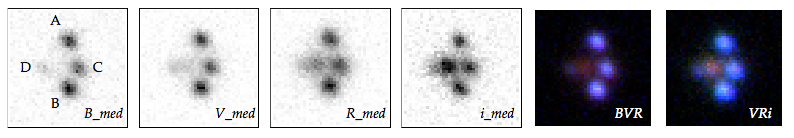
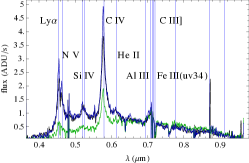
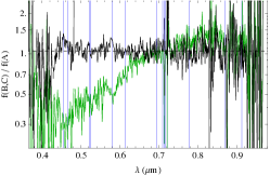
Figure 1: J1433+6007 discovery and follow-up data. Top: ALFOSC $BVRi$ median coadds and colour-composites, $0.21^{{\prime\prime}}$/px, North up and East left. A faint arc, barely visible in $B-$band, emanates from the northern-most image. Bottom: North-South (left) and East-West spectra (center), and flux-ratios of spectra in North-South slit (right). Image C leaks in the North-South slit and is significantly reddened (right, green line), whereas images A,B have almost indistinguishable spectra (right, black line). The source has $z_{s}=2.74,$ as evaluated from C iv, where the wavelength calibration is most accurate.

Here, we report on the discovery and follow-up of a quadruply lensed quasar, J1433+6007, mined with a novel technique in the Sloan Digital Sky Survey (SDSS, Abazajian et al., 2009) DR12 footprint without spectroscopic or UVx information. The two brightest images are separated by $\approx 3.6^{{\prime\prime}},$ the source redshift from the discovery spectra is $z_{s}=2.74,$ and the lens redshift is $z_{l}=0.407$ from follow-up Keck-ESI spectroscopy. We describe the target/candidate selection procedure in Section 2, the confirmation and follow-up of J1433 in Sect. 3, and first lens models in Sect. 4. We conclude in Section 5. In what follows, SDSS magnitudes are in the AB system, WISE (Wright et al., 2010) magnitudes in the Vega system, and where necessary we adopt concordance cosmological parameters $\Omega_{\Lambda}=0.7,$ $\Omega_{m}=0.3,$ $H_{0}=70$km/s/Mpc.

2 Candidate Selection

Since half of the known quasar lenses in SDSS have extended morphology, due to the presence of the deflector (see Williams et al., 2017, for a discussion), objects with $\log_{10}\mathcal{L}_{star,i}<-11$ or psf_i-mod_i$>$0.075, mod_i$<20.5,$ and WISE $W1-W2>0.55,$ $W2-W3<3.1+1.5(W1-W2-1.075)$ were pre-selected. Minimal $griz$ cuts were used. The $i-$band selection is used as a morphological preselection, whereas the WISE cuts are an extension of those by Assef et al. (2013) to exclude most quasars at $z<0.35$ and narrow-line galaxies. Quasar lens targets were then selected based on their catalog magnitudes, then visually inspected to exclude obvious contaminants, yielding the final candidate sample.

Lensed quasars are rare among quasars, which in turn are rarer than blue galaxies, hence we used a novel outlier selection to mine targets (detailed elsewhere, Agnello 2017), retaining peculiar objects by excluding more common ones. When tested on the SQLS morphologically-selected lens candidates of Inada et al. (2012), this procedure recovered 9 of the 10 lenses and excluded half of the 40 false positives, without any UVx or fibre-spectroscopy information.

Four classes of ‘common’ objects were defined, roughly corresponding to nearby ($z<0.75$) quasars, isolated quasars at higher ($z\approx 2$) redshift, blue-cloud galaxies and faint ($W2\gtrsim 15$) objects. Each class $k$ was represented by a single Gaussian with mean $\boldsymbol{\mu}_{k}$ and covariance $\mathbf{C}_{k}$ in a space given by $g-r,$ $g-i,$ $r-z,$ $i-W1,$ $W1-W2,$ $W2-W3,$ $W2$ and each object $\mathbf{f}$ was assigned pseudo-distances defined as $d_{k}=0.5\left\langle\mathbf{f}-\boldsymbol{\mu}_{k},\mathbf{C}_{k}^{-1}(\mathbf{f}-\boldsymbol{\mu}_{k})\right\rangle.$ Objects that were ‘far’ enough from the four class centers, based on linear combinations of their $d_{k}$ values, were retained as targets.

This yielded $\approx 250$ candidates brighter than $i=20.0$ over the whole SDSS-DR12 footprint, of which $\approx 40$ known quasar lenses or pairs. J1433+6007, at r.a.= 14:33:22.8, dec.=+60:07:13.44 (J2000), showed two well-separated blue images on either sides of two red objects, blended in three photometric components by the SDSS pipeline.

img.	$\delta x(^{\prime\prime})$	$\delta y(^{\prime\prime})$	$B$	$V$	$R$	$i$	$\mu$	$t-t_{A}$
	$=-\cos(\mathrm{dec.})\delta\mathrm{r.a.}$	$=\delta\mathrm{dec.}$	(mag)	(mag)	(mag)	(mag)		(days)
A	$0.00\pm 0.025$	$0.00\pm 0.025$	$20.26\pm 0.04$	$19.78\pm 0.01$	$19.26\pm 0.01$	$19.32\pm 0.01$	$2.62$	0.00
B	$-0.070\pm 0.025$	$-3.650\pm 0.025$	$20.09\pm 0.03$	$19.63\pm 0.01$	$19.13\pm 0.01$	$19.10\pm 0.01$	$3.57$	15.0
C	$0.766\pm 0.025$	$-2.056\pm 0.025$	$20.50\pm 0.05$	$19.92\pm 0.01$	$19.30\pm 0.01$	$19.14\pm 0.01$	$-3.07$	25.0
D	$-2.138\pm 0.050$	$-2.132\pm 0.050$	$22.00\pm 0.14$	$21.30\pm 0.02$	$20.63\pm 0.02$	$20.38\pm 0.01$	$-0.62$	113.0
G	$-1.152\pm 0.025$	$-1.950\pm 0.025$	$21.87\pm 0.15$	$20.69\pm 0.12$	$19.39\pm 0.01$	$18.52\pm 0.01$	—	—

Table 1: Image positions, $BVRi$ magnitudes, and model-predicted values of magnifications and time-delays. The nominal errors on some magnitudes would be smaller than quoted, but are limited by the accuracy of the ALFOSC zero-points and observing sky conditions.

3 Follow-up

Long-slit discovery spectra were obtained on 2017/01/19,20 as part of a candidate lens follow-up program (P42-019, PI Grillo). We used the Andalucia Faint Object Spectrograph and Camera (ALFOSC) at the 2.5m Nordic Optical Telescope (NOT) in La Palma (Spain), and the $1^{\prime\prime}-$wide long-slit with the #4 grism, covering a wavelength range $3200\rm{\AA}<\lambda<9600\rm{\AA}$ with a dispersion of $3.3\rm{\AA}/\rm{pixel}$. Standard Iraf routines were used for bias subtraction, flat-field corrections and wavelength calibration. From ALFOSC $BVRi$ imaging, we obtained the positions and magnitudes subsequently used for lens models. Deeper, high-resolution spectroscopy was obtained with the Echellette Spectrograph and Imager (ESI) at the Keck II telescope on 2017/01/20 (PI Jones), with a $1^{\prime\prime}$-wide slit, and reduced with ESIRedux.

In what follows, quasar images are labeled as shown in Fig 1, top-left, along the expected arrival times. ALFOSC pixels measure $0.21^{{\prime\prime}}$ per side.

3.1 NOT discovery and follow-up spectra

We took two 600s exposures with the slit aligned North-South, through 14:33:22.8+60:07:13.44, and one (900s) with East-West alignment, through 14:33:22.8+60:07:14.5. This enabled simultaneous spectroscopy of the two prominent quasar images and the two red objects, respectively. Arc (HeNe, Ar) and flat lamps were used for calibrations.

The North-South spectra show three nearly identical traces corresponding to the same $z_{s}=2.74$ quasar (Fig. 1, lower-left panel). The bright, outer traces correspond to the blue images (A,B) visible in the SDSS. The central, fainter trace is given by a third quasar image C, corresponding to the West-most red object, just outside the slit, thus confirming J1433 as a multiply imaged quasar. The East-West spectra (Fig. 1, lower-middle panel) show clear traces corresponding to images C,D and the lens galaxy (G). Images A,B have almost indistinguishable spectra, with uniform flux ratio $\approx 1.05,$ whereas image C undergoes substantial extinction bluewards of C iii$\left.\right]$. Micro-lensing results in $\approx 5-10\%$ flux-ratio differences between the continua and emission lines (Fig. 1, lower-right panel).

3.2 NOT imaging

Follow-up imaging data with good seeing ($\approx 0.6^{{\prime\prime}}$ FWHM at Zenith) were obtained with ALFOSC in $B,$ $V,$ $R,$ $i$ bands, using multiple $60$s exposures per band. Standard Python routines were used for bias subtraction, flat-fielding and coadding. The median coadds and colour-composites are shown in Fig. 1, where Ly $\alpha$ from the quasar images dominates in $B-$band and the lens brightens up in redder bands.

The relative displacements are obtained both from imaging and spectroscopic data. Individual traces in the spectra are well described by Gaussians in the spatial direction, whose run with wavelength can be modeled with uncertainties as low as 0.125px$=25$mas. Uncertainties from imaging-only data, though nominally smaller, are dominated by systematics from different noise realizations. Residuals between imaging data and model, mostly due to faint features and PSF mismatch, are within the noise level.

Table 1 gives the positions of the four images (A,B,C,D) and deflector (G), relative to image A, and $BVRi$ magnitudes. Images C and D are substantially reddened, and blending between D and G is significant in $B-$band.

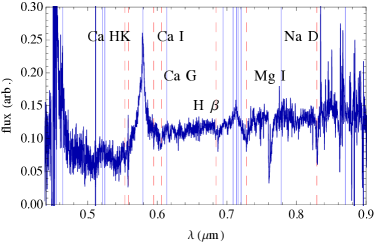
Figure 2: ESI follow-up spectra, with prominent absorption features at $z_{l}=0.407,$ which we associate with G. Red dashed lines: Ca HK, G-band $\lambda$4304, Mg i, Na D absorption at $z_{l}$. Blue solid lines: quasar emission at $z_{s}$. The Ca HK complex is visible, albeit at lower S/N, also in the ALFOSC spectra.

3.3 Keck-ESI follow-up

ESI spectra of G were taken in echellette mode, with $1.0^{{\prime\prime}}$ slit-width oriented East-West. The total integration time was 45 minutes split into 3 exposures of 900 seconds each. The combined 1D spectrum of G and D, shown in Figure 2, has distinctive absorption features at $z_{l}=0.407$ (Ca HK, G-band, H$\beta,$ Mg i/Fe complex, Na D), which we associate with the lens galaxy. The same features could be seen in the ALFOSC discovery spectra, though not as clear.

	$\theta_{\rm E}$	$q$	$\phi_{l}$	$\phi_{\rm s}$	$\gamma_{\rm s}$
best	1.80′′	0.50	0.18[rad]	1.12[rad]	0.10
68% low	1.70′′	0.43	0.13[rad]	0.96[rad]	0.08
68% high	1.90′′	0.58	0.25[rad]	1.22[rad]	0.13

Table 2: Lens model parameters: best-fit (first column) and 68% confidence intervals, marginalized over other parameters. Tight (and expected) degeneracies among parameters are present, given in eq. (2), except for the combination $\theta_{\rm E},$ which corresponds to the Einstein radius. Angles $\phi_{l},\phi_{\rm s}$ are positive counter-clockwise from West.

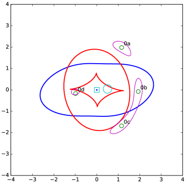
Figure 3: Lens model results: input images (green circles) and lens center (cyan square), $0.2^{\prime\prime}-$radius circle around the inferred source position (cyan), critical curve (blue) and radial and astroid caustics (red). Purple lines show isophotes corresponding to the source-plane contour. The position of image D is slightly biased, due to blending with G, but is recovered within the adopted uncertainties.

4 Lens models

From the relative displacements in Table 1, we fit a simple lens model to obtain the enclosed (2D) mass and predicted magnifications and time-delays. We do a conjugate-point analysis using Glee (Suyu & Halkola, 2010; Suyu et al., 2012), adopting $25$mas uncertainties on the positions of A,B,C and G, and $50$mas uncertainties on the position of image D. The surface density of the lens is described by

$$\kappa(x,y)=\frac{\Sigma(x,y)}{\Sigma_{\rm cr}}=\frac{b}{2\sqrt{X^{2}/(1+e)^{2}\,+Y^{2}/(1-e)^{2}}}$$ (1)

(Kassiola & Kovner, 1993), along the principal axes $(X,Y)$ of G, where $\Sigma_{\rm cr}=\mathrm{c}^{2}D_{s}/(4\pi G\,D_{l}D_{ls})$ factors the dependence on angular-diameter distances. The Einstein radius is defined as the geometric mean of the major and minor axes of the critical curve, $\theta_{\rm E}=2b\sqrt{q}/(1+q).$ We include external shear, with amplitude $\gamma_{\rm s}$ and angle $\phi_{\rm s},$ and let all parameters free to vary, including the lens flattening $q=(1-e)/(1+e)$ and position angle $\phi_{l}.$

The results are summarized in Tables 1,2 and Figure 3. The Einstein radius is robustly determined to $\theta_{\rm E}=(1.80\pm 0.10)^{\prime\prime}$, very close to half the A-B separation and independent of other inferred quantities. Flux-ratios from the best-fit model are comparable to those measured in $i-$band, accounting for differential extinction whose existence in lensing is well established (e.g. Falco et al., 1999; Mediavilla et al., 2005; Agnello et al., 2017). The predicted delays $t_{D}-t_{A}>100$d, $t_{C}-t_{A}\approx 25$d can be accurately measured in one or two seasons of high-cadence monitoring.

Monopole-quadrupole degeneracies (e.g. Kochanek, 2006) are present, in particular

$$\gamma_{\rm s} \approx 0.10+0.35(q-0.5),$$

$$\phi_{\rm s} \approx 1.1-1.5(b-2.5),$$

$$\gamma_{\rm s} \approx 0.10+0.35(\phi_{l}-0.8)$$ (2)

for this system. These may be broken with: observations of the line-of-sight environment, to characterize external contributions to the deflections; and higher-resolution imaging, of both the lensed quasar host and of G, to disentangle shear and lens flattening.

The velocity dispersion $\sigma$ of stars in the lens is a useful observable that can be estimated from the lens model itself. In fact, a direct measurement of $\sigma$ and its comparison with predictions from lensing can be used to measure cosmological distances and to constrain the dark matter density profile of the lens (Treu & Koopmans, 2004; Grillo et al., 2008; Paraficz & Hjorth, 2009; Suyu et al., 2014; Sonnenfeld et al., 2015; Jee et al., 2016). In the Singular Isothermal Sphere (SIS) limit $q\rightarrow 1,$ $\sigma$ depends weakly on location  and is well approximated by

$$\sigma_{\rm sis}^{2}=\frac{\mathrm{c}^{2}\theta_{\rm E}D_{s}}{4\pi D_{ls}}\ .$$ (3)

With the above values, we then obtain $\sigma=(290\pm 8)$ km/s, as expected for massive ellipticals (Treu et al., 2005). A direct comparison between the estimate in eq. (3) and direct measurements will need dynamical models that encompass asphericity and inclination effects (Barnabè et al., 2011).

5 Discussion and Conclusions

We have found a new, quadruply lensed quasar at RA= 14:33:22.8, DEC=+60:07:14.5, via an outlier-selection procedure applied to the SDSS-DR12 photometric footprint. Similar to other recent, wide-field photometric searches, this search did not rely on previous spectroscopic or UV excess information. This approach enables the discovery of systems with sources at higher redshifts than typically probed, and with appreciable differential reddening by the lens galaxy, similar to the recently discovered DES J0408-5354 (Lin et al., 2017; Agnello et al., 2017).

Discovery NOT-ALFOSC data confirmed this system as a lens with $z_{s}=2.74$ and four images on a fold configuration. The lens redshift is $z_{l}=0.407$ from follow-up Keck-ESI spectroscopy, which together with the lens model results with $\theta_{\rm E}=(1.80\pm 0.10)^{{\prime\prime}}$ predicts a velocity dispersion $\sigma=(290\pm 9)$km/s. Saddle-point images C,D are significantly reddened by the lens galaxy, while the A/B flux ratios agree with predictions by the lens model within $\approx 0.1$mag. Microlensing is evident in the differential magnification of lines and continua. The expected time-delays (tab. 1) can be measured accurately with high-cadence campaigns spanning one or two monitoring seasons. With current data, significant monopole-quadrupole degeneracies arise in the lens model, but they can be broken with deeper and higher-resolution follow-up.

References

- Abazajian et al. (2009) Abazajian, K. N., Adelman-McCarthy, J. K., Agüeros, M. A., et al. 2009, ApJS, 182, 543
- Agnello et al. (2013) Agnello, A., Auger, M. W., & Evans, N. W. 2013, MNRAS, 429, L35
- Agnello et al. (2015a) Agnello, A., Kelly, B. C., Treu, T., & Marshall, P. J. 2015, MNRAS, 448, 1446
- Agnello et al. (2016) Agnello, A., Sonnenfeld, A., Suyu, S. H., et al. 2016, MNRAS, 458, 3830
- Agnello et al. (2017) Agnello, A., Lin, H., Buckley-Geer, L., et al. 2017, MNRAS sumb. arXiv:1702.00406
- Assef et al. (2013) Assef, R. J., Stern, D., Kochanek, C. S., et al. 2013, ApJ, 772, 26
- Barnabè et al. (2011) Barnabè, M., Czoske, O., Koopmans, L. V. E., Treu, T., & Bolton, A. S. 2011, MNRAS, 415, 2215
- Braibant et al. (2016) Braibant, L., Hutsemékers, D., Sluse, D., & Anguita, T. 2016, AA, 592, A23
- Chan et al. (2015) Chan, J. H. H., Suyu, S. H., Chiueh, T., et al. 2015, ApJ, 807, 138
- Dalal & Kochanek (2002) Dalal, N., & Kochanek, C. S. 2002, ApJ, 572, 25
- Ding et al. (2017) Ding, X., Liao, K., Treu, T., et al. 2017, MNRAS, 465, 4634
- Falco et al. (1999) Falco, E. E., Impey, C. D., Kochanek, C. S., et al. 1999, ApJ, 523, 617
- Grillo et al. (2008) Grillo, C., Lombardi, M., & Bertin, G. 2008, AA, 477, 397
- Grillo et al. (2015) Grillo, C., Suyu, S. H., Rosati, P., et al. 2015, ApJ, 800, 38
- Inada et al. (2012) Inada, N., Oguri, M., Shin, M.-S., et al. 2012, AJ, 143, 119
- Jee et al. (2016) Jee, I., Komatsu, E., Suyu, S. H., & Huterer, D. 2016, JCAP, 4, 031
- Kassiola & Kovner (1993) Kassiola, A., & Kovner, I. 1993, Liege International Astrophysical Colloquia, 31, 571
- Kochanek (2006) Kochanek, C. S. 2006, Saas-Fee Advanced Course 33: Gravitational Lensing: Strong, Weak and Micro, 91
- Lin et al. (2017) Lin, H., Buckley-Geer, E., Agnello, A., et al. 2017, ApJL subm., arXiv:1702.00072
- Mediavilla et al. (2005) Mediavilla, E., Muñoz, J. A., Kochanek, C. S., et al. 2005, ApJ, 619, 749
- More et al. (2016) More, A., Lee, C.-H., Oguri, M., et al. 2016, arXiv:1608.06288
- Nierenberg et al. (2014) Nierenberg, A. M., Treu, T., Wright, S. A., Fassnacht, C. D., & Auger, M. W. 2014, MNRAS, 442, 2434
- Oguri et al. (2006) Oguri, M., Inada, N., Pindor, B., et al. 2006, AJ, 132, 999
- Oguri & Marshall (2010) Oguri, M., & Marshall, P. J. 2010, MNRAS, 405, 2579
- Ostrovski et al. (2017) Ostrovski, F., McMahon, R. G., Connolly, A. J., et al. 2017, MNRAS, 465, 4325
- Paraficz & Hjorth (2009) Paraficz, D., & Hjorth, J. 2009, AA, 507, L49
- Refsdal (1964) Refsdal, S. 1964, MNRAS, 128, 307
- Rusu et al. (2014) Rusu, C. E., Oguri, M., Minowa, Y., et al. 2014, MNRAS, 444, 2561
- Schechter et al. (2014) Schechter, P. L., Pooley, D., Blackburne, J. A., & Wambsganss, J. 2014, ApJ, 793, 96
- Schechter et al. (2016) Schechter, P. L., Morgan, N. D., Chehade, B., et al. 2016, arXiv:1607.07476
- Sonnenfeld et al. (2015) Sonnenfeld, A., Treu, T., Marshall, P. J., et al. 2015, ApJ, 800, 94
- Suyu & Halkola (2010) Suyu, S. H., & Halkola, A. 2010, AA, 524, A94
- Suyu et al. (2012) Suyu, S. H., Hensel, S. W., McKean, J. P., et al. 2012, ApJ, 750, 10
- Suyu et al. (2014) Suyu, S. H., Treu, T., Hilbert, S., et al. 2014, ApJL, 788, L35
- Treu & Koopmans (2004) Treu, T., & Koopmans, L. V. E. 2004, ApJ, 611, 739
- Treu et al. (2005) Treu, T., Ellis, R. S., Liao, T. X., et al. 2005, ApJ, 633, 174
- Williams et al. (2017) Williams, P., Agnello, A., & Treu, T. 2017, MNRAS, 466, 3088
- Wright et al. (2010) Wright, E. L., Eisenhardt, P. R. M., Mainzer, A. K., et al. 2010, AJ, 140, 1868-1881