Constraints on QSO emissivity using H i and He ii Lyman alpha forest

Abstract

The spectrum of cosmic ultraviolet background radiation at He ii ionizing energies ($\rm E\geq 4\,Ryd$) is important to study the He ii reionization, thermal history of the intergalactic medium (IGM) and metal lines observed in QSO absorption spectra. It is determined by the emissivity of QSOs at $\rm E\geq 4\,Ryd$ obtained from their observed luminosity functions and the mean spectral energy distribution (SED). The SED is approximated as a power-law at energies $\rm E\geq 1$ Ryd, $f_{E}\propto\rm E^{\alpha}$, where the existing observations constrain the power-law index $\alpha$ only up to $\sim$ 2.3 Ryd. Here, we constrain $\alpha$ for $\rm E\geq 4\,Ryd$ using recently measured He ii Lyman-$\alpha$ effective optical depths ($\tau_{\rm\alpha}^{\rm He\,II}$), H i photoionization rates and updated H i distribution in the IGM. We find that $-1.6>\alpha>-2$ is required to reproduce the $\tau_{\rm\alpha}^{\rm He\,II}$ measurements when we use QSO emissivity obtained from their luminosity function using optical surveys. We also find that the models where QSOs can alone reionize H i can not reproduce the $\tau_{\rm\alpha}^{\rm He\,II}$ measurements. These models need modifications, such as a break in mean QSO SED at energies greater than 4 Ryd. Even after such modifications the predicted He ii reionization history, showing that the He ii is highly ionized even at $z\sim 5$, is significantly different from the standard models. Therefore, the thermal history of the IGM will be crucial to distinguish these models. We also provide the He ii photoionization rates obtained from binned $\tau_{\rm\alpha}^{\rm He\,II}$ measurements.

1 Introduction

The observed ionization state of the intergalactic medium (IGM) at $z\leq 6$ (Gunn & Peterson, 1965; Fan et al., 2006; Becker & Bolton, 2013) is maintained by cosmic ultraviolet background (UVB) radiation emanating from Quasi-stellar Objects (QSOs) and galaxies (Miralda-Escude & Ostriker, 1990; Shapiro et al., 1994; Haardt & Madau, 1996; Shull et al., 1999). Apart from being the main driver of the hydrogen and helium reionization, the UVB maintains the ionization state of metals in the IGM and in the circum-galactic environments of galaxies. Therefore, the spectrum of UVB is important to study the cosmic metal mass density and the metal enrichment of the IGM (see for e.g.; Songaila & Cowie, 1996; Songaila, 2001; Carswell et al., 2002; Bergeron et al., 2002; Simcoe et al., 2004; Shull et al., 2014; Peeples et al., 2014; Hussain et al., 2017) by relating the observed ionic abundances to metal abundances.

Table 1: Measurements of the power-law index $\alpha$ (where $f_{\nu}\propto\nu^{\alpha}$)

Reference	$\alpha$	$\lambda_{\rm rest}$-Range	NQSOs	$z$-Range	Survey
(1)	(2)	(3)	(4)	(5)	(6)
Telfer et al. (2002)	-1.57$\pm$0.17	$500-1200$Å	77	$>0.33$	HST/FOS (radio-quite sample)
Telfer et al. (2002)	-1.96$\pm$0.12	$500-1200$Å	107	$>0.33$	HST/FOS (radio-loud sample)
Scott et al. (2004)	-0.56$\pm$0.38	$630-1150$Å	85	$<0.67$	FUSE
Shull et al. (2012a)	-1.41$\pm$0.21	$550-1000$Å	15	$0.45-1.44$	HST/COS
Stevans et al. (2014)	-1.41$\pm$0.15	$500-1000$Å	159	$<1.476$	HST/COS
Lusso et al. (2015)	-1.70$\pm$0.61	$600-912$Å	53	$2.3-2.6$	HST/WFC3
Tilton et al. (2016)	-0.72$\pm$0.26	$425-850$Å	20	$1.0-2.1$	HST/COS

Notes:
Column (1) gives references. Column (2) provides the measurements of $\alpha$ with the quoted 1-$\sigma$ errors measured for the rest wavelength ($\lambda_{\rm rest}$) range as given in column (3). Column (4) shows the number of QSOs (N_QSOs) used to obtain the composite spectrum having emission redshift as given in column (5). Column (6) provides information about survey, i.e the instrument, telescope and sample characteristics, where FOS stands for the Faint Object Spectrograph and WFC3 stands for the Wide Field Camera 3 on board HST.

Spectrum of the UVB depends on the spectral energy distribution (SED) of the sources that are contributing to it, mainly QSOs and star-forming galaxies. If we divide the UVB naively into hydrogen ionizing part (1 Ryd$<\rm E<$4 Ryd) and helium ionizing part ($\rm E\geq 4$ Ryd), the former is contributed by both galaxies and QSOs but latter is predominantly contributed by only QSOs. The relative contribution by QSOs and galaxies to the hydrogen ionizing part of the UVB depends on average escape fraction ($f_{\rm esc}$), a parameter that quantifies the amount of hydrogen ionizing photons escaping from galaxies. The $f_{\rm esc}(z)$ can be obtained using the measurements of hydrogen photoionization rates ($\Gamma_{\rm HI}$) for a given QSO emissivity and star formation history of galaxies (see Inoue et al., 2006; Khaire et al., 2016). On the other hand, for the measured $\Gamma_{\rm HI}(z)$ and the H i distribution in the IGM, the helium ionizing part of the UVB depends only on the QSO emissivity at $\rm E\geq 4$ Ryd. This emissivity is estimated through QSO luminosity functions and the mean SED of QSOs. The SED is usually approximated as a power-law, $f_{\nu}\propto\nu^{\alpha}$ at $\rm E\geq 1$ Ryd ($\lambda\leq 912$Å) from the observed composite QSO spectra (Zheng et al., 1997; Telfer et al., 2002; Scott et al., 2004; Stevans et al., 2014; Lusso et al., 2015). Although the existing observations have probed mean QSO SED only up to E$\sim$2.3 Ryd ($\lambda\sim 400$Å), it is usually extrapolated up to 35 Ryd ($\lambda\sim 25$Å) to calculate the He ii ionizing emissivity and the UVB. The reported values of the power-law index $\alpha$ show large variation from $-0.56$ to $-1.96$. Moreover, the number of QSOs where SED at high-energies can be directly probed is very small (see for e.g., Tilton et al., 2016). The existing measurements of $\alpha$ over the last two decades are summarized in Table 1. Using different $\alpha$ in UVB models gives significantly different UVB spectrum especially for $\rm E\geq 4$ Ryd. Also, the He ii ionizing emissivities obtained using different $\alpha$ provide different histories of the He ii reionization. Like hydrogen ionizing part of the UVB, we need measurements of He ii photoionization rates ($\Gamma_{\rm HeII}$) that can be used to constrain the He ii ionizing emissivity. The accurate estimate of UVB spectrum, especially at ${\rm E}\geq 4$ Ryd ($\lambda\leq 228$Å), is important for studying the ionization mechanism for high ionization systems such as O vi (see for e.g Danforth & Shull, 2005; Tripp et al., 2008; Muzahid et al., 2012; Pachat et al., 2016) and Ne viii (see for e.g.; Savage et al., 2005, 2011; Narayanan et al., 2012; Meiring et al., 2013; Hussain et al., 2015, 2017) which are believed to trace the warm-hot phase of the IGM. It is also important for studying the thermal history of the IGM (Lidz et al., 2010; Bolton et al., 2010; Becker et al., 2011; Bolton et al., 2012; Khrykin et al., 2017) and the process of He ii reionization (Faucher-Giguère et al., 2009; McQuinn et al., 2009; Compostella et al., 2013; La Plante & Trac, 2016). The above mentioned importance of $\alpha$ and the issues with its measurements motivate us to theoretically constrain $\alpha$ at ${\rm E\geq 4}$ Ryd. For that we use the observations of H i and He ii Lyman-$\alpha$ forest.

The He ii Lyman-$\alpha$ forest has been observed for few QSOs at $z>2.5$ with UV spectrographs on space telescopes such as Far Ultraviolet Spectroscopic Explorer (FUSE; Kriss et al., 2001; Shull et al., 2004; Fechner et al., 2006) and Cosmic Origin Spectrograph (COS) on-board Hubble Space Telescopes (HST; Syphers et al., 2011; Worseck et al., 2016). With such observations the Lyman-$\alpha$ effective optical depths of He ii ($\tau_{\rm\alpha}^{\rm He\,II}$; Shull et al., 2010; Syphers & Shull, 2013; Worseck et al., 2011) and the ratio of He ii to H i in the IGM absorbers (Zheng et al., 2004; Muzahid et al., 2011; McQuinn & Worseck, 2014) have been measured. The recent measurements of $\tau_{\rm\alpha}^{\rm He\,II}$ by Worseck et al. (2016) at $2.3<z<3.5$ can be used to constrain the He ii ionizing emissivity and the properties of QSO SED such as the spectral index $\alpha$. This is what we explore in our analysis.

For a given QSO emissivity at $1$ Ryd and a mean SED of QSOs, using our cosmological radiative transfer code (Khaire & Srianand, 2013, 2015b, 2015a), we estimate the He ii ionizing UVB, photoionization rates of He ii and $\tau_{\rm\alpha}^{\rm He\,II}$. We also calculate the corresponding He ii reionization history. By comparing these values with the $\tau_{\rm\alpha}^{\rm He\,II}$ measurements, we constrain the mean SED of QSOs. We use two models of QSO emissivity, one obtained from the compilation of optically selected QSOs (Khaire & Srianand, 2015a) and the other where QSOs can alone reionize H i when extrapolated to $z>6$ (Madau & Haardt, 2015; Khaire et al., 2016). The latter uses the QSO luminosity function of Giallongo et al. (2015) that claimed to detect large number density of low luminosity QSOs at $z>4$. Using $\tau_{\rm\alpha}^{\rm He\,II}$ and $\Gamma_{\rm HI}$ measurements we also estimate the $\Gamma_{\rm HeII}$ values that depends only on the H i distribution of the IGM and independent of the UVB models.

The paper is organized as follows. In section 2, we discuss the basic theory to calculate $\tau_{\rm\alpha}^{\rm He\,II}$ using H i distribution of the IGM and $\Gamma_{\rm HeII}$ using $\tau_{\rm\alpha}^{\rm He\,II}$ measurements. In Section 3, we explain the basic theory and assumptions to calculate the He ii ionizing emissivity, the UVB and the He ii reionization history. In Section 4, we discuss our results for different models of QSO emissivity and uncertainties. We present the summary in section 5. Throughout this paper we use cosmology parameters $\Omega_{\Lambda}=0.7$, $\Omega_{m}=0.3$ and $H_{0}=70$ km s^-1 Mpc^-1 consistent with that from Planck Collaboration et al. (2016).

2 He ii optical depths and photoionization rates

2.1 Basic theory: Lyman-$\alpha$ effective optical depths

The Lyman-$\alpha$ effective optical depth for H i ($\tau_{\rm\alpha}^{\rm H\,I}$) and He ii ($\tau_{\rm\alpha}^{\rm He\,II}$) at redshift $z$ is obtained by (Paresce et al., 1980; Madau & Meiksin, 1994),

$$\tau_{\alpha}^{x}(z)=\frac{1+z}{\lambda^{{}^{x}}_{\alpha}}\int_{N^{\rm min}_{\rm HI}}^{\infty}dN_{\rm HI}\,\frac{\partial^{2}N}{\partial N_{\rm HI}\partial z}\,W_{\rm n}^{x}\,\,.$$ (1)

Here, $x$ denotes the species H i or He ii, $\lambda^{{}^{x}}_{\alpha}$ is the rest-frame Lyman-$\alpha$ line wavelength of species $x$ (i.e, 1215.67Å for H i and 303.78Å for He ii), $N_{\rm H\,I}^{\rm min}$ is the minimum column density of H i used in the integral and $\partial^{2}N/\partial N_{\rm HI}\partial z=f(N_{\rm HI},z)$ is the column density distribution of H i. Here, $W_{\rm n}^{x}$ is the equivalent width of the Lyman-$\alpha$ line expressed in wavelength units for species $x$ as given by,

$$W_{\rm n}^{x}=\int_{0}^{\infty}d\lambda\,[1-e^{-y\phi_{x}(\lambda)}]\,\,,$$ (2)

where, $\phi_{x}(\lambda)$ is the Voigt profile function for species $x$, $y=N_{\rm HI}$ when $x$ is H i and $y=\eta\times N_{\rm HI}$ when $x$ is He ii where $\eta=N_{\rm HeII}/N_{\rm HI}$.

The calculation of $\tau_{\rm\alpha}^{\rm H\,I}$ depends on the observed $f(N_{\rm HI},z)$. In the absence of the column density distribution of He ii, the calculation of $\tau_{\rm\alpha}^{\rm He\,II}$ relies on the the estimate of the parameter $\eta$. The $\eta$ determines the amount of $N_{\rm HeII}$ in intergalactic absorber having H i column density $N_{\rm HI}$. It is estimated under the assumption that the IGM is in photoionization equilibrium maintained by the UVB. The $\eta$ is independent of $N_{\rm HI}$ for the absorbers that are optically thin to He ii ionizing radiation ($N_{\rm HeII}\la 10^{16.8}{\rm cm^{-2}}$; obtained for continuum optical depth $\la 0.1$), called as $\eta_{\rm thin}$. The parameter $\eta_{\rm thin}$ is obtained from the relation,

$$\eta_{\rm thin}(z)=\frac{n_{\rm He}}{n_{\rm H}}\frac{\alpha^{A}_{\rm HeII}(\rm T)}{\alpha^{A}_{\rm HI}(\rm T)}\frac{\Gamma_{\rm HI}(z)}{\Gamma_{\rm HeII}(z)}.$$ (3)

Here, $\alpha^{A}_{x}(\rm T)$ and $\Gamma_{x}$ are the case A recombination rate coefficient (that depends on the gas temperature T) and the photoionization rate for species $x$, respectively, whilst $n_{\rm H}$ and $n_{\rm He}$ are the number density of total hydrogen and helium in the IGM, respectively. The ratio $n_{\rm He}/n_{\rm H}=y_{p}/(4-4y_{p})$ where $y_{p}$ is the primordial mass fraction of helium. Using $y_{p}=0.25$ from Planck Collaboration et al. (2016) and the expressions for recombination rate coefficients, Eq. 3 can be approximated as,

$$\eta_{\rm thin}(z)=0.45\Big{(}\frac{\rm T}{10^{4.3}{\rm K}}\Big{)}^{0.06}\frac{\Gamma_{\rm HI}(z)}{\Gamma_{\rm HeII}(z)}.$$ (4)

The above equation shows that $\eta_{\rm thin}$ weakly depends on the temperature and it is mainly decided by the ratio of $\Gamma_{\rm HI}$ to $\Gamma_{\rm HeII}$. Under photoionization equilibrium, $\eta$ at all $N_{\rm HI}$ obtained from radiative transfer simulations can be approximated by the following quadratic equation (Fardal et al., 1998; Faucher-Giguère et al., 2009; Haardt & Madau, 2012),

$$\frac{n_{\rm He}}{4n_{\rm H}}\,\frac{\Gamma_{\rm HI}}{n_{e}\alpha^{A}_{\rm HI}(\rm T)}\,\frac{\sigma_{912}N_{\rm HI}}{(1+{\rm A}\sigma_{912}N_{\rm HI})}=\sigma_{228}N_{\rm HeII}$$ (5)

$$\,+\,\frac{\Gamma_{\rm HeII}}{n_{e}\alpha^{A}_{\rm HeII}(\rm T)}\,\frac{\sigma_{\rm HeII}N_{\rm HeII}}{(1+{\rm B}\sigma_{228}N_{\rm HeII})}.$$

Here, $n_{e}$ is electron density, $\sigma_{228}$ is photoionization cross-section of He ii ($\sigma_{\rm HeII}$) at 228Å, $\sigma_{912}$ is photoionization cross-section of H i ($\sigma_{\rm HI}$) at 912Å, and A and B are the constants obtained by fitting numerical results. The above quadratic equation is supplemented by a relation between $n_{e}$ and $N_{\rm HI}$. We take this relation, $n_{e}=1.024\times 10^{-6}(N_{\rm HI}\Gamma_{\rm HI})^{(2/3)}{\rm cm^{-3}}$, T=20000K, and the values of $A=0.02$ and $B=0.25$ following Haardt & Madau (2012). These parameters are obtained for the clouds having plane parallel slab geometry and fixed line-of-sight length equal to the Jeans length following Schaye (2001). With the same set-up, we also verify these values using cloudy13 (Ferland et al., 2013). The $\eta$ obtained by solving Eq. 5 reduces to $\eta_{\rm thin}$ for optically thin clouds. Although we use Eq. 5 to calculate $\eta$ at all $N_{\rm HI}$, the $\tau_{\rm\alpha}^{\rm He\,II}$ is mainly due to optically thin clouds of He ii where $\eta=\eta_{\rm thin}$, therefore, $\tau_{\rm\alpha}^{\rm He\,II}$ is independent of the geometry or the finite size of clouds.

It is important to set the appropriate $N^{\rm min}_{\rm HI}$ in Eq. 1 since, $\tau^{x}_{\alpha}$ depends on it (see also Madau & Meiksin, 1994). It is because, for low column densities $W^{x}_{n}\propto N_{x}$ and the column density distribution of H i is a power-law in $N_{\rm HI}$, i.e, $f(N_{\rm HI},z)\propto N_{\rm HI}^{-\beta}$ where $\beta$ is a power-law index. Using these relations in Eq. 1 gives $\tau_{\rm\alpha}^{\rm H\,I}$ $\propto N^{2-\beta}_{\rm HI}$ and $\tau_{\rm\alpha}^{\rm He\,II}$ $\propto\eta_{\rm thin}N^{2-\beta}_{\rm HI}$. Therefore, it is unphysical to extrapolate the power-law $f(N_{\rm HI},z)$ to smaller $N_{\rm HI}$ than what observations suggest. We use the parametric form of $f(N_{\rm HI},z)$ from Inoue et al. (2014). It reproduces the observed redshift evolution of the $\tau_{\rm\alpha}^{\rm H\,I}$(z) (by Fan et al., 2006; Kirkman et al., 2007; Faucher-Giguère et al., 2008; Becker et al., 2013). Inoue et al. (2014) has used $N^{\rm min}_{\rm HI}=10^{12}\,{\rm cm^{-2}}$ and $b$-parameter (mean Doppler velocity to estimate the Voigt profile function) of 28 km $s^{-1}$ to calculate $\tau_{\rm\alpha}^{\rm H\,I}$ using Eq. 1. This corresponds to a minimum equivalent width of H i Lyman-$\alpha$ line to be $W_{n}^{\rm HI}=5.2\times 10^{-3}{\rm\AA}$. To calculate $\tau_{\rm\alpha}^{\rm He\,II}$, we use the same $b$-parameter assuming that the Doppler broadening is mostly dominated by turbulence and $N^{\rm min}_{\rm HI}=(16/\eta_{\rm thin})\times 10^{12}\,{\rm cm^{-2}}$ that gives the same minimum equivalent width for He ii as mentioned above for H i. In Section 4.3, we discuss the uncertainty in the obtained $\tau_{\rm\alpha}^{\rm He\,II}$ arising from these assumptions and its effect on the presented results.

In the following sub-section, we calculate $\eta_{\rm\,thin}$ from the $\tau_{\rm\alpha}^{\rm He\,II}$ measurements and estimate the corresponding He ii photoionization rates.

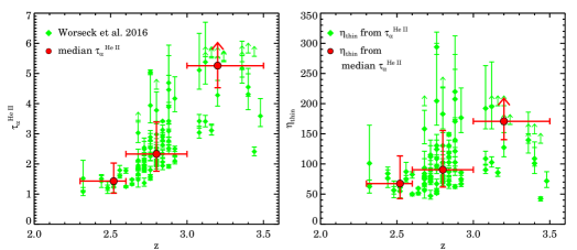
Figure 1: Left-hand panel: Measurements of $\tau_{\rm\alpha}^{\rm He\,II}$($z$) from Worseck et al. (2016). The red circles are the median $\tau_{\rm\alpha}^{\rm He\,II}$ in three redshift bins as given in Table 2. Horizontal bars show the sizes of redshift bins. Vertical error-bars on median $\tau_{\rm\alpha}^{\rm He\,II}$ show 95th percentile values of the distribution of errors in each redshift-bin. Right-hand panel: $\eta_{\rm\,thin}=N_{\rm HeII}/N_{\rm HI}$ calculated using the $\tau_{\rm\alpha}^{\rm He\,II}$ data as plotted on the left-hand panel. Red circles show the $\eta_{\rm\,thin}$ from the median $\tau_{\rm\alpha}^{\rm He\,II}$ data in three redshift bins as shown in the the left-hand panel. The values are provided in Table 2.

Table 2: $\Gamma_{\rm HeII}$ and $\lambda_{\rm mfp}$ estimates

Median $z$	2.52	2.8	3.2
$z$-range	$2.3-2.6$	$2.6-3.0$	$3.0-3.5$
amedian $\tau_{\rm\alpha}^{\rm He\,II}$	1.43${}^{+0.60}_{-0.40}$	2.33${}^{+1.06}_{-0.57}$	5.26${}^{+\infty}_{-0.73}$
$\eta_{\,\rm thin}$	67.4${}^{+45.9}_{-24.9}$	90.4${}^{+65.1}_{-28.7}$	170.8${}^{+\infty}_{-30.6}$
b$\Gamma_{\rm HI}$ in $10^{-12}$ s${}^{-1}~{}$	1.035${}^{+0.37}_{-0.30}$	0.86${}^{+0.30}_{-0.22}$	0.79${}^{+0.28}_{-0.19}$
$\Gamma_{\rm HeII}$ in $10^{-15}$ s-1	6.91${}^{+5.31}_{-3.22}$	4.28${}^{+3.42}_{-1.76}$	2.08${}^{+1.83}_{-\infty}$
$\lambda_{\rm mfp}$ in pMpc	32.9${}^{+10.7}_{-9.0}$	18.7${}^{+5.0}_{-5.4}$	7.5${}^{+1.0}_{-7.5}$

Notes:
^aErrors on the mean $\tau_{\rm\alpha}^{\rm He\,II}$  correspond to 95th percentile of the distribution of errors on $\tau_{\rm\alpha}^{\rm He\,II}$ measurements in the redshift-bin. ^b$\Gamma_{\rm HI}$ measurements from Becker & Bolton (2013).

2.2 He ii photoionization rates

In Eq. 1 and 2, the value of $\eta_{\,\rm thin}$ can be varied to obtain the desired value of $\tau_{\rm\alpha}^{\rm He\,II}$. By this method, one can obtain the values of $\eta_{\,\rm thin}$ for measured values of $\tau_{\rm\alpha}^{\rm He\,II}$. This $\eta_{\,\rm thin}$ along with the measurements of $\Gamma_{\rm HI}$ provides $\Gamma_{\rm HeII}$ (using Eq. 4). Here, we estimate $\eta_{\,\rm thin}$ using recent measurements of $\tau_{\rm\alpha}^{\rm He\,II}$ from Worseck et al. (2016). Then we calculate $\Gamma_{\rm HeII}$ using this $\eta_{\,\rm thin}$ and the $\Gamma_{\rm HI}$ measurements from Becker & Bolton (2013).

In the left-hand panel of Fig. 1 we show $\tau_{\rm\alpha}^{\rm He\,II}$ measurements of Worseck et al. (2016) which are calculated at redshift bin intervals of size 0.04 from HST-COS observations of 17 QSO sightlines having He ii Lyman-$\alpha$ forest. We calculate $\eta_{\,\rm thin}$ corresponding to each of these $\tau_{\rm\alpha}^{\rm He\,II}$ measurements. These are shown in the right-hand panel of Fig. 1. The error-bars on $\eta_{\rm thin}$ arise from 1-$\sigma$ errors on $\tau_{\rm\alpha}^{\rm He\,II}$. We need $\eta_{\rm thin}$ to have values in the range of 40 to 320 to reproduce the observed distribution of $\tau_{\rm\alpha}^{\rm He\,II}$. Note that, the $\eta_{\,\rm thin}$ calculated in this way ignores the differences in the $\tau_{\rm\alpha}^{\rm H\,I}$ one expects for different line-of sights. Although, the line-of-sight average $\tau_{\rm\alpha}^{\rm H\,I}$ at the regions where $\tau_{\rm\alpha}^{\rm He\,II}$ was measured show very good agreement with the mean $\tau_{\rm\alpha}^{\rm H\,I}$ (Faucher-Giguère et al., 2008; Becker et al., 2013, the same mean $\tau_{\rm\alpha}^{\rm H\,I}$ that has been used to obtain $f(N_{\rm HI},z)$ by Inoue et al. 2014), significant variations in $\tau_{\rm\alpha}^{\rm H\,I}$ occur on the $\Delta z=0.04$ scales (see figure 8 of Worseck et al., 2016).

To estimate $\Gamma_{\rm HeII}$, we need $\eta_{\,\rm thin}$ value in the same redshift range as the $\Gamma_{\rm HI}$ measurement. Therefore, we take median of the $\tau_{\rm\alpha}^{\rm He\,II}$ measurements in three redshift bins that are $z=2.3-2.6$, $z=2.6-3.0$ and $z=3.0-3.5$. These bins match closely with the redshift bins used for $\Gamma_{\rm HI}$ measurements by Becker & Bolton (2013). Here, instead of using mean redshift for bins, we use the median redshift since the distribution of $\tau_{\rm\alpha}^{\rm He\,II}$ in each bin is not uniform. The median $\tau_{\rm\alpha}^{\rm He\,II}$ values in these bins are shown in the left-hand panel of Fig. 1 and provided in the Table 2. The error-bars are the 95th percentile values of the distribution of errors in each bin. Since, the highest redshift-bin contains most of the lower limits on $\tau_{\rm\alpha}^{\rm He\,II}$ measurements, the median $\tau_{\rm\alpha}^{\rm He\,II}$ in this bin is also a lower limit. The $\eta_{\,\rm thin}$ values required to obtain these binned $\tau_{\rm\alpha}^{\rm He\,II}$ measurements are shown in the right-hand panel of Fig. 1 and provided in Table 2. Error-bars on $\eta_{\,\rm thin}$ are obtained from the error-bars on median $\tau_{\rm\alpha}^{\rm He\,II}$ as shown in the left-hand panel of Fig. 1. The median $\tau_{\rm\alpha}^{\rm He\,II}$ and $\eta_{\,\rm thin}$ show clear increasing trend with redshift. We obtain $\Gamma_{\rm HeII}$ for these $\eta_{\,\rm thin}$ values (from Eq. 4) using the $\Gamma_{\rm HI}$ measurements of Becker & Bolton (2013) in the corresponding redshift bins. Table 2 summarizes our estimated $\Gamma_{\rm HeII}$ values as well as the $\Gamma_{\rm HI}$ measurements that are used for obtaining them. The errors on $\Gamma_{\rm HeII}$ also account for the errors on $\Gamma_{\rm HI}$ measurements. Note that the $\Gamma_{\rm HeII}$ calculated in this way depends only on the $f(N_{\rm HI},z)$ and does not depend on the UVB models. Our $\Gamma_{\rm HeII}$ values are consistent with the values obtained by Worseck et al. (2016) using their semi-analytic model for post-reionization $\tau_{\rm\alpha}^{\rm He\,II}$. We have also calculated the mean free path for He ii ionizing photons ($\lambda_{\rm mfp}$; using Eq. 12 and 13 from Khaire & Srianand, 2013) that depends on $\eta$ and $f(N_{\rm HI},z)$, as given in Table 2 in units of proper Mpc. Errors on $\lambda_{\rm mfp}$ correspond to errors on the $\eta_{\rm thin}$ values.

In the next section, we discuss the implications of these inferred $\Gamma_{\rm HeII}$ and $\tau_{\rm\alpha}^{\rm He\,II}$ measurements for calculations of the UVB.

3 Helium ionizing UVB

We are interested in computing the He ii ionizing UVB to obtain $\Gamma_{\rm HeII}$ and $\tau_{\rm\alpha}^{\rm He\,II}$. This will be used in comparison with the $\tau_{\rm\alpha}^{\rm He\,II}$ measurements and the He ii reionization history to constrain the He ii ionizing QSO emissivity. In this section, we explain the basic theory to calculate the He ii ionizing UVB, the assumptions involved in estimating He ii ionizing emissivity and theory for calculating He ii reionization history.

3.1 The UVB

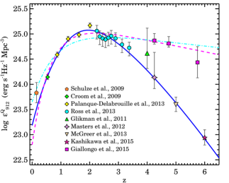
Figure 2: The QSO emissivity at $912$Å ($\epsilon^{Q}_{\nu_{912}}$) with $z$. Data points are taken from the compilations of Khaire & Srianand (2015a, see their Table 1) which used recent luminosity function of optically selected QSOs (Schulze et al., 2009; Croom et al., 2009; Glikman et al., 2011; Masters et al., 2012; Ross et al., 2013; Palanque-Delabrouille et al., 2013; McGreer et al., 2013; Kashikawa et al., 2015) and the emissivity from QSO luminosity function by Giallongo et al. (2015). Blue solid curve is a simple fit through the $\epsilon^{Q}_{\nu_{912}}$ obtained using optically selected QSOs (see Eq. 12; model A). Magenta dashed (model B1 from Eq. 13; Khaire et al., 2016) and cyan dot-dashed curve (model B2 from Eq. 14; MH15) are fits that include $\epsilon^{Q}_{\nu_{912}}$ from Giallongo et al. (2015) at $z>4$.

The photoionization rate, $\Gamma_{x}(z)$, at redshift $z$ for species $x$ is obtained by following integral,

$$\Gamma_{x}(z)=\int_{\nu_{x}}^{\infty}d\nu\,\frac{4\pi\,J_{\nu}(z)}{h\nu}\,\sigma_{x}(\nu)\,\,.$$ (6)

Here, $\nu_{x}$ ans $\sigma_{x}$ are the ionization threshold frequency and photoionization cross-section for the species $x$, respectively, $h$ is Planck constant and $J_{\nu}(z)$, in units of ergs cm^-2 s^-1 Hz^-1 sr^-1, is the angle averaged specific intensity of the UVB radiation at frequency $\nu$ and redshift $z$. $J_{\nu_{0}}(z_{0})$ is obtained by solving following cosmological radiative transfer equation (see Peebles, 1993; Haardt & Madau, 1996),

$$J_{\nu_{0}}(z_{0})=\frac{c}{4\pi}\int_{z_{0}}^{\infty}\,dz\frac{(1+z_{0})^{3}\,\epsilon_{\nu}(z)}{(1+z)H(z)}e^{-\tau_{\rm eff}(\nu_{0},z_{0},z)}.$$ (7)

Here, $c$ is the speed of light, $H(z)=H_{0}\sqrt{\Omega_{m}(1+z)^{3}+\Omega_{\Lambda}}$ is the Hubble parameter, frequency $\nu$ is related to $\nu_{0}$ by $\nu=\nu_{0}(1+z)/(1+z_{0})$, and $\epsilon_{\nu}(z)$ is the comoving emissivity of the sources. $\tau_{\rm eff}(\nu_{0},z_{0},z)$ is an effective optical depth encountered by a photon observed at $z_{0}$ having frequency $\nu_{0}$ while traveling from its emission redshift $z$ to $z_{0}$. Assuming that the IGM clouds along any line-of-sight are Poisson distributed, the $\tau_{\rm eff}$ is given by (see Paresce et al., 1980; Padmanabhan, 2002),

$$\tau_{\rm eff}(\nu_{0},z_{0},z)=\int_{z_{0}}^{z}dz^{\prime}\int_{N^{\rm min}_{\rm HI}}^{\infty}dN_{\rm HI}f(N_{\rm HI},z^{\prime})(1-e^{-\tau_{\nu^{\prime}}}).$$ (8)

Here, $\tau_{\nu^{\prime}}$ is the continuum optical depth encountered by photons emitted at frequency $\nu^{\prime}$ while traveling from their emission redshift $z^{\prime}$ to $z_{0}$. It is given by,

$$\tau_{\nu^{\prime}}=N_{\rm HI}{\sigma_{\rm HI}(\nu^{\prime})}+N_{\rm HeI}{\sigma_{\rm HeI}(\nu^{\prime})}+N_{\rm HeII}{\sigma_{\rm HeII}(\nu^{\prime})},$$ (9)

where, $\nu^{\prime}=\nu_{0}(1+z^{\prime})/(1+z_{0})$. In the redshift range of our interest ($z<4$) He i has negligible contribution to $\tau_{\nu^{\prime}}$ (see also Faucher-Giguère et al., 2009; Haardt & Madau, 2012). Therefore, we approximate $\tau_{\nu^{\prime}}$ as,

$$\tau_{\nu^{\prime}}=N_{\rm HI}[\,\sigma_{\rm HI}(\nu^{\prime})+\eta\,\sigma_{\rm HeII}(\nu^{\prime})\,]\,.$$ (10)

Note that, here the $\tau_{\rm eff}$ depends on $\eta(N_{\rm HI})$ and not just on $\eta_{\rm\,thin}$. The UVB is obtained by iteratively solving Eq. 5-10 for an assumed ionizing emissivity $\epsilon_{\nu}(z)$.

Here, we are interested in calculating the He ii ionizing UVB at $2<z<4$. For that, we need He ii ionizing emissivity (at $\lambda\leq 228$Å) and $\Gamma_{\rm HI}$ to estimate $\eta$. Since, we are using the measured values of $\Gamma_{\rm HI}$ at $z>2$, we do not need to explicitly calculate the H i ionizing UVB. However, note that, to calculate the He ii ionizing UVB at $z=z_{0}$ we need $\Gamma_{\rm HI}(z)$ at $z>z_{0}$. Therefore, in our UVB calculations, along with the $\Gamma_{\rm HI}$ measurements by Becker & Bolton (2013) at $2.4\leq z\leq 4.8$, we use $\Gamma_{\rm HI}$ at $z=2$ from Bolton & Haehnelt (2007) and at $z>5$ from Calverley et al. (2011) and Wyithe & Bolton (2011). We also estimate the UVB for 1-$\sigma$ higher and lower values of measured $\Gamma_{\rm HI}(z)$ to study the uncertainties arising in our results due to the uncertainties in the measured $\Gamma_{\rm HI}$.

The following subsection explains the usual procedure to estimate the He ii ionizing emissivity.

3.2 Helium ionizing emissivity

In the absence of population-iii stars at the redshifts of our interest, star-forming galaxies emit a negligible amount of He ii ionizing photons. Therefore, the helium ionizing emissivity $\epsilon_{\nu}$ at $\lambda\leq 228$Å is contributed by QSOs alone. Using the expression for QSO emissivity at 912Å ($\epsilon^{Q}_{912}$) and the mean SED of QSOs at $\lambda\leq 912$Å which is usually approximated as a power-law $f_{\nu}\propto\nu^{\alpha}$, the $\epsilon_{\nu}$ can be written as,

$$\epsilon_{\nu}(z)=\Big{(}\frac{\nu}{\nu_{912}}\Big{)}^{\alpha}\epsilon^{Q}_{\nu_{912}}(z),$$ (11)

where, $\nu_{912}=c/912$Å Hz.

Helium ionizing emissivity depends on $\epsilon^{Q}_{\nu_{912}}$ and $\alpha$. The $\epsilon^{Q}_{\nu_{912}}$ is obtained from QSO luminosity function along with the mean SED from optical to extreme UV wavelengths (up to $\sim 912$Å) that is well observed. However, at $\lambda\leq 912$Å, the power-law index $\alpha$ is measured only up to $\lambda\sim 425$Å (see Table 1). In absence of any observational constraints, this emissivity is usually extrapolated to smaller wavelengths (up to $\sim 25$Å) to estimate the He ii ionizing emissivity. Moreover, the values of $\alpha$ reported in the literature over last two decades are not consistent with each other. Reported values vary from -0.56 to -1.96 as summarized in the Table 1. The estimates of He ii ionizing UVB and the $\Gamma_{\rm HeII}$ are severely affected by the choice of $\alpha$ in the UVB models. These issues motivate us to constrain the $\alpha$ at $\lambda\leq 228$Å that is consistent with $\tau_{\rm\alpha}^{\rm He\,II}$ measurements and $\Gamma_{\rm HeII}$. For that, we use two models of $\epsilon^{Q}_{\nu_{912}}(z)$, namely model A and model B, as explained below:

• Model A: The model A uses the QSO luminosity functions observed at UV and optical wavebands at all redshifts as compiled in Khaire & Srianand (2015a, see their Table 1). To estimate the He ii ionizing emissivity and UVB, model A takes $\alpha$ as a free parameter and $\epsilon^{Q}_{\nu_{912}}(z)$ in units of ${\rm erg\,s^{-1}\,Hz^{-1}Mpc^{-3}}$ as (Khaire & Srianand, 2015a),

  $$\epsilon^{Q}_{\nu_{912}}(z)=10^{24.6}\,(1+z)^{5.9}\,\frac{\exp(-0.36z)}{\exp(2.2z)+25.1}\,\,.$$ (12)

  This is a simple fit through the compiled $\epsilon^{Q}_{\nu_{912}}$ values as shown in Fig. 2 (blue solid curve). This model needs additional contribution to H i ionizing photons from star-forming galaxies to reionize H i at $z>5.5$ and to be consistent with the $\Gamma_{\rm HI}$ measurements at $z>3$ (see Khaire et al., 2016).

• Model B: In addition to the QSO luminosity functions observed at UV and optical wavebands at $z<4$, model B uses the QSO luminosity function from Giallongo et al. (2015) at $z>4$ obtained by selecting QSO candidates based on their X-ray fluxes. In contrast with model A, model B do not require any contribution from star forming galaxies to reionize H i i.e QSOs alone reionize H i in this model (for e.g., Khaire et al., 2016; Madau & Haardt, 2015, hereafter MH15). Therefore, the H i ionizing emissivity obtained through choice of $\alpha$ and $\epsilon^{Q}_{\nu_{912}}(z)$ in model B has to simultaneously satisfy the observational constraints on H i reionization (Planck Collaboration et al., 2016; Schenker et al., 2014; McGreer et al., 2015) at $z>5.5$, unresolved X-ray background at $z>5$ (Moretti et al., 2012) and $\epsilon^{Q}_{\nu_{912}}$ obtained by Giallongo et al. (2015) at $z>4$. These constraints provide little room to change $\alpha$ for a given $\epsilon^{Q}_{\nu_{912}}(z)$ in model B. It is unlike the model A where the discrepancy in H i ionizing photons due to decreasing value of $\alpha$ can be resolved by increasing the contribution from star-forming galaxies. Therefore, instead of making $\alpha$ as a free parameter, for fixed value of $\alpha$ and corresponding $\epsilon^{Q}_{\nu_{912}}(z)$ we explore a break in QSO SED at He ii ionizing part (${\rm E}\geq 4$ Ryd) required to satisfy the $\tau_{\rm\alpha}^{\rm He\,II}$ measurements. In model B, we take two values of $\alpha$ and the corresponding two forms of $\epsilon^{Q}_{\nu_{912}}(z)$ that are shown to be consistent with the constraints mentioned above. First, we take $\alpha=-1.4$ (consistent with Stevans et al., 2014) and $\epsilon^{Q}_{\nu_{912}}(z)$ as

  $$\log\epsilon^{Q}_{\nu_{912}}(z)=25.35\exp(-0.0047z)-2.55\exp(-1.61z).$$ (13)

  This is consistent with the model presented in Khaire et al. (2016). We denote this combination of $\alpha$ and $\epsilon^{Q}_{\nu_{912}}(z)$ as model B1. Second, we take $\alpha=-1.7$ (consistent with Lusso et al., 2015) and $\epsilon^{Q}_{\nu_{912}}(z)$ as

  $$\log\epsilon^{Q}_{\nu_{912}}(z)=25.15\exp(-0.0026z)-1.5\exp(-1.3z).$$ (14)

  This is the model presented in MH15. We denote this combination of $\alpha$ and $\epsilon^{Q}_{\nu_{912}}(z)$ as model B2. We show both of them along with the compiled data in Fig. 2.

Note that, while calculating the He ii ionizing UVB, we also take into account the emissivity from diffuse He ii Lyman continuum emission by following the prescription given in Haardt & Madau (2012) and Faucher-Giguère et al. (2009). He ii ionizing emissivity is important to calculate the He ii reionization history. For each of the model emissivities mentioned above, we also estimate the He ii reionization history following the standard prescription as mentioned in the next subsection.

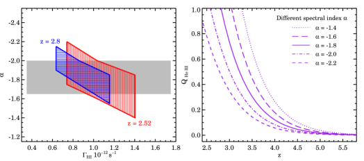
Figure 3: Left-hand panel: Joint constraints on the values of power-law index $\alpha$ of mean QSO SED (at $\lambda\leq 912$Å) and $\Gamma_{\rm HI}$ in order to satisfy the binned $\tau_{\rm\alpha}^{\rm He\,II}$ measurement as given in Table 2. These are obtained for $\epsilon^{Q}_{\rm 912}(z)$ from model A (Eq. 12). Vertical striped region shows result for lowest redshift bin with median $z=2.52$ and horizontal striped region shows results for next redshift bin with median $z=2.8$. We do not perform such analysis for highest-$z$ bin where $\tau_{\rm\alpha}^{\rm He\,II}$ is a lower limit. The gray shaded region show the range in $\alpha$ consistent with the redshift of He ii reionization $2.6<z_{\rm re}<3.0$. Right-hand panel: $Q_{\rm HeIII}(z)$ obtained for model A with different $\alpha$.

3.3 Helium reionization

We calculate reionization history of He ii by solving following differential equation to estimate the volume averaged He iii fraction ($Q_{\rm HeIII}$; Shapiro & Giroux, 1987; Madau et al., 1999; Barkana & Loeb, 2001)

$$\frac{dQ_{\rm HeIII}}{dt}=\frac{\dot{n}(t)}{\langle n_{\rm He}\rangle}-\frac{\alpha^{\rm B}_{\rm HeII}({\rm T})\,\chi\,C\langle n_{\rm He}\rangle Q_{\rm HeIII}}{a^{3}(t)}\,\,.$$ (15)

Here, $\langle n_{\rm He}\rangle=1.87\times 10^{-7}y_{p}/(4-4y_{p})$ cm^-3 is the comoving number density of helium, $\dot{n}(t)$ is comoving number density of He ii ionizing photons per unit time, C is the clumping factor of He ii, $\chi$ is number of photo-electrons per hydrogen atom, $a(t)$ is the scale factor and $\alpha^{\rm B}_{\rm HeII}({\rm T})$ is the case B recombination coefficient of He ii. Here, $\dot{n}(t)$ is obtained by

$$\dot{n}(z)=\int^{\infty}_{\nu_{228}}d\nu\,{\Big{(}\frac{\nu}{\nu_{912}}\Big{)}^{\alpha}\,\,\frac{\epsilon^{Q}_{912}(z)}{h\nu}}\,\,,$$ (16)

where, $\nu_{228}=c/228$Å Hz and $\nu_{912}=c/912$Å Hz. The solution to the Eq. (15), $Q_{\rm HeIII}$, at any redshift $z_{0}$ is given by,

$$Q_{\rm HeIII}(z_{0})=\frac{1}{\langle n_{\rm He}\rangle}\int^{\infty}_{z_{0}}dz\,\frac{\dot{n}(z)}{(1+z)H(z)}\,\times$$ (17)

$$\exp\Bigg{[}-\alpha^{\rm B}_{\rm HeII}(T)\langle n_{\rm He}\rangle\int^{z}_{z_{0}}{dz^{\prime}\frac{\chi C(z^{\prime})(1+z^{\prime})^{2}}{H(z^{\prime})}}\Bigg{]}\,\,.$$

The process of helium reionization is complete when $Q_{\rm HeIII}(z_{\rm re})$ becomes unity and that $z_{\rm re}$ is called as reionization redshift. We take clumping factor from cosmological hydrodynamical simulations of Finlator et al. (2012) as $C(z)=9.25-7.21\log(1+z)$. Note that, if instead we use $C(z)$ from Shull et al. (2012a) then the obtained $z_{\rm re}$ for model A is higher by 0.05. In the He iii regions, we take $\chi=1+[y_{p}/(2-2y_{p})]$ and T=20000K to solve for $Q_{\rm HeIII}(z)$.

4 Results and discussion

Following the procedure mentioned above, we calculate the He ii ionizing UVB and the He ii reionization history for QSO emissivities from model A and B. The results of which are discussed in the following subsections.

4.1 Model A: constraints on $\alpha$

The He ii ionizing UVB depends not only on the He ii ionizing emissivity from QSOs but also on the $\Gamma_{\rm HI}(z)$ through the calculations of $\eta$. The $\Gamma_{\rm HI}(z)$ depends on emissivity from both QSOs and galaxies. Therefore, the $f_{\rm esc}$ which decides the galaxy contribution to $\Gamma_{\rm HI}$, also affects the the He ii ionizing UVB as shown in Khaire & Srianand (2013). Here, since we directly use the measured values of $\Gamma_{\rm HI}$ to calculate the He ii ionizing UVB, we do not need to calculate the $f_{\rm esc}$ explicitly. We refer reader to Khaire et al. (2016) for the required values of $f_{\rm esc}$ to obtain the $\Gamma_{\rm HI}$ measurements that are used here.

We first consider the model A for which the emissivity is obtained from QSO luminosity function from UV and optical surveys, as given in Eq. 12. With this emissivity, we calculate the He ii ionizing UVB by varying the spectral index $\alpha$. For each $\alpha$ we also vary $\Gamma_{\rm HI}(z)$ within its 1-$\sigma$ uncertainty. The calculated UVB for each $\alpha$ and $\Gamma_{\rm HI}$ provides $\Gamma_{\rm HeII}(z)$ and $\eta(z)$. Using this $\eta(z)$ in Eq. 1 and 2, we calculate $\tau_{\rm\alpha}^{\rm He\,II}$($z$). In this way, we generate $\tau_{\rm\alpha}^{\rm He\,II}$($z$) for UVB models with different $\alpha$ and $\Gamma_{\rm HI}$. This along with $\tau_{\rm\alpha}^{\rm He\,II}$ measurements helps us to constrain values of $\alpha$.

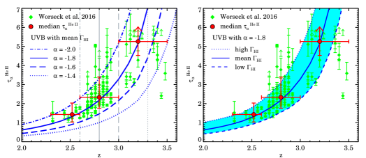
Figure 4: Left-hand panel: $\tau_{\rm\alpha}^{\rm He\,II}$(z) estimated from UVB models obtained for $\epsilon^{Q}_{\rm 912}(z)$ of model A (Eq. 12) with different spectral index $\alpha$ of the mean QSO SED (for $\lambda\leq 912$Å). Vertical gray lines with different line-styles mark the redshift of He ii reionization (see right-hand panel of Fig. 3). The UVB with $\alpha=-1.8$ reproduce the binned $\tau_{\rm\alpha}^{\rm He\,II}$ measurements. Here $\Gamma_{\rm HI}(z)$ values obtained for all the models are consistent with the mean values obtained from Becker & Bolton (2013). Right-hand panel: $\tau_{\rm\alpha}^{\rm He\,II}$(z) estimated from the UVB with $\alpha=-1.8$ with different $\Gamma_{\rm HI}$ consistent with the 1$\sigma$ higher and lower values. The shaded region show the range in $\tau_{\rm\alpha}^{\rm He\,II}$(z) due to uncertainty in the measured $\Gamma_{\rm HI}$. In both panels $\tau_{\rm\alpha}^{\rm He\,II}$ measurements by Worseck et al. (2016) are shown by diamonds and binned $\tau_{\rm\alpha}^{\rm He\,II}$ data by circles.

To obtain the binned $\tau_{\rm\alpha}^{\rm He\,II}$ measurements, as given in Table 2, we calculate the required $\alpha$ in the UVB as a function of $\Gamma_{\rm HI}(z)$ within its measured uncertainty. The results are shown in the left-hand panel of Fig. 3. Regions with vertical and horizontal stripes provide the joint constraints on $\Gamma_{\rm HI}$ and $\alpha$ that is required to obtain the binned $\tau_{\rm\alpha}^{\rm He\,II}$ at $z=2.52$ and $z=2.8$, respectively. Within 1-$\sigma$ range in measured $\Gamma_{\rm HI}(z)$, we need UVB with $-2.2<\alpha<-1.4$ at $z=2.52$ and with $-2.15<\alpha<-1.55$ at $z=2.8$. We do not calculate the required $\alpha$ to satisfy $\tau_{\rm\alpha}^{\rm He\,II}$ at highest redshift bin which is a lower limit.

The onset of large scatter in $\tau_{\rm\alpha}^{\rm He\,II}$ measurements seen at $z>2.7$ suggests that the He ii reionization has completed at $z\sim 2.7$ (Furlanetto & Dixon, 2010; Shull et al., 2010; Worseck et al., 2011; Worseck et al., 2016). At $z>z_{\rm re}$ the He ii ionizing UVB may not be uniform (see Furlanetto, 2009; Davies & Furlanetto, 2014), therefore, predicted $\tau_{\rm\alpha}^{\rm He\,II}$ may not match the measurements. To find $z_{\rm re}$, we have also calculated the reionization history. The obtained $Q_{\rm HeIII}(z)$ for models with different $\alpha$ is shown in the right-hand panel of Fig 3. The redshift of He ii reionization depends on He ii ionizing emissivity and therefore on $\alpha$. The QSO SED becomes flat for higher $\alpha$ that gives higher He ii ionizing emissivity. Therefore, higher values of $\alpha$ leads to early He ii reionization. If we impose an additional constraint on reionization redshift, such as $2.6<z_{\rm re}<3.0$ consistent with the trend in $\tau_{\rm\alpha}^{\rm He\,II}$ data, we need $-2.0<\alpha<-1.65$. The range in required $\alpha$ has shown with gray-shade in the left-hand panel of Fig 3. Combining these constraints obtained with the binned $\tau_{\rm\alpha}^{\rm He\,II}$ and the $z_{\rm re}$ together, $\alpha$ can have values from -1.6 to -2.0.

Measurements of $\alpha$ reported in the literature over last two decades are summarized in the Table 1. Let us compare the $-1.6>\alpha>-2.0$ obtained here with the recent measurements of it. Lusso et al. (2015) obtained $\alpha=-1.7\pm 0.61$ at $z\sim 2.4$ using 53 QSOs where the smallest wavelength probed by them is 600Å. Stevans et al. (2014) obtained $\alpha=-1.4\pm 0.15$ at $z<1.5$ using 159 QSOs observed from HST-COS where the smallest wavelength probed by them is 475Å. However, they had fewer than 10 QSOs which probe $\lambda<600$Å. Tilton et al. (2016) compiled 11 new QSOs from HST-COS at $1.5<z<2.1$ where the smallest wavelength probed by them is $\lambda\sim 425$Å. They combined these with 9 existing QSOs from Stevans et al. (2014) and measured $\alpha=-0.72\pm 0.26$ in wavelength range $450<\lambda<700$Å. The $-1.6>\alpha>-2.0$ obtained by us is consistent with the measurements of Lusso et al. (2015). It is within 2-$\sigma$ uncertainty from Stevans et al. (2014). However, it is 4-$\sigma$ lower than the measurements of Tilton et al. (2016). Note that, our inferred value of $\alpha$ is obtained by modeling the UVB at $\lambda\rm\leq 228$Å and at $2<z<3.5$. Here, we assumed that the QSO SED at $\lambda\leq 912$Å follows a single power-law and does not change with redshift, same as assumed in other studies. The single power-law assumption may not be true since there are no measurements that probe SED at $\lambda<400$Å. Tilton et al. (2016) suggested that a simple power-law may not be sufficient to explain the QSO SED, even at $\lambda<700$Å. Moreover, the observed QSOs spectra probing $\lambda<500$Å are biased towards most luminous QSOs. Therefore, one expects that these measurements can also be biased. Also, the mean QSO SED may have redshift dependence. It is important to study such a redshift dependence of $\alpha$ in the direct observations.

Figure 5: $\Gamma_{\rm HeII}(z)$ (left-hand panel) and $\eta_{\rm thin}(z)$ (right-hand panel) obtained from UVB models obtained for $\epsilon^{Q}_{\rm 912}(z)$ of model A (Eq. 12) with $\alpha=-1.8$. Solid, dash and dotted curves show results obtained from UVB with mean $\Gamma_{\rm HI}$, 1-$\sigma$ higher and lower $\Gamma_{\rm HI}$, respectively. Red circles show our estimates of $\Gamma_{\rm HeII}$ and $\eta_{\rm thin}$ from binned $\tau_{\rm\alpha}^{\rm He\,II}$ data, as described in Section 2.2 (Table 2).

For the UVB with different $\alpha$ and the mean value of measured $\Gamma_{\rm HI}(z)$, the obtained $\tau_{\rm\alpha}^{\rm He\,II}$($z$) is shown in the left-hand panel of Fig. 4 along with the measurements from Worseck et al. (2016) and binned $\tau_{\rm\alpha}^{\rm He\,II}$ data from Table 2. It shows that the measured $\tau_{\rm\alpha}^{\rm He\,II}$ data can be reproduced for $-1.6>\alpha>-2.0$. To reproduce binned median $\tau_{\rm\alpha}^{\rm He\,II}$ data from Table 2, the UVB with $\alpha=-1.8$ is preferred. We also mark the redshift of He ii reionization, $z_{\rm re}$ for each $\alpha$. In the post-He ii-reionization era, i.e. at $z<z_{\rm re}$, the UVB models are expected to produce the mean $\tau_{\rm\alpha}^{\rm He\,II}$ measurements and may not be at $z>z_{\rm re}$. In the right-hand panel of Fig. 4, we show $\tau_{\rm\alpha}^{\rm He\,II}$($z$) for the UVB with $\alpha=-1.8$ obtained using the mean $\Gamma_{\rm HI}(z)$ as well as 1-$\sigma$ higher and lower $\Gamma_{\rm HI}(z)$ measurements. The shaded region shows the range in $\tau_{\rm\alpha}^{\rm He\,II}$ arising from the uncertainty in $\Gamma_{\rm HI}$ measurements. Since it covers most of the $\tau_{\rm\alpha}^{\rm He\,II}$measurements at the post-He ii-reionization era, i.e at $z<2.8$, we prefer the UVB with $\alpha=-1.8$. The $\Gamma_{\rm HeII}(z)$ and $\eta_{\rm thin}(z)$ obtained from this UVB are shown in Fig. 5. Both show good agreement with the values estimated from the binned $\tau_{\rm\alpha}^{\rm He\,II}$ data (from Table 2) as explained in Section 2.2. The $\Gamma_{\rm HeII}(z)$ and $\eta_{\rm thin}(z)$ obtained for the UVB with 1-$\sigma$ higher and lower $\Gamma_{\rm HI}(z)$ show the spread in these values due to the uncertainty in $\Gamma_{\rm HI}(z)$. The very good agreement between the $\Gamma_{\rm HeII}(z)$ and $\eta_{\rm thin}(z)$ obtained from the full UVB model and the one estimated using Eq.1 to Eq. 3 (see Section 2), shows the validity of the approximations used in latter.

All the models mentioned above assume a single power-law SED of QSOs at $\lambda\leq 912$Å. The SED may not be a single-power law; rather it can consist of broken power-laws or have breaks at smaller wavelengths. To obtain the same He ii ionizing emissivity as obtained for our preferred model with $\alpha=-1.8$ but with different value of $\alpha$, a break in the mean QSO SED at a wavelength $228\leq\lambda_{b}\leq 912$Å can be applied. The value of the break, the number ($<1$) that is multiplied to the specific intensity at $\lambda\leq\lambda_{b}$, can be approximated as $(\lambda_{b}/912\rm\AA)^{(1.8+\alpha)}$. For example, when we assume $\alpha=-1.4$ consistent with measurements of Stevans et al. (2014) and Shull et al. (2012b), we verify that a break in QSO SED at $\lambda_{b}=$228Å by a factor of 0.6 gives the same $\tau_{\rm\alpha}^{\rm He\,II}$($z$) as obtained for single power-law SED with $\alpha=-1.8$. Although, the break can be applied at $228\leq\lambda_{b}\leq 912$Å, hereafter we consider the break only at $\lambda_{b}=228$Å. A slight decrease in the resultant $\Gamma_{\rm HI}$ due to such break in QSO SEDs can be compensated by marginally increasing $f_{\rm esc}$ from galaxies. This SED break can be thought as the escape fraction of He ii ionizing photons from QSOs. However, in the absence of any physical models, such a break in QSO SED and its interpretation should be treated with caution.

We have used $\alpha=-1.4$ in Khaire et al. (2016) to estimate the required $f_{\rm esc}$ of H i ionizing photons from galaxies to obtain the $\Gamma_{\rm HI}$ measurements. If we use the $\alpha=-1.6$ to $-2.0$ instead, we need an additional increase in the predicted $f_{\rm esc}$ in Khaire et al. (2016) by less than 20 %.

4.2 Model B: break in SED

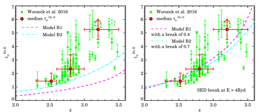
Figure 6: Left-hand panel: $\tau_{\rm\alpha}^{\rm He\,II}$($z$) obtained from the UVB with $\epsilon^{Q}_{912}(z)$ and $\alpha$ taken from model B1 (Eq. 13; dashed curve) and model B2 (Eq. 14; dot-dashed curve). Both models fail to reproduce $\tau_{\rm\alpha}^{\rm He\,II}$ measurements. Right-hand panel: $\tau_{\rm\alpha}^{\rm He\,II}$ obtained from the UVBs with the same $\epsilon^{Q}_{912}(z)$ and $\alpha$ but with appropriate SED breaks at $\lambda\leq 228$Å applied to match $\tau_{\rm\alpha}^{\rm He\,II}$ measurements. We need break of $\sim 0.4$ for model B1 (dashed curve) and $\sim 0.7$ for model B2 (dot-dashed curve). In both panels $\tau_{\rm\alpha}^{\rm He\,II}$ measurements by Worseck et al. (2016) are shown by diamonds and binned $\tau_{\rm\alpha}^{\rm He\,II}$ data by circles.

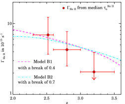
Figure 7: $\Gamma_{\rm HeII}(z)$ obtained from the UVB models with $\epsilon^{Q}_{912}(z)$ and $\alpha$ taken from model B1 (Eq. 13; dashed curve) and model B2 (Eq. 14; dot-dashed curve) with appropriate SED breaks (of 0.4 for model B1 and 0.7 for model B2) applied at ${\rm E\geq 4}$ Ryd to match the $\tau_{\rm\alpha}^{\rm He\,II}$ measurements as shown in the right-hand panel of Fig. 6. The red circles show our estimates of $\Gamma_{\rm HeII}$ from binned $\tau_{\rm\alpha}^{\rm He\,II}$ data, as described in Section 2.2 (Table 2).

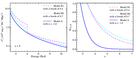
Figure 8: The $\epsilon^{Q}_{\nu}$ at different energies for $z=3$ (left-hand panel) and $Q_{\rm HeIII}(z)$ (right-hand panel) obtained from different models. These models are model B1 (Eq. 13 and $\alpha=-1.4$; dashed curve) with SED break of 0.4 at ${\rm E}\geq 4$Ryd, model B2 (Eq. 14 and $\alpha=-1.7$; dot-dashed curve) with SED break of 0.7 at ${\rm E}\geq 4$Ryd and model A (Eq. 12 and $\alpha=-1.8$; solid curve) with no break in SED.

Now we consider the two combinations of $\alpha$ and $\epsilon^{Q}_{912}(z)$ from model B (Eq. 13 and 14) that include the emissivity from low-luminosity X-ray selected QSOs of Giallongo et al. (2015) at $z>4$ and reionize H i alone. The model B1 (Eq. 13) uses $\alpha=-1.4$ and the model B2 (Eq. 14) uses $\alpha=-1.7$. We calculate the UVB and $\tau_{\rm\alpha}^{\rm He\,II}$ for these models. The results are shown in the left-hand panel of Fig. 6. The comparison with the data shows that these models can not reproduce the $\tau_{\rm\alpha}^{\rm He\,II}$ measurements.

These models also predict higher redshift for completion of He ii reionization, as $z_{\rm re}=5.2$ for model B1 and $z_{\rm re}=4.5$ for model B2. It is one of the issues of such high QSO emissivity models. Therefore, these models need modifications. We can not change values of $\alpha$ since they are already adjusted along with $\epsilon^{Q}_{912}(z)$ to reionize H i alone without requiring any contribution from galaxies and to satisfy different observational constraints on H i reionization. However, we can break the respective SEDs at $\lambda\leq 228$Å so that the H i ionizing emissivity and its prediction for H i reionization remains the same but the He ii ionizing emissivity reduces.

We estimate the $\tau_{\rm\alpha}^{\rm He\,II}$ for the UVB obtained with different SED breaks at $\lambda\leq 228$Å. We find that for model B1, we need SED break of a factor $\sim$0.4 at $\lambda\leq 228$Å to reproduce the $\tau_{\rm\alpha}^{\rm He\,II}$ measurements. For model B2, since it already has steeper SED with $\alpha=-1.7$, a SED break of factor $\sim$0.7 at $\lambda\leq 228$Å is needed. The $\tau_{\rm\alpha}^{\rm He\,II}$ obtained in these models with such modifications are shown in the right-hand panel of the Fig. 6. The values of $\Gamma_{\rm HeII}$ obtained for these models are shown in Fig. 7. These are in good agreement with the values estimate using binned $\tau_{\rm\alpha}^{\rm He\,II}$ data. In the left-hand panel of Fig. 8 we show the $\epsilon^{Q}_{\nu}$ at $z=3$ for an illustrative purpose from the model B1 and B2 with the SED breaks obtained here. For comparison, we also show the $\epsilon^{Q}_{\nu}$ at $z=3$ from model A with no SED break. In all three models, although the H i ionizing emissivities are different, the respective breaks in model B1 and B2 achieve the similar He ii ionizing emissivities as model A. With such modifications, these models also predict lower He ii reionization redshift. For model B1, the $z_{\rm re}$ is now 3.4 and for model B2 it is $3.3$. The $Q_{\rm HeIII}(z)$ is shown in the right-hand panel of Fig. 8. Note that if we use the clumping factor for He ii from Shull et al. (2012a) then the obtained $z_{\rm re}$ is higher by additional 0.2. The $\epsilon^{Q}_{912}(z)$ values taken in these models are not significantly different from model A at $2.3<z<3.2$ (see Fig. 2). Therefore, the models with SED steeper than $\alpha=-1.7$ can be consistent with the $\tau_{\rm\alpha}^{\rm He\,II}$ measurements at $z<3$ but can not reproduce the trend in increasing $\tau_{\rm\alpha}^{\rm He\,II}$ at $z>3$. Also, in such models $\epsilon^{Q}_{912}(z)$ should be higher than the model B2 to reionize H i alone that will require higher emissivity than Giallongo et al. (2015) and it may not be consistent with upper limits on the unresolved X-ray background at high-z (see Haardt & Salvaterra, 2015).

The main difference between the model A and model B (both B1 and B2) is the He ii reionization history. Even though the model B1 and B2 are modified with the SED breaks to reproduce the $\tau_{\rm\alpha}^{\rm He\,II}$ measurements, the $Q_{\rm HeIII}(z)$ predicted by them differ significantly from model A, as shown in the right-hand panel of Fig. 8. For example, at $z\sim 4$ (5) in model A only 10 (3) per cent of the volume in the Universe is in He iii as compared to the 60 (40) per cent in the model B. The He ii reionization process is more extended and slower in model B as compared to model A. This difference will show imprints on the thermal history of the IGM (see also Mitra et al., 2016; D’Aloisio et al., 2016) which will be crucial to distinguish these models.

To distinguish model A where galaxies dominate the H i reionization and model B where QSOs alone reionize H i, apart from the thermal history of the IGM the detection of the 21 cm brightness temperature fluctuations will be crucial (Kulkarni et al., 2017). Also, the independent observational confirmations of the QSO luminosity function presented by Giallongo et al. (2015) is needed for considering such high QSO emissivity models. Note that, similar studies such as Weigel et al. (2015), Georgakakis et al. (2015), Ricci et al. (2017) and Akiyama et al. (2017) do not confirm the results of Giallongo et al. (2015).

4.3 Model uncertainties

Here, we discuss the uncertainties in our models and how they affect the results presented in the preceding subsections. The estimates of $\tau_{\rm\alpha}^{\rm He\,II}$ depend on three quantities, the assumed $b$-parameter, the $N^{\rm min}_{\rm HI}$ and the $\eta$ obtained from the UVB.

We took $b=28$ km s^-1 for H i as well as He ii assuming that the turbulence dominates the Doppler broadening. If the thermal broadening dominates the $b$-parameter then the $b$ for He ii becomes 14 km s^-1. This $b$-parameter gives 38% smaller $\tau_{\rm\alpha}^{\rm He\,II}$ as compared to the one obtained earlier for each UVB model presented here. To match the $\tau_{\rm\alpha}^{\rm He\,II}$ measurements this model will require more steep QSO SED (i.e small $\alpha$) or small value of break in the QSO SED at $\lambda\leq 228$Å. With this $b$, we find that for QSO emissivity from model A, we need $-1.8>\alpha>-2.0$ to reproduce the $\tau_{\rm\alpha}^{\rm He\,II}$ measurements and to obtain $z_{\rm re}\leq 3$. For model B1 and B2, we need a break in QSO SED of factor 0.3 and 0.5 at $\lambda\leq 228$Å, respectively, to match the $\tau_{\rm\alpha}^{\rm He\,II}$ measurements.

The value of $N^{\rm min}_{\rm HI}$ is crucial for $\tau_{\rm\alpha}^{\rm He\,II}$ since the fit to the $f(N_{\rm HI},z)$ is very steep at low values of $N_{\rm HI}$. We took $N^{\rm min}_{\rm HI}$ to have minimum equivalent width of $5.2\times 10^{-3}{\rm\AA}$, which reproduce the $\tau_{\rm\alpha}^{\rm H\,I}$ measurements with $N^{\rm min}_{\rm HI}=10^{12}$ cm^-2. The $\tau_{\rm\alpha}^{\rm He\,II}$ does not converge rapidly if we extrapolate the fitting form of the observed $f(N_{\rm HI},z)$ to smaller $N_{\rm HI}$ values. However, note that the Inoue et al. (2014) obtained the fit to $f(N_{\rm HI},z)$ at low $N_{\rm HI}$ values using the measurements from Kim et al. (2013) that probe minimum $N_{\rm HI}\sim 10^{12.7}$ cm^-2. For $N_{\rm HI}<10^{12.5}$ cm^-2 the $f(N_{\rm HI},z)$ is rather flat and even shows decreasing trend (refer to Figure 7 from D’Odorico et al., 2016). If we assume that $f(N_{\rm HI},z)$ is constant or decreasing at $N_{\rm HI}<10^{12}$ or $10^{12.5}$ cm^-2 the $\tau_{\rm\alpha}^{\rm He\,II}$ converges rapidly. When we use a constant $f(N_{\rm HI},z)$ at $N_{\rm HI}<10^{12}$ cm^-2 and $N^{\rm min}_{\rm HI}=0$, we find that the maximum increase in $\tau_{\rm\alpha}^{\rm He\,II}$ at $z<3.5$ is less than 10% as compared to the value we obtain by assuming $N^{\rm min}_{\rm HI}=(16/\eta_{\rm thin})\times 10^{12}\,{\rm cm^{-2}}$ and less than 20% by assuming $N^{\rm min}_{\rm HI}=10^{12}\,{\rm cm^{-2}}$. This does not affect our results significantly.

For the measured values of $\Gamma_{\rm HI}$, values of $\eta$ depend on He ii ionizing emissivity. We discussed the constraints on the SED, however, we assumed fixed $\epsilon^{Q}_{912}(z)$ values in each model. As mentioned earlier, we can not change $\epsilon^{Q}_{912}(z)$ without changing $\alpha$ in the models that alone reionize H i, such as the model B1 and B2. However, we can change it in the model A. If we uniformly reduce the $\epsilon^{Q}_{912}(z)$ in our model A by 10% (20%) at $z>2$ allowed by the uncertainties in the QSO luminosity functions, we find that the $\eta$ increases due to a decrease in He ii ionizing emissivity. This leads to higher $\tau_{\rm\alpha}^{\rm He\,II}$ by $10-15$% ($25-40$%) over redshift $2-3.5$. For such models, we find that $-1.5>\alpha>-1.9$ is needed to reproduce the $\tau_{\rm\alpha}^{\rm He\,II}$ measurements.

Note that the variation in $\tau_{\rm\alpha}^{\rm He\,II}$ arising from all these uncertainties is smaller than the one arising from the uncertainty in the measured $\Gamma_{\rm HI}$ itself (see the right-hand panel of Fig. 4). In future, more stringent constraints on the QSO SED can be obtained using accurate measurements of $\Gamma_{\rm HI}$ and more observations of $\tau_{\rm\alpha}^{\rm He\,II}$ in the post-He ii-reionization era ($z<2.6$). Currently, there are only two sightlines, HE2347$-$4342 and HS1700$+$6416, that probe He ii Lyman-$\alpha$ forest at $z<2.6$.

5 Summary

Here, we present a method that constrains the He ii ionizing emissivity using $\tau_{\rm\alpha}^{\rm He\,II}$ measurement obtained from He ii Lyman-$\alpha$ forest and the distribution of H i in the IGM obtained from H i Lyman-$\alpha$ forest. The method uses our cosmological radiative transfer code developed to calculate the UVB by varying the input He ii ionizing emissivity to be consistent with $\tau_{\rm\alpha}^{\rm He\,II}$ measurements. The He ii ionizing emissivity depends on the QSO emissivity obtained from their luminosity functions and the mean QSO SED extrapolated at $\rm E\geq 4$ Ryd. The latter has been observationally constrained only up to $\rm E\sim 2.3$ Ryd. We constrain the QSO SED at $\rm E\geq 4$ Ryd required to satisfy the recent measurements of $\tau_{\rm\alpha}^{\rm He\,II}$ (Worseck et al., 2016) using models of updated QSO emissivity at 1 Ryd (Khaire & Srianand, 2015a) and H i distribution of the IGM (Inoue et al., 2014) in our UVB code. We have also calculated the $\Gamma_{\rm HeII}$ (provided in Table 2) from the binned $\tau_{\rm\alpha}^{\rm He\,II}$ data which depends only on the H i column density distribution at $N_{\rm HI}<10^{16}$ cm^-2 and the $\Gamma_{\rm HI}$ measurements at $z>2.2$ (Becker & Bolton, 2013).

The mean SED obtained from QSO composite spectra is usually approximated as a power-law $f_{\rm E}\propto\rm E^{\alpha}$ at $\rm E\geq 1$ Ryd. For QSO emissivity obtained using their luminosity functions from optical surveys, we find that the $\tau_{\rm\alpha}^{\rm He\,II}$ measurements are well reproduced when we use the power-law index $-1.6<\alpha<-2.0$. The UVB models with this $\alpha$ not only reproduce the majority of the $\tau_{\rm\alpha}^{\rm He\,II}$ measurements but also reionize He ii at $2.6<z_{\rm re}<3.0$, consistent with the trend seen in the $\tau_{\rm\alpha}^{\rm He\,II}$ data. The $-1.6<\alpha<-2.0$ constrained here is consistent with the measurements of Lusso et al. (2015) and Stevans et al. (2014) but 4-$\sigma$ lower than the measurement by Tilton et al. (2016). We prefer the UVB model with $\alpha=-1.8$ because it reproduces the $\tau_{\rm\alpha}^{\rm He\,II}$ measurements and our estimated $\Gamma_{\rm HeII}$ values within the uncertainties in the measured $\Gamma_{\rm HI}$.

We also consider models of QSO emissivity that include the luminosity function obtained from low-luminosity X-ray selected QSOs presented by Giallongo et al. (2015) at $z>4$. These models are constructed such that they can reionize H i without requiring any contribution from galaxies (MH15 Khaire et al., 2016) when extrapolated to $z>6$. We find that these models can not reproduce $\tau_{\rm\alpha}^{\rm He\,II}$ measurements and need modifications to reduce the He ii ionizing emissivity. For such a model with $\alpha=-1.4$ from Khaire et al. (2016), we need a break in mean QSO SED at $\rm E\geq 4$ Ryd of a factor $\sim 0.4$. Similarly, for a model with $\alpha=-1.7$ from MH15 we need break of a factor $\sim 0.7$ (see the left-hand panel of Fig. 8 for illustration of such SED breaks). These modified models give epoch of He ii reionization at $3.3-3.4$ which is significantly smaller than $4.5-5.2$ obtained without such modifications. However, even with such modifications the He ii reionization history is significantly different from standard models (see the right-hand panel of Fig. 8) which do not include the luminosity function of Giallongo et al. (2015). The thermal history of the IGM will play crucial role in distinguishing these models.

The method presented here requires better observational constraints on both $\Gamma_{\rm HI}$ and the H i distribution in the IGM, as well as measurements of $\tau_{\rm\alpha}^{\rm He\,II}$ over a large redshift range, to accurately constrain the mean QSO SED together with its redshift dependence. Using different QSO SEDs provides significantly different UVB at He ii ionizing wavelengths. Observations of metal line ratios tracing lower and higher energies around He ii ionization potential (such as C iv and Si iv) can be considered to test different models of the UVB (see for e.g., Fechner, 2011). We plan to carry such studies in future.

References

- Akiyama et al. (2017) Akiyama M., et al., 2017, preprint, (arXiv:1704.05996)
- Barkana & Loeb (2001) Barkana R., Loeb A., 2001, Phys. Rep., 349, 125
- Becker & Bolton (2013) Becker G. D., Bolton J. S., 2013, MNRAS, 436, 1023
- Becker et al. (2011) Becker G. D., Bolton J. S., Haehnelt M. G., Sargent W. L. W., 2011, MNRAS, 410, 1096
- Becker et al. (2013) Becker G. D., Hewett P. C., Worseck G., Prochaska J. X., 2013, MNRAS, 430, 2067
- Bergeron et al. (2002) Bergeron J., Aracil B., Petitjean P., Pichon C., 2002, A&A, 396, L11
- Bolton & Haehnelt (2007) Bolton J. S., Haehnelt M. G., 2007, MNRAS, 382, 325
- Bolton et al. (2010) Bolton J. S., Becker G. D., Wyithe J. S. B., Haehnelt M. G., Sargent W. L. W., 2010, MNRAS, 406, 612
- Bolton et al. (2012) Bolton J. S., Becker G. D., Raskutti S., Wyithe J. S. B., Haehnelt M. G., Sargent W. L. W., 2012, MNRAS, 419, 2880
- Calverley et al. (2011) Calverley A. P., Becker G. D., Haehnelt M. G., Bolton J. S., 2011, MNRAS, 412, 2543
- Carswell et al. (2002) Carswell B., Schaye J., Kim T.-S., 2002, ApJ, 578, 43
- Compostella et al. (2013) Compostella M., Cantalupo S., Porciani C., 2013, MNRAS, 435, 3169
- Croom et al. (2009) Croom S. M., et al., 2009, MNRAS, 399, 1755
- D’Aloisio et al. (2016) D’Aloisio A., McQuinn M., Davies F. B., Furlanetto S. R., 2016, preprint, (arXiv:1611.02711)
- D’Odorico et al. (2016) D’Odorico V., et al., 2016, MNRAS, 463, 2690
- Danforth & Shull (2005) Danforth C. W., Shull J. M., 2005, ApJ, 624, 555
- Davies & Furlanetto (2014) Davies F. B., Furlanetto S. R., 2014, MNRAS, 437, 1141
- Fan et al. (2006) Fan X., et al., 2006, AJ, 132, 117
- Fardal et al. (1998) Fardal M. A., Giroux M. L., Shull J. M., 1998, AJ, 115, 2206
- Faucher-Giguère et al. (2008) Faucher-Giguère C.-A., Prochaska J. X., Lidz A., Hernquist L., Zaldarriaga M., 2008, ApJ, 681, 831
- Faucher-Giguère et al. (2009) Faucher-Giguère C.-A., Lidz A., Zaldarriaga M., Hernquist L., 2009, ApJ, 703, 1416
- Fechner (2011) Fechner C., 2011, A&A, 532, A62
- Fechner et al. (2006) Fechner C., et al., 2006, A&A, 455, 91
- Ferland et al. (2013) Ferland G. J., et al., 2013, Rev. Mex. Astron. Astrofis., 49, 137
- Finlator et al. (2012) Finlator K., Oh S. P., Özel F., Davé R., 2012, MNRAS, 427, 2464
- Furlanetto (2009) Furlanetto S. R., 2009, ApJ, 703, 702
- Furlanetto & Dixon (2010) Furlanetto S. R., Dixon K. L., 2010, ApJ, 714, 355
- Georgakakis et al. (2015) Georgakakis A., et al., 2015, MNRAS, 453, 1946
- Giallongo et al. (2015) Giallongo E., et al., 2015, A&A, 578, A83
- Glikman et al. (2011) Glikman E., Djorgovski S. G., Stern D., Dey A., Jannuzi B. T., Lee K.-S., 2011, ApJ, 728, L26
- Gunn & Peterson (1965) Gunn J. E., Peterson B. A., 1965, ApJ, 142, 1633
- Haardt & Madau (1996) Haardt F., Madau P., 1996, ApJ, 461, 20
- Haardt & Madau (2012) Haardt F., Madau P., 2012, ApJ, 746, 125
- Haardt & Salvaterra (2015) Haardt F., Salvaterra R., 2015, A&A, 575, L16
- Hussain et al. (2015) Hussain T., Muzahid S., Narayanan A., Srianand R., Wakker B. P., Charlton J. C., Pathak A., 2015, MNRAS, 446, 2444
- Hussain et al. (2017) Hussain T., Khaire V., Srianand R., Muzahid S., Pathak A., 2017, MNRAS, 466, 3133
- Inoue et al. (2006) Inoue A. K., Iwata I., Deharveng J.-M., 2006, MNRAS, 371, L1
- Inoue et al. (2014) Inoue A. K., Shimizu I., Iwata I., Tanaka M., 2014, MNRAS, 442, 1805
- Kashikawa et al. (2015) Kashikawa N., et al., 2015, ApJ, 798, 28
- Khaire & Srianand (2013) Khaire V., Srianand R., 2013, MNRAS, 431, L53
- Khaire & Srianand (2015a) Khaire V., Srianand R., 2015a, MNRAS, 451, L30
- Khaire & Srianand (2015b) Khaire V., Srianand R., 2015b, ApJ, 805, 33
- Khaire et al. (2016) Khaire V., Srianand R., Choudhury T. R., Gaikwad P., 2016, MNRAS, 457, 4051
- Khrykin et al. (2017) Khrykin I. S., Hennawi J. F., McQuinn M., 2017, ApJ, 838, 96
- Kim et al. (2013) Kim T.-S., Partl A. M., Carswell R. F., Müller V., 2013, A&A, 552, A77
- Kirkman et al. (2007) Kirkman D., Tytler D., Lubin D., Charlton J., 2007, MNRAS, 376, 1227
- Kriss et al. (2001) Kriss G. A., et al., 2001, Science, 293, 1112
- Kulkarni et al. (2017) Kulkarni G., Choudhury T. R., Puchwein E., Haehnelt M. G., 2017, preprint, (arXiv:1701.04408)
- La Plante & Trac (2016) La Plante P., Trac H., 2016, ApJ, 828, 90
- Lidz et al. (2010) Lidz A., Faucher-Giguère C.-A., Dall’Aglio A., McQuinn M., Fechner C., Zaldarriaga M., Hernquist L., Dutta S., 2010, ApJ, 718, 199
- Lusso et al. (2015) Lusso E., Worseck G., Hennawi J. F., Prochaska J. X., Vignali C., Stern J., O’Meara J. M., 2015, MNRAS, 449, 4204
- Madau & Haardt (2015) Madau P., Haardt F., 2015, ApJ, 813, L8
- Madau & Meiksin (1994) Madau P., Meiksin A., 1994, ApJ, 433, L53
- Madau et al. (1999) Madau P., Haardt F., Rees M. J., 1999, ApJ, 514, 648
- Masters et al. (2012) Masters D., et al., 2012, ApJ, 755, 169
- McGreer et al. (2013) McGreer I. D., et al., 2013, ApJ, 768, 105
- McGreer et al. (2015) McGreer I. D., Mesinger A., D’Odorico V., 2015, MNRAS, 447, 499
- McQuinn & Worseck (2014) McQuinn M., Worseck G., 2014, MNRAS, 440, 2406
- McQuinn et al. (2009) McQuinn M., Lidz A., Zaldarriaga M., Hernquist L., Hopkins P. F., Dutta S., Faucher-Giguère C.-A., 2009, ApJ, 694, 842
- Meiring et al. (2013) Meiring J. D., Tripp T. M., Werk J. K., Howk J. C., Jenkins E. B., Prochaska J. X., Lehner N., Sembach K. R., 2013, ApJ, 767, 49
- Miralda-Escude & Ostriker (1990) Miralda-Escude J., Ostriker J. P., 1990, ApJ, 350, 1
- Mitra et al. (2016) Mitra S., Choudhury T. R., Ferrara A., 2016, preprint, (arXiv:1606.02719)
- Moretti et al. (2012) Moretti A., Vattakunnel S., Tozzi P., Salvaterra R., Severgnini P., Fugazza D., Haardt F., Gilli R., 2012, A&A, 548, A87
- Muzahid et al. (2011) Muzahid S., Srianand R., Petitjean P., 2011, MNRAS, 410, 2193
- Muzahid et al. (2012) Muzahid S., Srianand R., Bergeron J., Petitjean P., 2012, MNRAS, 421, 446
- Narayanan et al. (2012) Narayanan A., Savage B. D., Wakker B. P., 2012, ApJ, 752, 65
- Pachat et al. (2016) Pachat S., Narayanan A., Muzahid S., Khaire V., Srianand R., Wakker B. P., Savage B. D., 2016, MNRAS, 458, 733
- Padmanabhan (2002) Padmanabhan T., 2002, Theoretical Astrophysics - Volume 3, Galaxies and Cosmology, doi:10.2277/0521562422.
- Palanque-Delabrouille et al. (2013) Palanque-Delabrouille N., et al., 2013, A&A, 551, A29
- Paresce et al. (1980) Paresce F., McKee C. F., Bowyer S., 1980, ApJ, 240, 387
- Peebles (1993) Peebles P. J. E., 1993, Principles of Physical Cosmology
- Peeples et al. (2014) Peeples M. S., Werk J. K., Tumlinson J., Oppenheimer B. D., Prochaska J. X., Katz N., Weinberg D. H., 2014, ApJ, 786, 54
- Planck Collaboration et al. (2016) Planck Collaboration et al., 2016, A&A, 594, A13
- Ricci et al. (2017) Ricci F., Marchesi S., Shankar F., La Franca F., Civano F., 2017, MNRAS, 465, 1915
- Ross et al. (2013) Ross N. P., et al., 2013, ApJ, 773, 14
- Savage et al. (2005) Savage B. D., Lehner N., Wakker B. P., Sembach K. R., Tripp T. M., 2005, ApJ, 626, 776
- Savage et al. (2011) Savage B. D., Narayanan A., Lehner N., Wakker B. P., 2011, ApJ, 731, 14
- Schaye (2001) Schaye J., 2001, ApJ, 559, 507
- Schenker et al. (2014) Schenker M. A., Ellis R. S., Konidaris N. P., Stark D. P., 2014, ApJ, 795, 20
- Schulze et al. (2009) Schulze A., Wisotzki L., Husemann B., 2009, A&A, 507, 781
- Scott et al. (2004) Scott J. E., Kriss G. A., Brotherton M., Green R. F., Hutchings J., Shull J. M., Zheng W., 2004, ApJ, 615, 135
- Shapiro & Giroux (1987) Shapiro P. R., Giroux M. L., 1987, ApJ, 321, L107
- Shapiro et al. (1994) Shapiro P. R., Giroux M. L., Babul A., 1994, ApJ, 427, 25
- Shull et al. (1999) Shull J. M., Roberts D., Giroux M. L., Penton S. V., Fardal M. A., 1999, AJ, 118, 1450
- Shull et al. (2004) Shull J. M., Tumlinson J., Giroux M. L., Kriss G. A., Reimers D., 2004, ApJ, 600, 570
- Shull et al. (2010) Shull J. M., France K., Danforth C. W., Smith B., Tumlinson J., 2010, ApJ, 722, 1312
- Shull et al. (2012a) Shull J. M., Harness A., Trenti M., Smith B. D., 2012a, ApJ, 747, 100
- Shull et al. (2012b) Shull J. M., Stevans M., Danforth C. W., 2012b, ApJ, 752, 162
- Shull et al. (2014) Shull J. M., Danforth C. W., Tilton E. M., 2014, ApJ, 796, 49
- Simcoe et al. (2004) Simcoe R. A., Sargent W. L. W., Rauch M., 2004, ApJ, 606, 92
- Songaila (2001) Songaila A., 2001, ApJ, 561, L153
- Songaila & Cowie (1996) Songaila A., Cowie L. L., 1996, AJ, 112, 335
- Stevans et al. (2014) Stevans M. L., Shull J. M., Danforth C. W., Tilton E. M., 2014, ApJ, 794, 75
- Syphers & Shull (2013) Syphers D., Shull J. M., 2013, ApJ, 765, 119
- Syphers et al. (2011) Syphers D., Anderson S. F., Zheng W., Meiksin A., Haggard D., Schneider D. P., York D. G., 2011, ApJ, 726, 111
- Telfer et al. (2002) Telfer R. C., Zheng W., Kriss G. A., Davidsen A. F., 2002, ApJ, 565, 773
- Tilton et al. (2016) Tilton E. M., Stevans M. L., Shull J. M., Danforth C. W., 2016, ApJ, 817, 56
- Tripp et al. (2008) Tripp T. M., Sembach K. R., Bowen D. V., Savage B. D., Jenkins E. B., Lehner N., Richter P., 2008, ApJS, 177, 39
- Weigel et al. (2015) Weigel A. K., Schawinski K., Treister E., Urry C. M., Koss M., Trakhtenbrot B., 2015, MNRAS, 448, 3167
- Worseck et al. (2011) Worseck G., et al., 2011, ApJ, 733, L24
- Worseck et al. (2016) Worseck G., Prochaska J. X., Hennawi J. F., McQuinn M., 2016, ApJ, 825, 144
- Wyithe & Bolton (2011) Wyithe J. S. B., Bolton J. S., 2011, MNRAS, 412, 1926
- Zheng et al. (1997) Zheng W., Kriss G. A., Telfer R. C., Grimes J. P., Davidsen A. F., 1997, ApJ, 475, 469
- Zheng et al. (2004) Zheng W., et al., 2004, ApJ, 605, 631