Cooperative epidemic spreading on a two-layered interconnected network

Abstract

This study is concerned with the dynamical behaviors of epidemic spreading over a two-layered interconnected network. Three models in different levels are proposed to describe cooperative spreading processes over the interconnected network, wherein the disease in one network can spread to the other. Theoretical analysis is provided for each model to reveal that the global epidemic threshold in the interconnected network is not larger than the epidemic thresholds for the two isolated layered networks. In particular, in an interconnected homogenous network, detailed theoretical analysis is presented, which allows quick and accurate calculations of the global epidemic threshold. Moreover, in an interconnected heterogeneous network with inter-layer correlation between node degrees, it is found that the inter-layer correlation coefficient has little impact on the epidemic threshold, but has significant impact on the total prevalence. Simulations further verify the analytical results, showing that cooperative epidemic processes promote the spreading of diseases.

I Introduction

Epidemic spreading, as an important dynamic process taking place on complex networks, has stimulated wide interest in the past two decades. Many spreading processes have been studied on isolated networks Pastor-Satorras and Vespignani (2001); Newman (2002); Motter et al. (2002); Eames and Keeling (2004); Liljeros et al. (2003); Reed (2006). However, in the real-world, an epidemic process may spread across different networks. For example, Avian influenza, such as 2009 H1N1 and 2013 H7N9, can spread from poultry to humans. A natural extension of the study is to use an interacting network model to analyze real-world epidemic processes, where a disease is able to spread from one network to another. Recent studies have shown that comprising interconnected networks can more accurately simulate real-world situations Saumell-Mendiola et al. (2012); Dickison et al. (2012); Yagan et al. (2013); Domenico et al. (2013); Zhao et al. (2014a); Xu et al. (2015); Li et al. (2015). The classical SIS and SIR models were studied on interconnected networks. In Saumell-Mendiola et al. (2012), a heterogeneous mean-field approach was developed to calculate conditions for the emergence of an endemic state, which revealed that the global epidemic threshold of interconnected networks is smaller than the threshold of each individual network. In Dickison et al. (2012), the SIR model was studied on interconnected networks, which showed that for strongly interconnected networks, the endemic state occurs or dies out simultaneously in each component network. Using generating function and bond percolation theory, multiple routes transmitted epidemic process was modeled following the SIR model in multiplex networks Zhao et al. (2014a), which revealed that an endemic state can emerge in multiplex networks even if the layers are well below their respective epidemic thresholds. In Cozzo et al. (2013), perturbation theory was used to analyze epidemic thresholds of networks, which revealed that the spectral radius of the whole network matrix is never smaller than that of each submatrix. Thus, the epidemic threshold of the whole network is always not larger than the thresholds of the isolated networks. It was found that the epidemic threshold of a multiplex network is governed by the layer that contains the largest eigenvalue of the contact matrixCozzo et al. (2013); Wang et al. (2013). In Sanz et al. (2014), a framework was proposed to describe the spreading dynamics of two diseases, it was found there are regions of the parameter space, in which a disease s outbreak is conditioned to the prevalence of the other disease.

The interplay between awareness and disease spread processes is a key issue in studying epidemics. With the interaction of two processes, such as the spreading of a disease and the spreading of the information awareness to prevent infection, epidemic spreading promotes wider information awareness which can further protract infection. A conclusion is that information awareness can suppress epidemic spreading Clara et al. (2013); Granell et al. (2014). Therefore, epidemic spreading processes on multiplex networks exhibit rich phase diagrams of intertwined effects. While the study of uncorrelated complex networks is a fundamental step for investigating many complex systems, in a realistic interconnected network, inter-layer degree correlation is expected to exist. For example, in a social network, a person with a large number of links in one network layer is likely to have many links in other types of network layers that reflect different kinds of social relations, such as being a friendly personLee et al. (2012).

Recent works have shown that correlated multiplexity is ubiquitous in the world trade system Barigozzi et al. (2009), as well as in transportation network systemsParshani et al. (2011); Xu et al. (2011). Due to their impact on network robustness Parshani et al. (2011); Buldyrev et al. (2011) and percolation properties Nicosia and Latora (2015); Lee et al. (2012), multiplex networks has been extensively studied. In Wang et al. (2014), the impact of inter-layer correlations on epidemic processes was studied regarding awareness in disease networks. With a degree correlation between double-layer random awareness networks and disease spreading, there is a strong evidence that an epidemic can be suppressed through large-degree nodes Wang et al. (2014), thus it is possible to effectively mitigate an epidemic disease by information diffusion via hub nodes with high degree centrality.

The structure of a complex network can be characterized by its degree property, which represents the type of interaction between components (nodes). In terms of degree distribution, complex networks can be classified into homogeneous and heterogeneous networksPastor-Satorras and Vespignani (2001); Tanaka (2012). Homogeneous networks, such as random graphs and small-world models, possess the Poisson type of degree distributions, with most nodes basically bearing the mean degree. Heterogeneous networks, such as scale-free networks, exhibit a power-law degree distribution. This kind of distribution implies that a small portion of nodes have very large degrees compared to the average degree of the network. However, degree distribution gives information about the connectivity probability at the level of a group of nodes but not individual nodes. Thus, to obtain more detailed description for individual nodes, it is necessary to propose a model describing spreading dynamics at the individual level.

The aforementioned works focus on multiplex networks, in which the nodes in each layer are the same, and each node in one layer is only connected to its counterparts in the other layer. However, many complex systems contain layers with different kinds of nodes, such as homosexual and heterosexual networks of sexual contacts, transportation networks which depend on different layers such as air routes, railways and roads. Furthermore, in these complex systems, a node in one layer can connect with various nodes in the other layer. Thus, the study of epidemic spreading on interconnected networks, in which different layers have different numbers or types of nodes, is of more practical significance.

The present study focuses on how the structures of complex networks and the inter-layer connections determine the epidemic thresholds of a two-layered (extendable to more) interconnected network. Three dynamical models are proposed to describe cooperative spreading processes on an interconnected homogenous or heterogeneous network. The first one is the spreading dynamics on the whole network of two homogeneous layered networks. The second is the spreading dynamics in groups of nodes with identical degrees on a two-layered heterogeneous network with inter-layer correlations. The last one is the spreading dynamical model at the individual level on a two-layered heterogeneous network without inter-layer correlations. This last model assumes that probabilities of nodes being infected are independent random variables. Theoretical analysis and numerical simulations are used to investigate the cooperative spreading processes.

The rest of the paper is organized as follows. Three models and theoretical analysis are presented in Sec. II. Numerical simulations are presented to illustrate the behaviors of cooperative spreading processes in Sec. III. Finally, conclusions are given in Sec. IV with some discussions.

II Network modeling and preliminaries

Consider a two-layered interconnected network, network layer $A$ of size $N$ and $B$ of size $M$, which have different connectivities. Use network $AB$ $(BA)$, both of size $M+N$, to denote inter-layer connectivity from layer $A$ ($B$) to $B$ ($A$). The inter-layer connectivity randomly correlates between the two layers. An example of two interconnected networks is shown in Fig.1.

The classical susceptible-infected-susceptible (SIS) model Pastor-Satorras and Vespignani (2001) is used to describe the spreading dynamics on the interconnected network. In the network, each node is either in the susceptible (S) or infected (I) state, and the links represent the connections between nodes along which the infection can propagate. At each time step, susceptible (S) nodes may be infected by infected nodes within the same layer with a certain probability or in other layers with a certain probability simultaneously. On the other hand, infected nodes are recovered spontaneously with a certain probability on each layer. Let $\lambda_{a}$ $(\lambda_{b})$ be the internal infection rate in layer $A~{}(B)$, and $\lambda_{ba}$ ($\lambda_{ab}$) be the inter-layer infection rate from nodes in $B$ ($A$) to nodes in $A$ ($B$). Infected nodes are recovered with rate $\mu_{a}$ ($\mu_{b}$) in $A~{}(B)$.

II.1 A two-layered randomly-correlated homogeneous network

Let network layers $A$ and $B$ be two homogeneous networks that are connected without relying on degree correlations. Nodes in layer $A$ $(B)$ are characterized by average degree $\langle k_{a}\rangle$ ($\langle k_{b}\rangle$), and $\langle k_{ba}\rangle$ represents the average inter-layer connections of nodes in $A$ and $\langle k_{ab}\rangle$ in $B$. The fractions of infected nodes in $A$ and $B$ are denoted by $\rho^{A}(t)$ and $\rho^{B}(t)$, respectively. Thus, the evolution processes can be written as

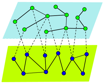
Figure 1: The interconnected two-layer network is different from layer to layer, and inter-layer connectivity randomly correlates between the two layers. Solid and dashed lines represent internal and inter-layer connections, respectively.

$$\frac{d\rho^{A}(t)}{dt} =-\mu_{a}\rho^{A}(t)+\lambda_{a}\langle k_{a}\rangle\rho^{A}(t)(1-\rho^{A}(t))$$

$$+\lambda_{ba}\langle k_{ba}\rangle\rho^{B}(t)(1-\rho^{A}(t)),$$

$$\frac{d\rho^{B}(t)}{dt} =-\mu_{b}\rho^{B}(t)+\lambda_{b}\langle k_{b}\rangle\rho^{B}(t)(1-\rho^{B}(t))$$

$$+\lambda_{ab}\langle k_{ab}\rangle\rho^{A}(t)(1-\rho^{B}(t)).$$ (1)

In the first equation of Eq. (II.1), the first term on the right-hand side stands for the probability that nodes infected at time $t$ are recovered; the second term is the probability that susceptible nodes are infected by their infected neighbors, which is proportional to the infection rate $\lambda_{a}$ and the average degree $\langle k_{a}\rangle$; the last term represents the probability that susceptible nodes in one layer are infected by the infected neighbors from the other connected layer. The second equation in Eq. (II.1) has similar meanings as the first one.

Figure 2: The movement directions of $\rho^{A}(t)$ and $\rho^{B}(t)$ from the boundaries.

Without loss of generality, set $\mu_{a}=1$ and $\mu_{b}=1$. After some transient time, the dynamical system (II.1) will evolve into a stationary state. To obtain the nontrivial stationary solution of Eq. (II.1), one calculates

$$0 =-\rho^{A}+\lambda_{a}\langle k_{a}\rangle\rho^{A}(1-\rho^{A})+\lambda_{ba}\langle k_{ba}\rangle\rho^{B}(1-\rho^{A}),$$

$$0 =-\rho^{B}+\lambda_{b}\langle k_{b}\rangle\rho^{B}(1-\rho^{B})+\lambda_{ab}\langle k_{ab}\rangle\rho^{A}(1-\rho^{B}).$$ (2)

It can be seen that a global epidemic activity will arise in the two connected layers if an epidemic disease spreads in any layer. The reason is that the states $\rho^{A}\neq 0$ and $\rho^{B}=0$ (or $\rho^{A}=0$ and $\rho^{B}\neq 0$) are not equilibrium of Eq. (II.1). Furthermore, since $\rho^{A}(t)\in[0,1]$ and $\rho^{B}(t)\in[0,1]$, when $\rho^{A}(t)$ or $\rho^{B}(t)$ touches the boundaries (except for the origin point), it will goes to some internal point in the region, as illustrated by Fig.2. Particularly, when $\rho^{A}(t)=0$ and $\rho^{B}(t)>0$, one gets $\frac{d\rho^{A}(t)}{dt}>0$ from the first equation of Eq. (II.1). Thus, the trajectory of $\rho^{A}(t)$ will go upwards, as shown by the upward arrow in the figure. When $\rho^{A}(t)=1$, one obtains $\frac{d\rho^{A}(t)}{dt}<0$, thus $\rho^{A}(t)$ will go downwards. Analogously, $\rho^{B}(t)$ will go inwards if it touches the boundaries.

The critical point (global epidemic threshold) separating the healthy ($\rho^{A}=0$ and $\rho^{B}=0$) and endemic ($\rho^{A}\neq 0$ and $\rho^{B}\neq 0$) phases can be obtained by studying the stability of the absorbing solution of Eq. (II.1). Suppose that the global epidemic threshold is $\lambda^{c}$ for the two connected layers. Then if $\lambda_{a}<\lambda^{c}$ and $\lambda_{b}<\lambda^{c}$, the system will go to the equilibrium $\rho^{A}=0$ and $\rho^{B}=0$; otherwise, epidemic propagation through the inter-layer connectivity between layers makes the whole system evolve into an endemic state ($\rho^{A}\neq 0$ and $\rho^{B}\neq 0$). When $\lambda_{a}$ or $\lambda_{b}$ approaches $\lambda^{c}$, the prevalence of infected nodes will appear: $\rho^{A}\ll 1$ and $\rho^{B}\ll 1$. Thus, around an endemic state, one can neglect the second-order terms in Eq. (II.1), so as to obtain

$$\left[\begin{array}[]{lcccr}\lambda_{a}\langle k_{a}\rangle-1&\lambda_{ba}\langle k_{ba}\rangle\\ \lambda_{ab}\langle k_{ab}\rangle&\lambda_{b}\langle k_{b}\rangle-1\\ \end{array}\right]\left[\begin{array}[]{lcccr}\rho^{A}\\ \rho^{B}\\ \end{array}\right]=0.$$ (7)

One can write Eq. (7) as

$$\frac{d\rho}{dt}=-\rho+C\rho,$$ (8)

where $\rho=(\rho^{A},\rho^{B})^{\top}$ and

$$C=\left[\begin{array}[]{lcccr}\lambda_{a}\langle k_{a}\rangle&\lambda_{ba}\langle k_{ba}\rangle\\ \lambda_{ab}\langle k_{ab}\rangle&\lambda_{b}\langle k_{b}\rangle\\ \end{array}\right].$$ (11)

It is obvious that the global endemic state will not arise whenever the maximum eigenvalue of matrix $C$ satisfies $\Lambda_{\mbox{max}}(C)<1$, but if $\Lambda_{\mbox{max}}(C)>1$, a global endemic state will arise in the interconnected network. Thus, the critical epidemic point (threshold) is determined by $\Lambda_{\mbox{max}}(C)=1$.

When $1$ is the eigenvalue of $C$, it means $\lambda_{a}$ or $\lambda_{b}$ approaches $\lambda^{c}$. By replacing $\lambda_{a}$ and $\lambda_{b}$ with the threshold $\lambda^{c}$, one can calculate the threshold from the following equation:

$$(\lambda^{c})^{2}\langle k_{a}\rangle\langle k_{b}\rangle-\lambda^{c}(\langle k_{a}\rangle+\langle k_{b}\rangle)$$

$$+1-\lambda_{ab}\lambda_{ba}\langle k_{ab}\rangle\langle k_{ba}\rangle=0.$$ (12)

Eq. (II.1) has two solutions. By using the smaller one as the global epidemic thresholdClara et al. (2013), one obtains

$$\lambda^{c}=\frac{\langle k_{a}\rangle+\langle k_{b}\rangle-\sqrt{(\langle k_{a}\rangle+\langle k_{b}\rangle)^{2}-f}}{2\langle k_{a}\rangle\langle k_{b}\rangle},$$ (13)

where $f=4\langle k_{a}\rangle\langle k_{b}\rangle(1-\lambda_{ab}\lambda_{ba}\langle k_{ab}\rangle\langle k_{ba}\rangle)>0$.

In addition, for the isolated layer $A$, the epidemic process is described by

$$\frac{d\rho^{A}(t)}{dt} =-\rho^{A}(t)+\lambda_{a}\langle k_{a}\rangle\rho^{A}(t)(1-\rho^{A}(t)).$$ (14)

Similarly, by neglecting second-order terms, one obtains

$$0=(1-\lambda_{a}\langle k_{a}\rangle)\rho^{A}.$$ (15)

Thus, one obtains the epidemic threshold of isolated layer $A$ as $\lambda_{a}^{c}=\frac{1}{\langle k_{a}\rangle}$. Similarly, one can obtain the threshold $\lambda_{b}^{c}=\frac{1}{\langle k_{b}\rangle}$ for the isolated layer $B$. Analogously, one can obtain the epidemic threshold $\lambda_{ab}^{c}=\frac{1}{\langle k_{ab}\rangle}$ for inter-layer connections from layer $A$ to $B$, and $\lambda_{ba}^{c}=\frac{1}{\langle k_{ba}\rangle}$ from layer $B$ to $A$.

In order to compare the global epidemic threshold of the interconnected network with those of the corresponding isolated networks, assume that neither the inter-layer network $AB$ nor network $BA$ is already in an endemic state, which means that $\lambda_{ab}<\lambda^{c}_{ab}$ and $\lambda_{ba}<\lambda^{c}_{ba}$, thus, $\lambda_{ab}\langle k_{ab}\rangle<1$ and $\lambda_{ba}\langle k_{ba}\rangle<1$.

When $\langle k_{a}\rangle>\langle k_{b}\rangle$, meaning $\lambda_{a}^{c}<\lambda_{b}^{c}$, one obtains

$$\lambda^{c}<\frac{\langle k_{a}\rangle+\langle k_{b}\rangle-(\langle k_{a}\rangle-\langle k_{b}\rangle)}{2\langle k_{a}\rangle\langle k_{b}\rangle}=\frac{1}{\langle k_{a}\rangle}=\lambda_{a}^{c}<\lambda_{b}^{c}.$$ (16)

When $\langle k_{b}\rangle>\langle k_{a}\rangle$, which means $\lambda_{b}^{c}<\lambda_{a}^{c}$, one obtains

$$\lambda^{c}<\frac{\langle k_{a}\rangle+\langle k_{b}\rangle-(\langle k_{b}\rangle-\langle k_{a}\rangle)}{2\langle k_{a}\rangle\langle k_{b}\rangle}=\frac{1}{\langle k_{b}\rangle}=\lambda_{b}^{c}<\lambda_{a}^{c}.$$ (17)

When $\langle k_{b}\rangle=\langle k_{a}\rangle$, meaning $\lambda_{b}^{c}=\lambda_{a}^{c}$, one still obtains

$$\lambda^{c}<\frac{\langle k_{a}\rangle+\langle k_{b}\rangle}{2\langle k_{a}\rangle\langle k_{b}\rangle}=\frac{1}{\langle k_{a}\rangle}=\lambda_{a}^{c}=\lambda_{b}^{c}.$$ (18)

Therefore, the conclusion is that the global epidemic threshold of the interconnected network is smaller than the epidemic thresholds of the isolated layers. This implies that cooperative spreading promotes epidemic processes. Furthermore, Eq. (13) presents an analytical formula for the global epidemic threshold in the interconnected network based on macroscopic information within each layer and across layers, such as the average degrees and inter-layer infection rates.

The preceding conclusion reveals that there are some situations where neither isolated layers $A$ and $B$ nor networks $AB$ and $BA$ are in endemic state yet the interconnected network evolves into an endemic state. This interesting case is investigated to find under what condition an endemic state exists in the interconnected network.

From Eq.(11), by denoting

$$C=\left[\begin{array}[]{lcccr}\lambda_{a}\langle k_{a}\rangle&\lambda_{ba}\langle k_{ba}\rangle\\ \lambda_{ab}\langle k_{ab}\rangle&\lambda_{b}\langle k_{b}\rangle\\ \end{array}\right]=\left[\begin{array}[]{lcccr}\delta_{a}&\delta_{ba}\\ \delta_{ab}&\delta_{b}\\ \end{array}\right],$$ (23)

one obtains

$$\Lambda_{\mbox{max}}=\frac{\delta_{a}+\delta_{b}+\sqrt{(\delta_{a}-\delta_{b})^{2}+4\delta_{ab}\delta_{ba}}}{2}.$$ (24)

Note that in this case, each element of matrix $C$ is in the range $(0,1)$. In the simulation section, phase diagrams for $\Lambda_{\mbox{max}}$ will be numerically display (i.e., the maximum eigenvalue of matrix $C$) in Figs. 5, 6 and 7 with respect to parameters $\delta_{a}$ and $\delta_{ab}$ for three specific cases.

Further, in some specific scenarios, one can easily derive the global epidemic threshold from the epidemic thresholds of isolated layer networks.

(1) When the inter-layer infection rates are much smaller than the intra-layer infection rates (e.g., $\lambda_{ab}\ll\lambda_{a}$) and the inter-layer average degrees are smaller than the intra-layer ones (i.e., $\langle k_{ab}\rangle<\langle k_{a}\rangle$ and $\langle k_{ba}\rangle<\langle k_{b}\rangle$), it follows from Eq. (II.1) that

$$(\lambda^{c}\langle k_{a}\rangle-1)(\lambda^{c}\langle k_{b}\rangle-1)\approx 0.$$ (25)

Therefore, the epidemic threshold $\lambda^{c}=\frac{1}{k_{max}}$, where $k_{max}$ is the larger value between $\langle k_{a}\rangle$ and $\langle k_{b}\rangle$. This means that when there is weak inter-layer infection between layers, the layer with a smaller epidemic threshold dominates the global epidemic threshold of the interconnected network.

(2) When the inter-layer infection rates are equal to the intra-layer ones, and the inter-layer average degrees are equal to the intra-layer ones, i.e., $\lambda_{ab}\approx\lambda_{a}$ and $\lambda_{ba}\approx\lambda_{a}$, and $\langle k_{ab}\rangle\approx\langle k_{a}\rangle$, $\langle k_{ba}\rangle\approx\langle k_{b}\rangle$), one has $\lambda_{a}\lambda_{b}\langle k_{a}\rangle\langle k_{b}\rangle\approx\lambda_{ab}\lambda_{ba}\langle k_{ab}\rangle\langle k_{ba}\rangle$. Therefore, from Eq. (II.1), one obtains

$$1-\lambda^{c}\langle k_{a}\rangle-\lambda^{c}\langle k_{b}\rangle\approx 0.$$ (26)

Thus, $\lambda^{c}=\frac{1}{k_{a}+k_{b}}$.

(3) When the inter-layer infection rates are much larger than the intra-layer ones, and the inter-layer average degrees are larger than the intra-layer ones, i.e., $\lambda_{ab}\gg\lambda_{a}$ and $\lambda_{ba}\gg\lambda_{a}$, $\langle k_{ab}\rangle>\langle k_{a}\rangle$ and $\langle k_{ba}\rangle>\langle k_{b}\rangle$, the inter-layer infection rates will be dominant in determining the epidemic process. Therefore, from Eq. (II.1), after using $\lambda^{c}$ to substitute $\lambda^{ab}$ and $\lambda^{ba}$, one obtains

$$1-\lambda^{c}\langle k_{ba}\rangle\lambda^{c}\langle k_{ab}\rangle\approx 0.$$ (27)

Thus, $\lambda^{c}=\frac{1}{\sqrt{\langle k_{ab}\rangle\langle k_{ba}\rangle}}$.

Summarizing, the epidemic threshold of the interconnected network mainly depends on the average inter-layer or intra-layer degrees, whichever is larger. When a disease begins to spread, it is easy to lead to an earlier endemic activity in a more densely populated region because it has a lower epidemic threshold, and then the disease will spread to other connected regions, which will eventually result in a global endemic state in the whole population. Therefore, to inhibit the spreading of a disease, an effective measure is to decrease the population density, as is intuitively clear.

II.2 A two-layered correlated heterogeneous network

Consider epidemic processes over a two-layered heterogeneous network. Assume that all nodes of the same degree behave equally. Define the partial prevalence $\rho_{k_{a}}^{A}(t)$ ($\rho_{k_{b}}^{B}(t)$) as the fraction of infected nodes with a given degree $k_{a}$ ($k_{b}$) in layer $A~{}(B)$. The goal is to understand the impact of the correlation of inter-layer connectivity structures on the epidemic processes, such as epidemic thresholds and prevalence. In the interconnected heterogeneous network, let $P(k)$ denote the probability that a node has degree $k$ within a network layer, and $P(k^{{}^{\prime}}|k)$ be the conditional probability that a node of degree $k$ in one layer is connected to a node of degree $k^{{}^{\prime}}$ in the other layer. The normalization conditions $\sum_{k}P(k)=1$ and $\sum_{k}P(k^{{}^{\prime}}|k)=1$ hold. Thus, the average number of links connecting a node of degree $k$ to some nodes of degree $k^{{}^{\prime}}$ is $kP(k^{{}^{\prime}}|k)$. For simplicity, only consider the degree correlation of inter-layer connectivity but not that of internal layers.

By Eq. (II.1), the evolution processes can be written as

$$\frac{d\rho_{k_{a}}^{A}(t)}{dt} =-\rho_{k_{a}}^{A}(t)+\lambda_{a}k_{a}(1-\rho_{k_{a}}^{A}(t))\Theta_{k_{a}}^{A}(t)$$

$$+\lambda_{ba}k_{ba}(1-\rho^{A}_{k_{a}}(t))\Theta_{k_{b}}^{BA}(t),$$

$$\frac{d\rho_{k_{b}}^{B}(t)}{dt} =-\rho_{k_{b}}^{B}(t)+\lambda_{b}k_{b}(1-\rho_{k_{b}}^{B}(t))\Theta_{k_{b}}^{B}(t)$$

$$+\lambda_{ab}k_{ab}(1-\rho_{k_{b}}^{B}(t))\Theta_{k_{a}}^{AB}(t),$$ (28)

where
$\Theta_{k}^{A}(t)=\frac{1}{\langle k_{a}\rangle}\sum_{k_{a}^{{}^{\prime}}}k_{a}^{{}^{\prime}}P(k_{a}^{{}^{\prime}})\rho^{A}_{k_{a}^{{}^{\prime}}}(t)$,
$\Theta_{k}^{B}(t)=\frac{1}{\langle k_{b}\rangle}\sum_{k_{b}^{{}^{\prime}}}k_{b}^{{}^{\prime}}P(k_{b}^{{}^{\prime}})\rho^{B}_{k_{b}^{{}^{\prime}}}(t)$,
$\Theta_{k}^{BA}(t)=\sum_{k_{b}^{{}^{\prime}}}P(k_{b}^{{}^{\prime}}|k_{a})\rho^{B}_{k_{b}^{{}^{\prime}}}(t)$,
$\Theta_{k}^{AB}(t)=\sum_{k_{a}^{{}^{\prime}}}P(k_{a}^{{}^{\prime}}|k_{b})\rho^{A}_{k_{a}^{{}^{\prime}}}(t)$.
In the first equation of Eq. (II.2), the first term on the right-hand side means that infected nodes of degree $k_{a}$ in layer $A$ can be recovered. The second term means that susceptible nodes of degree $k_{a}$ are infected by their infected neighbors within the same layer, where $1-\rho_{k_{a}}^{A}(t)$ represents the fraction of susceptible nodes of degree $k_{a}$, $\Theta_{k_{a}}^{A}(t)$ is the probability that a link emanating from the nodes of degree $k_{a}$ points to an infected node within layer $A$. The last term appears due to the coupling of layer $A$ with layer $B$, and stands for a similar function as that of the second term, except that the variable $\Theta_{k}^{BA}(t)$ is the probability that a link emanating from the nodes of degree $k_{a}$ points to an inter-layer infected node. The second equation is analogous.

$\mathbf{Lemma~{}1}$Bapat (2010) $(\mathbf{Cauchy~{}interlacing~{}theorem})$ Let $A$ be a symmetric $n\times n$ matrix and let $B$ be a principal submatrix of $A$ of order $n-1$. If $\beta_{1}\geq\beta_{2}\geq\cdots\geq\beta_{n}$ and $\gamma_{1}\geq\gamma_{2}\geq\ldots\geq\gamma_{n-1}$ are the eigenvalues of $A$ and $B$ respectively, then

$$\beta_{1}\geq\gamma_{1}\geq\beta_{2}\geq\cdots\beta_{n-1}\geq\gamma_{n-1}\geq\beta_{n}.$$ (29)

To calculate the stationary solution of Eq. (II.2), let

$$0=-\rho_{k_{a}}^{A}+\lambda_{a}k_{a}\frac{1}{\langle k_{a}\rangle}\sum_{k_{a}^{{}^{\prime}}}k_{a}^{{}^{\prime}}P(k_{a}^{{}^{\prime}})\rho^{A}_{k_{a}^{{}^{\prime}}}$$

$$+\lambda_{ba}k_{ba}\sum_{k_{b}^{{}^{\prime}}}P(k_{b}^{{}^{\prime}}|k_{a})\rho^{B}_{k_{b}^{{}^{\prime}}},$$

$$0=-\rho_{k_{b}}^{B}+\lambda_{b}k_{b}\frac{1}{\langle k_{b}\rangle}\sum_{k_{b}^{{}^{\prime}}}k_{b}^{{}^{\prime}}P(k_{b}^{{}^{\prime}})\rho^{B}_{k_{b}^{{}^{\prime}}}$$

$$+\lambda_{ab}k_{ab}\sum_{k_{a}^{{}^{\prime}}}P(k_{a}^{{}^{\prime}}|k_{b})\rho^{A}_{k_{a}^{{}^{\prime}}}.$$ (30)

For the two-layered interconnected network, similarly to the analysis in Subsec.II.1, there exists a critical point separating a healthy phase with $\rho^{A}_{k_{a}}=\rho^{B}_{k_{b}}=0$ and an endemic phase with $\rho^{A}_{k_{a}}\neq 0$ and $\rho^{B}_{k_{b}}\neq 0$. Analogously, by neglecting the second-order terms in Eq. (LABEL:mesoscale_spread_final) around $\rho^{A}_{k_{a}}=\rho^{B}_{k_{b}}=0$ and replacing $\lambda_{a}$ and $\lambda_{b}$ with the epidemic threshold $\lambda^{c}$, one obtains

$$\left[\begin{array}[]{lcccr}&C^{A}&C^{BA}\\ &C^{AB}&C^{B}\\ \end{array}\right]*\left[\begin{array}[]{lcccr}\rho^{A}\\ \rho^{B}\\ \end{array}\right]-\frac{1}{\lambda^{c}}I\left[\begin{array}[]{lcccr}\rho^{A}\\ \rho^{B}\\ \end{array}\right]=0,$$ (37)

where $\rho^{A}=[\rho_{k_{1}}^{A},\rho_{k_{2}}^{A},...,\rho_{k_{l_{1}}}^{A}]^{\top}$, $l_{1}$ represents the distinct node degrees of nodes in layer $A$, and $\rho^{B}=[\rho_{k_{1}}^{B},\rho_{k_{2}}^{B},...,\rho_{k_{l_{2}}}^{B}]^{\top}$, $l_{2}$ stands for the distinct node degrees in layer $B$, $I$ is the identity matrix, and
$C^{A}(k_{a},k_{a}^{{}^{\prime}})=k_{a}k_{a}^{{}^{\prime}}P(k_{a}^{{}^{\prime}})/\langle k_{a}\rangle$,
$C^{BA}(k_{a},k_{b}^{{}^{\prime}})=\lambda_{ba}k_{ba}P(k_{b}^{{}^{\prime}}|k_{a})$,
$C^{AB}(k_{b},k_{a}^{{}^{\prime}})=\lambda_{ab}k_{ab}P(k_{a}^{{}^{\prime}}|k_{b})$,
$C^{B}(k_{b},k_{b}^{{}^{\prime}})=k_{b}k_{b}^{{}^{\prime}}P(k_{b}^{{}^{\prime}})/\langle k_{b}\rangle$,
$k_{a}=k_{1},k_{2},...,k_{l_{1}},k_{a}^{{}^{\prime}}=k_{1},k_{2},...,k_{l_{1}}$,
$k_{b}=k_{1},k_{2},...,k_{l_{2}},k_{b}^{{}^{\prime}}=k_{1},k_{2},...,k_{l_{2}}$.

Denote

$$L=\left[\begin{array}[]{lcccr}C^{A}&C^{BA}\\ C^{AB}&C^{B}\\ \end{array}\right],$$ (40)

which is named the supra-connectivity matrix. For an isolated layer $A$ without interconnection with external networks, the epidemic dynamics is

$$\frac{d\rho_{k_{a}}^{A}(t)}{dt} =\lambda_{a}k_{a}(1-\rho_{k_{a}}^{A}(t))\frac{1}{\langle k_{a}\rangle}\sum_{k_{a}^{{}^{\prime}}}k_{a}^{{}^{\prime}}P(k_{a}^{{}^{\prime}})\rho^{A}_{k_{a}^{{}^{\prime}}}(t)$$

$$-\rho_{k_{a}}^{A}(t).$$ (41)

Similarly, by calculating the epidemic threshold of the isolated layer from Eq. (II.2), one obtains

$$\Bigg{[}C^{A}-\frac{1}{\lambda_{a}}I\Bigg{]}\rho^{A}=0,$$ (42)

which has a nonzero solution ($\rho^{A}>0$) if and only if $1/\lambda_{a}$ is an eigenvalue of matrix $C^{A}$. Similarly, for isolated layer $B$, one has

$$\Bigg{[}C^{B}-\frac{1}{\lambda_{b}}I\Bigg{]}\rho^{B}=0,$$ (43)

which has a nonzero solution ($\rho^{B}>0$) if and only if $1/\lambda_{b}$ is an eigenvalue of matrix $C^{B}$. Thus, the epidemic thresholds for isolated layer $A$ and $B$ are determined by the maximum eigenvalues of $C^{A}$ and $C^{B}$, respectively. While for the two interconnected layers $A$ and $B$, the epidemic threshold is determined by the maximum eigenvalue of $L$. According to Lemma 1, since $C^{A}$ and $C^{B}$ are both sub-matrices of $L$, one has $\Lambda_{\mbox{max}}(L)\geq\Lambda_{\mbox{max}}(C^{A})$ and $\Lambda_{\mbox{max}}(L)\geq\Lambda_{\mbox{max}}(C^{B})$, where $\Lambda_{\mbox{max}}(R)$ represents the maximum eigenvalue of matrix $R$.

Therefore, $\lambda^{c}=\frac{1}{\Lambda_{\mbox{max}}(L)}\leq\frac{1}{\Lambda_{\mbox{max}}(C^{A})}=\lambda_{A}$ and $\lambda^{c}=\frac{1}{\Lambda_{\mbox{max}}(L)}\leq\frac{1}{\Lambda_{\mbox{max}}(C^{B})}=\lambda_{b}$. That is, the global epidemic threshold of the interconnected network is not larger than the epidemic thresholds of the corresponding isolated networks.

In numerical simulations below, the impact of inter-layer correlation of nodes with different degrees on the global epidemic threshold and total prevalence will be analyzed, which is defined as

$$\rho=\frac{1}{l_{1}}\sum_{j=1}^{l_{1}}\rho^{A}_{k_{l_{1}}}+\frac{1}{l_{2}}\sum_{j=1}^{l_{2}}\rho^{B}_{k_{l_{2}}}.$$ (44)

II.3 An uncorrelated two-layered heterogeneous network

In this subsection, the epidemic processes over two interconnected heterogeneous networks $A$ and $B$ will be investigated at the level of individual nodes. For simplicity, denote the adjacency matrix of network $A$ as $A=(a_{ij})_{N\times N}$, that for network $B$ be $B=(b_{ij})_{M\times M}$, that for the external network $AB$ from network $A$ to $B$ be $AB=C=(c_{ij})_{N\times M}$, and that for the external network $BA$ from $B$ to $A$ be $BA=D=(d_{ij})_{M\times N}$. Specifically, if there is a link from node $j$ to node $i~{}(j\neq i)$ in layer $A$, then $a_{ij}=1$; otherwise, $a_{ij}=0$. Similarly for $B,C$ and $D$.

Let $\rho_{i}^{A}(t)~{}(\rho_{i}^{B}(t))$ stand for the probability that an individual node $i$ is infected at time $t$ in layer $A~{}(B)$. Then, the evolution of the probability of infection of any node $i$ reads

$$\rho_{i}^{A}(t+1) =(1-\mu_{a})\rho_{i}^{A}(t)+(1-\rho_{i}^{A}(t))(1-q_{i}^{A}(t))$$

$$+(1-\rho_{i}^{A}(t))(1-q_{i}^{BA}(t)),~{}i=1,2,...,N,$$

$$\rho_{i}^{B}(t+1) =(1-\mu_{b})\rho_{i}^{B}(t)+(1-\rho_{i}^{B}(t))(1-q_{i}^{B}(t))$$

$$+(1-\rho_{i}^{B}(t))(1-q_{i}^{AB}(t)),~{}i=1,2,...,M,$$ (45)

where $\mu_{a}$ ($\mu_{b}$) is the the recovery rate of the infected nodes in layer $A$ ($B$), $q_{i}^{A}(t)$ ($q_{i}^{B}(t)$) is the probability of node $i$ not being infected by any internal neighbor in layer $A$ ($B$), and $q_{i}^{AB}(t)$ ($q_{i}^{BA}(t)$) is the probability of node $i$ in layer $A$ ($B$) not being infected by any inter-layer neighbor in $B$ ($A$). In detail,

$$q^{A}_{i}(t)=\prod_{j=1}^{N}(1-\lambda_{a}a_{ij}\rho^{A}_{j}(t)),$$

$$q^{B}_{i}(t)=\prod_{j=1}^{M}(1-\lambda_{b}b_{ij}\rho^{B}_{j}(t)),$$

$$q^{AB}_{i}(t)=\prod_{j=1}^{M}(1-\lambda_{ba}c_{ij}\rho^{A}_{j}(t)),$$

$$q^{BA}_{i}(t)=\prod_{j=1}^{N}(1-\lambda_{ab}d_{ij}\rho^{B}_{j}(t)).$$ (46)

In the first equation in Eq. (II.3), the first term on the right-hand stands for the probability that node $i$ is infected at time $t$ but is not recovered, the second term is the probability that susceptible node $i$ is infected by at least one internal neighbor, and the last term is a similar function as the second term except that the node is infected by at least one inter-layer infected neighbor. The second equation in Eq. (II.3) has the same meaning as the first one.

Similarly to the analysis in Subsection II.1, there exists a global epidemic threshold $\lambda^{c}$ for the two-layered interconnected heterogeneous network. When $\lambda_{a}$ or $\lambda_{b}$ approaches $\lambda^{c}$, the probabilities satisfy $0<\rho_{i}^{A}\ll 1$ and $0<\rho_{i}^{B}\ll 1$. Thus, by neglecting the second-order terms in Eq. (II.3), one obtains

$$q_{i}^{A}(t)\approx 1-\lambda_{a}\sum_{j=1}^{N}a_{ij}\rho^{A}_{j}(t),$$

$$q_{i}^{B}(t)\approx 1-\lambda_{b}\sum_{j=1}^{M}b_{ij}\rho^{B}_{j}(t),$$

$$q_{i}^{BA}(t)\approx 1-\lambda_{ba}\sum_{j=1}^{N}c_{ij}\rho^{B}_{j}(t),$$

$$q_{i}^{AB}(t)\approx 1-\lambda_{ab}\sum_{j=1}^{M}d_{ij}\rho^{A}_{j}(t).$$ (47)

By substituting Eq. (II.3) into Eq. (II.3), one obtains

$$\rho_{i}^{A}(t+1) =(1-\mu_{a})\rho_{i}^{A}(t)+\lambda_{a}(1-\rho_{i}^{A}(t))\sum_{j=1}^{N}a_{ij}\rho_{j}^{A}(t)$$

$$+\lambda_{ba}(1-\rho_{i}^{A}(t))\sum_{j=1}^{M}c_{ij}\rho_{j}^{B}(t),~{}i=1,2,...,N,$$

$$\rho_{i}^{B}(t+1) =(1-\mu_{b})\rho_{i}^{B}(t)+\lambda_{b}(1-\rho_{i}^{B}(t))\sum_{j=1}^{M}b_{ij}\rho_{j}^{B}(t)$$

$$+(1-\rho_{i}^{B}(t))\sum_{j=1}^{N}d_{ij}\rho_{j}^{A}(t),~{}i=1,2,...,M.$$ (48)

By neglecting second-order terms, one can easily calculate the nontrivial stationary solution of Eq. (II.3) by the fixed point iteration method as follows:

$$\rho_{i}^{A}=(1-\mu_{a})\rho_{i}^{A}+\lambda_{a}\sum_{j=1}^{N}a_{ij}\rho_{j}^{A}+\lambda_{ba}\sum_{j=1}^{M}c_{ij}\rho_{j}^{B},$$

$$\rho_{i}^{B}=(1-\mu_{b})\rho_{i}^{B}+\lambda_{b}\sum_{j=1}^{M}b_{ij}\rho_{j}^{B}+\lambda_{ab}\sum_{j=1}^{N}d_{ij}\rho_{j}^{A}.$$ (49)

After substituting $\lambda_{a}$ and $\lambda_{b}$ with the global epidemic threshold $\lambda^{c}$, one obtains

$$A\rho^{A}-\frac{\mu_{a}}{\lambda^{c}}I_{N}\rho^{A}+\frac{\lambda_{ba}}{\lambda^{c}}C\rho^{B}=0,$$

$$B\rho^{b}-\frac{\mu_{b}}{\lambda^{c}}I_{M}\rho^{B}+\frac{\lambda_{ab}}{\lambda^{c}}D\rho^{A}=0,$$ (50)

where $\rho^{A}=[\rho_{1}^{A},\rho_{2}^{A},...,\rho_{N}^{A}]^{\top}$ and $\rho^{B}=[\rho_{1}^{B},\rho_{2}^{B},...,\rho_{M}^{B}]^{\top}$, and the total prevalence for the interconnected networks is defined as

$$\rho=\frac{1}{N}\sum_{j=1}^{N}\rho^{A}_{j}+\frac{1}{M}\sum_{j=1}^{M}\rho^{B}_{j}.$$ (51)

From Eq. (II.3), one has

$$\left[\begin{array}[]{lcccr}&A&\frac{\lambda_{ba}}{\lambda^{c}}C\\ &\frac{\lambda_{ab}}{\lambda^{c}}D&B\\ \end{array}\right]*\left[\begin{array}[]{lcccr}\rho^{A}\\ \rho^{B}\\ \end{array}\right]$$ (56)

$$-\left[\begin{array}[]{lcccr}&\frac{\mu_{a}}{\lambda^{c}}I_{N}&0\\ &0&\frac{\mu_{b}}{\lambda^{c}}I_{M}\\ \end{array}\right]*\left[\begin{array}[]{lcccr}\rho^{A}\\ \rho^{B}\\ \end{array}\right]=0.$$ (61)

Denote

$$L=\left[\begin{array}[]{lcccr}&A&\frac{\lambda_{ba}}{\lambda^{c}}C\\ &\frac{\lambda_{ab}}{\lambda^{c}}D&B\\ \end{array}\right],$$ (64)

and call it the supra-adjacency matrix.

For comparison, consider two isolated layers $A$ and $B$, with probabilities of infection being denoted by $\rho^{A}_{i}(t)$ and $\rho^{B}_{i}(t)$ for node $i$:

$$\rho_{i}^{A}(t+1) =(1-\mu_{a})\rho_{i}^{A}(t)+(1-\rho_{i}^{A}(t))(1-q_{i}^{A}(t)),$$

$$\rho_{i}^{B}(t+1) =(1-\mu_{b})\rho_{i}^{B}(t)+(1-\rho_{i}^{B}(t))(1-q_{i}^{B}(t)).$$ (65)

By substituting Eq. (II.3) into Eq. (II.3) and neglecting the second-order terms, one can calculate the nontrivial stationary solution for isolated layers as follows,

$$\Bigg{(}A-\frac{\mu_{a}}{\lambda_{a}}I\Bigg{)}\rho^{A*}=0,$$

$$\Bigg{(}B-\frac{\mu_{b}}{\lambda_{b}}I\Bigg{)}\rho^{B*}=0,$$ (66)

where $\rho^{A}=[\rho_{1}^{A*},\rho_{2}^{A*},...,\rho_{N}^{A*}]^{\top}$, $\rho^{B}=[\rho_{1}^{B*},\rho_{2}^{B*},...,\rho_{M}^{B*}]^{\top}$. The total prevalence for the two isolated layers $A$ and $B$ is defined as

$$\rho^{*}=\frac{1}{N}\sum_{j=1}^{N}\rho^{A*}_{j}+\frac{1}{M}\sum_{j=1}^{M}\rho^{B*}_{j}.$$ (67)

Eq. (II.3) has a nontrivial solution if and only if $\frac{\mu_{a}}{\lambda_{a}}$ and $\frac{\mu_{b}}{\lambda_{b}}$ are eigenvalues of matrix $A$ and $B$, respectively, that is,

$$\lambda_{a}^{*}=\frac{\mu_{a}}{\Lambda_{\mbox{max}}(A)},$$

$$\lambda_{b}^{*}=\frac{\mu_{b}}{\Lambda_{\mbox{max}}(B)}.$$ (68)

One can compare the global epidemic threshold of the interconnected network with those of the corresponding isolated layers for the following two scenarios:
(1) The case of $\mu_{a}=\mu_{b}$
Eq. (56) has nontrivial solutions if and only if $\frac{\mu_{a}}{\lambda^{c}}$ is an eigenvalue of $L$. According to Lemma 1, since $A$ and $B$ are both sub-matrices of $L$, one has $\Lambda_{\mbox{max}}(L)\geq\Lambda_{\mbox{max}}(A)$ and $\Lambda_{\mbox{max}}(L)\geq\Lambda_{\mbox{max}}(B)$, where $\Lambda_{\mbox{max}}(R)$ represents the maximum eigenvalue of matrix $R$.

Thus, $\lambda^{c}=\frac{\mu_{a}}{\Lambda_{\mbox{max}}(L)}\leq\frac{\mu_{a}}{\Lambda_{\mbox{max}}(A)}=\lambda_{a}^{*}$. For the same reason, one has $\lambda^{c}\leq\lambda_{b}^{*}$, regardless of the values of the inter-layer infection rates $\lambda_{ab}$ and $\lambda_{ba}$.

(2) The case of $\mu_{a}\neq\mu_{b}$. One obtains the following equations from Eq. (II.3):

$$\lambda^{c}A\rho^{A}-\mu_{a}I_{N}\rho^{A}+\lambda_{ba}C\rho^{B}=0,$$

$$\lambda^{c}B\rho^{B}-\mu_{b}I_{M}\rho^{B}+\lambda_{ab}D\rho^{A}=0.$$ (69)

Usually, the inter-layer infection rate is much smaller than the internal infection rate Cozzo et al. (2013), since the inter-layer infection rate describes spreading from one specie to another Morens et al. (2004), which is always slower than spreading within one species. Thus, one can make two assumptions as follows:

$$\lambda_{ba}\ll\lambda_{a},~{}\lambda_{ab}\ll\lambda_{b}.$$ (70)

Therefore, in order to compare the global epidemic thresholds $\lambda^{c}$ of the interconnected network with $\lambda_{a}^{*}$ and $\lambda_{b}^{*}$ of the corresponding isolated layers, assume that $\lambda_{a}^{*}$ is close to $\lambda_{b}^{*}$, and then use the perturbation method to analyze the thresholds of isolate layers. The perturbed solutions to thresholds $\lambda_{a}^{*}$ and $\lambda_{b}^{*}$ and infection rates $\rho^{A*}$ and $\rho^{B*}$ of the isolated layers can be written as

$$\lambda^{c}=\lambda_{a}^{*}+\epsilon_{1}\lambda_{a}^{*}+O(\epsilon_{1}^{2}),$$

$$\lambda^{c}=\lambda_{b}^{*}+\epsilon_{2}\lambda_{b}^{*}+O(\epsilon_{2}^{2}),$$

$$\rho^{A}=\rho^{A*}+\epsilon_{3}\rho^{A*}+O(\epsilon_{3}^{2}),$$

$$\rho^{B}=\rho^{B*}+\epsilon_{4}\rho^{B*}+O(\epsilon_{4}^{2}).$$ (71)

Inserting Eq. (II.3) into Eq. (II.3), using Eq. (II.3) and neglecting second-order terms, one obtains:

$$\epsilon_{1}\lambda_{a}^{*}A\rho^{A*}+\lambda_{ba}(1+\epsilon_{4})C\rho^{B*}=0,$$

$$\epsilon_{2}\lambda_{b}^{*}B\rho^{B*}+\lambda_{ab}(1+\epsilon_{3})D\rho^{A*}=0.$$ (72)

Since $|\epsilon_{3}|\ll 1$ and $|\epsilon_{4}|\ll 1$, and the elements in $A$, $B$, $C$ and $D$ are zero or positive numbers, it reveals that $\epsilon_{1}<0$ and $\epsilon_{2}<0$, so that $\lambda^{c}<\lambda_{a}^{*}$ and $\lambda^{c}<\lambda_{b}^{*}$. One can thus conclude that the global epidemic threshold of the interconnected network is smaller than the thresholds of the corresponding isolated layers.

III Numerical simulations

In simulations, network layer $A$ consisting of 1000 nodes and $B$ consisting of 800 nodes are respectively generated.

III.1 For the randomly-correlated homogeneous network

The WS algorithm Watts and Strogatz (1998) is used to generate a small-world model for each layer. Specifically, for layer $A$, start with a ring of $N=1000$ nodes, each connecting to its $k_{a}$ nearest neighbors via undirected links. For the network $B$, start with a ring of $N=800$ nodes, each connecting to its $k_{b}$ nearest neighbors via undirected links. The rewiring probability for links is $0.2$ within each layer. Then, randomly connect a pair of nodes from the two layers, until the inter-layer average degree becomes about $k_{a}/2$. Monte Carlo simulations on Eq. (II.1) with different internal average degrees are carried out to obtain the epidemic thresholds. The initial fraction of infected nodes is set to 0.02, and the values of recovering rate are $\mu_{1}=1$ and $\mu_{2}=1$. The inter-layer infection rates are $\lambda_{ab}=0.1$ and $\lambda_{ba}=0.1$.

Let the internal average degree of $A$ be $k_{a}=(6,8,...,34)$, and that of $B$ be $k_{b}=(4,6,...,32)$. The comparison of the global epidemic threshold from theoretical analysis described in Eq. (13) with that from numerical simulations is displayed in Fig. 3. It shows that the theoretical analysis agrees well with numerical simulations with some minor deviation.

The comparison of the global epidemic thresholds for the cooperative interconnected network with the thresholds of the corresponding isolated layers for different average degrees is displayed in Fig. 4. It shows that the global epidemic thresholds are always lower than those of the corresponding isolated layers, as indicated by the inequalities (16), (17), and (18). This observation verifies that cooperative epidemic spreading on an interconnected network promotes propagation.

Figures. 5, 6 and 7 show the phase diagrams for $\Lambda_{\mbox{max}}$ (the maximum eigenvalue of matrix $C$) with respect to the parameters $\delta_{a}$ and $\delta_{ab}$, for three specific cases. Figure 5 displays $\Lambda_{\mbox{max}}$ for the case of $\delta_{a}=\delta_{b}$ and $\delta_{ab}=\delta_{ba}$, where the network evolves into an endemic phase when $\Lambda_{\mbox{max}}>1$, and it evolves into a healthy phase when $\Lambda_{\mbox{max}}<1$. It is obvious that in the upper right triangular region regarding parameters $(\delta_{a},\delta_{ab})$, an endemic state arises, while in the other half part, the epidemic dies out.

Figure 6 shows the phase diagram for the case of $\delta_{a}=\delta_{b}$ and $\delta_{ab}=1-\delta_{ba}$, where the endemic state arises in the right four regions, and the healthy state arises in the rest regions. Figure 7 shows the phase diagram for the case of $\delta_{a}=1-\delta_{b}$ and $\delta_{ab}=1-\delta_{ba}$, where the endemic state arises in the regions colored in green, yellow, orange, and red. Furthermore, since $\delta_{a}=\lambda_{a}\langle k_{a}\rangle,\delta_{ab}=\lambda_{ab}\langle k_{ab}\rangle$, when the average intra- and inter-layer degrees are fixed, whether the network is in an endemic phase or in a healthy phase is determined by the intra- and inter-layer infection rates.

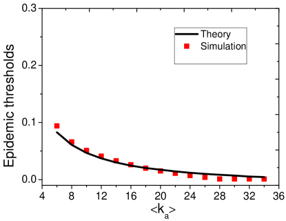
Figure 3: (Color online). Numerical simulation (red square) and theoretical (solid black line) results of epidemic thresholds for the interconnected network versus varying average degree $\langle k_{a}\rangle$.

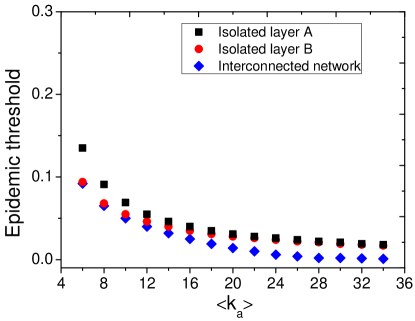
Figure 4: (Color online). Numerical epidemic thresholds as a function of $\langle k_{a}\rangle$ for the interconnected network and the corresponding isolated layers $A$ and $B$.

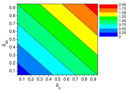
Figure 5: (Color online). Phase diagram of $\Lambda_{\mbox{max}}$ showing the healthy phase ($\Lambda_{\mbox{max}}<1$) and the endemic phase ($\Lambda_{\mbox{max}}>1$) of the interconnected network for the case of $\delta_{a}=\delta_{b}$ and $\delta_{ab}=\delta_{ba}$.

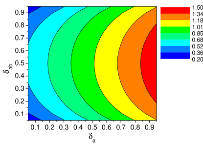
Figure 6: (Color online). Phase diagram showing the healthy phase ($\Lambda_{\mbox{max}}<1$) and the endemic phase ($\Lambda_{\mbox{max}}>1$) of the interconnected network for the case of $\delta_{a}=\delta_{b}$ and $\delta_{ab}=1-\delta_{ba}$.

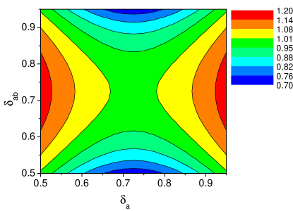
Figure 7: (Color online). Phase diagram of $\Lambda_{\mbox{max}}$ showing the healthy phase ($\Lambda_{\mbox{max}}<1$) and the endemic phase ($\Lambda_{\mbox{max}}>1$) of the interconnected network for the case of $\delta_{a}=1-\delta_{b}$ and $\delta_{ab}=1-\delta_{ba}$.

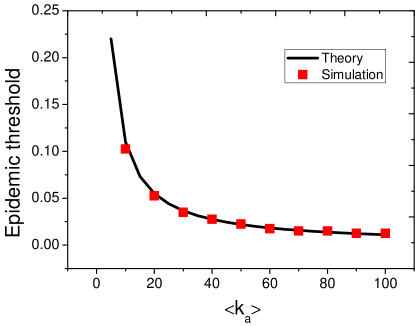
Figure 8: (Color online). Epidemic threshold of the interconnected network (red circum), along with the theoretical prediction (solid black line) based on different average degrees $\langle k_{a}\rangle$.

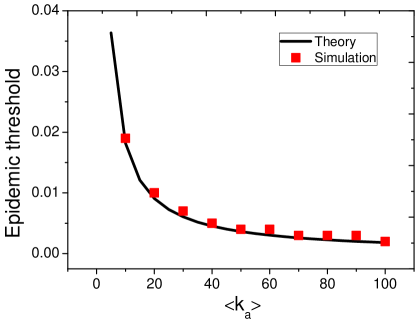
Figure 9: (Color online). Epidemic threshold of the interconnected network (red circum), along with the theoretical prediction (solid black line) based on different average degrees $\langle k_{a}\rangle$.

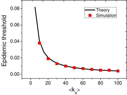
Figure 10: (Color online). Epidemic threshold of the interconnected network (red circum), along with the theoretical prediction (solid black line) based on different average degrees $\langle k_{a}\rangle$.

Figures 8-10 verify Eqs. (25)-(27) for the three specific scenarios. In detail, Fig. 8 shows the result for the case of $\lambda_{ab}\ll\lambda_{a}$, $\langle k_{ab}\rangle<\langle k_{a}\rangle$ and $\langle k_{ba}\rangle<\langle k_{b}\rangle$). It can be seen that the theoretical global epidemic threshold $\lambda^{c}=\frac{1}{k_{max}}$ agrees well with numerical simulations.

Figure 9 shows the result for the scenario with $\lambda_{ab}\approx\lambda_{a},\lambda_{ba}\approx\lambda_{a}$, and $\langle k_{ab}\rangle\approx\langle k_{a}\rangle$, $\langle k_{ba}\rangle\approx\langle k_{b}\rangle$. It can be seen that the theoretical global epidemic threshold $\lambda^{c}=\frac{1}{k_{a}+k_{b}}$ agrees well with numerical results. Figure 10 displays the result for the scenario with $\lambda_{ab}\gg\lambda_{a},\lambda_{ba}\gg\lambda_{a}$, $\langle k_{ab}\rangle>\langle k_{a}\rangle$ and $\langle k_{ba}\rangle>\langle k_{b}\rangle$, which again shows that the theoretical result $\lambda^{c}=\frac{1}{\sqrt{\langle k_{ab}\rangle\langle k_{ba}\rangle}}$ agrees well with numerical simulations. In the three figures, one can see that the epidemic threshold decreases sharply with increasing $\langle k_{a}\rangle$ when $\langle k_{a}\rangle$ is relatively small, then the threshold keeps declining but at a much smaller rate.

III.2 For the two-layered correlated heterogeneous network

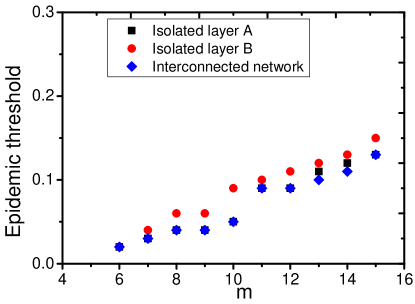
Figure 11: (Color online). Numerical epidemic thresholds as a function of $m$ for two interconnected scale-free networks and the corresponding isolated layers $A$ and $B$ wherein.

Figure 12: (Color online). The epidemic threshold versus the inter-layer degree correlation coefficient $r$ for two interconnected scale-free networks.

Figure 13: (Color online). Total prevalence $\rho$ versus the inter-layer degree correlation coefficient $r$ for two interconnected scale-free networks.

In this sub-section, spreading processes on interconnected BA scale-free networks Barabási and Albert (1999) with inter-layer degree correlation are investigated. The BA algorithm Barabási and Albert (1999) is employed to generate networks for the two layers with identical model parameters but different sizes (i.e., 1000 for layer $A$ and 800 for layer $B$ ). Specifically, start with a fully-connected network of $m0=20$ nodes. At each time step, add a new node, which is connected to $m$ ($m$ is varying) existing nodes with a probability proportional to the number of links that the existing nodes already have.

First, consider the case where the correlation coefficient $r$ for nodes in the two layers is $0$, which means that the two layers are uncorrelated.

In numerical simulations, let $m=(6,7,8,\cdots,15)$ for both layers $A$ and $B$. The comparison of the global epidemic threshold for cooperative interconnected network with the thresholds of the corresponding isolated layers for different scale-free networks are displayed in Fig. 11. It shows that the global epidemic threshold is always lower than those of the corresponding isolated layers, which again verifies that cooperative epidemic spreading on an interconnected network promotes the propagation.

Next, the problem of how the degree correlation between two layers affects the disease spreading dynamics is investigated. For the two scale-free networks, add a fixed number of inter-layer connections (here, the number $\mathcal{L}$ is half of the connections in layer $A$) but with adjustable values of correlation. Specifically, first, connect the two scale-free networks with a random correlation, that is, $r=0$. Then, rewire $\lfloor\mathcal{L}\delta\rfloor$ inter-layer links in such a way that the beginning end is kept and the other end is preferentially reconnected to another node bearing identical or nearly identical degrees so as to yield a larger degree correlation coefficient, where $\delta$ is the rewiring probability. Analogously, rewire $\lfloor\mathcal{L}\delta\rfloor$ inter-layer links in such a way that the beginning end is kept and the other end is preferentially reconnected to another node bearing the most different degree to the beginning end so as to yield a smaller degree correlation coefficient. Obviously, different $\delta$ leads to different correlation coefficients.

For two interconnected $BA$ scale-free networks both with $m=8$, the impact of inter-layer correlation $r$ on the epidemic threshold is shown in Fig. 12. It can be seen that $r$ has little impact on the thresholds. Further, in Fig. 13 the total prevalence $\rho$ as defined in Eq. (44) with varying $r$ is shown for the two scale-free networks, both with $m=8$. It is obvious that the prevalence decreases with increasing $r$, which reveals that when the number of inter-layer connections is half of that in layer $A$, a positive inter-layer node correlation will lead to a drop of total prevalence.

III.3 For the uncorrelated two-layered heterogeneous network

Finally, to compare the epidemic spreading over isolated and interconnected networks, consider two BA scale-free networks, where $m_{0}=10,m=10$ for layer $A$ and $m_{0}=8,m=8$ for layer $B$. Figure 14 shows the total prevalence $\rho^{*}$ defined in Eq. (67) for the two isolated layers $A$ and $B$, with respect to varying parameters $\lambda_{a}$ and $\lambda_{b}$. Figure 15 shows the total prevalence $\rho$ defined in Eq. (51) of the interconnected network. The blue regions ($\rho^{*}=0$ or $\rho=0$) in the lower left part in both figures show that the epidemic is eventually dying out, while other regions ($\rho^{*}>0$ or $\rho>0$) indicate that the epidemic is eventually persistent in the population. The blue region in Fig. 15 for the interconnected network is much smaller than that in Fig. 14 for the isolated layers, which again reveals that epidemic threshold is decreased for cooperative epidemic spreading over the interconnected network. Simultaneously, it can be seen from the different colors that for the same infection rates $\lambda_{a}$ and $\lambda_{b}$, the prevalence for the interconnected network is always larger than that for isolated layers.

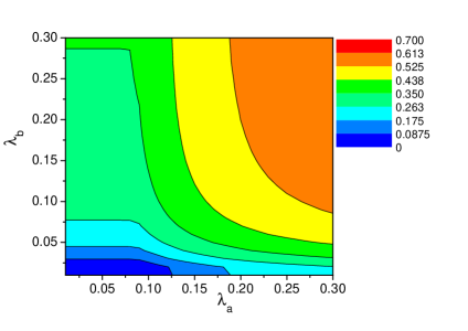
Figure 14: (Color online). Total prevalence $\rho^{*}$ versus infection rates $\lambda_{a}$ and $\lambda_{b}$ for the two isolated layers.

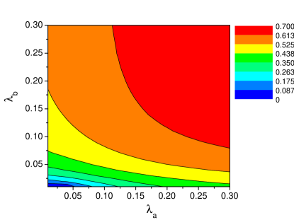
Figure 15: (Color online). Total prevalence $\rho$ versus infection rates $\lambda_{a}$ and $\lambda_{b}$ for the interconnected network.

IV Conclusion

Three models have been formulated to investigate cooperative spreading processes on an interconnected network with or without inter-layer degree correlations. In particular, for an interconnected homogeneous network, the dynamics has been theoretically analyzed at the level of each layer, obtaining global epidemic thresholds from information within each layer and across layers. For an interconnected heterogeneous network with inter-layer correlations, it reveals that inter-layer degree correlation has little impact on the epidemic thresholds, but a larger inter-layer degree correlation coefficient leads to a smaller total prevalence. The global epidemic threshold is determined by the maximum eigenvalues of supra-connectivity matrix and supra-adjacency marix for correlated and uncorrelated networks, respectively. It was found that, the epidemic thresholds of spreading processes are decreased for interconnected networks, implying that cooperative spreading processes promote the spread of diseases. The results may provide references to public health monitoring for disease control and prevention.

References

• Pastor-Satorras and Vespignani (2001) R. Pastor-Satorras and A. Vespignani, Physical Review E 63, 138 (2001).
• Newman (2002) M. E. J. Newman, Physical Review E 66, 016128 (2002).
• Motter et al. (2002) A. E. Motter, T. Nishikawa,  and Y. C. Lai, Physical Review E 66, 065103 (2002).
• Eames and Keeling (2004) K. T. D. Eames and M. J. Keeling, Mathematical Biosciences 189, 115 (2004).
• Liljeros et al. (2003) F. Liljeros, C. R. Edling,  and L. A. N. Amaral, Microbes & Infection 5, 189 (2003).
• Reed (2006) W. J. Reed, Mathematical Biosciences 201, 3 (2006).
• Saumell-Mendiola et al. (2012) A. Saumell-Mendiola, M. . Serrano,  and M. Bogu? , Physical Review E 86, 026106 (2012).
• Dickison et al. (2012) M. Dickison, S. Havlin,  and H. E. Stanley, Physical Review E 85, 066109 (2012).
• Yagan et al. (2013) O. Yagan, D. Qian, J. Zhang,  and D. Cochran, IEEE Journal on Selected Areas in Communications 31, 1038 (2013).
• Domenico et al. (2013) M. D. Domenico, A. Sol$\grave{e}$ribalta, E. Cozzo, M. Kivel, Y. Moreno, M. A. Porter, S. G$\grave{o}$mez,  and A. Arenas, Physical Review X 3, 041022 (2013).
• Zhao et al. (2014a) D. Zhao, L. Li, H. Peng, Q. Luo,  and Y. Yang, Physics Letters A 378, 770 (2014a).
• Xu et al. (2015) M. Xu, J. Zhou, J. A. Lu,  and X. Wu, The European Physical Journal B 88, 1 (2015).
• Li et al. (2015) Y. Li, X. Wu, J.-A. Lu,  and J. L , IEEE Transactions on Circuits and Systems II: Express Briefs 63, 1 (2015).
• Cozzo et al. (2013) E. Cozzo, R. A. Ba$\tilde{n}$os, S. Meloni,  and Y. Moreno, Physical Review E 88, 050801 (2013).
• Wang et al. (2013) H. Wang, Q. Li, G. D’Agostino, S. Havlin, H. E. Stanley,  and P. V. Mieghem, Physical Review E 88, 279 (2013).
• Sanz et al. (2014) J. Sanz, C. Y. Xia, S. Meloni,  and Y. Moreno, Physical Review X 4, 041005 (2014).
• Clara et al. (2013) G. Clara, G. Sergio,  and A. Alex, Physical Review Letters 111, 1 (2013).
• Granell et al. (2014) C. Granell, S. Gomez,  and A. Arenas, Physical Review E 90, 012808 (2014).
• Lee et al. (2012) K. M. Lee, J. Y. Kim, W. Cho, K. I. Goh,  and I. M. Kim, New Journal of Physics 14, 033027 (2012).
• Barigozzi et al. (2009) M. Barigozzi, G. Fagiolo,  and D. Garlaschelli, Physical Review E 81, 046104 (2009).
• Parshani et al. (2011) R. Parshani, C. Rozenblat, D. Ietri, C. Ducruet,  and S. Havlin, EPL 92, 2470 (2011).
• Xu et al. (2011) X. L. Xu, Y. Q. Qu, S. Guan, Y. M. Jiang,  and D. R. He, EPL 93, 3437 (2011).
• Buldyrev et al. (2011) S. V. Buldyrev, N. W. Shere,  and G. A. Cwilich, Physical Review E 83, 016112 (2011).
• Nicosia and Latora (2015) V. Nicosia and V. Latora, Physical Review E 92, 032805 (2015).
• Wang et al. (2014) W. Wang, M. Tang, H. Yang, Y. Do, Y. C. Lai,  and G. Lee, Scientific Reports 4, 5097 (2014).
• Tanaka (2012) G. Tanaka, Scientific Reports 2, 232 (2012).
• Bapat (2010) R. B. Bapat, Graphs and Matrices (Springer London, 2010) pp. 125–140.
• Morens et al. (2004) D. M. Morens, G. K. Folkers,  and A. S. Fauci, Nature 430, 242 (2004).
• Watts and Strogatz (1998) D. J. Watts and S. H. Strogatz, Nature 6684, 440 (1998).
• Barabási and Albert (1999) A.-L. Barabási and R. Albert, Science 286, 509 (1999).
• Vida et al. (2015) R. Vida, J. Galeano,  and S. Cuenda, Physica A 421, 134 (2015).
• Gomez et al. (2010) S. Gomez, A. Arenas, J. Borge-Holthoefer, S. Meloni,  and Y. Moreno, EPL 89, 275 (2010).
• Zhao et al. (2014b) Y. Zhao, M. Zheng,  and Z. Liu, Chaos 24, 043129 (2014b).
• Jun et al. (2013) T. Jun, R. Yuhua, Y. Lu, S. H. Vermund, B. E. Shepherd, S. Yiming,  and Q. Han-Zhu, Aids Patient Care & Stds 27, 524 (2013).
• Van et al. (2013) G. C. Van, K. Vongsaiya, C. Hughes, R. Jenkinson, A. L. Bowring, A. Sihavong, C. Phimphachanh, N. Chanlivong, M. Toole,  and M. Hellard, Aids Education & Prevention Official Publication of the International Society for Aids Education 25, 232 (2013).
• Bauch and Galvani (2013) C. T. Bauch and A. P. Galvani, Science 342, 47 (2013).
• Liljeros et al. (2001) . Liljeros, F., C. R. Edling, L. A. Amaral, H. E. Stanley,  and . Aberg, Y., Nature 411, 907 (2001).
• Vespignani (2000) P. S. A. Vespignani, Physical Review Letters 86, 3200 (2000).
• Egu$\acute{i}$luz and Konstantin (2002) V. M. Egu$\acute{i}$luz and K. Konstantin, Physical Review Letters 89, 108701 (2002).
• Mari$\acute{a}$et al. (2003) B. Mari$\acute{a}$n, P. S. Romualdo,  and V. Alessandro, Physical Review Letters 90, 028701 (2003).
• Bogu$\tilde{n}$ $\acute{a}$ and Pastor-Satorras (2002) M. Bogu$\tilde{n}$ $\acute{a}$ and R. Pastor-Satorras, Physical Review E 66, 107 (2002).
• Vittoria and Alessandro (2007) C. Vittoria and V. Alessandro, Physical Review Letters 99, 12243 (2007).
• Colizza et al. (2007) V. Colizza, R. Pastor-Satorras,  and A. Vespignani, Nature Physics 3, 276 (2007).
• Colizza and Vespignani (2008) V. Colizza and A. Vespignani, Journal of Theoretical Biology 251, 450 (2008).
• Baronchelli et al. (2008) A. Baronchelli, M. Catanzaro,  and R. Pastor-Satorras, Physical Review E 78, 016111 (2008).
• Tang et al. (2009) M. Tang, Z. Liu,  and B. Li, EPL 87 (2009).
• Liu (2010) Z. Liu, Physical Review E 81, 016110 (2010).
• Buscarino et al. (2007) A. Buscarino, L. Fortuna, M. Frasca,  and V. Latora, EPL 82, 283 (2007).
• Zhou and Liu (2009) J. Zhou and Z. Liu, Physica A 388, 1228 (2009).
• Funk and Jansen (2010) S. Funk and V. A. A. Jansen, Physical Review E 81, 417 (2010).
• Guo et al. (2015) Q. Guo, X. Jiang, Y. Lei, M. Li, Y. Ma,  and Z. Zheng, Phys.rev.e 91 (2015).
• Sahneh and Scoglio (2014) F. D. Sahneh and C. Scoglio, Physical Review E 89, 1 (2014).
• Ruan et al. (2013) Z. Ruan, P. Hui, H. Lin,  and Z. Liu, The European Physical Journal B - Condensed Matter and Complex Systems 86, 1 (2013).
• Aguirre et al. (2014) J. Aguirre, R. Sevilla-Escoboza, R. Gutiérrez, D. Papo,  and J. Buldú, Physical Review Letters 112, 248701 (2014).
• De Domenico et al. (2013) M. De Domenico, A. Solé, S. Gómez,  and A. Arenas, arXiv preprint arXiv:1306.0519  (2013).
• Erd6s and Rényi (1960) P. Erd6s and A. Rényi, Publ. Math. Inst. Hungar. Acad. Sci 5, 17 (1960).
• Gómez-Gardenes et al. (2012) J. Gómez-Gardenes, I. Reinares, A. Arenas,  and L. M. Floría, Scientific reports 2 (2012).
• Gomez et al. (2013) S. Gomez, A. Diaz-Guilera, J. Gomez-Gardeñes, C. J. Perez-Vicente, Y. Moreno,  and A. Arenas, Physical review letters 110, 028701 (2013).
• Pluchino et al. (2006) A. Pluchino, V. Latora,  and A. Rapisarda, The European Physical Journal B-Condensed Matter and Complex Systems 50, 169 (2006).
• Radicchi and Arenas (2013) F. Radicchi and A. Arenas, Nature Physics 9, 717 (2013).
• Wu et al. (2009) X. Wu, W. X. Zheng,  and J. Zhou, Chaos 19, 193 (2009).