Kagome-like chains with anisotropic ferromagnetic and antiferromagnetic interactions

Abstract

We consider a spin-$\frac{1}{2}$ kagome-like chain with competing ferro- and antiferromagnetic anisotropic exchange interactions. The ground state phase diagram of this model consists of the ferromagnetic and ferrimagnetic phases. We study the ground state and the low-temperature properties on the phase boundary between these phases. The ground state on this phase boundary is macroscopically degenerate and consists of localized magnon states. We calculate the ground state degeneracy and corresponding residual entropy. The spontaneous magnetization has a jump on the phase boundary confirming the first-order type of the phase transition. In the limit of a strong anisotropy the spectrum of the low-energy excitations has multi-scale structure governing the peculiar features of the specific heat behavior.

I Introduction

The low-dimensional quantum magnets on geometrically frustrated lattices have been extensively studied during last years diep ; mila . There is a broad class of highly frustrated antiferromagnetic spin systems which supports a completely dispersionless magnon band (flat band) flat ; shulen ; zhit ; mak so that the excitations in this band are localized states. The localization of the one-magnon states is a base for the construction of multi-magnon states, because a state consisting of independent (non-overlapping) localized magnons is an exact eigenstate. Such systems include, for example, the delta-chain, the kagome lattice, kagome-like chains, the Tasaki lattice etc. An important feature of them is the triangular geometry of antiferromagnetic bonds. Besides, for these models a special condition of flat band is required. For example, for the delta chain (Fig.1) the relation between interactions must be $J_{2}=\frac{1}{2}J_{1}$. It was found flat that the ground states of such systems at the saturation magnetic field consist of independent localized magnons. The ground state and low-temperature properties for the antiferromagnetic Heisenberg models with flat band have been actively studied over last decades. It was shown that flat band physics may lead to new interesting phenomena such as the residual entropy at the saturation magnetic field, the zero-temperature magnetization plateau and the magnetization jump, an extra low-temperature peak in the specific heat etc. schmidt ; honecker ; zhitomir ; Derzhko ; zhit .

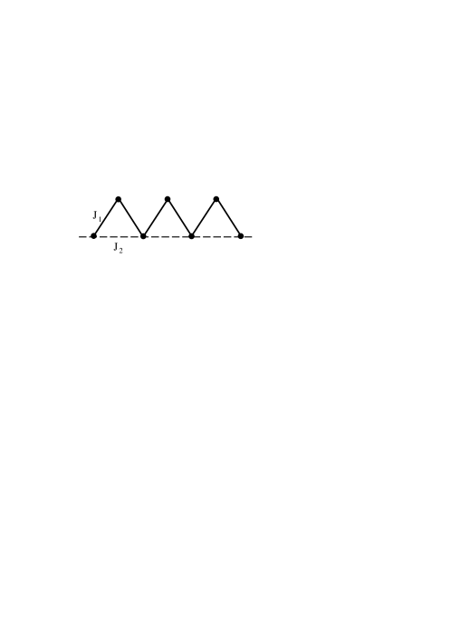
Figure 1: The delta-chain model.

Recently it was found that the localized magnon states can be supported in a certain frustrated spin system with competing ferro- (F) and antiferromagnetic (AF) interactions. This model is the $s=\frac{1}{2}$ delta-chain Heisenberg model with the ferromagnetic $J_{1}<0$ and the antiferromagnetic $J_{2}>0$ interactions (F-AF delta-chain). For $J_{2}=-\frac{J_{1}}{2}$ the localized states exist in this model. However, in contrast with the AF-AF delta-chain the localized magnon states of the F-AF chain are exact ground states at zero magnetic field. Besides, the ground state manifold contains the special states with overlapping magnons (localized multimagnon complexes). So, the ground state degeneracy in this model is even higher than for AF-AF delta chain. The properties of such F-AF delta chain have been studied in Ref.KDNDR ; anis .

In this paper we will study another example of frustrated spin $s=\frac{1}{2}$ model with ferro- and antiferromagnetic interactions. It is a kagome-like chain consisting of a linear chain of corner sharing triangular plaquettes as shown in Fig.2. The interaction $J_{1}$ between leg and axis spins is ferromagnetic ($J_{1}<0$). The interaction $J_{2}$ acts between nearest spins on the same leg, while $J_{3}$ is the interaction between spins on opposite legs. Both interactions $J_{2}$ and $J_{3}$ are antiferromagnetic. We will consider two versions of kagome-like chains, denoted as $(a)$ and $(b)$. In the model $(a)$ the interaction $J_{3}=0$ and we denote the interaction $J_{2}$ as $J_{2}=J_{a}$. In the model $(b)$ the interactions between nearest spins on both the same and the opposite legs are equal and $J_{2}=J_{3}=J_{b}$. The Hamiltonians of these F-AF kagome-like chains have the forms:

$$\hat{H}=\sum_{i=1}^{n}\hat{H}_{i}$$ (1)

where $\hat{H}_{i}$ is the Hamiltonian of the $i$-th pair of corner sharing triangles (pair of triangles for brevity) and $\hat{H}_{i}$ for the kagome-chains $(a)$ and $(b)$ have the forms

$$\hat{H}_{ia} = -\sum_{\nu=x,y}(\sigma_{i}^{\nu}+\sigma_{i+1}^{\nu}+\xi_{i}^{\nu}+\xi_{i+1}^{\nu})s_{i}^{\nu}+\Delta_{1}[(\sigma_{i}^{z}+\sigma_{i+1}^{z}+\xi_{i}^{z}+\xi_{i+1}^{z})s_{i}^{z}-1]$$ (2)

$$+J_{a}\sum_{\nu=x,y}(\sigma_{i}^{\nu}\sigma_{i+1}^{\nu}+\xi_{i}^{\nu}\xi_{i+1}^{\nu})+\Delta_{2}(\sigma_{i}^{z}\sigma_{i+1}^{z}+\xi_{i}^{z}\xi_{i+1}^{z}-\frac{1}{2})$$

$$\hat{H}_{ib} = -\sum_{\nu=x,y}(\sigma_{i}^{\nu}+\xi_{i}^{\nu}+\sigma_{i+1}^{\nu}+\xi_{i+1}^{\nu})s_{i}^{\nu}+\Delta_{1}[(\sigma_{i}^{z}+\xi_{i}^{z}+\sigma_{i+1}^{z}+\xi_{i+1}^{z})s_{i}^{z}-1]\}$$ (3)

$$+J_{b}\sum_{\nu=x,y}(\sigma_{i}^{\nu}+\xi_{i}^{\nu})(\sigma_{i+1}^{\nu}+\xi_{i+1}^{\nu})+\Delta_{2}[(\sigma_{i}^{z}+\xi_{i}^{z})(\sigma_{i+1}^{z}+\xi_{i+1}^{z})-1]\}$$

where $s_{i}^{\nu}$, $\sigma_{i}^{\nu}$ and $\xi_{i}^{\nu}$ are $s=\frac{1}{2}$ operators of spins on axis, lower and upper leg sites, respectively. $J_{a}$ and $J_{b}$ are the antiferromagnetic leg-leg interactions and we put $J_{1}=-1$. $\Delta_{1}$ and $\Delta_{2}$ are parameters representing the anisotropy of the axis-leg and the leg-leg exchange interactions respectively, $n$ is the number of axis sites. The periodic boundary conditions (PBC) are imposed. The constants in Eqs.(2) and (3) are chosen so that the energy of the ferromagnetic state with the total spin of the system $L^{z}=\pm\frac{3n}{2}$ is zero. As it is seen from Eq.(3) for the model $(b)$ the spins on the upper and lower legs present in the Hamiltonian only in the combinations $(\sigma_{i}^{\nu}+\xi_{i}^{\nu})$ $(\nu=x,y,z)$, effectively forming the composite spin of pair $(\vec{\sigma}_{i}+\vec{\xi}_{i})$ which can be either 0 or 1.

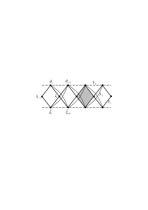
Figure 2: The kagome-like spin chain model.

The ground state and the low-temperature properties of the isotropic Heisenberg model on the kagome chain Fig.2 with the antiferromagnetic interactions $J_{1},J_{2}>0$ and $J_{3}=0$ has been studied as a function of parameter $\frac{J_{2}}{J_{1}}$ in Ref.wald . At $\frac{J_{2}}{J_{1}}<\frac{1}{2}$ the ground state is ferrimagnetic of the Lieb-Mattis type lieb and at $\frac{J_{2}}{J_{1}}>\frac{1}{2}$ it is the singlet. This model with $J_{2}=J_{1}$ belongs to the class of the flat band models with multi-magnon states consisting of independent localized magnons. The ground state and the low-temperature properties of such AF-kagome-chain with $J_{1}=J_{2}$ have been studied in detail in Refs.schnack ; honecker .

In contrast to the antiferromagnetic kagome-chain the models with the leg-axis ferromagnetic and leg-leg antiferromagnetic interactions ($J_{1}<0$ and $J_{a}$, $J_{b}>0$) (F-AF kagome-chains) are less studied. The isotropic kagome-chain $(b)$ with $\Delta_{1}=\Delta_{2}=1$ is especially interesting because it is a minimal model for a description of an interesting class of quasi-one-dimensional compounds $\mathrm{Ba_{3}Cu_{3}In_{4}O_{12}}$ and $\mathrm{Ba_{3}Cu_{3}Sc_{4}O_{12}}$ vasil ; soos1 ; soos ; vasiliev ; indus and the form of the Hamiltonian $\hat{H}_{b}$ reflects an unusual topology of these copper oxides. These oxides represent half-twist ladders in which successive $\mathrm{CuO}_{4}$ plaquettes are corner shared with their planes perpendicular to each other. The dominant interaction in these compounds is between the leg and the axis spins and it is ferromagnetic vasil ; soos1 ; soos ; vasiliev ; indus . Though the values of the antiferromagnetic leg-leg interactions are not known definitely it is expected that they are rather small in comparison with $J_{1}$. It means that probably $J_{b}\ll 1$ in these compounds. Nevertheless, the study of the influence of the interaction $J_{b}$ on the properties of this model is important problem. Besides, both F-AF kagome-chains are interesting spin systems in its own right.

The ground state phase diagram of the isotropic F-AF kagome models can be analyzed with using of the one-magnon spectrum or the classical approximation. For example, the minimal energy of one-magnon excitations over the ferromagnetic state is positive for $J_{a}<\frac{1}{2}$ ($J_{b}<\frac{1}{4}$) and negative for $J_{a}>\frac{1}{2}$ ($J_{b}>\frac{1}{4}$). Our numerical calculations have shown that for $J_{a}>\frac{1}{2}$ ($J_{b}>\frac{1}{4}$) the ground state is ferrimagnetic. The critical points $J_{a}=\frac{1}{2}$ and $J_{b}=\frac{1}{4}$ are the transition points between these two ground state phases. As will be shown the F-AF kagome chains have exact localized states at the transition points $J_{a}=\frac{1}{2}$ ($J_{b}=\frac{1}{4}$). However, similarly to the F-AF delta chain in addition to the multi-magnon configurations consisting of isolated magnons the special states with overlapping magnons (localized multi-magnon complex) exist and all of them are exact ground states at zero magnetic field. The ground state degeneracy in F-AF kagome-chain is macroscopic and higher than for the antiferromagnetic kagome chain with $J_{2}=J_{1}$. It turns out that such degeneracy is not exceptional property of the isotropic F-AF kagome chains and it exists also in the more general F-AF model with anisotropic exchange interactions for definite relations between them. The Hamiltonians of such anisotropic models depend on a single parameter which can be taken as the anisotropy of the leg-axial interaction $\Delta_{1}$. These models describe the phase boundary (a transition line) between different ground state phases on the ($J_{a,b}$, $\Delta_{1}$) planes: the ferromagnetic phase at $J_{a}<\frac{1}{2\Delta_{1}}$, $J_{b}<\frac{1}{4\Delta_{1}}$ and the ferrimagnetic phase at $J_{a}>\frac{1}{2\Delta_{1}}$, $J_{b}>\frac{1}{4\Delta_{1}}$. The ground state degeneracy on this line does not depend on $\Delta_{1}$ and grows exponentially with the system size giving rise to a residual zero-temperature entropy. In the limiting case $\Delta_{1}=\infty$ the models turn into the Ising models on the kagome-chains.

The main aim of this paper is to study the F-AF kagome-chains on the transition line. We will demonstrate that the behavior of the model on this line has non-trivial peculiarities depending on $\Delta_{1}$. The limit of the large anisotropy $\Delta_{1}$ is especially interesting. In this limit the spectrum of low-energy excitations has a multi-scale structure. This peculiarity of the spectrum induces the specific properties of the low-temperature thermodynamics. In particular, the specific heat has many low-temperature peaks. When the anisotropy $\Delta_{1}$ decreases the spectrum of excitations is gradually smeared and flattening of the peaks occurs. In the isotropic case $\Delta_{1}=1$ one low-temperature maximum in $C(T)$ dependence survives in model $(a)$ while it transforms to a shoulder in model $(b)$.

In many respects the properties of the kagome-like chains on the transition line are similar to those for the F-AF delta-chain studied in Refs.KDNDR ; anis . Therefore, we will refer to KDNDR ; anis for the technical details.

The paper is organized as follows. In section II we study the ground state properties of the F-AF kagome chains on the transition line. In section III we study the kagome chains with large anisotropy $\Delta_{1}$ including the Ising limit. The structure of the spectrum of low-energy excitations and their influence on the behavior of the specific heat will be studied. The properties of the isotropic kagome chains in the transition point is considered in section IV. In section V we give a summary of our results.

II Ground state degeneracy

In this section we study the ground state of the F-AF kagome chains on the phase boundary between the ferromagnetic and ferrimagnetic phases. At first, we consider the one-magnon states, i.e. the states in the spin sector $L^{z}=L_{\max}^{z}-1$ ($L_{\max}^{z}=\frac{3n}{2}$), where we define the total spin as $\vec{L}=\sum_{i}(\vec{s}_{i}+\vec{\sigma}_{i}+\vec{\xi}_{i})$ and denote the quantum number of its magnitude and the z-component by $L$ and $L^{z}$, respectively. The primitive unit cell of the kagome chain contains three sites. The corresponding three branches of one-magnon states with $L^{z}=L_{\max}^{z}-1$ have the energies:

$$E_{\pm}(q) = \frac{1}{2}\left[(3\Delta_{1}-J_{a,b}(\Delta_{2}+\cos q)\pm\sqrt{(\Delta_{1}+J_{a,b}(\Delta_{2}-\cos q)^{2}+4(1+\cos q)}\right]$$

$$E_{3a}(q) = J_{a}\cos q+\Delta_{1}-J_{a}\Delta_{2},\quad E_{3b}(q)=\Delta_{1}-2J_{b}\Delta_{2}$$ (4)

where $\alpha=J_{a}$ for model $(a)$ and $\alpha=2J_{b}$ for model $(b)$.

If we choose exchange interactions as

$$J_{a} = \frac{1}{2\Delta_{1}},\quad\Delta_{2}=2\Delta_{1}^{2}-1$$

$$J_{b} = \frac{1}{4\Delta_{1}},\quad\Delta_{2}=2\Delta_{1}^{2}-1$$ (5)

then the lowest band becomes flat with zero energy, $E_{-}(q)=0$. For the isotropic model the lowest band is flat if $J_{a}=\frac{1}{2}$ and $J_{b}=\frac{1}{4}$ for $(a)$ and $(b)$ models, respectively. The energy of the second branch is positive for all $q$ ($E_{+}(q)\geq 2\Delta_{1}$). The third band for the model $(a)$ becomes $E_{3a}=(1+\cos q)/2\Delta_{1}$ and approaches to zero at $q=\pi$, providing an additional one-magnon state with zero energy to $n$ states of the lowest band. For the model $(b)$ the third band is flat with the positive energy $E_{3b}(q)=\frac{1}{2\Delta_{1}}$.

The dispersionless one-magnon states of lowest band correspond to localized states which can be chosen for both models $(a)$ and $(b)$ as

$$\hat{\varphi}_{i}\left|F\right\rangle=[s_{i}^{-}+s_{i+1}^{-}+2\Delta_{1}(\sigma_{i}^{-}+\xi_{i}^{-})]\left|F\right\rangle\quad i=1,\ldots n$$ (6)

where $\left|F\right\rangle$ is the ferromagnetic state with all spins up, $s_{i}^{-},\sigma_{i}^{-},\xi_{i}^{-}$ are spin lowering operators.

In the isotropic case the wave function of the localized magnon is

$$\hat{\varphi}_{i}\left|F\right\rangle=[s_{i}^{-}+s_{i+1}^{-}+2(\sigma_{i}^{-}+\xi_{i}^{-})]\left|F\right\rangle\quad i=1,\ldots n$$ (7)

The wave function $\hat{\varphi}_{i}\left|F\right\rangle$ is localized in a diamond with shaded area in Fig.2. It can be checked directly that the functions (6) are exact eigenfunction with zero energy of each local Hamiltonian $\hat{H}_{ia,b}$ (Eqs.(2),(3)) with exchange interactions satisfying conditions (5) and, therefore, of the total Hamiltonian (1). All $n$ states (6) are linear independent KDNDR . For the model $(a)$ there is in addition another linear independent exact wave function with zero energy. It is non-localized one and it has a form

$$\hat{\phi}\left|F\right\rangle=\sum_{i=1}^{n}(-1)^{i}(\sigma_{i}^{-}-\xi_{i}^{-})\left|F\right\rangle$$ (8)

Thus, the ground state energy in the spin sector $L^{z}=L_{\max}^{z}-1$ is zero and there are $n$ or $(n+1)$ such states for the kagome-chains $(b)$ or $(a)$. In the isotropic case the operator $\vec{L}$ commutes with the Hamiltonian (1) and there are $(n-1)$ linear combinations of $\hat{\varphi}_{i}\left|F\right\rangle$ which belong to the states with $L=L_{\max}-1$ and one combination belongs to $L=L_{\max}$. The latter is

$$\sum\hat{\varphi}_{i}\left|F\right\rangle=2L_{tot}^{-}\left|F\right\rangle.$$ (9)

The non-localized wave function (8) in the model $(a)$ belong to $L=L_{\max}-1$.

The ground state energy in any spin sector can not be negative. This statement can be proved by a standard way. At first, it can be checked that 16 eigenvalues of $\hat{H}_{ia}$ and 10 eigenvalues of $\hat{H}_{ib}$ are zero. All other eigenvalues of $\hat{H}_{ia}$ and $\hat{H}_{ib}$ are positive. Thus, the ground state energy $E_{0}$ of $\hat{H}$ satisfies an inequality $E_{0}\geq 0$. This inequality turns in an equality for the ground states in the spin sectors $L^{z}=L_{\max}^{z}$ and $L^{z}=L_{\max}^{z}-1$. The question is: how many states in other spin sectors have zero energy?

Let us consider the ground state in the spin spin sector $L^{z}=L_{\max}^{z}-2$ (two-magnon states). It is evident that the pairs of the independent (isolated) magnons $\hat{\varphi}_{i}\hat{\varphi}_{j}\left|F\right\rangle$ ($\left|i-j\right|>1$) are the eigenfunctions with zero energy of each local Hamiltonian (and, therefore, of total Hamiltonian) in this spin sector. However, such states do not exhaust all possible ones with zero energy. For example, we can write in the isotropic case the exact two-magnon state as

$$(\hat{\varphi}_{i-1}+\hat{\varphi}_{i}+\hat{\varphi}_{i+1})\hat{\varphi}_{i}\left|F\right\rangle$$ (10)

The wave function (10) is exact one with zero energy because

$$(\hat{\varphi}_{i-1}+\hat{\varphi}_{i}+\hat{\varphi}_{i+1})\hat{\varphi}_{i}\left|F\right\rangle=2L_{tot}^{-}\hat{\varphi}_{i}\left|F\right\rangle-\sum_{\left|i-j\right|>1}\hat{\varphi}_{j}\hat{\varphi}_{i}\left|F\right\rangle$$ (11)

and both function in the right hand of Eq.(11) are the exact wave functions with zero energy. We note that the function (10) contains overlapping magnons. It can be shown that pairs of isolated magnons and $n$ eigenfunctions (10) are linearly independent KDNDR . Thus, for the model $(b)$ the complete manifold of ground states in the sector $L^{z}=L_{\max}^{z}-2$ consists of $\frac{n(n-3)}{2}$ pairs of isolated magnons and $n$ eigenfunctions (10) so the ground state degeneracy in this spin sector is $C_{n}^{2}$. However, for the model $(a)$ there are also two additional exact two-magnon non-localized wave functions with zero energy. One of them is

$$\hat{\varphi}_{\sigma}\hat{\varphi}_{\xi}\left|F\right\rangle$$ (12)

where

$$\hat{\varphi}_{\sigma(\xi)}=\sum_{i=1}^{n}(-1)^{i}\sigma^{-}(\xi^{-})$$ (13)

and another function is $L_{\mathrm{tot}}^{-}\hat{\phi}\left|F\right\rangle$. The ground state degeneracy of the model $(a)$ in the spin sector $L^{z}=L_{\max}^{z}-2$ is $C_{n}^{2}+2$.

The two-magnon wave function of type (10) can be written also for the anisotropic model with exchange interactions (5). It has a form

$$\hat{\varphi}_{i}(\hat{\varphi}_{i-1}+B\hat{\varphi}_{i}+\hat{\varphi}_{i+1})\left|F\right\rangle$$ (14)

where $B=2\Delta_{1}^{2}-1$ and the degeneracy of the ground state for the models $(a)$ and $(b)$ is the same as for the isotropic model.

It is evident that eigenfunctions composed of $k$ isolated magnons are the exact eigenfunction of the ground state in the spin sector $L^{z}=\frac{3}{2}n-k$. In addition, the construction of the wave functions of type (10) can be extended for $k>2$. Analysis similar to that for the F-AF delta-chain KDNDR shows that total number of the exact ground states functions, $G_{n}(k)$, for fixed $L^{z}=L_{\max}^{z}-k$ is

$$G_{na}(1) = C_{n}^{1}+1$$

$$G_{na}(k) = C_{n}^{k}+2,\qquad 2\leq k\leq\frac{n}{2}$$

$$G_{na}(k) = C_{n}^{n/2}+2,\qquad\frac{n}{2}<k\leq\frac{3n}{2}$$ (15)

$$G_{nb}(k) = C_{n}^{k},\qquad 0\leq k\leq\frac{n}{2}$$

$$G_{nb}(k) = C_{n}^{n/2},\qquad\frac{n}{2}<k\leq\frac{3n}{2}$$ (16)

The total degeneracy of the ground state $W$ is

$$W_{a} = 2^{n}+2nC_{n}^{n/2}+3n+1$$

$$W_{b} = 2^{n}+2nC_{n}^{n/2}$$ (17)

We note that the degeneracy of the ground state given by Eqs.(15) and (16) is valid for any $\Delta_{1}$ on the transition line. Eqs.(15) and (16) have been confirmed by an exact diagonalization of finite kagome chains up to $N=24$.

According to Eqs.(17) the degeneracy of the ground state of the kagome-chains on the transition line is exponentially large. It leads to the residual entropy $s_{0}=\ln(W)/N$ ($N=3n$). In the thermodynamic limit $N\to\infty$ the residual entropy is the same for both kagome-chain models and it is equal to

$$s_{0}=\frac{1}{3}\ln 2$$ (18)

Thus, the entropy per spin is finite at $T=0$. Another unusual property of the macroscopic degenerate ground state is the existence of the non-zero spontaneous magnetization at $T\to 0$. To show this we calculate the contribution to the partition function from only the degenerate ground states. Using Eqs.(15) and (16) we represent such truncated partition function $Z_{gs}$ of the kagome chains in the magnetic field $h$ in a form KDNDR

$$Z_{gs}=2\sum_{k=0}^{n/2}C_{n}^{k}\cosh\left[\frac{(\frac{3}{2}n-k)h}{T}\right]+2C_{n}^{n/2}\sum_{k=0}^{n/2}\cosh\left[\frac{(\frac{3}{2}n-k)h}{T}\right]$$ (19)

The magnetization is given by $M=T(d\ln Z/dh)$. Using steepest descent method for calculation of $Z$ we obtain the expression for the magnetization at $N\gg 1$ in a form

$$\frac{M}{N}=\frac{1+3\exp(h/T)}{6+6\exp(h/T)}$$ (20)

At $\frac{h}{T}\to 0$ the spontaneous magnetization is $\frac{M}{N}=\frac{1}{3}$. It means that the ground state is magnetically ordered.

III Kagome chains with high anisotropy

In this section we study the low-temperature properties of the anisotropic F-AF kagome-chains on the transition line. At first we consider the limit of large $\Delta_{1}$. At $\Delta_{1}\to\infty$ models (2) and (3) reduce to the Ising models on kagome-chains, the Hamiltonians of which are

$$\hat{H}_{Ia} = -\sum_{i}[s_{i}^{z}(\sigma_{i-1}^{z}+\sigma_{i}^{z}+\xi_{i-1}^{z}+\xi_{i}^{z})-1]+\sum_{i}(\sigma_{i}^{z}\sigma_{i+1}^{z}+\xi_{i}^{z}\xi_{i+1}^{z}-\frac{1}{2})-h\sum_{i}(s_{i}^{z}+\sigma_{i}^{z}+\xi_{i}^{z})$$

$$\hat{H}_{Ib} = \hat{H}_{Ia}-\frac{1}{2}\sum_{i}(\sigma_{i}^{z}-\xi_{i}^{z})(\sigma_{i+1}^{z}-\xi_{i+1}^{z})$$ (21)

where $h$ is a dimensionless magnetic field and the F and the AF interactions in $\hat{H}_{Ia}$ are equal in magnitude while in $\hat{H}_{Ib}$ the AF interaction is half of the F interaction.

The partition function of these Ising models can be obtained using a transfer-matrix method and it is given by

$$Z=\lambda_{1}^{n}+\lambda_{2}^{n}+\lambda_{3}^{n}+\lambda_{4}^{n}$$ (22)

where eigenvalues of the transfer matrix $\lambda_{i}$ for the model $\hat{H}_{Ia}$ and $\hat{H}_{Ib}$ for $T\ll 1$ are solutions of equations

$$\left[\lambda^{3}-4\lambda^{2}\cosh\left(\frac{h}{T}\right)\cosh\left(\frac{h}{2T}\right)-\lambda-2\lambda\cosh\left(\frac{2h}{T}\right)+2\cosh\left(\frac{3h}{2T}\right)\right]\times$$

$$\times\left[\lambda+2\cosh\left(\frac{h}{2T}\right)\right]=0$$ (23)

for the model $(a)$ and

$$\lambda\left[\lambda^{3}-2\lambda^{2}\cosh\left(\frac{3h}{2T}\right)-4\lambda\cosh\left(\frac{2h}{T}\right)+4\lambda\cosh^{2}\left(\frac{h}{2T}\right)+\lambda-4\cosh\left(\frac{h}{2T}\right)\right]=0$$ (24)

for the model $(b)$.

The eigenvalues $\lambda_{i}$ at $h/T=0$ are

$$\lambda_{1,2a} = \frac{5\pm\sqrt{17}}{2},\quad\lambda_{3a}=-1,\quad\lambda_{4a}=-2$$

$$\lambda_{1b} = 4,\quad\lambda_{2b}=\lambda_{3b}=-1,\quad\lambda_{4b}=0$$ (25)

The ground state of models (21) at $h=0$ has zero energy and excited states are separated by a gap $\Delta E\simeq 1$. The ground state is macroscopically degenerate and the total ground state degeneracy $W$ at $n\gg 1$ is defined by the largest eigenvalues of (25)

$$W_{a} = (\frac{5+\sqrt{17}}{2})^{n}\simeq 4.56^{n}$$

$$W_{b} = 4^{n}$$

We note that the ground state degeneracy is different for the model $\hat{H}_{Ia}$ and $\hat{H}_{Ib}$.

The ground state degeneracies $G_{In}(k)$ in the spin sector $L^{z}=(\frac{3n}{2}-k)$ ($0\leq k\leq\frac{3n}{2}$) can be found as coefficients in the expansion of a partition function $Z/\exp(\frac{3hn}{2T})$ in powers of $\exp(-h/T)$:

$$Z=\exp\left(\frac{3nh}{2T}\right)\left[1+\sum_{k=1}G_{n}(k)\exp\left(-\frac{hk}{T}\right)\right]$$ (26)

In particular,

$$G_{an}(1) = G_{bn}(1)=2C_{n}^{1}$$

$$G_{an}(2) = 4C_{n}^{2}-C_{n}^{1},\quad G_{bn}(2)=4C_{n}^{2}-3C_{n}^{1}$$

$$G_{an}(3) = 8C_{n}^{3}-4C_{n}^{2}+6C_{n}^{1},\quad G_{bn}(3)=8C_{n}^{3}-12C_{n}^{2}+14C_{n}^{1}$$ (27)

To find the magnetization of the Ising model at $\frac{h}{T}\to 0$ we have to evaluate the largest eigenvalue $\lambda_{1}$ up to the second order in $(\frac{h}{T})^{2}$. Then we have

$$\lambda_{1a} = 4.56+2.9\left(\frac{h}{T}\right)^{2}$$

$$\lambda_{1b} = 4+2.97\left(\frac{h}{T}\right)^{2}$$ (28)

According to Eqs.(28) the magnetization $M$ $\sim\frac{h}{T}$ for both Ising models and $M=0$ at $\frac{h}{T}\to 0$. It means that the ground state of the Ising models is magnetically disordered.

When the anisotropy parameter $\Delta_{1}$ is large but finite it is convenient to normalize the Hamiltonians on the transition line as $\hat{H}/\Delta_{1}$

$$\frac{1}{\Delta_{1}}\hat{H}_{a,b}=\hat{H}_{Ia,b}+\hat{V}_{1a,b}+\hat{V}_{2a,b}$$ (29)

where $\hat{H}_{Ia,b}$ are the Ising Hamiltonians (21) at $h=0$ and $\hat{V}_{1a,b}$ and $\hat{V}_{2a,b}$ are

$$\hat{V}_{1a} = \hat{V}_{1b}=-2g\sum_{i=1}^{n}\sum_{\nu=x,y}(\sigma_{i}^{\nu}+\sigma_{i+1}^{\nu}+\xi_{i}^{\nu}+\xi_{i+1}^{\nu})s_{i}^{\nu}$$

$$\hat{V}_{2a} = 2g^{2}\sum_{i=1}^{n}\sum_{\nu=x,y}(\sigma_{i}^{\nu}\sigma_{i+1}^{\nu}+\xi_{i}^{\nu}\xi_{i+1}^{\nu})-2g^{2}\sum_{i=1}^{n}(\sigma_{i}^{z}\sigma_{i+1}^{z}+\xi_{i}^{z}\xi_{i+1}^{z}-\frac{1}{2})$$

$$\hat{V}_{2b} = g^{2}\sum_{i=1}^{n}\sum_{\nu=x,y}(\sigma_{i}^{\nu}+\xi_{i}^{\nu})(\sigma_{i+1}^{\nu}+\xi_{i+1}^{\nu})-g^{2}\sum_{i=1}^{n}[(\sigma_{i}^{z}+\xi_{i}^{z})(\sigma_{i+1}^{z}+\xi_{i+1}^{z})-1]$$ (30)

where $g=\frac{1}{2\Delta_{1}}$ is the small parameter.

At $g=0$ the ground state of the Hamiltonians (21) is $4.56^{n}$ ($4^{n}$)-fold degenerated for the model $(a)$ ($(b)$) and the other states from the total $8^{n}$ ones are ‘highly’ excited with $E\geq 1$. The terms $\hat{V}_{1}$ and $\hat{V}_{2}$ lift the degeneracy for each spin sector, but only partly: some part of the ground state levels remains degenerated with zero energy while other levels move up. It is remarkable that though the ground state degeneracies of the limiting Ising models $\hat{H}_{Ia}$ and $\hat{H}_{Ib}$ are different, the ground state degeneracies of both models (29) at any finite value $\Delta_{1}$ are the same (excluding minor difference) and they are given by Eqs.(15), (16).

The analysis based on the ED calculations of finite kagome-chains shows that the spectrum of these removed states is very similar to that in the strongly anisotropic delta-chain anis . According to the results of Ref.anis the spectrum of low-lying $k$-magnon states (with $k>2$) at $g\ll 1$ consists of $k$-subsets: the ground states with the energies $E=0$; $k$-magnon bound complexes with $E\sim g^{2(k-1)}$; the states consisting of one $(k-1)$-magnon bound complex and one isolated magnon ($E\sim g^{2(k-2)}$); the states consisting of one $(k-2)$-magnon bound complex and two isolated magnons ($E\sim g^{2(k-3)}$); and so on. The highest subset of excitations has the energies $E\sim g^{2}$. Thus, the low-lying excitations in the sector with $L^{z}=\frac{N}{2}-k$ are distinctly divided into the parts with the energies $E\sim g^{2},$ $E\sim g^{4},\ldots E\sim g^{2(k-1)}$.

Taking into account all the states with all the possible values of $L^{z}$, we found that the total spectrum of the model (29) can be rank-ordered in powers of the small parameter $g^{2}$ and that it has a multi-scale structure.

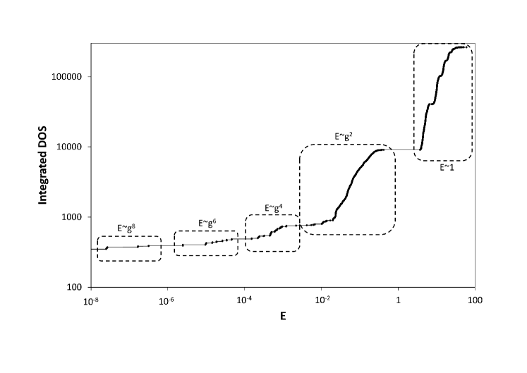
Figure 3: Integrated density of states of model $(a)$ for $N=18$ and $\Delta_{1}=5$.

The distribution of the energy levels for $N=18$ and $g=0.1$ for the model $(a)$ is shown in Fig.3 (model $(b)$ has a very similar picture of energy levels). As it can be seen in Fig.3 the spectrum is distinctly divided into some parts. Each part of the spectrum behaves as $E\sim g^{2k}$ as depicted in Fig.3. This fact was confirmed numerically by the comparison of the energies for $g=0.1$ and $g=0.125$.

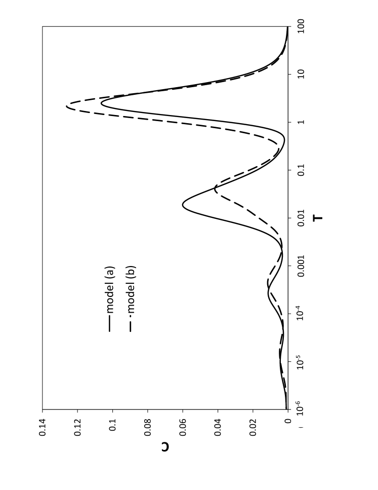
Figure 4: Dependence of the specific heat on the temperature for $N=18$ and $\Delta_{1}=5$.

Such structure of the spectrum determines the characteristic features of the low-temperature thermodynamics. To study the thermodynamics of model (29) we use the exact diagonalization of finite kagome chains with PBC up to $N=18$. In Fig.4 we represent the data for the specific heat $C(T)$ (per site) for $\Delta_{1}=5$ ($g=0.1$) obtained by the ED for $N=18$. The temperature dependence of the specific heat shown in Fig.4 exhibits numerous maxima for both models $(a)$ and $(b)$. The peak at $T\geq 1$ is formed by the states with $E\geq 1$ and the low-temperature maxima are related to the corresponding parts of the spectrum with the energies $E\sim g^{4}$, $E\sim g^{6}$ and so on.

Figure 5: Dependence of the specific heat on the temperature for model $(a)$ at $\Delta_{1}=5$ and for $N=15,18$.

To estimate the finite-size effects we compare the data of $C(T)$ for $\Delta_{1}=5$ for $N=15$ and $N=18$ (model a). As it can be seen in Fig.5 the data of $C(T)$ for $N=15$ and $N=18$ deviate from each other for $T\lesssim 10^{-4}$ but they are very close for $T\gtrsim 10^{-4}$. This indicates that the obtained finite-size data correctly describe the thermodynamic limit for temperatures $T\gtrsim 10^{-4}$. (We note that a similar conclusion is valid for other values of the anisotropy). The deviation of the data for $N=15$ and $N=18$ in the region $T\lesssim 10^{-4}$ means that the finite-size effects become essential for $T\lesssim 10^{-4}$ and that the correct description of the thermodynamics in this temperature region requires the consideration of larger systems. Nevertheless, the multi-scale structure of the spectrum for $\Delta_{1}\gg 1$ will lead certainly to the existence of many maxima in $C(T)$ and their number is proportional to the system size.

Figure 6: Dependence of the specific heat on the temperature for $N=18$ and $\Delta_{1}=2$.

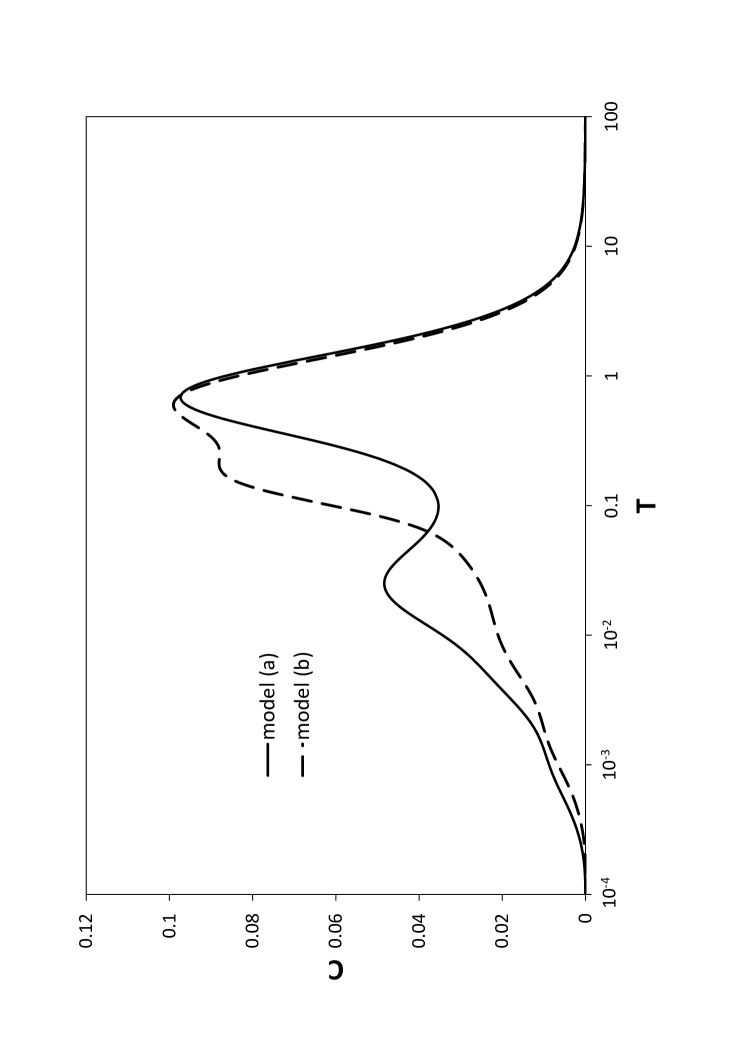
Figure 7: Dependence of the specific heat on the temperature for $N=18$ and $\Delta_{1}=1$.

With decreasing of $\Delta_{1}$ the many-peak dependence of $C(T)$ becomes less pronounced and vanishes for $\Delta_{1}<3$. For $\Delta_{1}<3$ the only one low-temperature maximum in $C(T)$ curve survives for model $(a)$. For model $(b)$ the low-temperature maximum transforms into shoulder as shown in Figs.6, 7.

IV Isotropic models

As we noted before the ground state degeneracy is the same throughout the whole transition line including the isotropic point $\Delta_{1}=\Delta_{2}=1$. As to the energy gaps for the excited states they show a sharp decrease with an increase of the number of magnons, $k$, similarly to the case of large anisotropy $\Delta_{1}\gg 1$. However, the behavior of the gap $E(k,n)$ in the isotropic model is rather specific. The analysis of the numerical calculations of finite kagome-chains shows that the behavior of the gap $E(k,n)$ is qualitatively different in the sectors $k<\frac{n}{2}$ and $k>\frac{n}{2}$. For relatively small number of magnons, $k<\frac{n}{2}$, the gap rapidly decreases with the increase of $k$, so that for long chains ($n\gg 1$) it can be approximated as $E(k,n)\sim\exp(-2\gamma k)$ with $\gamma\simeq 2.80$. This value of the gap represents the energy of $k$-magnon bound complex. On the boundary between these two sectors, i.e. for $k=\frac{n}{2}$, the gap is $E_{b}\sim\exp(-\gamma n)$. When the number of magnons exceeds the value $\frac{n}{2}$, the gap ceases to decrease rapidly and only slightly changes with $k$ and $n$, so that the gap approximately holds its boundary value $E(k,n)\sim\exp(-\gamma n)$. Thus, the studied system has a quite unusual property of exponentially small gaps, and this fact is attributed to the smallness of the energy of the multi-magnon bound complexes.

at fixed number of magnons $k<\frac{n}{2}$ the gap behaves as Now let us examine the type of the phase transition which occurs on the studied isotropic transition point. At $J_{a}<\frac{1}{2}$ or $J_{b}<\frac{1}{4}$ the ground state is ferromagnetic. In the transition points $J_{a}=\frac{1}{2}$ and $J_{b}=\frac{1}{4}$ the spontaneous magnetization is $\frac{M}{N}=\frac{1}{3}$ according to Eq.(20) (such ground state magnetization is on the entire transition line). It is interesting to find out what is the ground state magnetization for $J_{a}>\frac{1}{2}$ or $J_{b}>\frac{1}{4}$, especially in the vicinity of the transition points. For this aim we have employed numerical calculations with the use of both the ED method and the density matrix renormalization group (DMRG) algorithm. The ED is used for the consideration of the finite kagome chains up to $N=24$ spins. The DMRG method allows to explore much larger chains. In our calculations we considered the chains up to $N=240$ spins. Our results show that the magnetization is $\frac{M}{N}=\frac{1}{3}$ in the close vicinity of the transition points, at least up to deviation $0.05$ from the transition points. Local magnetizations in this ferrimagnetic state are $\langle\sigma_{i}^{z}\rangle=\langle\xi_{i}^{z}\rangle\simeq 0.3$, $\langle S_{i}^{z}\rangle\simeq 0.4$. The spontaneous magnetization decreases with the increase of $J_{a,b}$ and tends to $\frac{M}{N}=\frac{1}{6}$ at $J_{a,b}\gg 1$. The question about the behavior of the magnetization in the region of the intermediate values of $J_{a,b}$ requires further studies.

The main conclusion of our present examination is that the magnetization has a jump in the transition points from $\frac{M}{N}=\frac{1}{2}$ on the ferromagnetic side of the ground state phase diagram to $\frac{M}{N}=\frac{1}{3}$ in the ferrimagnetic region, justifying the first-order type of the phase transition.

V Summary

We have studied the ground state and the low-temperature properties of two models of the kagome-like chains with the anisotropic ferromagnetic and the antiferromagnetic exchange interactions. We focus on the model behavior on the transition line between the ferromagnetic and the ferrimagnetic ground state phases. This transition line is parameterized by the anisotropy of the leg-axis interaction $\Delta_{1}$ which varies from $\Delta_{1}=1$ (the isotropic case) to $\Delta_{1}\to\infty$ (the Ising model). On this line the ground state manifold consists of both the localized multimagnon states and the special multimagnon complexes. The ground state degeneracy is macroscopic and there is the residual entropy at $T=0$. In the limiting case $\Delta_{1}=\infty$ the considered models reduce to Ising kagome-chains. The ground state degeneracy of these Ising models is huge though it is different for the kagome chains $(a)$ and $(b)$. For finite anisotropy $\Delta_{1}$ this degeneracy is partially lifted. Remarkably, firstly the ground state degeneracy is the same throughout the whole transition line and secondly it is the same (with minor difference) for both models in spite of different degeneracy of corresponding limiting Ising kagome-chains.

We found that the kagome chains on the transition line have finite spontaneous magnetization, while the ground state of these models in the Ising limit is magnetically disordered (zero magnetization). It means that the quantum effects induced by the perturbations $V_{1}$ and $V_{2}$ (Eqs.(30)) in the classical (Ising) model with disordered degenerate ground state lead to magnetically ordered state, so demonstrating the ‘order by disorder’ phenomenon.

The characteristic feature of the considered models is the jump of the spontaneous magnetization in the transition point of the ground state phase diagram of the isotropic models. Our examination shows that similar jump takes place on the entire transition line too.

For $\Delta_{1}\gg 1$ the excitation spectrum has multi-scale structure and is rank-ordered in powers of small parameter $\Delta_{1}^{-2}$. The number of sections of the spectrum is equal to the chain length $n$ and the energy of the levels in the $m$-th section is $E\sim\Delta_{1}^{-2m+2}$ ($m=1,\ldots n$). The origin of such exponentially low energy levels is the fact that the $m$-magnon bound complex in this system has the energy $E_{m}\sim\Delta_{1}^{-2m+2}$. Each $m$-th section of the spectrum is responsible for the appearance of $m$-th peak in the specific heat curve $C(T)$. Thus, the number of the peaks in the specific heat grows with the length of the chain. Numerical calculations by the ED of finite chains show that such behavior of $C(T)$ is qualitatively similar for $\Delta_{1}>3$ but it is modified in a definite way for $\Delta_{1}<3$. In particular, the specific heat has one low-temperature maximum in model $(a)$ and the shoulder in $C(T)$ dependence for model $(b)$.

The kagome-chain $(b)$ is related to the copper-oxide compounds $\mathrm{Ba_{3}Cu_{3}In_{4}O_{12}}$ and $\mathrm{Ba_{3}Cu_{3}Sc_{4}O_{12}}$. Though in this model the interchain interaction leading to the low-temperature phase transition is not taken into account it can be considered as the minimal model for the description of the paramagnetic phase of these systems. In these compounds the antiferromagnetic leg-leg exchange interaction $J_{b}$ is small and in the first approximation can be neglected so that the model becomes pure ferromagnetic one. Such ferromagnetic model has been studied in Refs.soos1 ; soos and it gives rather adequate description of the paramagnetic phase of real compounds. Though in the kagome chain considered by us the AF interaction $J_{b}$ is not small and corresponds to special model parameter we believe that this model as well as the model $(a)$ show rather unusual properties which can be observed in compounds of similar geometrical structure.

In this paper we have studied two version of the kagome chains corresponding to special choice of the antiferromagnetic leg-leg exchange interactions: $J_{2}\neq 0$, $J_{3}=0$ and $J_{2}=J_{3}$. However, our consideration can be easily extended to the more general case $J_{2}\neq J_{3}$.

The numerical calculations were carried out with use of the ALPS libraries alps .

References

- (1) H. T. Diep, ed., Frustrated spin systems (World Scientific, Singapore, 2013).
- (2) C. Lacroix, P. Mendels and F. Mila, eds., Intoduction to frustrated magnetism. Materials, Experiments, Theory (Springer-Verlag, Berlin, 2011).
- (3) O. Derzhko, J. Richter, M. Maksymenko, Int. J. Modern Phys. 29, 1530007 (2015).
- (4) J. Richter, O. Derzhko and J. Schulenburg, Phys.Rev.Lett. 93, 107206 (2004).
- (5) M. Maksymenko, A. Honecker, R. Moessner, J. Richter, and O. Derzhko, Phys. Rev. Lett. 109, 096404 (2012).
- (6) M.E. Zhitomirsky and H. Tsunetsugu, Progr. Theor. Phys. Suppl. 160, 361 (2005).
- (7) J. Schnack, H.-J. Schmidt, J. Richter and J. Schulenberg, Eur. Phys. J. B 24, 475 (2001).
- (8) J. Richter, J. Schulenburg, A. Honecker, J. Schnack, and H.J. Schmidt, J. Phys.: Condens. Matter 16, S779 (2004).
- (9) M.E. Zhitomirsky and H. Tsunetsugu, Progr. Theor. Phys. Suppl. 160, 361 (2005).
- (10) O. Derzhko and J. Richter, Phys. Rev. B 70, 104415 (2004).
- (11) V. Ya. Krivnov, D. V. Dmitriev, S. Nishimoto S.-L. Drechsler, and J. Richter, Phys. Rev. B 90, 014441 (2014).
- (12) D. V. Dmitriev and V. Ya. Krivnov, Phys.Rev. B 92, 184422 (2015).
- (13) Ch. Waldtman, H. Kreutzmann, U. Schollwock, K. Maisinger and H. -U. Everts, Phys. Rev. B 62, 9472 (2000).
- (14) E. Lieb and D. Mattis, J. Math. Phys. 3, 749 (1962).
- (15) J. Schulenburg, A. Honecker, J. Schnack, J. Richter and H. -J. Schmidt, Phys. Rev. Lett. 88, 167207 (2002).
- (16) O. S. Volkova, I. S. Maslova, R. Klingigiler, M. Abdrl-Hafiez, Y. C. Araugo, A. U. B. Wolter, V. Kataev, B. Buchner and A. N. Vasiliev, Phys. Rev. B 85, 104420 (2012).
- (17) S. E. Dutton, M. Kumar, Z. G. Soos, C. L. Broholm and R. J. Cava, J. Phys.: Condens. Mat., 24, 166001 (2012).
- (18) M. Kumar, S. E. Dutton, R. J. Cava and Z. G. Soos, J. Phys.: Condens. Mat. 25, 136004 (2013).
- (19) D. I. Bartdinov, O. S. Volkova, A. A. Tsirlin, I. V. Solovyev, A. N. Vasiliev and V. V. Mazurenko, Phys. Rev. B 94, 054435 (2016).
- (20) B. Koteswararao, A. V. Mahajan, F. Bert, P. Mendels, J. Chakraborty, V. Singh, I. Dasgupta, S. Rayaprol, V. Siruguri, A. Hoser and S. D. Kaushik, J.Phys.:Condens.Mat. 24, 236001 (2012).
- (21) B. Bauer et al., J. Stat. Mech. P05001 (2011).