Deconstructing temperature gradients across fluid interfaces: the structural origin of the thermal resistance of liquid-vapor interfaces

Abstract

The interfacial thermal resistance determines condensation-evaporation processes and thermal transport across material-fluid interfaces. Despite its importance in transport processes, the interfacial structure responsible for the thermal resistance is still unknown. By combining non-equilibrium molecular dynamics simulations and interfacial analyses that remove the interfacial thermal fluctuations we show that the thermal resistance of liquid-vapor interfaces is connected to a low density fluid layer that is adsorbed at the liquid surface. This thermal resistance layer (TRL) defines the boundary where the thermal transport mechanism changes from that of gases (ballistic) to that characteristic of dense liquids, dominated by frequent particle collisions involving very short mean free paths. We show that the thermal conductance is proportional to the number of atoms adsorbed in the TRL, and hence we explain the structural origin of the thermal resistance in liquid-vapor interfaces.

The interfacial thermal resistance describes the abrupt change of temperature, $\Delta T$, at the surface between two distinct bulk phases, when a heat flux $J_{q}$ goes across it. The effect was originally postulated for liquid helium/solid interfaces, as a consequence of the sharp change in the nature of the heat carriers, and it was first measured by Kapitza in 1941 Kapitza (1941); Swartz and Pohl (1989) in terms of what is known as the Kapitza resistance $R_{K}=\Delta T/J_{q}$, or the interfacial conductance $G_{K}=1/R_{K}$. In a bulk phase, the thermal conductivity $\lambda$ gives the ratio between the temperature gradient and the heat current, so that the different bulk conductivities produce different slopes in the temperature profile $T(z)$ at the two sides of the interface. At the interface, the temperature profile features a sharp ‘jump’, $\Delta T=J_{q}/G_{K}$, reflecting the physical mechanism associated to energy transfer between heat carriers in the different phases in contact. Hence, $R_{K}$ or $G_{K}$ provide insight into the molecular structure of the interface and the microscopic mechanism determining energy transport.

Since the seminal work by Kapitza, the concept of interfacial thermal resistance has been extended to describe energy flux across many other interfaces and to identify the relevant transport channels for heat transfer. Understanding the physical origin of the thermal resistance would provide fundamental information on the coupling between the heat carriers at the two sides of an interface. This problem is of significant interest in many current technologies, e.g. in microelectronics, the management of energy transport in the form of heat is of utmost importance. Further, with the advent of ever more advanced experimental techniques, the increasing spatial and temporal resolution to characterize thermal transport is approaching the atomistic length scales characteristic of nanometric devices Cui et al. (2017); Capinski et al. (1999).

Thermal conduction across fluid-fluid interfaces sets also important fundamental and applied challenges for the study of condensation-evaporation processes Caputa and Struchtrup (2011), thermal resistance of nanomaterials Luo and Chen (2013); Wilson et al. (2002); Cahill et al. (2014); Tascini et al. (2017) and biological interfaces Leitner and Straub (2010); Yu and Leitner (2005); Lervik et al. (2010). The thermal resistance can be quite significant when the phases in contact involve appreciable differences in density, e.g., in a liquid-vapor interface away from the critical region the large density difference between the liquid ($l$) and the ($g$) phases ($\rho_{l}/\rho_{g}\sim 10^{2}-10^{3}$) involves a qualitative change in the mechanism of heat transport. In liquids the mechanism is dominated by molecular collisions of atoms/molecules inside the cage formed by the nearest neighbors, without the need of mass diffusion. In low density gases the thermal transport involves long ballistic flights and long mean free paths, e.g. ten to hundred molecular diameters near triple point conditions. Under a given heat flow, the bulk thermal conductivities are very different, $\lambda_{l}\gg\lambda_{g}$ resulting in important changes in the slope of the temperature profile across the interface Røsjorde et al. (2000); Simon et al. (2004); Jackson, Rubi, and Bresme (2016). Theoretical studies demonstrate that kinetic theory offers an accurate approach to quantify the thermal conductance of simple fluids and good agreement with simulations has been reported Kjelstrup and Bedeaux (2008a).

At the sharpest molecular scale employed in computer simulations, the temperature profile $T(z)$ may be consistently obtained either from the mean kinetic energy or the forces Jackson, Rubi, and Bresme (2016) on atoms or molecules located at position $z$. The slope of $T(z)$ at the vapor and liquid phases is determined by the thermal conductivity of each phase, $\lambda_{g}$ and $\lambda_{l}$. Kapitza’s mesoscopic view considers the approximate description of $T(z)$ as straight lines with slopes $J_{q}/\lambda_{g}$ and $J_{q}/\lambda_{l}$, with a temperature ‘jump’ $\Delta T=J_{q}/G_{K}$ at position $z_{K}$ (see Supporting Information). Intriguingly, previous theoretical studies indicate that $z_{K}$ is shifted towards the vapor phase. The molecular interpretation of $z_{K}$ and $G_{K}$ has been elusive because fluid interfaces, liquid/vapor or liquid/liquid, feature capillary waves that blur out the molecular structure of the interface Rowlinson and Widom (2003). This results in a broadening of the density ($\rho(z)$) and temperature ($T(z)$) profiles, which eliminates important structural details of the interface. Our hypothesis is that by removing the thermal fluctuations we can resolve the interfacial structure and hence identify the key regions defining the interfacial thermal resistance. To illustrate our idea, we study the liquid-vapor interface of a simple fluid.

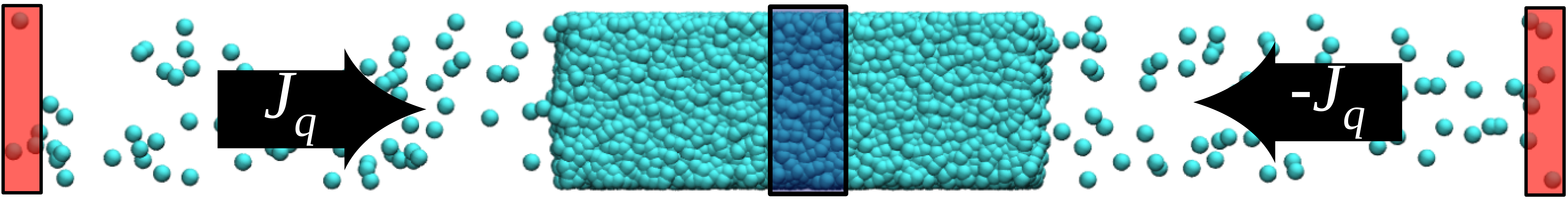
Figure 1: Schematic diagram showing the periodic simulation cell containing a liquid-vapor interface. The liquid phase is in the center of the box. The spheres represent the atoms. Kinetic energy is extracted in the centre of the liquid phase (blue highlighted region) and added in the center of the gas phase (red highlighted regions) at a constant rate. The arrows indicate the direction of the resultant energy flux. It should be noted that the actual simulation cells used in the simulations are significantly more elongated in the $z$-direction than in this snapshot.

Stillinger introduced the concept of intrinsic surface (IS), a time dependent surface that can be used to describe the interfacial structure by removing capillary wave effects Stillinger (1982). The intrinsic sampling method (ISM) Chacón and Tarazona (2003) allows to identify the IS, making it possible to resolve the molecular structure of the interface Chacón and Tarazona (2003); Bresme, Chacón, and Tarazona (2008). In this work we apply the ISM to a liquid-vapor interface under an applied heat flux. By doing so we are able to identify the structural origin of the thermal resistance.

The simulations were performed on a system of Lennard-Jones particles at varying temperatures along the coexistence line. Reduced units are used for all the quantities throughout the paper, unless otherwise indicated. The heat flux was induced by creating a region of energy extraction (cold region) in the centre of the liquid slab and by adding energy at the edges of the simulation box, in the vapor phase (hot region) (see Figure 1). The heat flux is given by,

$$J_{q}=\frac{\pm\dot{Q}}{2L_{x}L_{y}}$$ (1)

Where $\dot{Q}$ is the rate of kinetic energy added(+)/withdrawn(-) from the hot/cold regions, and $L_{x}L_{y}$ is the cross sectional area of the simulation box (see Supplementary Information and references LAM ; Hafskjold, Ikeshoji, and Ratkje (1993)). We used $\dot{Q}=5$ or $10$ for system I and II, III, respectively (see Figure 2). For system I and II the heat flux corresponds to $3.3\times 10^{7}\text{ Wm}^{-2}$ in SI units.

Our simulations reach a stationary state with no net mass flux, which allows the decoupling of heat and mass transfer processes and hence the computation of the thermal resistance from the temperature profiles (see ref. Kjelstrup and Bedeaux (2008b) for a discussion of coupled processes). Lack of thermalization may appear in the Knudsen layer in systems featuring strong evaporation. This effect is not relevant in our case, due to the lack of mass flux. This is supported by the similarity of temperature profiles obtained for systems featuring very different vapor densities, and by earlier work that showed the consistency of the local temperatures computed using kinetic and configurational approaches Jackson, Rubi, and Bresme (2016).

In the capillary wave theory formalism the intrinsic surface is defined as

$$z=\xi(\mathbf{R},q_{u})\;,\;\mathbf{R}=(x,y)$$ (2)

where the wavevector cutoff, $q_{u}$, determines the level of resolution of the surface. The intrinsic surface can be expressed in terms of a Fourier series,

$$\xi(\mathbf{R},q_{u})=\hat{\xi}_{0}+\sum_{0<|\mathbf{q}|<q_{u}}\hat{\xi}_{q}e^{i\mathbf{q}\cdot\mathbf{R}}.$$ (3)

The ISM identifies the intrinsic surface via a percolation method, and uses an iterative procedure to calculate the Fourier coefficients associated with each wavevector in the expansion of the intrinsic surface. This is performed for various occupancy values, $n_{S}=N_{S}/A_{0}$, where $N_{S}$ is the number of atoms at the intrinsic surface and $A_{0}$ is the cross sectional area of the interface. We chose in this work $n_{s}=1.0$ for systems I and II and $n_{s}=0.7$ for system III. We find that these parameters provide a good resolution of the interfacial structure (see the SI for other occupancies). The intrinsic density and temperature profiles were computed with respect to the intrinsic surface $\xi(\mathbf{R})$ defined above.

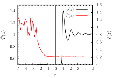
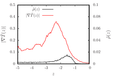
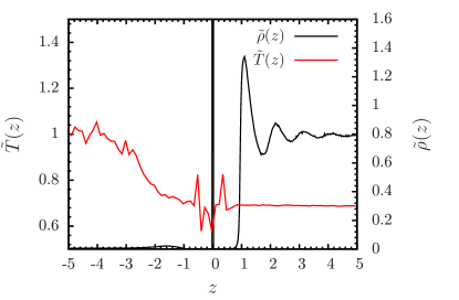
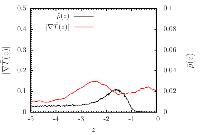
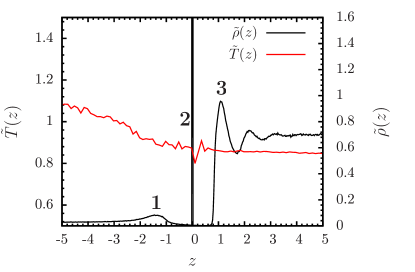
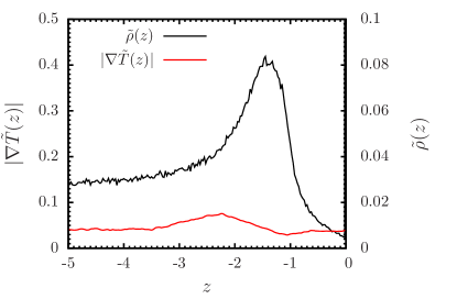
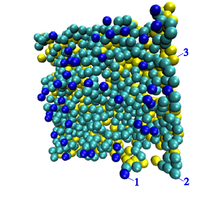
Figure 2: Top-Left panels: Intrinsic temperature profiles ($\tilde{T}(z)$, red line) and intrinsic density profiles ($\tilde{\rho}(z)$, black line) for systems at different average temperatures, system I (top), system II (middle), and system III (bottom). Top-Right panels: Absolute values of the gradient of the intrinsic temperature profiles ($|\nabla\tilde{T}(z)|$, red line) and intrinsic density profiles ($\tilde{\rho}(z)$, black line) shifted and scaled to highlight the adsorbed layer for systems I (top), II (middle) , and III (Bottom). The numerical derivative of the temperature profile is calculated from data averaged over a 0.2$\sigma$ window with the derivative further smoothed over a window of the same size. The labels ‘1, 2, 3’ refer to the fluid layers represented in the bottom panel. Bottom-central panel: Representative surface configuration for system III. Atoms at the IS are represented in cyan. The atoms colored in blue represent the first layer in the vapor phase, and the yellow atoms the first liquid layer.

The intrinsic profiles for different liquid temperatures are shown in Figure 2. The delta function peaks in the density profiles (located at $z=0.0$) are defined by the $N_{s}$ surface atoms at the IS. The oscillations in the liquid phase reflect the ordered layers of atoms in the liquid with respect to the IS. It can also be seen that there is a low density peak in the vapor region. While small as compared to the bulk liquid density, the peak is large in comparison to the bulk density of the vapor (see right panels in Figure 2). This peak is connected to the adsorption of atoms at the intrinsic surface. In the percolation analysis performed in the ISM, these atoms are identified as protrusions in the percolating cluster that defines the liquid surface and are connected to the bulk liquid, typically, by less than three neighbors. A visual representation of the configuration of particles corresponding to the peaks either side of the intrinsic surface ($z=0.0$) illustrates this idea (see Figure 2). Particles colored in cyan represent the atoms belonging to the $N_{S}$ surface sites in the IS. The particles colored in yellow represent the atoms in the interval $0.7\leq z<1.7$, i.e. the first liquid layer. The particles colored in blue (interval $-2.7\leq z<0.0$) correspond to atoms in the layer adsorbed at the IS. Effectively, the adsorption layer is similar to that formed by a gas adsorbing on a rough solid substrate.

The thermal boundary resistance is located in the vapor phase, above the liquid surface (see $\tilde{T}(z)$ and $|\nabla\tilde{T}(z)|$ in Figure 2). The temperature of the liquid surface (see Figure 2), is essentially the same as that of the bulk liquid. The thermal resistance, as given by the temperature drop from the vapor to the liquid phase, depends strongly on the average temperature of the run, and as expected, it is more prominent at low temperatures, indicating higher resistance to thermal transport. At higher temperatures the difference in temperature between the two bulk phases decreases significantly, as exemplified by case III in Figure 2.

At the molecular scale, the thermal resistance does not lead to a discontinuity in the temperature profile, but instead to a larger but continuous variation of the temperature gradient over a small length scale of a few atomic radii. This drop in temperature appears immediately above the liquid surface. Figure 2 shows the absolute value of the thermal gradient with reference to the intrinsic density profile in the vapor phase. The region of maximum thermal resistance coincides with the adsorption peak in the density of the vapor phase. As the density of the adsorbed layer decreases, the temperature gradient, and therefore the thermal resistance, increases. We propose that the adsorbed layer, the thermal resistance layer (TRL), controls the exchange of heat between the liquid and vapor phases.

Interface	System	$L_{x}$/$\sigma$	$L_{z}$	$\dot{Q}$	$\lambda_{V}$	$\lambda_{L}$	$G_{K}$
Liquid/Vapour	I	22.2	1368.0	5	0.65	6.53	0.011
Liquid/Vapour	II	22.2	1368.0	5	0.72	6.00	0.020
Liquid/Vapour	III	20.5	256.5	10	0.55	5.00	0.082

Table 1: Summary of thermal transport properties calculated for all systems simulated in this work, including the thermal conductivities in the vapor phase ($\lambda_{V}$) and liquid phase ($\lambda_{L}$) and the interfacial thermal conductance ($G_{K}=J_{q}/\Delta T$). The rate of energy input ($\dot{Q}$) is also listed along with the system dimensions and initial temperature before a heat flux is applied. All quantities are in reduced units.

In order to calculate the thermal conductance, $G_{K}$, an extrapolation of $\tilde{T}(z)$ from each bulk phase is taken up to a precise ‘thermal boundary’ located at $z_{K}$, at which the temperature ‘jump’, $\Delta T$, can be calculated. This temperature ‘jump’ provides a nanoscopic description of thermal transport at the interface. The obvious choice to define $z_{K}$ is given by the integral of the local temperature deviation with respect to the temperature in the bulk gas, $T_{g}(z)$, and liquid, $T_{l}(z)$, phases,

$$\int_{z_{g}}^{z_{K}}(\tilde{T}(z)-T_{g}(z))dz+\int_{z_{K}}^{z_{l}}(\tilde{T}(z)-T_{l}(z))dz=0,$$ (4)

where the positions $z_{g}$ and $z_{l}$ are located well within the respective asymptotic regimes $\tilde{T}(z)=T_{g}(z)$ for $z<z_{g}$ and $\tilde{T}(z)=T_{l}(z)$ for $z>z_{l}$. An illustration of how we identify $z_{K}$ is given in the SI. The approach introduced here provides a unique definition of the temperature ‘jump’, as there is no need to define an arbitrary location for the extrapolation of the temperature profiles in order to calculate $\Delta T$.

The values of the interfacial thermal resistance for each average temperature are reported in Table 1 along with the thermal conductivities of the respective bulk phases. The thermal conductance increases with increasing average temperature, changing in magnitude by a factor of eight from system I to system III. This increase is accompanied by an enhancement of the thermal conductivity and density in the gas phase. The thermal conductivities in the liquid phase are of the same order as the experimental values for argon Linstrom and Mallard (2006). The simulated thermal conductivity for system II (temperature of the liquid $\sim$84 K) is $\lambda_{L}=0.11\text{ Wm}^{-1}\text{K}^{-1}$, in good agreement with experimental data, $\lambda_{L}=0.13\text{ Wm}^{-1}\text{K}^{-1}$.

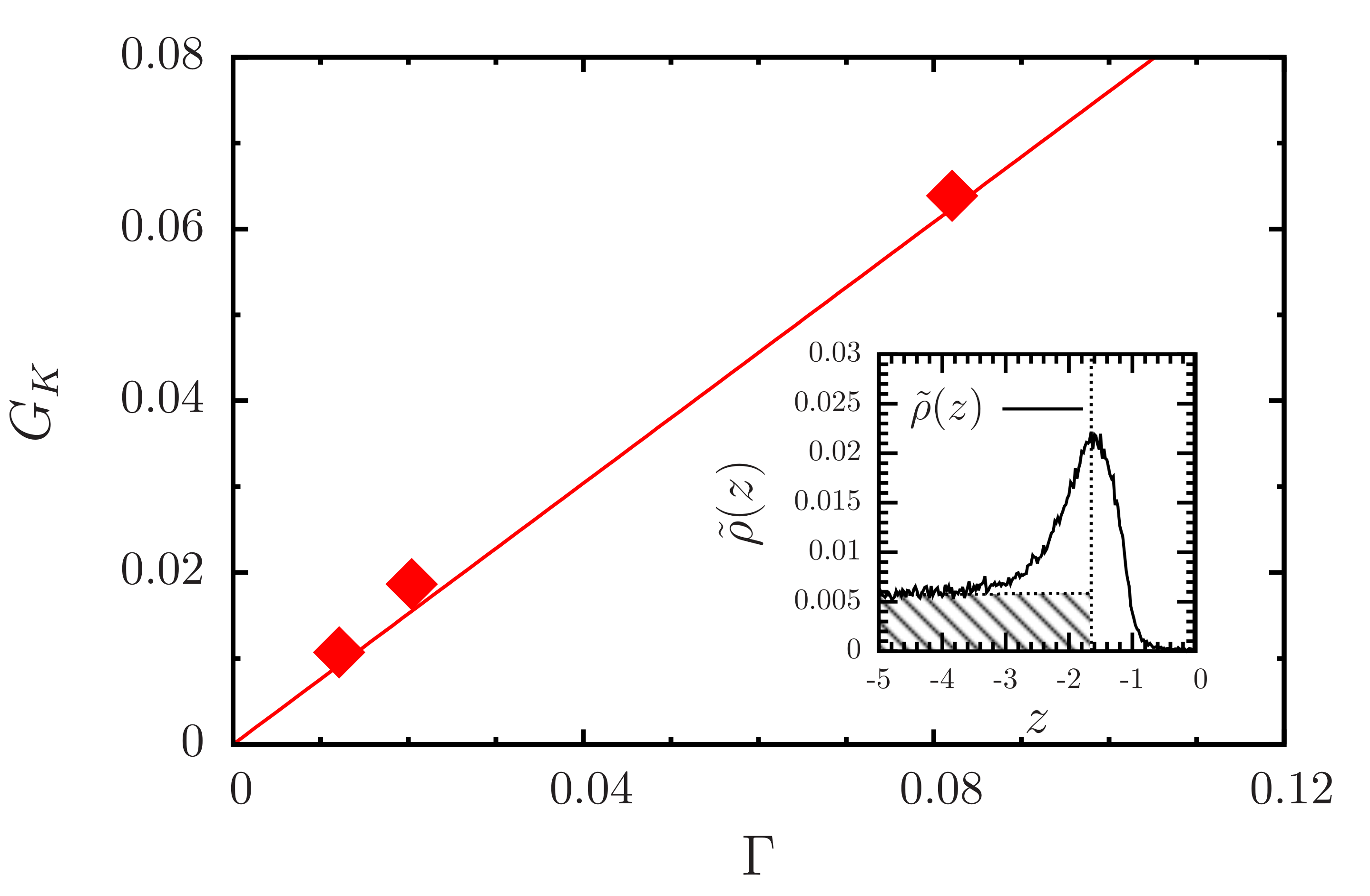
Figure 3: Thermal conductance $G_{K}$ against adsorption $\Gamma$. The red line is a guide for the eye. The inset plot illustrates the calculation of the adsorption from equation (5) for system II. The shaded region is subtracted from the integral over the intrinsic density profile.

We compute now the fluid adsorption associated to the TRL. We define the adsorption as

$$\Gamma=\frac{1}{m}\int_{-\infty}^{0}\tilde{\rho}(z)dz-\frac{1}{m}\int_{-\infty}^{z_{\text{max}}}\rho_{g}(z)dz$$ (5)

where $m$ is the mass of the particle ($m=1$ in reduced units), $\rho_{g}(z)$ is a linear extrapolation of the density profile in the vapor phase at sufficient distance from the interface and $z_{\text{max}}$ is the position of the local maximum due to adsorbed particles. Figure 3 shows the thermal conductance $G_{K}$ plot as a function of the surface adsorption $\Gamma$ for the systems I, II, and III discussed above. A linear relationship is observed between the conductance and the adsorption, supporting the notion that the thermal resistance is governed by the degree of adsorption in the TRL that separates the liquid surface from the vapor phase.

We have shown that the combination of non-equilibrium molecular dynamics simulations and intrinsic sampling approaches provides a route to identify the interfacial structure defining the thermal resistance of liquid-vapor interfaces. We draw the following conclusions from our study:

$\bullet$ The thermal conductance of liquid-vapour interfaces is defined by the thermal resistance layer, which is located at $\sim 2$ molecular diameters from the mean position of the liquid surface and shifted towards the vapor phase. The TRL is a boundary resistance layer for the transition from ballistic thermal transport (vapor), to thermal transport dominated by atomic/molecular collisions inside the cage formed by the nearest neighbors (liquid).

$\bullet$ The liquid surface (defined by the intrinsic surface) and the bulk liquid have essentially the same temperature.

$\bullet$ In the sharpest representation of the interface, obtained with the ISM, the TRL is defined by a local maximum in the density in the vapor region. The TRL is defined by the adsorption of a low density monolayer at the liquid surface, which within the ISM percolation analysis correspond to atom ‘overhangs’ of the liquid phase. The transition in the heat transfer mechanism between the vapor and the liquid phases, proceeds via the atomic overhangs, which form via a dynamical equilibrium where molecules from the hot gas get trapped after a collision with the liquid surface and molecules from the cold liquid reach the surface and eventually detach from it. The sharp temperature change $\Delta T$ at the TRL reflects precisely the energy transfer between these two distinct types of heat carriers.

$\bullet$ The density of the TRL increases as the critical point is approached, i.e. with the density of the coexisting vapor. The thermal conductance increases linearly with the number of particles in the TRL.

We propose that the TRL is the key molecular structure determining the thermal transport across liquid-vapor interfaces and that the number of heat carriers in the TRL may be quantified in computer simulations when the blurring effects of the capillary waves are eliminated from the temperature profile $T(z)$. Further work will focus on the investigation of the thermal resistance of multicomponent systems.

We acknowledge the EPSRC-UK (EP/J003859/1) and the Spanish Secretariat for Research, Development and Innovation (Grant No. FIS2013-47350-C5 and MDM-2014-0377) for financial support. We thank the Imperial College High Performance Computing Service for providing computational resources and Dick Bedeaux for insightful discussions on heat transport across interfaces.

References

- Kapitza (1941) P. L. Kapitza, Phys. Rev. 60, 354–355 (1941).
- Swartz and Pohl (1989) E. T. Swartz and R. O. Pohl, Rev. Mod. Phys. 61, 605–668 (1989).
- Cui et al. (2017) L. Cui, W. Jeong, S. Hur, M. Matt, J. C. Klöckner, F. Pauly, P. Nielaba, J. C. Cuevas, E. Meyhofer, and P. Reddy, Science 355, 1192–1195 (2017).
- Capinski et al. (1999) W. S. Capinski, H. J. Maris, T. Ruf, M. Cardona, K. Ploog, and D. S. Katzer, Phys. Rev. B 59, 8105–8113 (1999).
- Caputa and Struchtrup (2011) J. P. Caputa and H. Struchtrup, Physica A 390, 31–42 (2011).
- Luo and Chen (2013) T. Luo and G. Chen, Phys. Chem. Chem. Phys. 15, 3389–3412 (2013).
- Wilson et al. (2002) O. M. Wilson, X. Hu, D. G. Cahill, and P. V. Braun, Phys. Rev. B 66, 224301 (2002).
- Cahill et al. (2014) D. G. Cahill, P. V. Braun, G. Chen, D. R. Clarke, S. Fan, K. E. Goodson, P. Keblinski, W. P. King, G. D. Mahan, A. Majumdar, H. J. Maris, S. R. Phillpot, E. Pop, and L. Shi, Appl. Phys. Rev. 1, 011305 (2014).
- Tascini et al. (2017) A. S. Tascini, J. Armstrong, E. Chiavazzo, M. Fasano, P. Asinari, and F. Bresme, Phys. Chem. Chem. Phys. 19, 3244–3253 (2017).
- Leitner and Straub (2010) D. M. Leitner and J. E. Straub, Proteins, Energy, Heat and Signal Flow, 1st ed. (CRC Press, 2010).
- Yu and Leitner (2005) X. Yu and D. Leitner, J. Chem. Phys. 122 (2005).
- Lervik et al. (2010) A. Lervik, F. Bresme, S. Kjelstrup, D. Bedeaux, and J. M. Rubi, Phys. Chem. Chem. Phys. 12, 1610–1617 (2010).
- Røsjorde et al. (2000) A. Røsjorde, D. Fossmo, D. Bedeaux, S. Kjelstrup, and B. Hafskjold, J. Colloid Interface Sci. 232, 178–185 (2000).
- Simon et al. (2004) J. Simon, S. Kjelstrup, D. Bedeaux, and B. Hafskjold, J. Phys. Chem. B 108, 7186–7195 (2004).
- Jackson, Rubi, and Bresme (2016) N. Jackson, J. Rubi, and F. Bresme, Mol. Sim. 42, 1214–1222 (2016).
- Kjelstrup and Bedeaux (2008a) S. Kjelstrup and D. Bedeaux, Non-Equilibrium Thermodynamics of Heterogeneous Systems (World Scientific, 2008).
- Rowlinson and Widom (2003) J. S. Rowlinson and B. Widom, Molecular Theory of Capillarity (Dover Publications Inc., 2003).
- Stillinger (1982) F. H. Stillinger, J. Chem. Phys. 76, 1087 (1982).
- Chacón and Tarazona (2003) E. Chacón and P. Tarazona, Phys. Rev. Lett. 91 (2003).
- Bresme, Chacón, and Tarazona (2008) F. Bresme, E. Chacón, and P. Tarazona, Phys. Chem. Chem. Phys. 10, 4704–4715 (2008).
- (21) LAMMPS Users Manual, Sandia National Laboratories.
- Hafskjold, Ikeshoji, and Ratkje (1993) B. Hafskjold, T. Ikeshoji, and S. K. Ratkje, “On the molecular mechanism of thermal-diffusion in liquids,” Mol. Phys. 80, 1389–1412 (1993).
- Kjelstrup and Bedeaux (2008b) S. Kjelstrup and D. Bedeaux, Non-Equilibrium Thermodynamics of Heterogeneous Systems, 1st ed. (World Scientific, 2008).
- Linstrom and Mallard (2006) P. Linstrom and W. Mallard, eds., Thermophysical Properties of Fluid Systems, National Institute of Standards and Technology, Gaithersburg MD, 20899, http://webbook.nist.gov, (retrieved May 29, 2011) (2006).