Atomic-Scale Magnetometry of Dynamic Magnetization

Abstract

The spatial resolution of imaging magnetometers has benefited from scanning probe techniques. The requirement that the sample perturbs the scanning probe through a magnetic field external to its volume limits magnetometry to samples with pre-existing magnetization. We propose a magnetometer in which the perturbation is reversed: the probe’s magnetic field generates a response of the sample, which acts back on the probe and changes its energy. For an NV^- spin center in diamond this perturbation changes the fine-structure splitting of the spin ground state. Sensitive measurement techniques using coherent detection schemes then permit detection of the magnetic response of paramagnetic and diamagnetic materials. This technique can measure the thickness of magnetically dead layers with better than $0.1$ Å accuracy.

Imaging of magnetic moments and magnetic fields advances a wide range of fields: nuclear magnetic resonance Rabi et al. (1938) clarifies the structure of molecules and biological enzymes, superconducting quantum interference device magnetometry Jaklevic et al. (1964) characterizes magnetically engineered multilayers, and magnetic resonance imaging (MRI) Wehrli (1992) distinguishes various types of tissue in medicine and biology. The spatial resolution of imaging magnetometers suffices, in principle, to observe interesting processes, such as biological activity in a cell, which are obscured from optical measurements by the diffraction limit Balasubramanian et al. (2008). In practice, however, the spatial resolution of even specialized MRI rarely surpasses $\mu$m Ciobanu et al. (2002), limited by the sensitivity at which the nuclear spins can be detected Glover and Mansfield (2002). Various scanning probe techniques Martin and Wickramasinghe (1987); Chang et al. (1992); Degen et al. (2009) improve this spatial resolution. A promising approach, NV^--center magnetometry Hong et al. (2013), uses a defect formed by a substitutional nitrogen atom and adjacent vacancy site in a diamond crystal. The long spin-coherence time of this defect allows optical initialization and detection, and coherent manipulation with microwaves van Oort et al. (1988); Childress et al. (2006), resulting in exceptional magnetic field sensitivity and spatial resolution at ambient conditions Balasubramanian et al. (2008); Maze et al. (2008). These scanning-probe-based magnetometers require the sample’s magnetic field to perturb the magnetically sensitive probe nearby. In NV^--center-based magnetometry, for example, measurements of the splitting between the spin ground state $|J_{z}=\pm 1\rangle$ states detect this magnetic field, see Fig. 1(a). This scheme, however, requires the sample to possess an substantial magnetic field external to its volume, which excludes weak-moment films, as well as paramagnetic and diamagnetic materials, which lack such external magnetic fields in isolation.

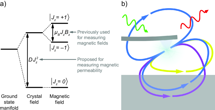
Figure 1: (a) The NV^- center’s ground state spin $J=1$ is split by the crystal field and magnetic field. Conventional NV^- magnetometry utilizes the splitting of the $|J_{z}=\pm 1\rangle$ states. We propose a way to measure magnetic response of materials using the splitting between the $|J_{z}=0\rangle$ and $|J_{z}=\pm 1\rangle$ states. (b) Implementation of magnetic-energy magnetometry. The spin of an NV^- center is located at the apex of a scanning probe tip, optically initialized (green) and detected (red). The spin’s magnetic induction (blue) is perturbed by the presence of the sample (gray), leading to modifications of the magnetic induction (diamagnetic, yellow; paramagnetic, purple).

Here we propose to overcome this disadvantage, by using the probe’s magnetic field to perturb the sample instead of relying on the sample’s magnetic field to perturb the probe. For any sample magnetic permeability differing from that of vacuum, the magnetic field of the probe will be dynamically altered, changing the magnetic energy stored in the probe’s magnetic field. For this approach, depicted in Fig. 1(b), we predict that for an NV^- center these changes in magnetic energy effectively translate into a modification of the crystal field splitting of the NV^- center’s spin ground state, see Fig. 1(a). Techniques have already been developed to measure small changes in this splitting for thermometry purposes Toyli et al. (2013); Kucsko et al. (2013); Neumann et al. (2013). Our calculations show that the magnetic energy approach to NV^--center magnetometry makes it possible to measure the magnetic permeabilities of diamagnetic and paramagnetic materials. For a unique application of this technique, we propose measuring the thickness of magnetically dead layers Sun et al. (1999). We show it is possible to determine this thickness with an accuracy superior to $0.1$ Å for experimentally realistic conditions.

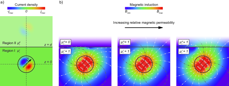
Figure 2: (a) A spin is placed in region I with relative magnetic permeability $\mu_{r}^{\text{I}}$, adjacent to a semi-infinite region II with $\mu_{r}^{\text{II}}$, filling the half-space $z>d$. The spin makes an angle $\eta$ with respect to the normal of the interface between the two regions. The color indicates the magnitude of the (image) current distribution for ${\cal P}(r)=\left[j_{0}(\pi r/R)\right]^{2}$, a spherical Bessel function of zeroth order, and $\mu_{r}^{\text{II}}=2$. (b) The calculated magnetic induction for the situation as described in (a). The magnetic induction near the interface is parallel to the interface for diamagnetic substances ($\mu_{r}^{\text{II}}=0$, left), though perpendicular to the interface for paramagnetic materials ($\mu_{r}^{\text{II}}\gg 1$, right). The magnitude of the magnetic induction is indicated by color, and its direction by the arrows of the streamlines.

Consider a spin with total angular momentum $J$ in region I, placed in close proximity to region II with a different magnetic permeability $\mu_{r}$ [see Fig. 2(a)]. In the absence of spin-orbit coupling, its magnetic moment density

$$\langle{\boldsymbol{\mu}}({\bf x})\rangle=\frac{2\mu_{B}}{\hbar}\langle{\bf J}({\bf x})\rangle=\frac{2\mu_{B}}{\hbar}\langle{\bf J}\rangle{\cal P}({\bf x}),$$ (1)

depends on its probability density ${\cal P}({\bf x})$, and the expectation value of the spin operator ${\bf J}=(J_{x},J_{y},J_{z})$; here $\mu_{B}$ is the Bohr magneton, and we took the $g$ factor to be $2$. In the Supplemental Material SM we show that this relation holds for any $N$-particle state, e.g., the complicated ground state of the NV^- center comprising 6 electrons Doherty et al. (2013). To simplify the calculation, we now treat the interaction of the spin’s magnetic moment with its environment classically; we will address its quantum-mechanical nature later on. The presence of a magnetic moment density requires a current density ${\bf j}({\bf x})=\nabla\times\langle{\boldsymbol{\mu}}({\bf x})\rangle$, which provides a direct expression for calculating, in the Coulomb gauge, the energy stored in a magnetic field Jackson (1998),

$$E_{\text{mag}}=\frac{1}{2}\int{\bf j}({\bf x})\cdot{\bf A}({\bf x})~{}d^{3}x.$$ (2)

Here ${\bf A}({\bf x})$ is the vector potential produced by ${\bf j}({\bf x})$. If ${\bf j}({\bf x})=0$ in region II, Eq. (2) determines the magnetic energy from ${\bf A}({\bf x})$ in region I alone. The effect of region II on the spin’s vector potential in region I can be included by replacing region II with an image current density Jackson (1998)

$$\widetilde{{\bf j}}({\bf x})=\frac{\mu_{r}^{\text{II}}-\mu_{r}^{\text{I}}}{\mu_{r}^{\text{II}}+\mu_{r}^{\text{I}}}\left(\begin{array}[]{r}j_{x}(x,y,2d-z)\\ j_{y}(x,y,2d-z)\\ -j_{z}(x,y,2d-z)\\ \end{array}\right)_{\hat{\bf x},\hat{\bf y},\hat{\bf z}},$$ (6)

where for simplicity we neglect any surface current at the interface between the regions. A treatment of surface currents would be required for conductive materials with a nonzero component of their magnetization parallel to the surface normal at the interface of the two regions. The image current generates a vector potential $\widetilde{{\bf A}}({\bf x})$; the total vector potential in region I is then ${\bf A}({\bf x})+\widetilde{{\bf A}}({\bf x})$.

For ease of calculation we assume isolated spin systems are approximately spherically symmetric and limited to a sphere with radius $R<d$. We will show later on that is a fair approximation for the NV^- center, even though that spin center has $C_{3v}$ symmetry Doherty et al. (2013). For a spin oriented such that its integrated magnetic moment makes an angle $\eta$ with respect to the $z$ axis [see Fig. 2(a)], the spin’s current density

$${\bf j}({\bf x}) =2\mu_{B}J\frac{d{\cal P}(r)}{dr}$$

$$\quad\times\left(\begin{array}[]{c}0\\ \sin\eta\sin\phi\\ \sin\eta\cos\theta\cos\phi-\cos\eta\sin\theta\end{array}\right)_{\hat{\bf r},\hat{\boldsymbol{\theta}},\hat{\boldsymbol{\phi}}},$$ (10)

for $r\leq R$. The vector potential resulting from this current distribution, calculated by expanding the Green’s function in spherical harmonics and performing several (partial) integrations, is

$${\bf A}({\bf x}) =-\frac{2\mu_{0}\mu_{r}^{\text{I}}\mu_{B}J}{r^{2}}\left(\int_{0}^{r}{\cal P}(r^{\prime})r^{\prime 2}dr^{\prime}\right)$$

$$\quad\times\left(\begin{array}[]{c}0\\ \sin\eta\sin\phi\\ \sin\eta\cos\theta\cos\phi-\cos\eta\sin\theta\end{array}\right)_{\hat{\bf r},\hat{\boldsymbol{\theta}},\hat{\boldsymbol{\phi}}},$$ (14)

for $r\leq R$, and the image current produces a vector potential

$$\widetilde{{\bf A}}({\bf x}) =\frac{\mu_{r}^{\text{II}}-\mu_{r}^{\text{I}}}{\mu_{r}^{\text{II}}+\mu_{r}^{\text{I}}}\left(\frac{\mu_{0}\mu_{r}^{\text{I}}\mu_{B}J}{2\pi\left(4d^{2}-4rd\cos\theta+r^{2}\right)^{3/2}}\right)$$

$$\times\left(\begin{array}[]{c}-2d\sin\eta\sin\theta\sin\phi\\ (r-2d\cos\theta)\sin\eta\sin\phi\\ (r\cos\theta-2d)\sin\eta\cos\phi+r\cos\eta\sin\theta\end{array}\right)_{\hat{\bf r},\hat{\boldsymbol{\theta}},\hat{\boldsymbol{\phi}}},$$ (18)

for $z<d$. These vector potentials determine the spin’s magnetic induction ${\bf B}({\bf x})=\nabla\times{\bf A}({\bf x})$, see Fig. 2(b). The magnetic induction is either repelled from (drawn to) region II if $\mu_{r}^{\text{II}}<\mu_{r}^{\text{I}}$ ($\mu_{r}^{\text{II}}>\mu_{r}^{\text{I}}$), as the magnetization in region II induced by the spin’s magnetic field is either antiparallel (diamagnetic) or parallel (paramagnetic) to the spin’s magnetic field.

Using Eq. (2) the magnetic energy

$$E_{\text{mag}}=\frac{16}{3} \mu_{0}\mu_{r}^{\text{I}}\mu_{B}^{2}\pi\int_{0}^{R}{\cal P}(r)^{2}r^{2}dr$$

$$+\left(\frac{\mu_{r}^{\text{II}}-\mu_{r}^{\text{I}}}{\mu_{r}^{\text{II}}+\mu_{r}^{\text{I}}}\right)\frac{\mu_{0}\mu_{r}^{\text{I}}\mu_{B}^{2}J^{2}}{32\pi d^{3}}\left[3+\cos 2\eta\right].$$ (19)

The first term is the magnetic energy of the spin itself, and is inversely proportional to $R^{3}$ (for ${\cal P}(r)=\left[j_{0}(\pi r/R)\right]^{2}$, a spherical Bessel function of zeroth order). The magnetic self-energy is experimentally inaccessible and goes to infinity for $R\rightarrow 0$, a well-known problem in classical electrodynamics Jackson (1998); Landau and Lifshitz (1971). The second term in Eq. (19) represents the change to the magnetic energy due to the presence of region II. These corrections are independent of ${\cal P}(r)$ due to the assumed spherical symmetry. The other dependencies of the magnetic energy are trivial to understand, after realizing that the change in magnetic energy depends on how much of the spin’s magnetic induction penetrates region II. The magnitude of the angular variation of the magnetic energy for $d=1$ nm is of the order of 10 neV (or 0.2 mK), which is extremely challenging to measure by spectroscopy. Also, the resulting force ${\bf F}=-\nabla E_{\text{mag}}\approx$ aN exerted on the scanning probe would be difficult to detect by atomic force microscopy. Instead, we will show that the magnetic energy can be probed using a coherent measurement of an NV^- center’s spin.

The ground state of an NV’s spin $J=1$ is effectively described using the Hamiltonian ${\cal H}_{\text{NV}}=D_{\text{GS}}J_{z}^{2}$, where $D_{\text{GS}}\approx 2.87$ GHz is the fine-structure constant due to the crystal field, and the $z$ direction is the NV^- center’s symmetry axis Doherty et al. (2013), see Fig. 1(a). To compare the NV^--center spin with the spin considered in Fig. 2(a), it is convenient to orient the NV^- center’s symmetry axis perpendicular to the interface between the two regions. It has recently been demonstrated that such orientation can be realized deterministically in practice Michl et al. (2014). Analogous to the spin considered in Fig. 2(a), the NV^- center’s spin is placed in the superposition $|J_{\eta}\rangle=\cos^{2}\left(\eta/2\right)|+1\rangle+\tfrac{1}{2}\sqrt{2}\sin\eta|0\rangle+\sin^{2}\left(\eta/2\right)|-1\rangle$, such that the expectation value of the spin makes an angle $\eta$ with respect to the $z$ axis. The energy of this state

$$\langle J_{\eta}|{\cal H}_{\text{NV}}|J_{\eta}\rangle=\frac{D_{\text{GS}}}{4}\left[3+\cos 2\eta\right]$$ (20)

is identical to the angular dependence of the magnetic energy in Eq. (19). Therefore the effect of a nearby region with different magnetic permeability on the spin of an NV^- center seems to effectively change its fine-structure constant.

A fully quantum-mechanical treatment of the spin results in the magnetic energy Hamiltonian (see Supplemental Material SM )

$${\cal H}_{\text{mag}}=\left(\frac{\mu_{r}^{\text{II}}-\mu_{r}^{\text{I}}}{\mu_{r}^{\text{II}}+\mu_{r}^{\text{I}}}\right)\frac{\mu_{0}\mu_{r}^{\text{I}}\mu_{B}^{2}}{16\pi\hbar^{2}d^{3}}J_{z}^{2}=D_{\text{mag}}J_{z}^{2},$$ (21)

so that the NV^- center effectively has $D=D_{\text{GS}}+D_{\text{mag}}$. Since the magnetization induced in region II depends on the spin and acts back on the spin itself, ${\cal H}_{\text{mag}}$ depends on the spin squared. In the Supplemental Material SM we show that ${\cal H}_{\text{mag}}$ has a similar structure when ${\cal P}({\bf x})$ has cylindrical symmetry and its axial symmetry axis is perpendicular to the interface between regions I and II. We also calculated that cylindrical symmetry changes an NV^- center’s $D_{\text{mag}}$ by $\leq 5\%$ from the spherical approximation. Lowering the symmetry further to NV^-’s $C_{3v}$ symmetry leads to additional small corrections, which we estimate to be less than $20\%$ for an NV^- center 1 nm away from the interface. Assuming a spherical ${\cal P}({\bf x})$ is therefore a reasonable approximation. Note that in the classical limit $J\rightarrow\infty$ we get $\langle J_{\eta}|{\cal H}_{\text{mag}}|J_{\eta}\rangle=E_{\text{mag}}$, and also there is no effect for $J=\tfrac{1}{2}$.

The following (briefly outlined) coherent measurement protocol can be used to sensitively measure $D$; more details can be found in Ref. Toyli et al. (2013). The NV^- center is first prepared in the $|J_{z}=0\rangle$ state using a pulsed optical excitation, by making use of the spin-dependent decay from the excited state manifold to the ground state manifold Doherty et al. (2013). The spin is then placed in a superposition of the $|J_{z}=0\rangle$ and $|J_{z}=\pm 1\rangle$ states using a ${\pi}/{2}$ microwave pulse at frequency $D$. This superposition will acquire a phase $\exp({-iD\tau})$ after a free evolution time $\tau$. By applying another ${\pi}/{2}$ microwave pulse to project the spin onto the $|J_{z}=0\rangle$ state, the phase can be determined by optical measurement of the $|J_{z}=0\rangle$ population; $D$ follows from measuring the phase as function of $\tau$, most accurately through the use of a reference oscillator. The spin will experience decoherence during its free evolution; this can be mitigated using dynamic decoupling protocols, which can be designed to optimize the sensitivity at which $D$ can be measured Toyli et al. (2013).

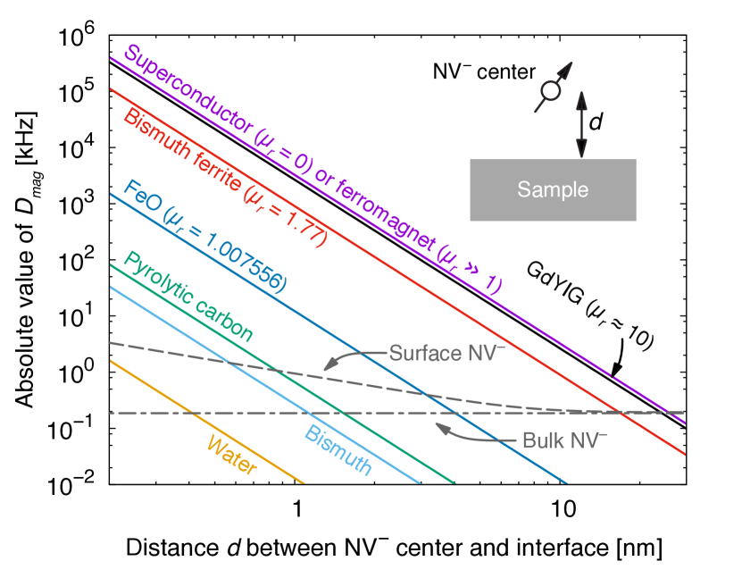
Figure 3: The magnetic energy contribution $D_{\text{mag}}$ to the fine-structure constant as function of the distance $d$ between the NV^- center and the sample, for samples having different magnetic permeabilities. The grey lines indicate the measurable change in $D$ for a measurement time of $100$s, reported for a bulk NV^- center (dot-dash) and estimated for surface NV^- centers (dash); see text for details. We took the low-frequency values for $\mu_{r}$ and assumed the superconductor to be a perfect diamagnet (i.e., vanishing penetration depth). The $\mu_{r}$ of pyrolytic carbon, bismuth, and water are, respectively, 0.999590, 0.999834, and 0.999992.

In Fig. 3 we show how $D_{\text{mag}}$ depends both on the distance $d$ between the NV^- center and the sample, and on the relative magnetic permeability of the sample. Diamond itself has a very weak diamagnetic response, $\mu_{r}=1-2.2\times 10^{-5}$ Haynes (2015), and has no free carriers. The NV^- center is therefore in practice magnetically insensitive to its host, and $D_{\text{mag}}$ is barely affected by the diamond’s shape. Using a coherent measurement technique, $D$ has been measured with a sensitivity of $1.85~{}\text{kHz}/\sqrt{\text{Hz}}$ Toyli et al. (2013). Assuming a measurement time of 100 s, changes in $D$ of 0.2 kHz can therefore be detected for a bulk NV^- center. From Fig. 3 it appears possible to detect both paramagnetic and diamagnetic substances if the NV^- center is a few nm away from the sample. Such small distances are conventional in scanning probe microscopy Seo and Jhe (2008), and have been achieved in conventional NV^--center magnetometry Loretz et al. (2014). Recent studies showed that the proximity of the surface lowers the NV^- center’s $T_{2}$ coherence time due to a surface electronic spin bath and/or a surface phonon-related mechanism Rosskopf et al. (2014); Myers et al. (2014); Romach et al. (2015). This increases the minimal detectable change in $D$ by a factor $\sqrt{T_{2}^{\text{bulk}}/T_{2}^{\text{surface}}}$ Toyli et al. (2013). Based on the experimental data of Ref. Romach et al. (2015), we roughly estimated the dependence of this ratio on $d$. We included in Fig. 3 both the minimal detectable change in $D$ estimated for near-surface and reported for bulk NV^- centers for a measurement time of $100$ s. Increasing $T_{2}$ (potentially by mitigating the surface phenomena by surface passivation), improving sensing schemes, or extending the measurement time would push the minimal detectable change in $D$ down.

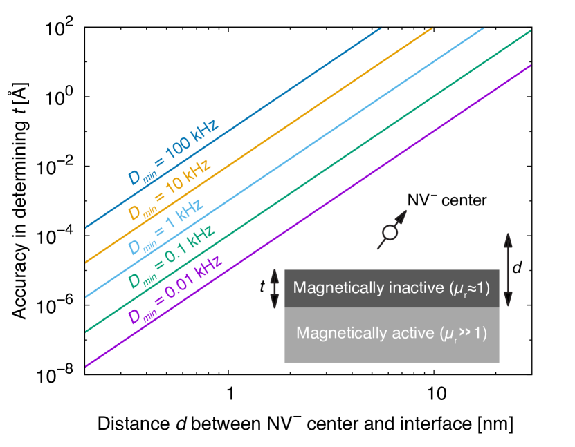
Figure 4: The accuracy at which the thickness $t$ of a magnetically dead layer ($\mu_{r}$ is about 1) can be determined, as a function of the distance $d$ between the NV^--center and the magnetically active region ($\mu_{r}\gg 1$), for different minimal detectable changes $D_{\text{min}}$. Based on Ref. Toyli et al., 2013, $D_{\text{min}}=0.2$ kHz for a bulk NV^--center and a measurement time of 100s. See Fig. 3 and its discussion in the text to determine an estimated $D_{\text{min}}$ close to the surface.

Our analysis is not limited to NV^- centers; any spin close to a region with different magnetic permeability will experience an orientation-dependent magnetic energy, which affects its dynamics. Therefore the spins of other promising color centers Gordon et al. (2013), notably the divacancy in SiC, could also be used to detect the magnetic properties of nearby materials. Such systems would preferably have a smaller fine-structure constant $D_{\text{GS}}$, since in the proposed measurement scheme the NV^- center’s spin is precessing at that frequency. Although this does not impede the effect of the magnetic energy on the fine-structure constant, it does set the frequency at which the magnetic properties of the sample are probed; lowering this frequency would be favorable. Alternatively, different measurement schemes could be developed, which remove the necessity of the spin precessing at such frequencies.

As an example of the added value of the proposed magnetic-energy-based magnetometry, we suggest to use this technique to measure the thickness $t$ of magnetically dead layers Sun et al. (1999). A common problem in magnetic multilayered materials, such as magnetic tunnel junctions Ikeda et al. (2010), is the magnetic inactivity of the top surface layer of the structure, see inset of Fig. 4. We can make use of the strong distance dependence of the magnetic energy ($E_{\text{mag}}\propto d^{-3}$) to sensitively determine the distance $d$ between the NV^- center and the boundary of the magnetically active material. As the separation between the NV^- center and the physical boundary of the sample is known through calibration, the thickness $t$ of the magnetically inactive material can be determined with high precision. Figure 4 predicts that this can be achieved with remarkable accuracy.

We propose a method to sense the magnetic properties of materials based on the magnetic energy of a nearby spin. This method inverts the conventional scheme of scanning-probe magnetometers, making it possible to sense materials which have no natural magnetic field external to their volume. This scheme can be applied to NV^- centers and, using realistic assumptions, we predict it should be possible to detect both para- and diamagnetic materials. Future theoretical work towards implementing different color centers or different measurement schemes could lower the frequency at which the magnetic properties are probed and improve the predicted sensitivity.

The authors acknowledge support from an Air Force Office of Scientific Research (AFOSR) Multidisciplinary University Research Initiative (MURI) Grant and J. v. B. acknowledges a Rubicon Grant from the Netherlands Organization for Scientific Research.

References

- Rabi et al. (1938) I. I. Rabi, J. R. Zacharias, S. Millman, and P. Kusch, Phys. Rev. 53, 318 (1938).
- Jaklevic et al. (1964) R. C. Jaklevic, J. Lambe, A. H. Silver, and J. E. Mercereau, Phys. Rev. Lett. 12, 159 (1964).
- Wehrli (1992) F. W. Wehrli, Phys. Today 45, 34 (1992).
- Balasubramanian et al. (2008) G. Balasubramanian, I. Y. Chan, R. Kolesov, M. Al-Hmoud, J. Tisler, C. Shin, C. Kim, A. Wojcik, P. R. Hemmer, A. Krueger, T. Hanke, A. Leitenstorfer, R. Bratschitsch, F. Jelezko, and J. Wrachtrup, Nature (London) 455, 648 (2008).
- Ciobanu et al. (2002) L. Ciobanu, D. Seeber, and C. Pennington, J. Magn. Reson. 158, 178 (2002).
- Glover and Mansfield (2002) P. Glover and S. P. Mansfield, Rep. Prog. Phys. 65, 1489 (2002).
- Martin and Wickramasinghe (1987) Y. Martin and H. K. Wickramasinghe, Appl. Phys. Lett. 50, 1455 (1987).
- Chang et al. (1992) A. M. Chang, H. D. Hallen, L. Harriott, H. F. Hess, H. L. Kao, J. Kwo, R. E. Miller, R. Wolfe, J. van der Ziel, and T. Y. Chang, Appl. Phys. Lett. 61, 1974 (1992).
- Degen et al. (2009) C. L. Degen, M. Poggio, H. J. Mamin, C. T. Rettner, and D. Rugar, Proc. Natl. Acad. Sci. U.S.A. 106, 1313 (2009).
- Hong et al. (2013) S. Hong, M. S. Grinolds, L. M. Pham, D. Le Sage, L. Luan, R. L. Walsworth, and A. Yacoby, MRS Bull. 38, 155 (2013).
- van Oort et al. (1988) E. van Oort, N. B. Manson, and M. Glasbeek, J. Phys. C 21, 4385 (1988).
- Childress et al. (2006) L. Childress, M. V. G. Dutt, J. M. Taylor, A. S. Zibrov, F. Jelezko, J. Wrachtrup, P. R. Hemmer, and M. D. Lukin, Science 314, 281 (2006).
- Maze et al. (2008) J. R. Maze, P. L. Stanwix, J. S. Hodges, S. Hong, J. M. Taylor, P. Cappellaro, L. Jiang, M. V. G. Dutt, E. Togan, A. S. Zibrov, A. Yacoby, R. L. Walsworth, and M. D. Lukin, Nature (London) 455, 644 (2008).
- Toyli et al. (2013) D. M. Toyli, C. F. de las Casas, D. J. Christle, V. V. Dobrovitski, and D. D. Awschalom, Proc. Natl. Acad. Sci. U.S.A. 110, 8417 (2013).
- Kucsko et al. (2013) G. Kucsko, P. C. Maurer, N. Y. Yao, M. Kubo, H. J. Noh, P. K. Lo, H. Park, and M. D. Lukin, Nature (London) 500, 54 (2013).
- Neumann et al. (2013) P. Neumann, I. Jakobi, F. Dolde, C. Burk, R. Reuter, G. Waldherr, J. Honert, T. Wolf, A. Brunner, J. H. Shim, D. Suter, H. Sumiya, J. Isoya, and J. Wrachtrup, Nano Lett. 13, 2738 (2013).
- Sun et al. (1999) J. Z. Sun, D. W. Abraham, R. A. Rao, and C. B. Eom, Appl. Phys. Lett. 74, 3017 (1999).
- (18) See Supplemental Material for the derivation of the spin density of an -particle state [validating Eq. (1)], and for the derivation of the magnetic energy Hamiltonian treating the spin fully quantum mechanically and assuming a spherically or cylindrically symmetric probability density. The Supplemental Material includes Refs. Schwabl (2004); Bjorken and Drell (1965); Gali et al. (2008).
- Doherty et al. (2013) M. W. Doherty, N. B. Manson, P. Delaney, F. Jelezko, J. Wrachtrup, and L. C. L. Hollenberg, Phys. Rep. 528, 1 (2013).
- Jackson (1998) J. D. Jackson, Classical Electrodynamics, 3rd ed. (Wiley, New York, 1998).
- Landau and Lifshitz (1971) L. D. Landau and E. M. Lifshitz, The Classical Theory of Fields, 3rd ed., Landau and Lifshitz Course of Theoretical Physics - Vol. 2 (Pergamon Press, Oxford, 1971).
- Michl et al. (2014) J. Michl, T. Teraji, S. Zaiser, I. Jakobi, G. Waldherr, F. Dolde, P. Neumann, M. W. Doherty, N. B. Manson, J. Isoya, and J. Wrachtrup, Appl. Phys. Lett. 104, 102407 (2014).
- Haynes (2015) W. M. Haynes, Handbook of Chemistry and Physics (CRC, Cleveland, 2015).
- Seo and Jhe (2008) Y. Seo and W. Jhe, Rep. Prog. Phys. 71, 016101 (2008).
- Loretz et al. (2014) M. Loretz, S. Pezzagna, J. Meijer, and C. L. Degen, Appl. Phys. Lett. 104, 033102 (2014).
- Rosskopf et al. (2014) T. Rosskopf, A. Dussaux, K. Ohashi, M. Loretz, R. Schirhagl, H. Watanabe, S. Shikata, K. M. Itoh, and C. L. Degen, Phys. Rev. Lett. 112, 147602 (2014).
- Myers et al. (2014) B. A. Myers, A. Das, M. C. Dartiailh, K. Ohno, D. D. Awschalom, and A. C. Bleszynski Jayich, Phys. Rev. Lett. 113, 027602 (2014).
- Romach et al. (2015) Y. Romach, C. Müller, T. Unden, L. J. Rogers, T. Isoda, K. M. Itoh, M. Markham, A. Stacey, J. Meijer, S. Pezzagna, B. Naydenov, L. P. McGuinness, N. Bar-Gill, and F. Jelezko, Phys. Rev. Lett. 114, 017601 (2015).
- Gordon et al. (2013) L. Gordon, J. R. Weber, J. B. Varley, A. Janotti, D. D. Awschalom, and C. G. Van de Walle, MRS Bull. 38, 802 (2013).
- Ikeda et al. (2010) S. Ikeda, K. Miura, H. Yamamoto, K. Mizunuma, H. D. Gan, M. Endo, S. Kanai, J. Hayakawa, F. Matsukura, and H. Ohno, Nat. Mater. 9, 721 (2010).
- Schwabl (2004) F. Schwabl, Advanced Quantum Mechanics (Springer, New York, 2004).
- Bjorken and Drell (1965) J. D. Bjorken and S. D. Drell, Relativistic Quantum Fields (McGraw-Hill, New York, 1965).
- Gali et al. (2008) A. Gali, M. Fyta, and E. Kaxiras, Phys. Rev. B 77, 155206 (2008).