A study on missing lines in the synthetic solar spectrum near the Ca triplet
Synthetic stellar spectra are extensively used for many different applications in astronomy, from stellar studies (such as in the determination of atmospheric parameters of observed stellar spectra), to extragalactic studies (e.g. as one of the main ingredients of stellar population models). One of the main ingredients of synthetic spectral libraries are the atomic and molecular line lists, which contain the data required to model all the absorption lines that should appear in these spectra. Although currently available line lists contain millions of lines, a relatively small fraction of these lines have accurate derived or measured transition parameters. As a consequence, many of these lines contain errors in the electronic transition parameters that can reach up to 200%. Furthermore, even for the Sun, our closest and most studied star, state-of-the-art synthetic spectra does not reproduce all the observed lines, indicating transitions that are missing in the line lists of the computed synthetic spectra. Given the importance and wide range of applications of these models, improvement of their quality is urgently necessary. In this work we catalogued missing lines in the atomic and molecular line lists used for the calculation of the synthetic spectra in the region of GAIA, comparing a solar model computed via a recent line list with a high quality solar atlas available in the literature. After that, we attempted the calibration of their atomic parameters with the code ALLiCE; the calibrated line parameters are publicly available for use.
Key Words.:
synthetic spectra, Sun, atomic line lists, atomic parameters, missing lines1 Introduction
Synthetic stellar spectra are extensively used in many different applications in astronomy, from the determination of atmospheric parameters of observed stellar spectra to the study of galaxy integrated spectra (as one of the main ingredients of stellar population models). Generating an accurate synthetic stellar spectrum requires the thermodynamic description of the atmosphere as a function of depth (e.g. Kurucz 1993; Castelli & Kurucz 2004; Paxton et al. 2011), the so-called model atmosphere. These model atmospheres may include simplifications for complex physical process, such as convection, or computational limitations, for example, geometry and/or boundary conditions; often they depend on incomplete or imprecise atomic and molecular opacities (Czekala et al. 2015).
To generate the synthetic stellar spectra, a stellar synthesis code (e.g. SYNTHE; Kurucz & Avrett 1981) solves the radiative transfer of a given model atmosphere using an atomic and molecular line list. Atomic and molecular opacities also greatly affect the radiative transfer in stars and consequently their physical structure. Despite this, we are far away from having complete and accurate line lists and, in fact, half of the known lines in the stellar spectra are not present in the line lists with wavelengths considered to have good accuracy (Kurucz 2011). Besides, detailed spectral models calibrated to a single star (like Sun or Vega) are very important but, at the same time, rare and poorly tested (e.g. Czekala et al. 2015).
In recent decades, there were great efforts to complete and improve the line lists and nowadays there are large atomic databases (e.g. National Institute of Standards and Technology-Atomic Spectra Database111http://www.nist.gov/ and Vienna Atomic Line Database222http://vald.astro.uu.se).
Although the current line lists include millions of absorption lines, only a small fraction of these lines were actually accurately measured in laboratory or have accurate parameters derived, and the uncertainty in the transition parameters for atomic lines can reach up to 200%. Even for the Sun, our closest and most studied star, the synthetic spectrum still does not completely reproduce all the features and many of the lines are missing in the synthetic spectrum (Kurucz 2011). For the purpose of spectrophotometric studies, the missing lines have been included via the so-called “predicted lines”, in which, rather than measured, one or both energy levels of the transition was only predicted through quantum mechanics calculations (Kurucz 1992). These lines are essential to better describe the structure of atmospheric models and for spectrophotometric forecasts (e.g. Short & Lester 1996; Coelho 2014). However, these quantum mechanical predictions are accurate only at a few percent level and the wavelength of these lines can be largely incorrect. As such, the inclusion of the predicted lines is inappropriate to generate theoretical stellar spectra with high resolution (e.g. Bell et al. 1994; Castelli & Kurucz 2004; Munari et al. 2005). As a consequence of this complex scenario, synthetic libraries are only partially able to reproduce observed spectra and the quality of the model varies with spectral type and wavelength range modelled (e.g. Bertone 2006; Bertone et al. 2008; Martins & Coelho 2007; Coelho 2014).
In an attempt to fill this gap, many groups have been working through the years to improve the quality of atomic data used to generate synthetic spectra, focusing on reducing the uncertainty of the transition probabilities (e.g. Taklif 1990; Klose et al. 2002; Fuhr & Wiese 2006; Safronova et al. 2010; Bacławski 2011; Pickering et al. 2011; Wiese et al. 2011; Civiš et al. 2012; Ruffoni et al. 2013) and the broadening parameters (e.g. Anstee & O’Mara 1995; Barklem & O’Mara 1997; Barklem et al. 1998; Lesage et al. 1999; Barklem et al. 2000; Klose et al. 2002; Derouich et al. 2003; Dimitrijević et al. 2003). Besides, many limitations of these atomic line lists have been approached by different methods and authors, mainly aimed at chemical analyses of stellar photospheres using high resolution spectra (e.g. Stalin et al. 1997; Blackwell-Whitehead et al. 2008; Borrero et al. 2003; Jorissen 2004; Den Hartog et al. 2011; Shchukina & Vasil’eva 2013; Wood et al. 2013). However, not only known lines have to be improved, but the identification of missing lines is necessary to fill significant gaps that are poorly modelled in stellar spectra.
In this work, we identify and catalogue missing lines in the atomic and molecular line lists used to generate synthetic spectra of the Sun based on a recent line list available in literature, and, when possible, calibrate the atomic lines. For this task we used an observed solar spectrum (Wallace et al. 2011), which is an obvious choice since it is the highest quality observed stellar spectrum available in the literature. Additionally, uncertainties involved in the determination of its effective temperature, superficial gravity, chemical abundance, etc. are smaller than for any other star. The identification of missing lines was performed in the wavelength range from since it is the spectral region covered by the Radial-Velocity Spectrometer on the GAIA telescope (Lindegren & Perryman 1996; Mignard 2005) launched in 2013. Even though the spectral resolution of the mentioned instrument is relatively low ( 11500 ), we can expect this wavelength region to be highly attractive to stellar and galactic studies for the years to come. We used the observed solar spectrum available from Wallace et al. (2011) and compared with the synthetic spectrum generated using the atomic and molecular line list from (Sbordone et al. 2004), updated by Coelho (2014). We use the code ALiCCE (Atomic Lines Calibration using the Cross-Entropy Algorithm; Martins et al. 2014) to calibrate the atomic parameters.
This paper is structured as follows: in Section 2, we give details about the observed solar spectrum used in this work; in Section 3 we present the identification and characterisation of the missing lines in the synthetic solar spectrum; in Section 4 we show the calibration of the atomic parameters of some of these lines; and, in Section 5, we present our discussion and conclusions.
2 The observed solar spectrum
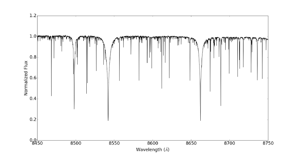
High resolution spectral atlases of the Sun have been produced since the middle of the 20th century (e.g. Minnaert et al. 1940). However, most of the solar spectral atlases are of disk-centre regions. The solar flux spectra, taken over the integrated disk, are much less common. A flux atlas shows the mean effects of rotation, convection, and centre-to-limb variation. Thus, flux spectra are fundamental for comparisons with other stellar spectra and with synthetic spectra (Wallace et al. 2011).
The observed solar spectrum used in this work was published by Wallace et al. (2011). These authors claim that the quality of their spectrum is higher than Kurucz (2005) because of the more efficient subtraction of the telluric lines. The observation was taken at McMath-Pierce Solar Telescope, located on Kitt Peak, using the Fourier Transform Spectrograph (hereafter FTS). The solar integrated light FTS spectra were obtained mainly on two occasions: in 1980–1981 for Kurucz et al. (1984) atlas and in 1989 for monitoring the irradiance spectrum over the solar cycle (Mitchell & Livingston 1991). Both sets were observed near the peaks of sunspot activity. These were the data used by Wallace et al. (2011) to produce a new flux atlas.
The wavelength coverage of this observed spectrum ranges from and the spectral resolution varies from 350 000 to 700 000 (). The signal to noise in the continuum goes beyond several hundreds. In principle, the FTS could have observed the entire spectral region in a single integration, however, to reduce the photon noise, six separate observations were carried out with the spectral coverage in each limited by optical bandpass filters. The Doppler shift correction was determined empirically by measuring the solar Fe i line positions and correcting them to the frequencies in Nave et al. (1994). Thus, the solar gravitational redshift was also removed from the wave number scales.
Wallace et al. (2011) made the telluric emission correction, knowing that from the solar spectrum is free from any terrestrial lines. However, weak lines of begin to appear from and lines also appear from . The scheme developed by Wallace et al. (2011) to correct for the telluric spectrum was to use the solar spectra obtained from many sets with different air masses, in the morning or evening, applied to the disk-centre spectra. This was carried out because the flux spectra were not taken in suitable airmass sets to allow the transmission spectra to be extracted. They found the best signal to noise and correction with the flux spectrum from October 1989, using a disk-centre observation from July 1983.
More details about the observations and the reduction processes are available in Wallace et al. (2011). Figure 1 shows the Wallace et al. (2011) spectrum for the spectral region used in this work.
3 Line identifications
We used the solar model atmosphere from Castelli & Kurucz (2004), which is based in ATLAS9 (Kurucz 1970; Sbordone et al. 2004), to generate the synthetic spectrum of the Sun. There are two different downloadable atmosphere models: one using the Asplund et al. (2005) chemical abundances and another using the Grevesse & Sauval (1998) 333http://wwwuser.oats.inaf.it/castelli/sun.html. Both are tested in this work. The effective temperature of the Sun considered is 5777 K, the surface gravity is 4.44 (Kurucz 1970) and convection was taken into account. We chose ATLAS9 because it is a static and local thermodynamic equilibrium atmosphere model and is still one of the most commonly used models for chemical abundances studies to generate synthetic stellar libraries, and it reproduces well the colours of observed stars (Martins & Coelho 2007).
To generate the synthetic spectrum, we used the SYNTHE code (Kurucz & Avrett 1981) in its Linux version published by Sbordone et al. (2004). The atomic and molecular line lists used are publicly available with ATLAS9 and were updated according to Coelho (2014). The spectral synthesis code uses the atomic and molecular line lists to solve the equation of radiative transfer. The parameters necessary for the calculation of each absorption line are the central wavelength, the energy of the upper and lower levels, the oscillator strength, and the broadening parameters (natural, Stark and Van der Waals). The broadening parameters dominate the line wings, while the oscillator strengths dominate the line depths. The spectral resolution adopted for this work, given by , was 676000, which is the same resolution of the observed spectrum in this region. To reproduce the line broadening from the solar rotational velocity, we applied a rotational velocity () of 2.4 (Smith 1978) and microturbulence of 1.0 .
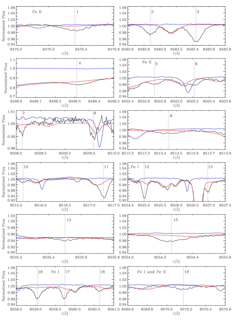
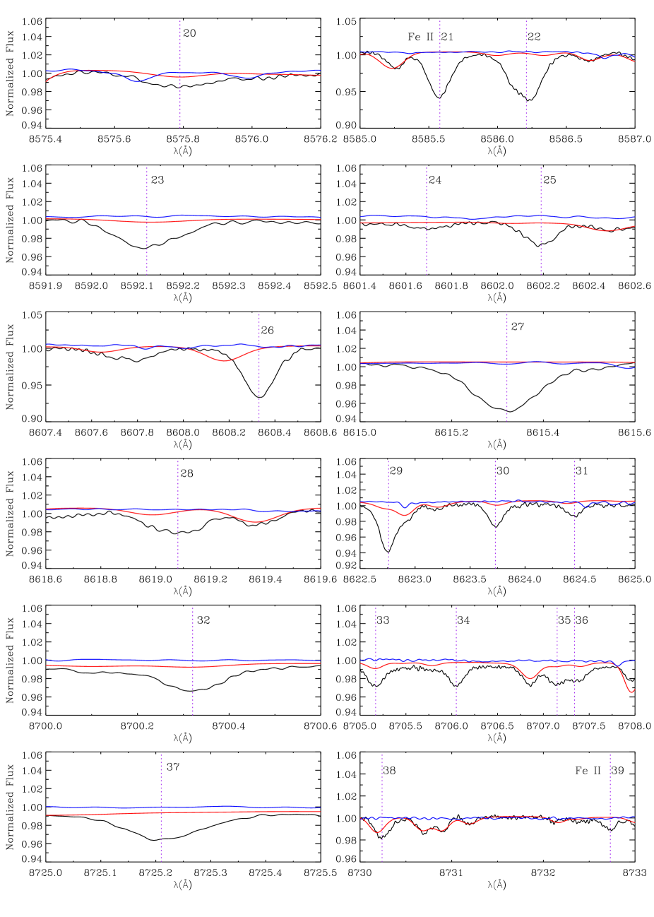
We produced synthetic spectra for three different chemical abundances: Asplund et al. (2005) and Grevesse & Sauval (1998), whose model atmosphere were downloaded from the website of F. Castelli as indicated above, and Asplund et al. (2009). To produce a synthetic solar spectrum with the latest abundances we used the same model atmosphere as with Asplund et al. (2005) abundances, but changing abundances in SYNTHE code accordingly. This approach is valid for small variations in the chemical abundances, which should not significantly change the atmosphere structure. The three different abundances were tested just to ensure that weak missing lines were not just an artefact of small abundance changes. The comparison between the spectra was carried out visually over the entire spectral range studied to identify the missing lines in the theoretical spectrum. The telluric spectrum used for the correction of the solar spectrum was also inspected to avoid the classification of possible residual subtractions as missing lines.
All lines in this wavelength range that were present in the observed spectrum and absent in the theoretical spectrum have been identified and catalogued. We found 39 missing lines in the wavelength range analysed. For the characterisation of these lines, each one was fitted by a Gaussian profile. Wallace et al. (2011) also identified some lines in the spectrum of the Sun and therefore we compared our catalogued lines with the lines identified by these authors. Table 1 shows the central wavelength values of the catalogued lines, their identification by Wallace et al. (2011) (when present), the equivalent width (EW), the full width at half maximum (FWHM), and the asymmetry of each line. Figures 2 and 3 show each of the missing lines identified.
| Wallace et al. | (Å) | EW (Å) | FWHM | asymmetry | |
|---|---|---|---|---|---|
| 1 | Cr ii | 8470.36 | 0.0036 | 2.747 | -0.259 |
| 2 | Fe i | 8482.88 | 0.0046 | 2.309 | -0.130 |
| 3 | - | 8483.44 | 0.0078 | 2.379 | -0.274 |
| 4 | CN red | 8499.30 | 0.0179 | 3.311 | 0.003 |
| 5 | - | 8502.73 | 0.0192 | 5.581 | 0.851 |
| 6 | CN red | 8503.22 | 0.0042 | 6.556 | 1.034 |
| 7 | - | 8508.12 | 0.0008 | 1.564 | -0.138 |
| 8 | - | 8509.59 | 0.0025 | 2.431 | 0.173 |
| 9 | - | 8513.45 | 0.0029 | 3.122 | 0.099 |
| 10 | - | 8515.65 | 0.0016 | 2.156 | -0.182 |
| 11 | - | 8517.29 | 0.0130 | 3.040 | 0.651 |
| 12 | Fe i | 8525.01 | 0.0096 | 2.180 | -0.193 |
| 13 | - | 8526.96 | 0.0073 | 2.714 | 0.317 |
| 14 | - | 8535.50 | 0.0011 | 1.977 | -0.047 |
| 15 | - | 8554.27 | 0.0707 | 8.576 | 0.679 |
| 16 | Co i | 8559.05 | 0.0051 | 2.502 | -0.129 |
| 17 | Fe i | 8559.74 | 0.0052 | 2.271 | 0.008 |
| 18 | - | 8560.64 | 0.0079 | 4.084 | 0.579 |
| 19 | - | 8570.17 | 0.0016 | 2.406 | 0.317 |
| 20 | CN red | 8575.79 | 0.0129 | 5.960 | 0.657 |
| 21 | S i | 8585.58 | 0.0106 | 2.642 | -0.228 |
| 22 | - | 8586.21 | 0.0195 | 4.114 | -0.007 |
| 23 | Fe i | 8592.12 | 0.0053 | 2.476 | 0.053 |
| 24 | - | 8601.69 | 0.0093 | 6.157 | 0.530 |
| 25 | - | 8602.19 | 0.0043 | 2.442 | 0.082 |
| 26 | - | 8608.33 | 0.0111 | 2.362 | -0.466 |
| 27 | - | 8615.32 | 0.0080 | 2.335 | -0.468 |
| 28 | CN red | 8619.08 | 0.0075 | 3.992 | 0.254 |
| 29 | CN red | 8622.75 | 0.0075 | 2.242 | -0.129 |
| 30 | - | 8623.73 | 0.0043 | 2.218 | -0.427 |
| 31 | - | 8624.45 | 0.0021 | 2.162 | -0.141 |
| 32 | Fe i | 8700.32 | 0.0039 | 2.254 | -0.860 |
| 33 | - | 8705.17 | 0.0035 | 2.631 | -0.154 |
| 34 | - | 8706.06 | 0.0035 | 2.594 | -0.143 |
| 35 | Mg i | 8707.15 | 1.3182 | 26.072 | 0.827 |
| 36 | Cr i | 8707.34 | 1.7846 | 35.624 | 1.73 |
| 37 | - | 8725.21 | 0.0046 | 2.383 | -0.376 |
| 38 | CN red | 8730.25 | 0.0037 | 2.855 | -0.099 |
| 39 | - | 8732.72 | 0.0013 | 2.281 | 0.099 |
We can see in Table 1 that about half of the lines (21 lines) have widths of about 2.4 , which correspond to the net effect of rotational velocity, microturbulence, and macroturbulence in the Sun444 A significant contribution to the spectral line broadening might come from velocity fields in the stellar photosphere. In 1D model atmospheres these velocity fields are represented by microturbulence and macroturbulence, although physically they have little to do with turbulence (Doyle et al. 2014).. We assume that the broadening of these lines is dominated by these listed combined effects, rather than an effect intrinsic of the lines. We can also speculate that these lines are produced or dominated by one atomic transition as opposed to molecular transitions or a blend of lines. Another reason that these lines are produced or dominated by only one electronic transition is their symmetry. Asymmetric lines are more likely produced by a blend of lines, whether atomic or molecular. The asymmetry was measured through the skewness of the line, where values close to zero mean very symmetrical distributions. Thirteen of these lines have asymmetry values close to zero (lines 2, 8, 10, 12, 16, 17, 23, 25, 29, 31, 33, 34, and 39). For these lines, —asymmetry— ¡0.20. However, line 29 was identified by Wallace et al. (2011) as due to a CN transition, so we cannot rule out that some of these lines come from molecular transitions. Another caveat that might be taken into account is that asymmetries and wavelength shifts in stars might be correlated with convection in the sense that warm, rising convective elements are blueshifted and cool and falling convective elements are redshifted. However, according to Dravins et al. (1998) this effect in the Sun is around 300 m/s, which is much smaller than visible asymmetries seen here. For the value of the central wavelength, this implies in a of 0.0085 Å at 8500 Å, which is also minor for the values observed here. Signatures with much larger widths are more likely to be produced by a blend of lines, although single atomic lines can be broadened by hyperfine and isotopic splitting. (Wahlgren 2005). Two signatures have widths that are smaller than 2.0 (lines 7 and 14). This is possibly due to measurement errors caused by the difficulty of adjusting these signatures, which are in regions with a high density of lines.
After characterising each signature, we looked for the atomic data of these missing lines in the NIST database to verify whether their absence was not only a matter of outdated line lists. The atomic data collected from NIST were measured in the laboratory. Table 5 shows the relation between catalogued missing lines and the data found in NIST.
| (Å) | (Å) | Element | log gf | Element Code | Quality | |||
| 1 | 8470.36 | 8470.37 | Fe ii | -2.5 | 54275.649 | 66078.272 | 26.01 | D |
| 2 | 8482.88 | 8482.67 | Ho i | - | - | - | 67.00 | - |
| 2 | 8482.88 | 8482.684 | Sc ii | - | 66048.39 | 77833.88 | 21.01 | - |
| 3 | 8483.44 | 8483.39 | Mo i | - | - | - | 42.00 | - |
| 3 | 8483.44 | 8483.56 | Ru i | - | 32391.95 | 44176.23 | 44.00 | - |
| 4 | 8499.30 | 8499.34a𝑎aa𝑎aPrivate communication from Gillian Nave (NIST) | Fe i | - | - | - | 26.00 | - |
| 5 | 8502.73 | 8502.7 | Tb i | - | - | - | 65.00 | - |
| 5 | 8502.73 | 8502.714 | Fe ii | - | 92116.529 | 103874.261 | 26.01 | - |
| 5 | 8502.73 | 8502.714 | Fe ii | - | 93328.553 | 105086.265 | 26.01 | - |
| 6 | 8503.22 | 8503.212 | Co ii | -0.14 | 97062.844 | 108819.860 | 27.01 | C+ |
| 7 | 8508.12 | 8508.08 | Lu i | - | - | - | 71.00 | - |
| 8 | 8509.59 | 8509.60a𝑎aa𝑎aPrivate communication from Gillian Nave (NIST) | Fe i | - | - | - | 26.00 | - |
| 9 | 8513.45 | 8513.38 | Br i | - | - | - | 35.00 | - |
| 9 | 8513.45 | 8513.5 | Hg i | - | 71336.005 | 83078.8 | 80.00 | - |
| 9 | 8513.45 | 8513.57 | La i | - | - | - | 57.00 | - |
| 10 | 8515.65 | 8515.475 | S ii | -1.341 | 121528.72 | 133268.68 | 16.01 | C |
| 11 | 8517.29 | 8517.37 | Li ii | - | - | - | 3.01 | - |
| 12 | 8525.01 | 8525.029 | Fe i | - | 36975.588 | 48702.535 | 26.00 | - |
| 13 | 8526.96 | 8526.99 | Nb i | - | - | - | 41.00 | D |
| 13 | 8526.96 | 8527.03 | Ti iii | 0.08 | 169615.12 | 181339.27 | 22.02 | - |
| 14 | 8535.50 | No lines are available in NIST with this wavelength | ||||||
| 15 | 8554.27 | No lines are available in NIST with this wavelength | ||||||
| 16 | 8559.05 | No lines are available in NIST with this wavelength | ||||||
| 17 | 8559.74 | 8559.741 | Fe i | - | 41178.412 | 52857.804 | 26.00 | - |
| 18 | 8560.64 | 8560.54 | Nb i | - | - | - | 41.00 | - |
| 19 | 8570.17 | 8570.099 | Fe ii | - | 92358.625 | 104023.921 | 26.01 | - |
| 19 | 8570.17 | 8570.099 | Fe i | - | 45509.152 | 57174.430 | 26.00 | - |
| 20 | 8575.79 | 8575.78 | Te ii | - | - | - | 52.01 | - |
| 20 | 8575.79 | 8575.87 | Nb i | - | - | - | 41.00 | - |
| 20 | 8575.79 | 8575.92 | Ta i | - | - | - | 73.00 | - |
| 21 | 8585.58 | 8585.4403 | Fe ii | -0.47 | 90386.533 | 102030.965 | 26.01 | C+ |
| 21 | 8585.58 | 8585.52 | Sr iii | - | 269388.34 | 281032.70 | 38.02 | - |
| 22 | 8586.21 | No lines are available in NIST with this wavelength | ||||||
| 23 | 8592.12 | 8592.22 | In ii | -1.59 | 135999.37 | 147634.61 | 49.01 | D+ |
| 24 | 8601.69 | No lines are available in NIST with this wavelength | ||||||
| 25 | 8602.19 | No lines are available in NIST with this wavelength | ||||||
| 26 | 8608.33 | 8608.3067 | Cs ii | - | 157572.1025 | 169185.5968 | 55.01 | - |
| 26 | 8608.33 | 8608.3882 | Cs ii | - | 157572.1025 | 169185.4867 | 55.01 | - |
| 27 | 8615.32 | No lines are available in NIST with this wavelength | ||||||
| 28 | 8619.08 | No lines are available in NIST with this wavelength | ||||||
| 29 | 8622.75 | No lines are available in NIST with this wavelength | ||||||
| 30 | 8623.73 | 8623.805 | Ar ii | - | 189437.7396 | 201030.3698 | 18.01 | - |
| 31 | 8624.45 | No lines are available in NIST with this wavelength | ||||||
| 32 | 8700.32 | 8700.25 | In i | - | 32915.539 | 44406.31 | 49.00 | - |
| 33 | 8705.17 | No lines are available in NIST with this wavelength | ||||||
| 34 | 8706.06 | No lines are available in NIST with this wavelength | ||||||
| 35 | 8707.15 | 8707.048 | O ii | - | 246483.317 | 257965.11 | 8.01 | - |
| 35 | 8707.15 | 8707.14 | Mg i | - | 49346.729 | 60828.41 | 12.00 | - |
| 35 | 8707.15 | 8707.215 | Tc i | - | 32620.38 | 44101.99 | 43.00 | - |
| 36 | 8707.34 | No lines are available in NIST with this wavelength | ||||||
| 37 | 8725.21 | No lines are available in NIST with this wavelength | ||||||
| 38 | 8730.24 | No lines are available in NIST with this wavelength | ||||||
| 39 | 8732.75 | 8732.679 | Sr iii | - | 270011.52 | 281459.61 | 38.02 | - |
| 39 | 8732.72 | 8732.746 | Fe ii | 0.02 | 98568.907 | 110016.915 | 26.01 | E |
In Table 5, the column concerns all the lines identified as missing from the comparison of the observed solar spectrum with the synthetic spectrum listed in Table 1. The data in columns , Element, log gf, and and energies are the values from the NIST database that correspond to the identified wavelengths. The data in column Element Code is the code used by Kurucz to characterise each ion. From all the identified missing lines, NIST suggests that about a quarter are from Fe transitions. For some of the identified lines, we have two or more matching lines found in NIST. This is likely because we allowed a search inside a range of from the measured central wavelength to account for possible errors in the central wavelength measurement.
All lines found in NIST with measured log gf were included in the atomic line list used in the spectral synthesis code. Unfortunately, there are very few cases where this happens (seven lines) and we did not observe any significant improvement in the synthetic spectra generated after this inclusion. This means that despite the absence of these lines in the atomic list used, the missing lines are due to transitions other than those catalogued in NIST.
In an attempt to find candidates for the missing lines in the line list, we searched for them in the VALD database. The values from VALD are not necessarily measured in laboratory and many of them are theoretically calculated or empirically calibrated.
From the 39 lines missing in the solar spectrum characterised in this work, we found counterparts for 22 on NIST, although only 7 have a measured log gf, as previously mentioned. On VALD we found counterparts for 16 of these 22 lines, although 9 of them were already included in the Kurucz line list (lines 1, 7, 8, 11, 13, 18, 20, 30, and 35). The candidates found in VALD are listed in Table 3. Lines indicated in grey in this table are already present on the line list, either with the same exact parameters or with values very close to those found. For some of these lines we found more than one counterpart in VALD, which were not found in NIST.
All lines from Table 3 that are missing in the line list are lines from Fe ions, which is not surprising given that Fe has a complex electron configuration and is very abundant. Weak lines from Fe are important because they are frequently used for the measurement of chemical abundances of stars. Since the atomic parameters from VALD are not obtained from laboratory, we decided to calibrate these iron lines before including them in the line list.
| (Å) | (Å) | log gf | Elem. | log | log | log | |||
| 1 | 8470.36 | 8470.359b𝑏bb𝑏b(Raassen & Uylings 1998) | -2.519 | Fe ii | 54275.6400 | 66078.2700 | 0.000 | 0.000 | 0.000 |
| 1 | 8470.36 | 8470.365d𝑑dd𝑑d(Kurucz 2013) | -2.734 | Fe ii | 54275.6490 | 66078.2720 | 8.560 | -6.530 | -7.900 |
| 1 | 8470.36 | 8470.390a𝑎aa𝑎a(Kurucz 2014)666http://kurucz.harvard.edu/linelists/gfnew/ | -1.443 | Fe i | 47177.2340 | 58979.8230 | 8.47 | -4.41 | -7.45 |
| 4 | 8499.34 | 8499.330a𝑎aa𝑎a(Kurucz 2014)666http://kurucz.harvard.edu/linelists/gfnew/ | -0.693 | Fe i | 47017.1880 | 58779.5900 | 8.470 | -4.560 | -7.430 |
| 5 | 8502.70 | 8502.670a𝑎aa𝑎a(Kurucz 2014)666http://kurucz.harvard.edu/linelists/gfnew/ | -6.818 | Fe i | 8154.7140 | 19912.4950 | 3.520 | -6.280 | -7.850 |
| 5 | 8502.70 | 8502.705d𝑑dd𝑑d(Kurucz 2013) | -3.059 | Fe ii | 92116.5290 | 103874.2610 | 8.920 | -5.840 | -7.750 |
| 5 | 8502.70 | 8502.720d𝑑dd𝑑d(Kurucz 2013) | -5.427 | Fe ii | 93328.5530 | 105086.2650 | 8.770 | -5.700 | -7.500 |
| 7 | 8508.12 | 8508.112e𝑒ee𝑒e(Ward et al. 1985) | -0.040 | Lu i | 23524.2400 | 35274.5000 | 0.00 | 0.00 | 0.00 |
| 8 | 8509.60 | 8509.617a𝑎aa𝑎a(Kurucz 2014)666http://kurucz.harvard.edu/linelists/gfnew/ | -3.436 | Fe i | 35257.3240 | 47005.5060 | 8.240 | -5.330 | -7.550 |
| 11 | 8517.29 | 8517.369f𝑓ff𝑓f(Wiese et al. 1966) | -0.672 | Li ii | 490071.1000 | 501808.5900 | 10.410 | -5.570 | 0.000 |
| 12 | 8525.01 | 8525.011a𝑎aa𝑎a(Kurucz 2014)666http://kurucz.harvard.edu/linelists/gfnew/ | -1.523 | Fe i | 46889.1420 | 58616.1100 | 8.210 | -4.140 | -7.380 |
| 12 | 8525.01 | 8525.026a𝑎aa𝑎a(Kurucz 2014)666http://kurucz.harvard.edu/linelists/gfnew/ | -3.599 | Fe i | 36975.5880 | 48702.5350 | 7.730 | -5.990 | -7.800 |
| 12 | 8525.01 | 8524.999d𝑑dd𝑑d(Kurucz 2013) | -7.819 | Fe ii | 86124.3480 | 97851.3320 | 8.960 | -5.680 | -7.710 |
| 12 | 8525.01 | 8525.060d𝑑dd𝑑d(Kurucz 2013) | -8.023 | Fe ii | 113056.8470 | 124783.7480 | 8.610 | -4.370 | -7.420 |
| 13 | 8526.96 | 8526.958g𝑔gg𝑔g(Duquette & Lawler 1982) | -1.560 | Nb i | 10922.7400 | 22647.0300 | 0.00 | 0.00 | 0.00 |
| 13 | 8526.96 | 8527.060i𝑖ii𝑖i(Kurucz 2010) | 0.138 | Ti iii | 169615.1200 | 181339.2700 | 9.090 | -4.950 | -7.520 |
| 17 | 8559.74 | 8559.738a𝑎aa𝑎a(Kurucz 2014)666http://kurucz.harvard.edu/linelists/gfnew/ | -1.510 | Fe i | 41178.4120 | 52857.8040 | 8.190 | -5.710 | -7.710 |
| 18 | 8560.64 | 8560.538g𝑔gg𝑔g(Duquette & Lawler 1982) | -1.690 | Nb i | 8705.3200 | 20383.6200 | 0.00 | 0.00 | 0.00 |
| 19 | 8570.17 | 8570.094a𝑎aa𝑎a(Kurucz 2014)666http://kurucz.harvard.edu/linelists/gfnew/ | -3.231 | Fe i | 45509.1520 | 57174.4300 | 8.010 | -3.990 | -7.260 |
| 19 | 8570.17 | 8570.081d𝑑dd𝑑d(Kurucz 2013) | -2.358 | Fe ii | 92358.6250 | 104023.9210 | 9.010 | -5.900 | -7.740 |
| 20 | 8575.79 | 8575.879g𝑔gg𝑔g(Duquette & Lawler 1982) | -1.710 | Nb i | 12357.7000 | 24015.1100 | 0.00 | 0.00 | 0.00 |
| 20 | 8575.79 | 8575.901j𝑗jj𝑗j(Corliss & Bozman 1962) | -2.060 | Ta i | 13351.4500 | 25008.8300 | 0.00 | 0.00 | 0.00 |
| 21 | 8585.58 | 8585.437d𝑑dd𝑑d(Kurucz 2013) | -1.011 | Fe ii | 90386.5330 | 102030.9650 | 8.520 | -5.180 | -7.480 |
| 21 | 8585.58 | 8585.540d𝑑dd𝑑d(Kurucz 2013) | -5.930 | Fe ii | 102952.1700 | 114596.4620 | 8.790 | -5.020 | -7.360 |
| 30 | 8623.73 | 8623.850l𝑙ll𝑙l(Kurucz & Peytremann 1975) | -0.780 | Ar ii | 189437.7360 | 201030.3000 | 0.000 | 0.000 | 0.000 |
| 35 | 8707.15 | 8707.135l𝑙ll𝑙l(Kurucz & Peytremann 1975) | -2.760 | Mg i | 49346.7290 | 60828.4100 | 0.000 | 0.000 | 0.000 |
| 39 | 8732.73 | 8732.634d𝑑dd𝑑d(Kurucz 2013) | -3.392 | Fe ii | 93840.4050 | 105228.5590 | 8.750 | -5.650 | -7.500 |
| 39 | 8732.73 | 8732.746d𝑑dd𝑑d(Kurucz 2013) | -0.080 | Fe ii | 98568.9070 | 110016.9150 | 8.920 | -5.730 | -7.690 |
| 39 | 8732.73 | 8732.823d𝑑dd𝑑d(Kurucz 2013) | -1.424 | Fe ii | 100492.0250 | 111939.9320 | 9.040 | -5.740 | -7.680 |
| 39 | 8732.73 | 8732.852a𝑎aa𝑎a(Kurucz 2014)666http://kurucz.harvard.edu/linelists/gfnew/ | -6.238 | Fe i | 45913.4970 | 57361.3660 | 8.030 | -4.890 | -7.290 |
$c$$c$footnotetext: (Barklem & Aspelund-Johansson 2005) $h$$h$footnotetext: (Martin et al. 1988)
4 Line calibration
We used the code ALiCCE (Atomic Lines Calibration using the Cross-Entropy Algorithm; Martins et al. 2014) for the calibration of the atomic parameters. The ALiCCE code was developed to automatically calibrate atomic lines using the cross-entropy method (e.g. Rubinstein 1997, 1999; Margolin 2005; Kroese et al. 2006a; de Boer et al. 2005). The cross-entropy method is a general Monte Carlo approach to combinatorial and continuous multi-extremal optimisation and importance sampling, which is a general technique for estimating properties of a particular distribution using samples generated randomly from a different statistical distribution rather than the distribution of interest (Rubinstein 1997, 1999; Kroese et al. 2006b).
For each iteration, ALiCCE generates N different atomic line lists with each atomic parameter to be calibrated varying inside a given interval. It then makes external calls to the spectral synthesis code SYNTHE for each of the N lists. The output spectra generated is then compared with the observed spectrum of the Sun (the comparison star used for this work) and a performance function is calculated for each of the N lists, which is a measure of how well the synthetic spectrum represents the observed spectrum. The lists are then ranked and the interval for each atomic parameter is recalculated based on the mean and standard deviation of the top 5% solutions. The process starts again until the stopping criteria is fulfilled. More details about the code can be found in Martins et al. (2014).
In this work we calibrated only the oscillator strength but not the broadening values since the width of the lines are dominated by the rotational velocity (plus micro and macro turbulence) of the Sun. All possible atomic transitions for a given missing line, as shown in Table 3, were calibrated together. However, since the wavelength range between each missing line was large enough, we calibrated them separately, running ALiCCE for each missing line identified. The log gf values obtained from VALD were used as initial guesses. Table 8 shows the values obtained for each line calibrated by ALiCCE.
| VALD | ALiCCE | ||
| (Å) | log gf | log gf | |
| 4 | 8499.330 | -0.693 | -1.066 0.001 |
| \hdashline5 | 8502.705 | -3.059 | no convergence |
| \hdashline12 | 8524.999 | -7.819 | no convergence |
| 12 | 8525.011 | -1.523 | -1.223 0.001 |
| 12 | 8525.027 | -2.208 | -2.208 0.001 |
| 12 | 8525.060 | -8.023 | no convergence |
| \hdashline17 | 8559.738 | -1.509 | -1.941 0.004 |
| \hdashline19 | 8570.081 | -2.385 | 0.389 0.002 |
| 19 | 8570.095 | -3.281 | -1.751 0.014111111The 8570.20 line was not included in the calibration because it is very similar to 8570.095 line. We believe they are the same line. |
| \hdashline21 | 8585.540 | -5.93 | no convergence |
| \hdashline39 | 8732.852 | -6.238 | no convergence |
A significant improvement in the reproduction of the identified lines was obtained after the calibration of the log gf with ALiCCE. These results can be seen in Figure 4, which show the comparison of synthetic spectra generated without the presence of the lines, values of the atomic parameters from VALD, and log gf values obtained by ALiCCE.
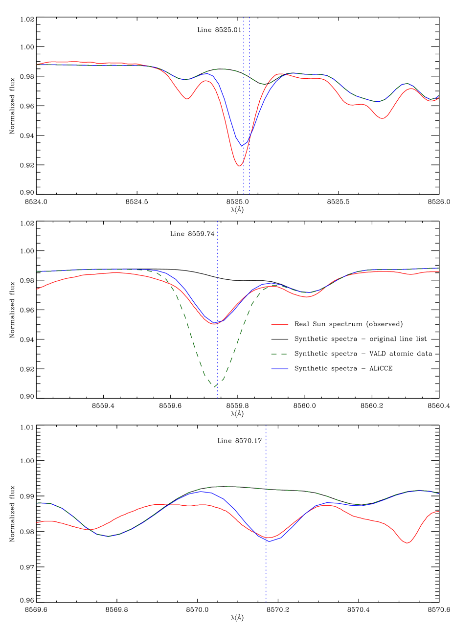
The oscillator strengths could not be derived for five lines given that they did not converge in less than 500 iterations and had errors greater than 0.010 (see details of error evaluation in Martins et al. 2014).
5 Discussion and conclusion
Improving the quality of the synthetic stellar spectra is of paramount importance to our understanding of stars and galaxies. Synthetic spectra libraries has an advantage over empirical spectra ones, which is the possibility of generating spectra with any atmospheric parameters desired for any chemical abundance pattern desired. However, synthetic spectra also have limitations, since they can only be as good as the ingredients used to generate them.
One of the major problems faced by theoretical stellar spectra is the uncertainty and incompleteness of the atomic and molecular line lists used to generate them. There are still many lines present in stellar spectra that are unknown. Moreover, among the millions of known lines present in the line lists, few of them have accurate and precise values, whether they are measured or computed.
We have identified and catalogued missing lines in the atomic and molecular line lists used for producing synthetic stellar spectra in the spectral region of . The line lists that we used are based on previous work by Kurucz (1970); Kurucz & Avrett (1981); Castelli & Kurucz (2004) and updated according to Coelho (2014). For this, we used the observed spectrum of the Sun published by Wallace et al. (2011) and we generated the synthetic spectrum using the spectral synthesis code SYNTHE (Kurucz & Avrett 1981) with the model atmosphere of the Sun generated by ATLAS9 (Kurucz 1970; Sbordone et al. 2004).
We found 39 lines missing from the atomic and molecular line lists within the analysed wavelength region. We performed a characterisation of each line by measuring their equivalent widths and their widths at half maximum (FWHM). From these values and from the analysis of the symmetry of the lines, we conclude that about one-third ( 36%) of the identified lines can be produced or are dominated by a single atomic transition. These are the lines with smaller widths and most symmetric profiles. Wider and asymmetric lines are likely generated by line blends of multiple atomic species or molecules. We searched the identified lines in the NIST atomic database and we found counterparts for 22 of the 39 missing lines, but only 7 had all atomic parameters measured. We added these lines to the atomic list used by the spectral synthesis code, but obtained no improvement in the spectrum produced. This means that the missing lines likely have major contributions of other species.
Because some lines found in NIST lacked the atomic parameters needed to include them in the line list, we also looked for them on VALD. We found counterparts for 14 of these 22 lines, although 8 of them were already included in the line list adopted here. For some of these lines we found more than one counterpart for a given line. All the lines from VALD not present in the atomic line list were from Fe i and Fe ii. Since the atomic parameters from VALD are mostly not produced by measurements in laboratory, but are instead determined empirically or theoretically, we attempted to calibrate the atomic parameters of these lines before including them in the line list.
We used the ALiCCE code (Martins et al. 2014) to calibrate the oscillator strength of the Fe lines missing in the line list. We did not try to calibrate the broadening parameters since the width of the lines is dominated by the rotational velocity of the Sun. The ALiCCE code found better log gf values for 5 of the 10 lines. The new values significantly improved the reproduction of the solar spectrum. For the remaining lines the code has not been able to find results that could improve the reproduction of the solar spectrum.
Acknowledgements.
We would like to thank Robert Kurucz, the referee of this paper, for his valuable comments that definitely improved the paper. We would like to thank Gillian Nave for helping with the search of some of the unidentified lines. J.R.K. acknowledges FAPESP (2014/00502-9) and CAPES for financial support. L.M. thanks CNPQ for financial support through grant 303697/2015-6 and FAPESP through grant 2015/14575-0. P.C. acknowledges CNPQ for financial support through grant 305066/2015-3.References
- Anstee & O’Mara (1995) Anstee, S. D. & O’Mara, B. J. 1995, MNRAS, 276, 859
- Asplund et al. (2005) Asplund, M., Grevesse, N., & Sauval, A. J. 2005, in Astronomical Society of the Pacific Conference Series, Vol. 336, Cosmic Abundances as Records of Stellar Evolution and Nucleosynthesis, ed. T. G. Barnes, III & F. N. Bash, 25
- Asplund et al. (2009) Asplund, M., Grevesse, N., Sauval, A. J., & Scott, P. 2009, ARA&A, 47, 481
- Bacławski (2011) Bacławski, A. 2011, European Physical Journal D, 61, 327
- Barklem et al. (1998) Barklem, P. S., Anstee, S. D., & O’Mara, B. J. 1998, PASA, 15, 336
- Barklem & Aspelund-Johansson (2005) Barklem, P. S. & Aspelund-Johansson, J. 2005, Astron. and Astrophys., 435, 373, (BAJ)
- Barklem & O’Mara (1997) Barklem, P. S. & O’Mara, B. J. 1997, MNRAS, 290, 102
- Barklem et al. (2000) Barklem, P. S., Piskunov, N., & O’Mara, B. J. 2000, A&AS, 142, 467
- Bell et al. (1994) Bell, R. A., Paltoglou, G., & Tripicco, M. J. 1994, MNRAS, 268, 771
- Bertone (2006) Bertone, E. 2006, Mem. S. A. It. Suppl., 8
- Bertone et al. (2008) Bertone, E., Buzzoni, A., Chávez, M., & Rodríguez-Merino, L. H. 2008, A&A, 485, 823
- Blackwell-Whitehead et al. (2008) Blackwell-Whitehead, R. J., Pickering, J. C., Jones, H. R. A., Nilsson, H., & Hartman, H. 2008, Journal of Physics Conference Series, 130, 012002
- Borrero et al. (2003) Borrero, J. M., Bellot Rubio, L. R., Barklem, P. S., & del Toro Iniesta, J. C. 2003, A&A, 404, 749
- Castelli & Kurucz (2004) Castelli, F. & Kurucz, R. L. 2004, ArXiv Astrophysics e-prints [astro-ph/0405087]
- Civiš et al. (2012) Civiš, S., Ferus, M., Kubelík, P., et al. 2012, A&A, 542, A35
- Coelho (2014) Coelho, P. R. T. 2014, MNRAS, 440, 1027
- Corliss & Bozman (1962) Corliss, C. H. & Bozman, W. R. 1962, NBS Monograph, Vol. 53, Experimental transition probabilities for spectral lines of seventy elements; derived from the NBS Tables of spectral-line intensities, ed. Corliss, C. H. & Bozman, W. R. (Washington DC: US Government Printing Office), (CBcor)
- Czekala et al. (2015) Czekala, I., Andrews, S. M., Mandel, K. S., Hogg, D. W., & Green, G. M. 2015, ApJ, 812, 128
- de Boer et al. (2005) de Boer, P. T., Kroese, D. P., Mannor, S., & Rubinstein, R. Y. 2005, Annals of Operatons Research, 134, 19
- Den Hartog et al. (2011) Den Hartog, E. A., Lawler, J. E., Sobeck, J. S., Sneden, C., & Cowan, J. J. 2011, ApJS, 194, 35
- Derouich et al. (2003) Derouich, M., Sahal-Bréchot, S., Barklem, P. S., & O’Mara, B. J. 2003, A&A, 404, 763
- Dimitrijević et al. (2003) Dimitrijević, M. S., Ryabchikova, T., Popović, L. Č., Shulyak, D., & Tsymbal, V. 2003, A&A, 404, 1099
- Doyle et al. (2014) Doyle, A. P., Davies, G. R., Smalley, B., Chaplin, W. J., & Elsworth, Y. 2014, MNRAS, 444, 3592
- Dravins et al. (1998) Dravins, D., Lindegren, L., Madsen, S., & Holmberg, J. 1998, Highlights of Astronomy, 11, 564
- Duquette & Lawler (1982) Duquette, D. W. & Lawler, J. E. 1982, Phys. Rev. A, 26, 330, (DLa)
- Fuhr & Wiese (2006) Fuhr, J. R. & Wiese, W. L. 2006, Journal of Physical and Chemical Reference Data, 35, 1669
- Grevesse & Sauval (1998) Grevesse, N. & Sauval, A. J. 1998, Space Sci. Rev., 85, 161
- Jorissen (2004) Jorissen, A. 2004, Physica Scripta Volume T, 112, 73
- Klose et al. (2002) Klose, J. Z., Fuhr, J. R., & Wiese, W. L. 2002, Journal of Physical and Chemical Reference Data, 31, 217
- Kroese et al. (2006a) Kroese, D. P., Porotsky, S., & Rubinstein, R. Y. 2006a, Methodol. Comput. Appl. Probab., 8, 383
- Kroese et al. (2006b) Kroese, D. P., Porotsky, S., & Rubinstein, R. Y. 2006b, Methodol. Comput. Appl. Probab., 8, 383
- Kurucz (1993) Kurucz, R. 1993, ATLAS9 Stellar Atmosphere Programs and 2 km/s grid. Kurucz CD-ROM No. 13. Cambridge, Mass.: Smithsonian Astrophysical Observatory, 1993., 13
- Kurucz (1970) Kurucz, R. L. 1970, SAO Special Report, 309
- Kurucz (1992) Kurucz, R. L. 1992, Rev. Mexicana Astron. Astrofis., 23
- Kurucz (2005) Kurucz, R. L. 2005, Memorie della Societa Astronomica Italiana Supplementi, 8, 189
- Kurucz (2010) Kurucz, R. L. 2010, Robert L. Kurucz on-line database of observed and predicted atomic transitions
- Kurucz (2011) Kurucz, R. L. 2011, Canadian Journal of Physics, 89, 417
- Kurucz (2013) Kurucz, R. L. 2013, Robert L. Kurucz on-line database of observed and predicted atomic transitions
- Kurucz (2014) Kurucz, R. L. 2014, Robert L. Kurucz on-line database of observed and predicted atomic transitions
- Kurucz & Avrett (1981) Kurucz, R. L. & Avrett, E. H. 1981, SAO Special Report, 391
- Kurucz et al. (1984) Kurucz, R. L., Furenlid, I., Brault, J., & Testerman, L. 1984, Solar flux atlas from 296 to 1300 nm
- Kurucz & Peytremann (1975) Kurucz, R. L. & Peytremann, E. 1975, SAO Special Report, 362, 1, (KP)
- Lesage et al. (1999) Lesage, A., Konjevic, N., & Fuhr, J. R. 1999, in American Institute of Physics Conference Series, Vol. 467, Spectral Line Shapes, ed. R. M. Herman, 27–36
- Lindegren & Perryman (1996) Lindegren, L. & Perryman, M. A. C. 1996, A&AS, 116, 579
- Margolin (2005) Margolin, L. 2005, Annals of Operations Research, 134, 201
- Martin et al. (1988) Martin, G., Fuhr, J., & Wiese, W. 1988, J. Phys. Chem. Ref. Data Suppl., 17
- Martins & Coelho (2007) Martins, L. P. & Coelho, P. 2007, MNRAS, 381, 1329
- Martins et al. (2014) Martins, L. P., Coelho, P., Caproni, A., & Vitoriano, R. 2014, MNRAS, 442, 1294
- Mignard (2005) Mignard, F. 2005, in Astronomical Society of the Pacific Conference Series, Vol. 338, Astrometry in the Age of the Next Generation of Large Telescopes, ed. P. K. Seidelmann & A. K. B. Monet, 15
- Minnaert et al. (1940) Minnaert, M., Houtgast, J., & Mulders, G. F. W. 1940, Photometric atlas of the solar spectrum from [lambda] 3612 to [lambda] 8771 with an appendix from [lambda] 3332 to [lambda] 3637
- Mitchell & Livingston (1991) Mitchell, Jr., W. E. & Livingston, W. C. 1991, ApJ, 372, 336
- Munari et al. (2005) Munari, U., Sordo, R., Castelli, F., & Zwitter, T. 2005, A&A, 442, 1127
- Nave et al. (1994) Nave, G., Johansson, S., Learner, R. C. M., Thorne, A. P., & Brault, J. W. 1994, ApJS, 94, 221
- Paxton et al. (2011) Paxton, B., Bildsten, L., Dotter, A., et al. 2011, ApJS, 192, 3
- Pickering et al. (2011) Pickering, J. C., Blackwell-Whitehead, R., Thorne, A. P., Ruffoni, M., & Holmes, C. E. 2011, Canadian Journal of Physics, 89, 387
- Raassen & Uylings (1998) Raassen, A. J. J. & Uylings, P. H. M. 1998, A&A, 340, 300, (RU)
- Rubinstein (1997) Rubinstein, R. Y. 1997, European Journal of Operational Research, 99, 89
- Rubinstein (1999) Rubinstein, R. Y. 1999, Methodology and Computing in Applied Probability, 2, 127
- Ruffoni et al. (2013) Ruffoni, M. P., Allende Prieto, C., Nave, G., & Pickering, J. C. 2013, ApJ, 779, 17
- Safronova et al. (2010) Safronova, U. I., Safronova, A. S., & Johnson, W. R. 2010, Journal of Physics B Atomic Molecular Physics, 43, 144001
- Sbordone et al. (2004) Sbordone, L., Bonifacio, P., Castelli, F., & Kurucz, R. L. 2004, Memorie della Societa Astronomica Italiana Supplementi, 5, 93
- Shchukina & Vasil’eva (2013) Shchukina, N. G. & Vasil’eva, I. E. 2013, Kinematics and Physics of Celestial Bodies, 29, 53
- Short & Lester (1996) Short, C. I. & Lester, J. B. 1996, ApJ, 469, 898
- Smith (1978) Smith, M. A. 1978, ApJ, 224, 584
- Stalin et al. (1997) Stalin, C. S., Trivedi, C., Sinha, K., & Sanwal, B. B. 1997, Bulletin of the Astronomical Society of India, 25, 353
- Taklif (1990) Taklif, A. G. 1990, Phys. Scr, 42, 69
- Wahlgren (2005) Wahlgren, G. M. 2005, Memorie della Societa Astronomica Italiana Supplementi, 8, 108
- Wallace et al. (2011) Wallace, L., Hinkle, K. H., Livingston, W. C., & Davis, S. P. 2011, ApJS, 195, 6
- Ward et al. (1985) Ward, L., Vogel, O., Arnesen, A., Hallin, R., & Wännström, A. 1985, Phys. Scr, 31, 161, (WV)
- Wiese et al. (2011) Wiese, W. L., Fuhr, J. R., & Bridges, J. M. 2011, in 2010 NASA Laboratory Astrophysics Workshop, C16
- Wiese et al. (1966) Wiese, W. L., Smith, M. W., & Glennon, B. M. 1966, Atomic transition probabilities. Vol.: Hydrogen through Neon. A critical data compilation, ed. Wiese, W. L., Smith, M. W., & Glennon, B. M. (US Government Printing Office), (WSG)
- Wood et al. (2013) Wood, M. P., Lawler, J. E., Sneden, C., & Cowan, J. J. 2013, ApJS, 208, 27