Noise suppression by quantum control before and after the noise

Abstract

We discuss the possibility of protecting the state of a quantum system that goes through noise, by measurements/operations before and after the noise process. The aim is to seek for the optimal protocol that makes the input and output states as close as possible and clarify the role of the measurements therein. We consider two cases; one can perform quantum measurements/operations (i) only after the noise process and (ii) both before and after that. We prove in the two-dimensional Hilbert space that, in the case (i), the noise suppression is essentially impossible for all types of noise and, in the case (ii), the optimal protocol for the depolarizing noise is either the “do nothing” protocol or the “discriminate & reprepare” protocol. These protocols are not “truly quantum” and can be considered as classical. They involve no measurement or only use the measurement outcomes. These results describe the fundamental limitations in quantum mechanics from the viewpoint of control theory. Finally, we conjecture that a statement similar to the case (ii) holds for higher-dimensional Hilbert spaces and present some numerical evidence.

I Introduction

Measurement in quantum theory substantially differs from that in classical theory. One cannot identify the state of a system by measurement on a single sample. In addition, measurement always disturbs the system. The limitation of manipulating quantum systems can be understood as being imposed by these characteristics of quantum measurement. An example is the no-cloning theorem nocloning which states that it is impossible to create identical copies of an arbitrary quantum state. If one could make a clone, then one could extract complete information from a single state by creating infinitely many copies thereof, which contradicts quantum mechanics. Other examples are the facts that one cannot discriminate non-orthogonal states perfectly and that one cannot measure non-commuting observables without errors. In presence of such impossibility, many researchers study how well one can perform these tasks mentioned above. Imperfect cloning buzhil ; werner98 , state discrimination helstrom ; unambig123 and uncertainty relations for noise and disturbance ozawaan ; watanabe are examples of the studies that make a quantitative assessment of ability to realize the tasks approximately.

We would like to discuss an aspect of the limitations of quantum operation that one cannot protect states against noise. Here we use the word “noise” in a wide sense so that it refers to any irreversible dynamics induced by environments. In classical systems, one can protect a state against the irreversible dynamics (noise) if accurate measurements and operations can be done and if the state is not a statistical mixture, by taking the complete record of the state before the noise affects the system. In quantum theory, it is not the case even if the state is pure. Measurement cannot be done accurately and disturbs the state. Nevertheless, one can still consider operations which approximately reverse the noise. Such approximate operations reveal the limit beyond which the noise cannot be suppressed any further. It also is interesting to understand the role which measurement plays for the task.

Noise suppression, the attempt to protect a certain class of states against given noise, is an important problem in the field of quantum control. Many researchers are working on the problem in various ways. Some try to protect a few states, while others try to protect all the pure states. The approaches are further classified by whether one uses ex-post control only or ex-ante and ex-post control together, where we mean by ex-ante and ex-post control the quantum measurements/operations performed before and after, respectively, the noise process. For the problem of protecting two states, Brańczyk et al. bramen07 obtained the optimal ex-post control for the dephasing noise. After a while, Mendonça et al. mengil08 gave a method for constructing the optimal ex-post control for arbitrary noise. Compared to the protection of two states, protecting all the pure states is more difficult and challenging. Zhang et al. zhang08 pointed out a part of the difficulty; they prove that ex-post control alone cannot suppress the depolarizing noise at all. Korotkov and Keane korotkov04 considered ex-ante control as well as ex-post control and found that it is possible to protect, to some extent, all the pure states of a qubit against the amplitude damping noise. Along this line, Wang et al. wang14 made a further study using numerical methods. We remark that there are still many other approaches to reducing the effect of decoherence in a wider context Sho95 ; Kni96 ; Reim05 ; Lid98 ; VioLlo98 .

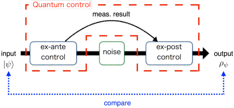
Figure 1: The schematic diagram of the quantum control (ex-ante control and ex-post control).

In this paper, we discuss protection of all the pure states against noise by ex-ante and ex-post control (see Fig. 1). First, we restrict ourselves to the scheme with ex-post control alone and discuss if it can suppress the effect of noise. In the case of the two-dimensional Hilbert space (a qubit), we prove that the suppression is impossible for any type of noise (Theorem 1). This result, generalizing a part of Ref. zhang08 , reveals the decisive necessity of ex-ante control if one wishes to protect all the pure states. Next, we consider the scheme with both ex-ante and ex-post control. We focus on the depolarizing noise, whose isotropic property make the suppression task more difficult, and thus suitable to see the improvement thanks to ex-ante control. Then we show, in Theorem 2, that the optimal control protocols are rather simple and easy to understand classically and ex-ante control is useful only when the noise is strong (Theorem 2). Finally, we conjecture that essentially the same results hold in the case of higher dimensional Hilbert spaces, which is supported by a numerical calculation in the case of three-dimensional Hilbert space.

The paper is organized as follows. In Sec. II, the mathematical tools used in our discussion are reviewed. In Sec. III, the setup of quantum control with ex-ante and ex-post control is explained. In Sec. IV, noise suppression for a qubit by ex-post control alone is discussed in general. We consider in Sec. V ex-ante-ex-post control for a qubit under the depolarizing noise and present a result on the optimal protocols, which is proved in Sec. VI. In Sec. VII, we propose a conjecture for higher-dimensional Hilbert spaces and show some numerical evidence. Sec. VIII is devoted to conclusion and discussions. The Appendix lists the theorems used in the text.

II Basics of quantum operations

In this section, we shall introduce basic mathematical tools and notation used in our analysis. Throughout the paper, we consider physical systems which are represented by a finite-dimensional Hilbert space. Let $\mathcal{H}$ be such a Hilbert space. Let $\mathcal{L(H)}$ be the set of all linear operators on $\mathcal{H}$.

An operator $O\in\mathcal{L(H)}$ is said positive and denoted by $O\geqslant 0$ if $\braket{\psi}{O}{\psi}\geqslant 0$ holds for any $\ket{\psi}\in\mathcal{H}$. A quantum state is described by a density operator $\rho\in\mathcal{L}(\mathcal{H})$ such that $\rho\geqslant 0$ and $\operatorname{Tr}\rho=1$. Fidelity measures closeness of two states and is defined by

$$F(\rho,\ket{\psi}\!\bra{\psi}):=\braket{\psi}{\rho}{\psi}$$ (1)

in the case that at least one of the two states is pure Nielsen . The fidelity represents the probability of measuring $\ket{\psi}$ when the state is $\rho$, and it is equal to unity if and only if $\rho=\ket{\psi}\!\bra{\psi}$.

A linear map $\mathcal{E}:\mathcal{L(H)}\rightarrow\mathcal{L(H)}$ is said positive if $O\geqslant 0$ implies $\mathcal{E}(O)\geqslant 0$. The map $\mathcal{E}$ is said completely positive (CP) if the map $\mathcal{E}\otimes{\mathrm{id}}_{n}$ is positive for every positive integer $n$, where $\mathrm{id}_{n}$ denotes the identity map on $\mathcal{L}(\mathbb{C}^{n})=\mathbb{C}^{n\times n}$. The map $\mathcal{E}$ is said trace-preserving if $\operatorname{Tr}\mathcal{E}(O)=\operatorname{Tr}O$ for any $O\in\mathcal{L(H)}$. A trace-preserving completely positive map is called a TPCP map. It is known that any physical evolution of a quantum state corresponds to a TPCP map, and vice versa Nielsen .

An example of CP map is

$$\mathcal{A}_{A}(O):=AOA^{\dagger}$$ (2)

defined for $A\in\mathcal{L(H)}$. It is known that any CP map can be expressed as a sum of such $\mathcal{A}_{A}$ (the Kraus representation). The CP map $\mathcal{A}_{A}$ is trace-preserving only if $A$ is a unitary operator. Another example of TPCP map, which is important in our discussion below, is mixing with the completely mixed state, or depolarizing noise $\mathcal{D}_{\varepsilon}$, defined by

$$\mathcal{D}_{\varepsilon}(\rho):=(1-\varepsilon)\rho+\varepsilon\frac{1}{d}\operatorname{Tr}\rho,$$ (3)

where $\varepsilon$ is a parameter between 0 and 1, $d$ is the dimensionality of $\mathcal{H}$ and the operator $1/d$ is the completely mixed state. The map outputs the completely mixed state with probability $\varepsilon$ and leaves the input state untouched with probability $1-\varepsilon$.

A family $\{\mathcal{I}_{\omega}\}_{\omega\in\Omega}$ of CP maps with $\sum_{\omega\in\Omega}\mathcal{I}_{\omega}$ being trace-preserving is called a CP instrument. It is known that any physical measuring process corresponds to a CP instrument, and vice versa Ozawa84 . In this paper, we assume that the number of the measurement outcomes is finite. The state evolution by the measurement is described as

$$\rho\mapsto\frac{\mathcal{I}_{\omega}(\rho)}{\operatorname{Tr}\mathcal{I}_{\omega}(\rho)},\quad\text{with probability}\quad\operatorname{Tr}\mathcal{I}_{\omega}(\rho).$$ (4)

A set ${\left\{M_{\omega}\right\}}{}_{\omega\in\Omega}$ of positive operators on $\mathcal{H}$ such that $\sum_{\omega\in\Omega}M_{\omega}=1$ is called a POVM. A CP instrument ${\left\{\operatorname{Tr}\mathcal{I}_{\omega}\right\}}_{\omega\in\Omega}$ defines a POVM by $\operatorname{Tr}\mathcal{I}_{\omega}(\rho)=\operatorname{Tr}\rho M_{\omega}$. We shall say that such a POVM ${\left\{M_{\omega}\right\}}{}_{\omega\in\Omega}$ and a CP instrument ${\left\{\mathcal{I}_{\omega}\right\}}{}_{\omega\in\Omega}$ are associated with each other. A POVM has the information on all statistical properties of the measurement outcomes, while a CP instrument ${\left\{\mathcal{I}_{\omega}\right\}}$ has still more information on the state after the measurement. Any CP instrument associated with ${\left\{M_{\omega}\right\}}{}_{\omega\in\Omega}$ can be written as (See Hayashi Hayashi06 , p.189, Theorem 7.2)

$$\mathcal{I}_{\omega}=\mathcal{K}_{\omega}\circ\mathcal{A}_{\sqrt{M_{\omega}}},$$ (5)

where $\mathcal{K}_{\omega}$ is a TPCP map. We will call ${\left\{\mathcal{A}_{\sqrt{M_{\omega}}}\right\}}_{\omega\in\Omega}$ a simple CP instrument associated with ${\left\{M_{\omega}\right\}}_{\omega\in\Omega}$.

The set $\mathcal{L}(\mathcal{H})$ can be regarded as a Hilbert space with the Hilbert-Schmidt inner product $\braket{X,Y}_{\mathrm{HS}}:=\operatorname{Tr}X^{\dagger}Y$. Then a linear map $\mathcal{E}$ on $\mathcal{L}(\mathcal{H})$ is a linear operator on the Hilbert space $\mathcal{L(H)}$. Thus the trace of $\mathcal{E}\in\mathcal{L}{\left(\mathcal{L}(\mathcal{H})\right)}$ is defined as

$$\operatorname{Tr_{HS}}\mathcal{E}:=\sum_{i}\braket{V_{i},\mathcal{E}(V_{i})}_{\mathrm{HS}},$$ (6)

where $\{V_{i}\}_{i}$ is an orthonormal basis of the Hilbert space $\mathcal{L(H)}$. For example, when $\dim\mathcal{H}=2$, the set of Pauli operators $\{\sigma_{\mu}/\sqrt{2}\}_{\mu=0}^{3}$, with $\sigma_{0}$ being the identity operator, is an orthonormal basis of $\mathcal{L}(\mathcal{H})$ so that the trace of $\mathcal{E}\in\mathcal{L}{\left(\mathcal{L}(\mathcal{H})\right)}$ can be written as

$$\operatorname{Tr_{HS}}\mathcal{E}=\frac{1}{2}\sum_{\mu=0}^{3}\operatorname{Tr}{\left[\sigma_{\mu}\mathcal{E}(\sigma_{\mu})\right]}.$$ (7)

III The setup

In this section, we shall present the main problem and its mathematical formulation.

We consider the ex-ante-ex-post quantum control scheme defined by the following sequence of processes (depicted in Fig. 1):

1. “state preparation”
   An unknown state $\ket{\psi}\in\mathcal{H}$ is prepared.

2. “ex-ante control”
   A measurement is performed, which is described by a CP instrument $\{\mathcal{I}_{\omega}\}_{\omega\in\{1,\dots,M\}}$, where $M$ is a positive integer.

3. “noise”
   The state undergoes an undesired evolution, called “noise,” described by a TPCP map $\mathcal{N}$.

4. “ex-post control”
   An operation, which depends on the measurement outcome $\omega$ of the ex-ante control, is performed on the system. This is described by a family of TPCP maps, $\{\mathcal{C}_{\omega}\}_{\omega\in\{1,\dots,M\}}$, which we call the ex-post control.

For given noise $\mathcal{N}$, an ex-ante-ex-post control protocol is specified by the family $\{(\mathcal{I}_{\omega},\mathcal{C}_{\omega})\}_{\omega\in\{1,\dots,M\}}$. We assume throughout the paper that the prepared state is pure, though one can consider more general mixed state preparation. We also assume that the state $\ket{\psi}$ above is completely unknown, i.e., the probability distribution is uniform on the unit sphere in $\mathcal{H}$.

The problem that we want to consider is, for given noise $\mathcal{N}$, to find an optimal scheme such that the states after the measurement with outcome $\omega$ are as similar to the original state $\ket{\psi}\!\bra{\psi}$ as possible. For defining the optimality, it is natural to introduce some evaluation function $h$ and take an average with respect to the probability of obtaining $\omega$, and then take an average with respect to $\ket{\psi}$ which is completely unknown,

$$\int_{\|\ket{\psi}\|=1}d\psi\sum_{\begin{subarray}{c}\text{measurement}\\ \text{outcomes}\end{subarray}}\text{evaluation function}(\text{final state, initial state})\times\text{ probability}$$

$$= \int_{\|\ket{\psi}\|=1}d\psi\sum_{\omega}h{\left(\mathcal{C}_{\omega}\circ\mathcal{N}{\left(\frac{\mathcal{I}_{\omega}(\ket{\psi}\!\bra{\psi})}{\operatorname{Tr}\mathcal{I}_{\omega}(\ket{\psi}\!\bra{\psi})}\right)},\ket{\psi}\!\bra{\psi}\right)}\operatorname{Tr}\mathcal{I}_{\omega}(\ket{\psi}\!\bra{\psi}),$$ (8)

where the integral is over all unit vectors in $\mathcal{H}$ with the uniform measure normalized by $\int_{\left\|\ket{\psi}\right\|=1}d\psi=1$. We choose the function $h$ to be the fidelity $F$ in Eq. (1). An advantage of the choice is that the resulting total evaluation function, the average fidelity

$$\bar{F}=\int_{\|\ket{\psi}\|=1}d\psi\braket{\psi}{\mathcal{E}(\ket{\psi}\!\bra{\psi})}{\psi},$$ (9)

depends on the protocol ${\left\{(\mathcal{I}_{\omega},\mathcal{C}_{\omega})\right\}}_{\omega}$ only through the average operation

$$\mathcal{E}:=\sum_{\omega=1}^{M}\mathcal{C}_{\omega}\circ\mathcal{N}\circ\mathcal{I}_{\omega}$$ (10)

which is a TPCP map.

We close the section by presenting a useful formula for the average fidelity.

Lemma 1.

The average fidelity $\bar{F}$ is given by

$$\bar{F}=\frac{1}{d(d+1)}\left(d+\operatorname{Tr_{HS}}\mathcal{E}\right),$$ (11)

where $\mathcal{E}$ is the average operation (10) of the protocol ${\left\{(\mathcal{I}_{\omega},\mathcal{C}_{\omega})\right\}}_{\omega}$ and $d:=\dim\mathcal{H}$.

Proof.

Let $S$ be the swap operator, $S(\ket{\psi}\ket{\phi}):=\ket{\phi}\ket{\psi}$, or in an orthonormal basis ${\left\{\ket{ij}\right\}}_{i,j}$, $S=\sum_{ij}\ket{ij}\bra{ji}$. One can easily see that

$$\operatorname{Tr}\left[AB\right]=\operatorname{Tr}\left[S(A\otimes B)\right].$$ (12)

It follows from (9) and (12) that

$$\bar{F}= \operatorname{Tr}\left[S(\mathrm{id}\otimes\mathcal{E})(Q)\right],$$ (13)

where $Q:=\int_{\|\ket{\psi}\|=1}d\psi\ket{\psi}\!\bra{\psi}\otimes\ket{\psi}\!\bra{\psi}$. Then the result is easily obtained by the following formulas,

$$Q=\frac{1+S}{d(d+1)},$$ (14)

$$\operatorname{Tr}\left[S(\mathrm{id}\otimes\mathcal{E})(S)\right]=\operatorname{Tr_{HS}}\mathcal{E}.$$ (15)

Indeed, from (12), (13), (14) and (15), one has

$${\left(d(d+1)\right)}\bar{F} =\operatorname{Tr}\left[S(\mathrm{id}\otimes\mathcal{E})(1)\right]+\operatorname{Tr}\left[S(\mathrm{id}\otimes\mathcal{E})(S)\right]$$

$$=\operatorname{Tr}\mathcal{E}(1)+\operatorname{Tr_{HS}}\mathcal{E}=d+\operatorname{Tr_{HS}}\mathcal{E}.$$ (16)

Let us show (14) and (15). Eq. (14) is seen popescu05 by noting that $Q$ commutes with $U\otimes U$ for any $U$ in $\mathrm{SU}(d)$, the special unitary group on $\mathbb{C}^{d}$. By Schur’s lemma, $Q$ acts as scalar operators on the symmetric and antisymmetric subspaces of $\mathcal{H}\otimes\mathcal{H}$, which are the spaces of irreducible representations. The scalar factors are found easily. Eq. (15) is seen by direct calculation, LHS = $\sum_{ijkl}\bra{ij}{\left(\ket{k}\!\bra{l}\otimes\mathcal{E}{\left(\ket{l}\!\bra{k}\right)}\right)}\ket{ji}=\sum_{ij}\bra{j}\mathcal{E}{\left(\ket{j}\!\bra{i}\right)}\ket{i}$ = RHS. This completes the proof. ∎

IV ex-post control

In this section, we shall consider the noise suppression by ex-post control only (Fig. 2) and present our first main result.

The control sequence has no branches and the protocol is determined by a TPCP map $\mathcal{C}$ describing the ex-post control. Thus our aim is to find the optimal ex-post control $\mathcal{C}$. The average fidelity to be maximized is

$$\bar{F}=\frac{1}{d(d+1)}\left(d+\operatorname{Tr_{HS}}\mathcal{C}\circ\mathcal{N}\right),$$ (17)

from Lemma 1.

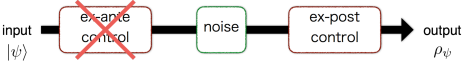
Figure 2: The schematic diagram of the quantum control (only ex-post control).

Theorem 1.

For any noise $\mathcal{N}$ in the two-dimensional Hilbert space $\mathcal{H}$, the optimal ex-post control protocol is a unitary transformation.

Proof.

In the two-dimensional Hilbert space $\mathcal{H}$, we can express a general TPCP map $\mathcal{E}$ in the basis ${\left\{\sigma_{\mu}\right\}}_{0\leqslant\mu\leqslant 3}$ such that

$${\mathcal{E}}(1) =1+\sum_{k=1}^{3}t_{k}\sigma_{k},\quad{\mathcal{E}}(\sigma_{j})=\sum_{j,k=1}^{3}s_{jk}\sigma_{k}.$$ (18)

A necessary condition for positivity and trace-preserving property is $\mathcal{E}(1\pm\sigma_{j})\geqslant 0$, or

$$\sum_{k=1}^{3}|t_{k}\pm s_{jk}|^{2}\leqslant 1.$$ (19)

In the two-dimensional Hilbert space, one can transform the noise $\mathcal{N}$ to $\tilde{\mathcal{N}}$ by unitary operations for the input and output states such that $\tilde{\mathcal{N}}$ has diagonal $s_{jk}$, namely, one has

$$\mathcal{N}=\mathcal{A}_{U}\circ\,\tilde{\mathcal{N}}\circ\mathcal{A}_{V}$$ (20)

with some unitary operators $U$ and $V$ on $\mathcal{H}$, where $\mathcal{A}$ is defined in (2). Introducing $\tilde{\mathcal{C}}:=\mathcal{A}_{V}\circ\,\mathcal{C}\circ\mathcal{A}_{U}$, one has

$$\operatorname{Tr_{HS}}\mathcal{C}\circ\mathcal{N} =\operatorname{Tr_{HS}}\tilde{\mathcal{C}}\circ\tilde{\mathcal{N}}=\frac{1}{2}\sum_{\mu=0}^{3}\operatorname{Tr}\sigma_{\mu}\tilde{\mathcal{C}}\circ\tilde{\mathcal{N}}(\sigma_{\mu})$$

$$=1+\frac{1}{4}\sum_{j=1}^{3}\operatorname{Tr}{\sigma_{j}\tilde{\mathcal{N}}(\sigma_{j})}\,\operatorname{Tr}{\sigma_{j}\tilde{\mathcal{C}}(\sigma_{j})},$$ (21)

where we have used (7) and trace preserving property of $\tilde{\mathcal{C}}$. Because $\tilde{\mathcal{C}}$ is TPCP, (19) implies $\operatorname{Tr}\sigma_{j}\tilde{\mathcal{C}}(\sigma_{j})\leqslant 2$ for $j=1,2,3$, so that

$$\operatorname{Tr_{HS}}\mathcal{C}\circ\mathcal{N}\leqslant 1+\frac{1}{2}\sum_{j=1}^{3}\operatorname{Tr}{\sigma_{j}\tilde{\mathcal{N}}(\sigma_{j})}.$$ (22)

The equality holds only when $\operatorname{Tr}\sigma_{j}\tilde{\mathcal{C}}(\sigma_{j})=2$, so that, by (19) again, one has $\tilde{\mathcal{C}}=\mathrm{id}$. Thus one has $\mathcal{C}=\mathcal{A}_{V}^{-1}\circ\mathcal{A}_{U}^{-1}$, which is a unitary transformation. Then the maximum average fidelity $\bar{F}$ is $(6+\sum_{j}\operatorname{Tr}{\sigma_{j}\tilde{\mathcal{N}}(\sigma_{j})})/12$. ∎

Intuitively, this result says that essentially no ex-post control can suppress the effect of noise if we are completely ignorant of the initial state. On the other hand, when we have some knowledge of the initial state then we can suppress the effect of noise by quantum control bramen07 ; mengil08 . Instead of restricting the candidates for initial state, we consider ex-ante control to extract some information of the initial state, which is discussed in the next section.

From the proof, we find that the quantity $(1/2)\sum_{j}\operatorname{Tr}{\sigma_{j}\tilde{\mathcal{N}}(\sigma_{j})}$ characterizes to what extent the noise is reversible and allows a geometrical interpretation. In the Bloch sphere representation of the state, the whole sphere is mapped to an ellipsoid. Each $(1/2)\operatorname{Tr}{\sigma_{j}\tilde{\mathcal{N}}(\sigma_{j})}$ is the contraction rate along a principal axis.

In closing this section, we remark that an ex-ante-ex-post control with a single branch is equivalent to an ex-post control. In fact, the average fidelity can be written as

$$\bar{F}=\frac{1}{d(d+1)}\Bigl{(}d+\operatorname{Tr_{HS}}\mathcal{I}\circ\mathcal{C}\circ\mathcal{N}\Bigr{)}$$ (23)

by Lemma 1 and the cyclic property of the trace. Here, $\mathcal{I},\mathcal{C}$ are TPCP maps corresponding to ex-ante control and ex-post control, respectively, but the same fidelity can be achieved by an ex-post control $\mathcal{I}\circ\mathcal{C}$.

V ex-ante-ex-post control

In this section, we discuss the noise suppression by ex-ante-ex-post control (Fig. 1) on a qubit. We shall consider the case of two branches because a POVM consisting of two projections gives the optimal discrimination between completely unknown states of a qubit MasPop95 .

In general, there is a trade-off between the information gained and the disturbance caused by the ex-ante control. The ex-ante control can extract some information on the initial state which may be useful for noise suppression. At the same time, the measurement disturbs the state. Thus one might expect that a protocol with a “soft” ex-ante measurement could be optimal. It turns out, however, that this is not the case.

Theorem 2.

Let the noise $\mathcal{N}$ be the depolarizing noise $\mathcal{D}_{\varepsilon}$ defined in (3). For the two-dimensional Hilbert space $\mathcal{H}$, the optimal ex-ante-ex-post control protocol ${\left\{(\mathcal{I}_{\omega},\mathcal{C}_{\omega})\right\}}_{\omega=1,2}$ is given as follows.

(i) When the noise is weak, $\varepsilon\leqslant 2/3$, the “do nothing” protocol is optimal, which is given by

$$\mathcal{I}_{\omega}\propto\mathrm{id},\quad\mathcal{C}_{\omega}=\mathrm{id},\quad\omega=1,2.$$ (24)

The optimal average fidelity is $\bar{F}_{\mathrm{DN}}=1-\varepsilon/2$.

(ii) When the noise is strong, $\varepsilon\geqslant 2/3$, the “discriminate & reprepare” protocol is optimal, which is given by

$$\mathcal{I}_{\omega}(\rho) =\ket{\phi_{\omega}}\!\bra{\phi_{\omega}}\rho\ket{\phi_{\omega}}\!\bra{\phi_{\omega}},$$ (25)

$$\mathcal{C}_{\omega}(\rho) =\ket{\phi_{\omega}}\bra{\phi_{\omega}}{\operatorname{Tr}\rho},$$ (26)

where ${\left\{\ket{\phi_{\omega}}\right\}}_{\omega=1,2}$ is an arbitrary orthonormal basis of $\mathcal{H}$. The optimal average fidelity is $\bar{F}_{\mathrm{DR}}=2/3$.

We give the proof in the next section.

The “do nothing” protocol literally does nothing, and merely lets the system undergo the noise. The value of the average fidelity $\bar{F}_{DN}$ in Theorem 2 can be obtained by direct calculation. Namely, one substitutes $\mathcal{E}=\mathcal{D}_{\varepsilon}$ into the definition (9) of $\bar{F}$ and has

$$\bar{F}_{\textrm{DN}}=\int_{\|\ket{\psi}\|=1}\biggl{(}{(1-\varepsilon)\braket{\psi}{\psi}\!\braket{\psi}{\psi}+\varepsilon\frac{1}{2}\braket{\psi}{\psi}}\biggr{)}=1-\frac{\varepsilon}{2}.$$ (27)

The “discriminate & reprepare” protocol means that one measures and discriminates between a certain two orthogonal states before the noise process and reprepares the corresponding state after the noise process. The value of the average fidelity $\bar{F}_{\mathrm{DR}}$ in Theorem 2 can be calculated as follows. Without loss of generality, one can choose $\ket{\phi_{\omega}}=\ket{\omega}$, $\omega=0,1$, where $\sigma_{3}\ket{0}=\ket{0}$ and $\sigma_{3}\ket{1}=-\ket{1}$. Substituting $\braket{\omega}{\sigma_{3}}{\omega}=(-1)^{\omega}$ and $\braket{\omega}{\sigma_{1}}{\omega}=\braket{\omega}{\sigma_{2}}{\omega}=0$ into (7), one obtains $\operatorname{Tr_{HS}}\mathcal{E}=2$ and hence

$$\bar{F}_{\mathrm{DR}}=\frac{1}{6}\biggl{(}{2+\operatorname{Tr_{HS}}\mathcal{E}}\biggr{)}=\frac{2}{3}$$ (28)

from Lemma 1. It is known from the study of imperfect cloning MasPop95 ; chiribella10 that any “discriminate & reprepare” protocol with arbitrary number of branches does not give a larger value.

If the noise is infinitesimally weak, it is natural that doing nothing is better than the other protocols. If the noise is so strong that the state is completely destroyed after the noise process, one should obtain information on the initial state as much as possible before the system goes through the noise process. The result implies that there is no intermediate regime where the optimal protocol involves weak measurements. The “discriminate & reprepare” protocol only uses the classical information extracted by the ex-ante measurement while the “do nothing” protocol perform no quantum measurement or operation. These protocols are rather classically motivated and are not “truly quantum,” in that they do not reflect any trade-off relation between information gain and disturbance. It is remarkable that these classical control protocols are better than any other quantum control protocols. The result shows that we cannot suppress the noise even if we can perform ex-ante control. This may be understood as fundamental limitations in quantum mechanics.

VI Proof of Theorem 2

In this section, we give a proof of Theorem 2, after showing two lemmas.

Lemma 2.

Let $\mathcal{H}$ be two-dimensional. For any TPCP map $\mathcal{E}$, there exists a TPCP map $\tilde{\mathcal{E}}$ that satisfies

$$\mathcal{D}_{\varepsilon}\circ\mathcal{E}=\tilde{\mathcal{E}}\circ\mathcal{D}_{\varepsilon}.$$ (29)

Proof.

The cases $\varepsilon=0,1$ are trivial so that we assume $\varepsilon\neq 0,1$. Then there exists $\mathcal{D}_{\varepsilon}^{-1}$ which is actually $\mathcal{D}_{-\varepsilon/(1-\varepsilon)}$. One therefore has

$$\tilde{\mathcal{E}}=\mathcal{D}_{\varepsilon}\circ\mathcal{E}\circ\mathcal{D}_{-\varepsilon/(1-\varepsilon)}.$$ (30)

We prove that the map $\tilde{\mathcal{E}}$ is CP, though $\mathcal{D}_{-\varepsilon/(1-\varepsilon)}$ is not. Any Hermiticity-preserving linear map $\sum_{\mu=0}^{3}x^{\mu}\sigma_{\mu}\mapsto\sum_{\mu=0}^{3}x^{\prime}{}^{\mu}\sigma_{\mu}$ is specified by a linear map from $\mathbb{R}^{4}$ to $\mathbb{R}^{4}$, $(x^{\mu})\mapsto(x^{\prime}{}^{\mu})$, $\mu=0,1,2,3$. From a theorem by Ruskai et al. (see the Appendix), the TPCP map $\mathcal{E}$ is expressed as

$$\begin{pmatrix}x^{\prime}{}^{0}\\ \mathbf{x}^{\prime}\end{pmatrix}=\begin{pmatrix}1&0\\ \mathbf{t}&E\end{pmatrix}\begin{pmatrix}x^{0}\\ \mathbf{x}\end{pmatrix},$$ (31)

where $\mathbf{x}=(x^{1},x^{2},x^{3})^{T}$, $\mathbf{t}\in\mathbb{R}^{3}$, $E$ is a $3\times 3$ matrix, and $\mathbf{t}$ and the (signed) singular values $d_{i}$ of $E$ satisfy (65), (67), (68) and (69). In the same way, $\tilde{\mathcal{E}}$ is expressed as

$$\begin{pmatrix}x^{\prime}{}^{0}\\ \mathbf{x}^{\prime}\end{pmatrix}=\begin{pmatrix}1&0\\ (1-\varepsilon)\mathbf{t}&E\end{pmatrix}\begin{pmatrix}x^{0}\\ \mathbf{x}\end{pmatrix}.$$ (32)

Since $0<\varepsilon<1$, the components of the matrix above also satisfy the conditions (65), (67), (68) and (69). Thus $\tilde{\mathcal{E}}$ is TPCP. ∎

Lemma 3.

Let $A$, $\tilde{R}$, $D$ and $R$ be real square matrices. If $A$ and $D$ are diagonal and $\tilde{R}$ is orthogonal, the following inequality holds,

$$\operatorname{Tr}{\left[ARD\tilde{R}\right]}\leqslant\sum_{j}|d_{j}|\biggl{(}{\sum_{i}a_{i}^{2}r_{ij}^{2}}\biggr{)}^{1/2},$$ (33)

where $a_{j}$ and $d_{j}$ are the diagonal elements of $A$ and $D$, respectively, and $r_{ij}$ is the $(i,j)$ element of $R$.

Proof.

Let $\tilde{r}_{ij}$ be the $(i,j)$ element of $\tilde{R}$. One has

$$\operatorname{Tr}{\left[ARD\tilde{R}\right]}=\sum_{ij}a_{i}r_{ij}d_{j}\tilde{r}_{ji}=\sum_{j}|d_{j}|\sum_{i}a_{i}r_{ij}\frac{d_{j}\tilde{r}_{ji}}{|d_{j}|}.$$ (34)

One can view the $i$-sum as an inner product of vectors $(a_{i}r_{ij})_{i}$ and $(d_{j}\tilde{r}_{ji}/|d_{j}|)_{i}$. Applying the Cauchy-Schwarz inequality to the inner product, and using the orthogonality of $\tilde{R}$, one is able to show the claim. ∎

Proof of Theorem 2.

The proof consists of five parts. The main idea is to show that $\bar{F}$ does not exceed the values attained by the “do nothing” and “discriminate & reprepare” protocols.

Step 1. Reduction to simple CP instrument. By Lemma 1, the optimal protocol $\{(\mathcal{I}_{\omega},\mathcal{C}_{\omega})\}_{\omega=1,2}$ is the maximizer of $\sum_{\omega=1}^{2}f_{\omega}$, with

$$f_{\omega}:=\operatorname{Tr_{HS}}\mathcal{C}_{\omega}\circ\mathcal{D}_{\varepsilon}\circ\mathcal{I}_{\omega}.$$ (35)

As was explained in (5), the CP instrument ${\left\{\mathcal{I}_{\omega}\right\}}$ is specified by a family ${\left\{\mathcal{K}_{\omega}\right\}}$ of TPCP maps and a POVM ${\left\{M_{\omega}\right\}}$ so that $\mathcal{I}_{\omega}=\mathcal{K}_{\omega}\circ\mathcal{A}_{\sqrt{M_{\omega}}}$. By Lemma 2, there is a TPCP map $\tilde{\mathcal{K}}_{\omega}$ which satisfies $\mathcal{D}_{\varepsilon}\circ\mathcal{K}_{\omega}=\tilde{\mathcal{K}}_{\omega}\circ\mathcal{D}_{\varepsilon}$. From these, $f_{\omega}$ can be written as

$$f_{\omega} =\operatorname{Tr_{HS}}\mathcal{C}_{\omega}\circ\mathcal{D}_{\varepsilon}\circ\mathcal{K}_{\omega}\circ\mathcal{A}_{\sqrt{M_{\omega}}}$$

$$=\operatorname{Tr_{HS}}\mathcal{C}_{\omega}\circ\tilde{\mathcal{K}}_{\omega}\circ\mathcal{D}_{\varepsilon}\circ\mathcal{A}_{\sqrt{M_{\omega}}}$$

$$=\operatorname{Tr_{HS}}\tilde{\mathcal{C}}_{\omega}\circ\mathcal{D}_{\varepsilon}\circ\mathcal{A}_{\sqrt{M_{\omega}}},$$ (36)

where $\tilde{\mathcal{C}}_{\omega}:=\mathcal{C}_{\omega}\circ\tilde{\mathcal{K}}_{\omega}$. Thus, the original optimization problem for the protocol ${\left\{(\mathcal{C}_{\omega},\mathcal{I}_{\omega})\right\}}$ is translated to that for a protocol $\bigl{\{}{(\tilde{\mathcal{C}}_{\omega},\mathcal{A}_{\sqrt{M_{\omega}}})}\bigr{\}}$ specified by a family of TPCP maps $\bigl{\{}{\tilde{\mathcal{C}}_{\omega}}\bigr{\}}$ and a POVM ${\left\{M_{\omega}\right\}}$.

Let us choose a basis ${\left\{\ket{0},\ket{1}\right\}}$ in which $M_{1}$ and $M_{2}=1-M_{1}$ are diagonal, so that one has

$$M_{\omega}=\alpha_{\omega}\ket{0}\!\bra{0}+\beta_{\omega}\ket{1}\!\bra{1},$$ (37)

$$\alpha_{\omega},\beta_{\omega}\geqslant 0,\quad\sum_{\omega}\alpha_{\omega}=\sum_{\omega}\beta_{\omega}=1.$$ (38)

From (7) and (35), one has $f_{\omega}=\frac{1}{2}{\left(\operatorname{Tr}M_{\omega}+I_{\omega}\right)}$ so that

$$f_{1}+f_{2}=1+\frac{1}{2}(I_{1}+I_{2}),$$ (39)

where

$$I_{\omega}:=\sum_{j=1}^{3}\operatorname{Tr}{\left[\sigma_{j}\tilde{\mathcal{C}}_{\omega}\circ\mathcal{D}_{\varepsilon}\circ\mathcal{A}_{\sqrt{M_{\omega}}}(\sigma_{j})\right]}$$

$$= \,(1-\varepsilon)\sqrt{\alpha_{\omega}\beta_{\omega}}\,\sum_{j=1}^{2}\operatorname{Tr}{\left[\sigma_{j}\tilde{\mathcal{C}}_{\omega}(\sigma_{j})\right]}$$

$$+ \,\frac{\alpha_{\omega}-\beta_{\omega}}{2}\operatorname{Tr}{\left[\sigma_{3}\tilde{\mathcal{C}}_{\omega}(1)\right]}+(1-\varepsilon)\frac{\alpha_{\omega}+\beta_{\omega}}{2}\operatorname{Tr}{\left[\sigma_{3}\tilde{\mathcal{C}}_{\omega}(\sigma_{3})\right]}.$$ (40)

Step 2. Necessity for each $\tilde{\mathcal{C}}_{\omega}$ to be extreme. From here to the end of Step 4, we fix the POVM ${\left\{M_{\omega}\right\}}$ and vary the TPCP maps ${\tilde{\mathcal{C}}_{\omega}}$ to obtain a bound for each $I_{\omega}$. At this stage one can treat each $I_{\omega}$ independently. We drop the subscript $\omega$ from the variables and parameters till Step 4.

Since $f$ is a linear functional of $\tilde{\mathcal{C}}$, we observe that the optimal $\tilde{\mathcal{C}}$ must be one of the extreme points in the convex space of TPCP maps. From a theorem by Ruskai et al. (see the Appendix), such a TPCP map can be written in the form (66) with the condition (70). Thus one has

$$I =(\alpha-\beta)d_{0}r_{33}+(1-\varepsilon)\operatorname{Tr}\left[ARD\tilde{R}\right],$$ (41)

where $R$ and $\tilde{R}$ are real $3\times 3$ rotation matrices, $r_{33}$ is the $(3,3)$ element of $R$, $A:=\operatorname{diag}[2\sqrt{\alpha\beta},2\sqrt{\alpha\beta},\alpha+\beta]$, $D:=\operatorname{diag}[d_{1},d_{2},d_{1}d_{2}]$, $d_{0}^{2}:=(1-d_{1}^{2})(1-d_{2}^{2})$ and $d_{1},d_{2}\in[-1,1]$.

Step 3. An $\tilde{R}$-independent upper bound of $I$. We shall derive an upper bound $J$ of $I$, which is independent from $\tilde{R}$. From Lemma 3, one has

$$\operatorname{Tr}{\left[ARD\tilde{R}\right]}\leqslant\sum_{j}|d_{j}|\biggl{(}{\sum_{i}a_{i}^{2}r_{ij}^{2}}\biggr{)}^{1/2},$$ (42)

where $a_{i}$ and $d_{i}$ are diagonal elements of $A$ and $D$, respectively, and $r_{ij}$ is the $(i,j)$ component of $R$.

Next, it follows from orthogonality of $R$ that the matrix with $(i,j)$ element being $r_{ij}^{2}$ is doubly stochastic. From the Birkhoff-von Neumann theorem (see the Appendix), such a matrix must be a convex combination of permutation matrices. Furthermore, because we are considering the case $a_{1}=a_{2}$ $(=2\sqrt{\alpha\beta})$ in the maximization of $I$, it is enough to consider the case

$$(r_{ij}^{2})_{0\leqslant i,j\leqslant 3}=$$

$$(1-2p){\small\begin{pmatrix}1&&\\ &1&\\ &&1\end{pmatrix}}+(p+q){\small\begin{pmatrix}&&1\\ &1&\\ 1&&\end{pmatrix}}+(p-q){\small\begin{pmatrix}1&&\\ &&1\\ &1&\end{pmatrix}},$$ (43)

where $0\leqslant q\leqslant p\leqslant 1/2$. From (41), (42) and (43), one has

$$I\leqslant J:=\left|(\alpha-\beta)d_{0}\right|\sqrt{1-2p}$$

$$+(1-\varepsilon)\biggl{[}|d_{1}|\sqrt{a_{1}^{2}+(a_{3}^{2}-a_{1}^{2})(p+q)}$$

$$+|d_{2}|\sqrt{a_{1}^{2}+(a_{3}^{2}-a_{1}^{2})(p-q)}+|d_{1}d_{2}|\sqrt{a_{3}^{2}-2(a_{3}^{2}-a_{1}^{2})p}\biggr{]}.$$ (44)

The bound $J$ is a function of $(p,q,d_{1},d_{2})$ while $a_{1}$ and $a_{3}$ are parameters.

Step 4. Joint concavity and a $\tilde{\mathcal{C}}$-independent bound. Let $x:=(d_{1}^{2}+d_{2}^{2})/2$, $y:=(d_{1}^{2}-d_{2}^{2})/2$. Then $J(p,q,x,y)$ is jointly concave with respect to variables $q$ and $y$, which can be easily seen by direct calculation of the Hessian of each term of $J$. Furthermore, $J$ is invariant under $(q,y)\mapsto(-q,-y)$. Thus one has

$$J(p,q,x,y)=\frac{1}{2}\left(J(p,q,x,y)+J(p,-q,x,-y)\right)$$ (45)

$$\leqslant J(p,0,x,0)$$

$$=|\alpha-\beta|(1-x)\sqrt{1-2p}$$

$$\qquad+(1-\varepsilon)\Bigl{[}2\sqrt{x}\sqrt{4\alpha\beta+(\alpha-\beta)^{2}p}$$

$$\qquad\qquad\qquad\qquad+x\sqrt{(\alpha+\beta)^{2}-2(\alpha-\beta)^{2}p}\Bigr{]},$$ (46)

where we have substituted the expressions of $a_{1}$, $a_{2}$ and $d_{0}$. Because $\alpha,\beta\in[0,1]$ and $p\in[0,1/2]$, one can show by a simple observation that the bound (46) does not exceed

$$(1-x)\sqrt{r}+2(1-\varepsilon)\sqrt{x}\sqrt{(\alpha+\beta)^{2}-r}+(1-\varepsilon)(\alpha+\beta)x,$$ (47)

where $r:=(\alpha-\beta)^{2}(1-p)\in[0,1]$. Applying the Cauchy-Schwarz inequality to the first two terms of (47), one sees that (47) does not exceed

$$(\alpha+\beta){\left(\sqrt{(1-x)^{2}+4(1-\varepsilon)^{2}x}+(1-\varepsilon)x\right)}.$$ (48)

This is a convex function of $x$ hence reaches the maximum at the boundary $x=0,1$. Thus, from (44), we arrive at a $\tilde{\mathcal{C}}$-invariant upper bound,

$$I\leqslant(\alpha+\beta)\max{\left\{3(1-\varepsilon),1\right\}}.$$ (49)

Step 5. A protocol-independent bound for $\bar{F}$ and its attainability. We revive the subscript $\omega$. Because $\sum_{\omega}\alpha_{\omega}=\sum_{\omega}\beta_{\omega}=1$, one immediately obtains a protocol-independent upper bound from (49), $I_{1}+I_{2}\leqslant 2\max{\left\{3(1-\varepsilon),1\right\}}$. This is equivalent to

$$\bar{F}\leqslant\frac{1}{6}{\left(3+\max{\left\{3(1-\varepsilon),1\right\}}\right)}.$$ (50)

The values $\bar{F}=1-\varepsilon/2$ and $\bar{F}=2/3$ are attained by “do nothing” and “discriminate & reprepare” protocols, respectively, as was shown in (27) and (28). ∎

VII Higher dimensions

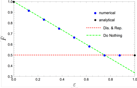
Figure 3: (Color online) The maximum average fidelity $\bar{F}$ achieved by ex-ante-ex-post control for the depolarizing noise of strength $\varepsilon$, when $\dim\mathcal{H}=3$. The (blue) round points are the maxima obtained by numerical optimization, the (black) diamond points are exact values for $\varepsilon=0,1$, the (green) dashed line is $\bar{F}$ achieved by the “do nothing” protocol, and the (red) dotted line is that obtained by the “discriminate & reprepare” protocol. The results support Conjecture 1.

Though Theorem 2 is valid only for the two-dimensional Hilbert space $\mathcal{H}$, similar results may hold in higher dimensions. In this section, we propose a conjecture in general dimensionality and show a numerical evidence for the three-dimensional Hilbert space.

Conjecture 1.

Let $\mathcal{D}_{\varepsilon}$ be the depolarizing noise (3) in the $d$-dimensional Hilbert space $\mathcal{H}$. Then the optimal ex-ante-ex-post control $\{(\mathcal{I}_{\omega},\mathcal{C}_{\omega})\}_{\omega=1}^{d}$ for $\mathcal{D}_{\varepsilon}$ is given as follows.

(i) When the noise is weak, $\varepsilon\leqslant d/(d+1)$, the “do nothing” protocol is optimal, which is given by

$$\mathcal{I}_{\omega}\propto\mathrm{id},\quad\mathcal{C}_{\omega}=\mathrm{id},\quad\omega=1,\dots,d.$$ (51)

The optimal average fidelity is $\bar{F}_{DN}=1-(d-1)\varepsilon/d$.

(ii) When the noise is strong, $\varepsilon\geqslant d/(d+1)$, the “discriminate & reprepare” protocol is optimal, which is given by

$$\mathcal{I}_{\omega}(\rho)= \ket{\phi_{\omega}}\!\bra{\phi_{\omega}}\rho\ket{\phi_{\omega}}\!\bra{\phi_{\omega}},$$ (52)

$$\mathcal{C}_{\omega}(\rho)= \ket{\phi_{\omega}}\!\bra{\phi_{\omega}}\operatorname{Tr}\rho,\quad\quad\quad\quad\quad\omega=1,\dots,d,$$ (53)

where $\{\ket{\phi_{\omega}}\}_{\omega=1}^{d}$ is an arbitrary orthonormal basis of $\mathcal{H}$. The optimal average fidelity is $\bar{F}_{DR}=2/(d+1)$.

The proof of Theorem 2 does not work in the same way because we used a concrete characterization of the extreme points of TPCP maps when $\dim\mathcal{H}=2$.

In our numerical calculation below, we make use of Choi’s correspondence (see the Appendix) which relates the CP maps $\mathcal{C}_{\omega},\mathcal{I}_{\omega}\in\mathcal{L}(\mathcal{L}(\mathcal{H}))$ with positive operators $C_{\omega},I_{\omega}\in\mathcal{L}(\mathcal{H}\otimes\mathcal{H})$, called the Choi operators, as in (63).

Lemma 4.

The average fidelity for an ex-ante-ex-post control protocol ${\left\{(\mathcal{I}_{\omega},\mathcal{C}_{\omega})\right\}}_{\omega=1}^{d}$ is given by

$$\bar{F}= \frac{1}{d(d+1)}\Bigl{(}{d+\sum_{\omega=1}^{d}\operatorname{Tr}{\left[R_{\omega}(\mathrm{id}\otimes\mathcal{N})(S)\right]}}\Bigr{)},$$ (54)

where

$$R_{\omega}:= \operatorname{Tr}_{C}\left[(1_{A}\otimes C_{\omega,CB}^{T})(I_{\omega,AC}\otimes 1_{B})\right],\quad\omega=1,\dots,d,$$ (55)

is the partial transpose of the Choi operator of $\mathcal{I}_{\omega}\circ\mathcal{C}_{\omega}$ [ $\mathcal{H}_{A}$, $\mathcal{H}_{B}$ and $\mathcal{H}_{C}$ are copies of $\mathcal{H}$, $\operatorname{Tr}_{C}$ denotes partial trace on $\mathcal{H}_{C}$, and $X_{AC}$ denotes an operator $X\in\mathcal{L}(\mathcal{H}_{A}\otimes\mathcal{H}_{C})$, etc.].

Proof.

From Lemma 1, it suffices to show

$$\operatorname{Tr_{HS}}\mathcal{C}_{\omega}\circ\mathcal{N}\circ\mathcal{I}_{\omega}=\operatorname{Tr}{\left[R_{\omega}(\mathrm{id}\otimes\mathcal{N})(S)\right]}.$$ (56)

For any linear maps $\mathcal{E}_{1}$ and $\mathcal{E}_{2}$ on $\mathcal{L}(\mathcal{H})$ such that $\mathcal{E}_{1}$ and $\mathcal{E}_{2}^{*}$ commute, one has

$$(\mathcal{E}_{1}\otimes\mathcal{E}_{2})^{*}(S)=(\mathcal{E}_{2}\otimes\mathcal{E}_{1})(S),$$ (57)

where an asterisk denotes the dual linear map. Eq. (57) is seen by (12) because both of $\operatorname{Tr}{\left[(A\otimes B)(\mathcal{E}_{1}\otimes\mathcal{E}_{2})^{*}(S)\right]}$ and $\operatorname{Tr}{\left[(A\otimes B)(\mathcal{E}_{2}\otimes\mathcal{E}_{1})(S)\right]}$ are equal to $\operatorname{Tr}{\left[\mathcal{E}_{1}(A)\mathcal{E}_{2}(B)\right]}$. One has

$$\operatorname{Tr_{HS}}\mathcal{C}_{\omega}\circ\mathcal{N}\circ\mathcal{I}_{\omega}=\operatorname{Tr_{HS}}\mathcal{I}_{\omega}\circ\mathcal{C}_{\omega}\circ\mathcal{N}$$

$$=\operatorname{Tr}{\left[S(\mathrm{id}\otimes(\mathcal{I}_{\omega}\circ\mathcal{C}_{\omega}\circ\mathcal{N}))(S)\right]}$$

$$=\operatorname{Tr}{\left[R_{\omega}(\mathrm{id}\otimes\mathcal{N}))(S)\right]},$$ (58)

where $R_{\omega}=((\mathcal{I}_{\omega}\circ\mathcal{C}_{\omega})\otimes\mathrm{id})(S)$ is the partial transpose on $\mathcal{H}_{B}$ of the Choi operator of $\mathcal{I}_{\omega}\circ\mathcal{C}_{\omega}$ and have used the cyclic property of the trace, (15) and (57). Furthermore, one has

$$R_{\omega} =(\mathcal{I}_{\omega}\otimes\mathrm{id}){\left({\left[(\mathcal{C}_{\omega}\otimes\mathrm{id})(S^{T_{B}})\right]}{}^{T_{B}}\right)}$$

$$=(\mathcal{I}_{\omega}\otimes\mathrm{id})(C_{\omega}{}^{T_{B}})$$

$$=\operatorname{Tr}_{C}{\left[(1_{A}\otimes C_{\omega,CB}{}^{T_{C}T_{B}})(I_{\omega,AC}\otimes\mathrm{id}_{B})\right]},$$ (59)

where $T_{B},T_{C}$ denotes the partial transpose on $\mathcal{H}_{B},\mathcal{H}_{C}$ and we have used the fact that $S^{T_{B}}$ is an unnormalized maximally entangled state $\ket{\Psi}\!\bra{\Psi}$, $\ket{\Psi}=\sum_{i}\ket{ii}$ and (63). ∎

By Lemma 4, the problem of finding optimal $\bar{F}$ and ${\left\{(\mathcal{I}_{\omega},\mathcal{C}_{\omega})\right\}}$ is recast in the following form:

$$\text{maximize}\quad f:=\sum_{\omega=1}^{d}\operatorname{Tr}{\left[R_{\omega}(\mathrm{id}\otimes\mathcal{D}_{\varepsilon})(S)\right]}$$

$$\text{subject to}\quad C_{\omega},I_{\omega}\geqslant 0,\;P=0,$$ (60)

where $R_{\omega}$ is defined in (55) and

$$P:=\sum_{\omega}\operatorname{Tr}\Bigl{[}{\bigl{(}{\operatorname{Tr}_{A}C_{\omega}-1}\bigr{)}^{2}}\Bigr{]}+\operatorname{Tr}\Bigl{[}{\bigl{(}{\operatorname{Tr}_{A}\sum_{\omega}I_{\omega}-1}\bigr{)}^{2}}\Bigr{]}$$ (61)

is the “penalty function.” The conditions $C_{\omega},I_{\omega}\geqslant 0$ imply that complete positivity of $\mathcal{C}_{\omega},\mathcal{I}_{\omega}$ and the condition $P=0$ ensures the trace-preserving property of $\mathcal{C}_{\omega}$ and $\sum_{\omega}\mathcal{I}_{\omega}$ (see the Appendix). When $\varepsilon=0,1$, the problem can be exactly solved for general $d=\dim\mathcal{H}$. For $\varepsilon=0$, the “do nothing” protocol obviously attains the maximum $\bar{F}=1$. For $\varepsilon=1$, it is easy to see that all the protocols fall into “discriminate & reprepare” protocols defined by POVMs. The maximal average fidelity achieved by such protocols is $\bar{F}=2/(d+1)$ chiribella10 .

One can solve the maximization problem (60) in the following steps.

1. Generate $2d$ lower triangular matrices ${\left\{L_{C_{\omega}},L_{I_{\omega}}\right\}}_{1\leqslant\omega\leqslant d}$ so that its nontrivial components are random numbers which obey uniform distribution in the interval $\bigl{[}{-\sqrt{d},\sqrt{d}}\bigr{]}$. The last is a necessary condition for $P=0$.

2. Set the Choi operators as $C_{\omega}=L_{C_{\omega}}L_{C_{\omega}}^{\dagger}$ and $I_{\omega}=L_{I_{\omega}}L_{I_{\omega}}^{\dagger}$. Then $C_{\omega},I_{\omega}\geqslant 0$ automatically hold.

3. Apply a numerical maximization method to $f-\lambda P$, where $\lambda$ is a (large) positive number. The penalty term $-\lambda P$ effectively ensures the condition $P=0$.

We examined Conjecture 1 when $\dim\mathcal{H}=3$. We carried out the numerical scheme above for 5000 initial random points, with $\lambda=10^{3}$ and the maximization method being the simulated annealing. By randomness in the initial data and in the optimization scheme, we expect that the global maximum of $\bar{F}$ are found. Fig. 3 shows the optimal average fidelity $\bar{F}$ as a function of the noise strength $\varepsilon$. The results suggest that either the “do nothing” or “discriminate & reprepare” protocol is optimal, depending on the strength of the noise. This provides evidence for Conjecture 1.

VIII Conclusion and discussions

We have discussed the problem of protecting completely unknown states against given noise by ex-ante and ex-post control scheme. A protocol in the scheme is described mathematically by ${\left\{(\mathcal{I}_{\omega},\mathcal{C}_{\omega})\right\}}_{\omega\in\Omega}$ where ${\left\{\mathcal{I}_{\omega}\right\}}$ is the CP instrument with the set $\Omega$ of outcomes applied before the system goes through the noise and $\mathcal{C}_{\omega}$ are the TPCP maps applied after the system suffered the noise. To evaluate the closeness of the input and output states, we have chosen the average fidelity $\bar{F}$ between the input and output states, which is linear in $\mathcal{I}_{\omega}$ and $\mathcal{C}_{\omega}$. We have shown in Theorem 1 that when the scheme involves ex-post control only, one essentially cannot suppress any given noise. In other words, all one can do is to cancel the unitary rotational part of the noise, if one is completely ignorant of the input state. Next, we have considered ex-ante-ex-post control scheme, focusing on the depolarizing noise. We have shown in Theorem 2 that the optimal average fidelity is achieved by protocols which are not “truly quantum,” or can be understood classically. Namely, if the noise is weak, the “do nothing” protocol is optimal, which does nothing to the system literally, and no other protocol can make a larger average fidelity. If the noise is strong, the “discriminate & reprepare” protocol is optimal. In the protocol, one completely measures the system beforehand, discards the resulting state and reconstructs the state estimated from the measurement. The theorems above are for the two-dimensional Hilbert space. Finally, we have proposed Conjecture 1 that Theorem 2 is essentially true for any dimensionality, or more precisely, the optimal average fidelity is achieved either by the “do nothing” or “discriminate & reprepare” protocol. We have found numerical evidence to support the conjecture in the three-dimensional Hilbert space.

A natural question to ask is whether the result similar to Theorem 2 holds or not for noise other than the depolarizing noise. This is not the case at least for the amplitude damping noise, e.g. spontaneous emission; it is shown numerically that there exists a quantum protocol that can do better than the “do nothing” and “discriminate & reprepare” protocols wang14 . Our result suggests that noise suppression for completely unknown input states is impossible except by using the bias or anisotropy of the noise itself even when one includes the ex-ante control in the scheme. We note that the depolarizing noise is isotropic in the sense that it commutes with arbitrary unitary operations. Thus our result may be understood as describing the fundamental limitations of quantum mechanics from the viewpoint of noise suppression. It is worth pursuing which class of noise allows nontrivial suppression and identifying the optimal controls therein. In particular, it may be important to examine whether Theorem 2 can be extended to all unital noise, the noise that preserves the completely mixed state. Our numerical calculations suggest that it is true at least for the dephasing noise.

Let us discuss our results further in the fundamental aspect: irreversibility of quantum processes. While unitary operations describe reversible processes only, TPCP maps include irreversible processes. Then it is natural to ask to what extent a given TPCP map has irreversibility. For an operator on a Hilbert space, the polar decomposition extracts its “irreversible” part uniquely. However, as far as we know, there is no such a simple and canonical decomposition for TPCP maps, which are operators on Banach spaces. This fact makes it difficult to define the irreversible part of a given TPCP map. In some sense, our work is an attempt to address this problem from the viewpoint of control theory. Using ex-ante and ex-post, we try to cancel an effect of a given TPCP map (noise) and define operationally the irreversible part as what still remains. In Theorem 1, we sought approximate left inverse of a given TPCP map and find it to be a unitary operation. It is not trivial that the approximate left inverse is unique and reversible, which is the conclusion of our theorem. In Theorem 2, using both ex-ante and ex-post control, we found that the irreversible part of the depolarizing noise is itself when the noise is weak.

Appendix A Theorems used in the text

In this Appendix, we shall quote some mathematical facts used in the main text.

A square matrix is said doubly stochastic if all components are nonnegative and if the sum over any row is unity and the sum over any column is unity.

Theorem (Birkoff-von Neumann BvN ).

Any doubly stochastic matrix is a convex combination of permutation matrices.

There is one-to-one correspondence between CP maps and positive operators on a larger Hilbert space.

Theorem (Choi Choi75 ).

Let $\mathcal{H}_{A}$ be a $d$-dimensional Hilbert space and let $\mathcal{H}_{B}$ be a copy of $\mathcal{H}_{A}$. Let $\{\ket{i}\}_{i\in\{1,2,\dots,d\}}$ be an orthonormal basis for each of $\mathcal{H}_{A}$ and $\mathcal{H}_{B}$. Then there is a one-to-one correspondence between a CP map $\mathcal{E}\in\mathcal{L}{\left(\mathcal{L}(\mathcal{H}_{A})\right)}$ and a positive operator $E\in\mathcal{L}{\left(\mathcal{H}_{A}\otimes\mathcal{H}_{B}\right)}$ such that

$$\mathcal{E}(\rho)=\operatorname{Tr}_{B}\left[(1\otimes\rho^{T})E\right],$$ (62)

where $T$ denotes the transpose with respect to the basis above. The operator $E$ is called the Choi operator for $\mathcal{E}$ and is explicitly written as

$$E:=(\mathcal{E}\otimes\mathrm{id}){\left(\ket{\Psi}\!\bra{\Psi}\right)}\in\mathcal{L}(\mathcal{H}_{A}\otimes\mathcal{H}_{B}),$$ (63)

where $\ket{\Psi}:=\sum_{i}\ket{ii}$ is an unnormalized maximally entangled state. The CP map $\mathcal{E}$ is trace-preserving if and only if $\operatorname{Tr}_{A}E=1$.

Let $\mathcal{H}$ be two-dimensional and $\mathcal{E}$ be a Hermiticity-preserving linear map on $\mathcal{L}(\mathcal{H})$. By a parametrization

$$\mathcal{E}\biggl{(}{\sum_{\mu=0}^{3}x^{\mu}\sigma_{\mu}}\biggr{)}=\sum_{\mu=0}^{3}x^{\prime}{}^{\mu}\sigma_{\mu},$$ (64)

$\mathcal{E}$ is expressed as a linear map $\mathbb{R}^{4}\to\mathbb{R}^{4}$, $(x^{\mu})\mapsto(x^{\prime}{}^{\mu})$, ${\mu=0,1,2,3}$. If $\mathcal{E}$ is positive and trace-preserving, then there exist real $3\times 3$ rotation matrices $R,\tilde{R}$ and real numbers $d_{i},t_{i}\;(i=1,2,3)$ such that

$$|t_{i}|+|d_{i}|\leqslant 1,$$ (65)

$$\begin{pmatrix}x^{\prime 0}\\ x^{\prime 1}\\ x^{\prime 2}\\ x^{\prime 3}\\ \end{pmatrix} =\begin{pmatrix}1&0\\ R\begin{pmatrix}t_{1}\\ t_{2}\\ t_{3}\end{pmatrix}&R\begin{pmatrix}d_{1}&&\\ &d_{2}&\\ &&d_{3}\end{pmatrix}\tilde{R}\end{pmatrix}\begin{pmatrix}x^{0}\\ x^{1}\\ x^{2}\\ x^{3}\end{pmatrix}.$$ (66)

Ruskai et al. gave the concrete parametrization of TPCP maps when $\mathcal{H}$ is two-dimensional, extending the work by Fujiwara and Algoet Fuji99 .

Theorem (Ruskai-Szarek-Werner  BethRuskai2002159 , Corollary 2 and Theorem 4).

Let $\mathcal{E}$ a positive, trace-preserving linear map specified by (64), (65) and (66).

(i) The map $\mathcal{E}$ is completely positive if and only if all of the following inequalities hold:

$$(d_{1}+d_{2})^{2}\leqslant(1+d_{3})^{2}-t_{3}^{2}-(t_{1}^{2}+t_{2}^{2})\left(\frac{1+d_{3}\pm t_{3}}{1-d_{3}\pm t_{3}}\right),$$ (67)

$$(d_{1}-d_{2})^{2}\leqslant(1-d_{3})^{2}-t_{3}^{2}-(t_{1}^{2}+t_{2}^{2})\left(\frac{1-d_{3}\pm t_{3}}{1+d_{3}\pm t_{3}}\right),$$ (68)

$$\left[1-(d_{1}^{2}+d_{2}^{2}+d_{3}^{2})-(t_{1}^{2}+t_{2}^{2}+t_{3}^{2})\right]^{2}$$

$$\geqslant 4\left[d_{1}^{2}(t_{1}^{2}+d_{2}^{2})+d_{2}(t_{2}^{2}+d_{3}^{2})+d_{3}^{2}(t_{3}^{2}+d_{1}^{2})-2d_{1}d_{2}d_{3}\right].$$ (69)

(ii) The map $\mathcal{E}$ is in the closure of the set of extreme points of the space of TPCP maps if and only if there exist $R$, $\tilde{R}$ and $d_{1},d_{2}\in[-1,1]$ such that

$$d_{3}=d_{1}d_{2},\quad t_{1}=t_{2}=0,\quad t_{3}^{2}=(1-d_{1}^{2})(1-d_{2}^{2}).$$ (70)

References

- (1) W. K. Wooters, W. H. Zurek, Nature 299, 802 (1982); D. Dieks, Phys. Lett. A 92, 271 (1982); H. P. Yuen, Phys. Lett. A 113, 405 (1986).
- (2) V. Bužek, M. Hillery, Phys. Rev. A 54, 1844 (1996).
- (3) R. F. Werner, Phys. Rev. A 58, 1827 (1998).
- (4) C. W. Helstrom, Inf. Control 10, 254 (1967).
- (5) I. D. Ivanovic, Phys. Lett. A 123, 257 (1987); D. Dieks, Phys. Lett. A 126, 303 (1988); A. Peres, Phys. Lett. A 128, 19 (1988).
- (6) M. Ozawa, Ann. Phys. 311, 350 (2004).
- (7) Y. Watanabe, T. Sagawa, and M. Ueda, Phys. Rev. A 84, 042121 (2011).
- (8) A. M. Brańczyk, P. E. M. F. Mendonça, A. Gilchrist, A. C. Doherty, and S. D. Bartlett, Phys. Rev. A 75, 012329 (2007).
- (9) P. E. M. F. Mendonça, A. Gilchrist, and A. C. Doherty, Phys. Rev. A 78, 012319 (2008).
- (10) S. Zhang, X. Zou, C. Li, C. Jin, and G. Guo, e-print arXiv:0811.3254 (2008).
- (11) A. N. Korotkov and K. Keane, Phys. Rev. A 81, 040103 (2010).
- (12) C. Q. Wang, B. M. Xu, J. Zou, Z. He, Y. Yan, J. G. Li, and B. Shao, Phys. Rev. A 89, 032303 (2014).
- (13) P. W. Shor, Phys. Rev. A 52, R2493 (1995).
- (14) E. Knill and R. Laflamme, Phys. Rev. A 55, 900 (1997).
- (15) M. Reimpell and R. F. Werner, Phys. Rev. Lett. 94 080501 (2005); N. Yamamoto, S. Hara, and K. Tsumura, Phys. Rev. A 71, 022322 (2005).
- (16) D. A. Lidar, I. L. Chuang, and K. B. Whaley, Phys. Rev. Lett. 81, 2594 (1998).
- (17) L. Viola, E. Knill and S. Lloyd, Phys. Rev. Lett. 82, 2417 (1999).
- (18) M. A. Nielsen and I. L. Chuang, Quantum Computation and Quantum Information (Cambridge University Press, Cambridge, 2000).
- (19) M. Ozawa, J. Math. Phys. 25, 79 (1984).
- (20) M. Hayashi, Quantum information: An Introduction (Springer-Verlag, Berlin, 2006).
- (21) S. Popescu, A. J. Short, and A. Winter, e-print arXiv:quant-ph/0511225 (2005).
- (22) S. Massar and S. Popescu, Phys. Rev. Lett. 74, 1259 (1995).
- (23) G. Chiribella, “On quantum estimation, quantum cloning, and finite quantum de Finetti theorems,” Theory of Quantum Computation, Communication, and Cryptography, Lecture Notes in Computer Science, 6519, 9 (2011)
- (24) G. Birkhoff, Univ. Nac. Tucumán Rev. Ser. A 5, 147 (1946); J. von Neumann, Ann. Math. Studies 28, 5 (1953).
- (25) M. D. Choi, Lin. Alg. Appl. 10, 285 (1975).
- (26) A. Fujiwara and P. Algoet, Phys. Rev. A 59, 3290 (1999).
- (27) M. B. Ruskai, S. Szarek, and E. Werner, Lin. Alg. Appl. 347, 159 (2002).