On the solution of linearized (linear in $S$-matrix) Balitsky-Kovchegov equation

Abstract

We revisited solution of a linearized form of leading order Balitsky-Kovchegov equation (linear in $S$-matrix for dipole-nucleus scattering). Here we adopted dipole transverse width dependent cutoff in order to regulate the dipole integral. We also have taken care of all the higher order terms (higher order in the cutoff) that have been reasonably neglected before. The solution reproduces both McLerran-Venugopalan type initial condition (Gaussian in scaling variable) and Levin-Tuchin solution (Gaussian in logarithm of scaling variable) in the appropriate limits. It also connects this two opposite limits smoothly with better accuracy for sets of rescaled rapidity when compared to numerical solutions of full leading order Balitsky-Kovchegov equation.

I Introduction

A typical scattering event in any high energy collider experiment usually involve rapidly growing cascade of gluons. This is partly because high energy (and/or) high virtuality emitted gluons themselves emit further gluons. At high enough energy this cascade of gluons may occupy all the available final state phase space to such an extent that fusion of multiple gluons to single gluon begin to start. This could eventually develop a thermodynamical detail balance with the multiple gluons produced from single gluon which leads to the origin of gluon saturation with a characteristic momentum scale $Q_{s}$ Gribov:1984tu . This is a dynamically generated and energy dependent scale below which stochastic (almost) independent multiple scattering approximations are no longer valid and highly correlated non-linear gluon interactions dominates the phase space. This gluon recombination also restores unitarity of the scattering $S$-matrix which will otherwise violated by an exponential growth of gluon multiplicity. Consequently this saturation of gluons also avoids possible violation of Froissart bound for the total scattering cross section through the power law growth of the Balistky-Fadin-Kuraev-Lipatov (BFKL) bfkl solution which encode energy evolution of the cross-section away from the non-linear region. Unitary corrections to the BFKL equation in the Regge kinematics were first studied by Balitsky Balitsky:1995ub within a Wilson line formalism Balitsky:2001gj and soon after by Kovchegov Kovchegov:1999yj ; Kovchegov:1999ua in the Muller’s color dipole approach Mueller:1993rr ; Mueller:1994jq ; Chen:1995pa . The Balistky hierarchic chain formed by the Wilson line operators reduced to the closed form equation derived by Kovchegov in the large $N_{c}$ limit. Integral kernel in the Balitsky-Kovchegov (BK) equation for both linear and non linear terms are identical and has a simple interpretation of splitting of one parent color dipole into two daughter dipoles. A lot of progress have been made since then in various aspects including solving the equation both analytically and numerically and extending the equation beyond its leading order accuracy Kovchegov:2012mbw . Next to leading order BK equation was derived Balitsky:2008zza , inclusion of running coupling corrections to the BK evolution equations was done Kovchegov:2006vj ; Balitsky:2006wa ; Albacete:2004gw . Solution of the NLO BFKL equation has been found analytically Chirilli:2013kca . Application of the leading order equation extended to jet quenching studies Abir:2015qva . First numerical study for the solution to the NLO Balitsky-Kovchegov equation in coordinate space has been performed recently Lappi:2015fma . Large double logarithms resumed in the QCD evolution of color dipoles Iancu:2015vea and in accordance with the HERA data Iancu:2015joa . An analytic BK solution based on the eigenfunctions of the truncated BFKL equation have been proposed recently that reproduces the initial condition and the high energy asymptotics of the scattering amplitude Bondarenko:2015fca .

In order to have the evolved solution of BK equation one usually starts with the initial condition for the evolution from McLerran-Venugopalan model McLerran:1993ni ; McLerran:1993ka ; McLerran:1994vd or from phenomenological Golec-Biernat and M. Wusthoff model GolecBiernat:1999qd ; GolecBiernat:1998js . The imaginary part of the dipole-nucleus amplitude for deep inelastic scattering of the dipole with a large nucleus takes the following form,

$$N_{\rm MV}(x_{10},Y)=1-S_{MV}(x_{10},Y)=1-\exp\left(-\kappa~{}x_{10}^{2}Q_{s}^{2}(Y)\right)~{},$$ (1)

where $\kappa=1/4$ or could be fixed from the definition of the saturation scale $Q_{s}$ and $x_{10}$ being transverse width of the parent dipole. Eq.(1) is taken as the initial condition for the evolution, and expected to be valid for some initial rapidity both inside and outside the saturation region. The $S$-matrix in Eq.(1) is Gaussian in the scaling variable $\tau$ ($\tau=x_{\perp}Q_{s}(Y)$) with a (model dependent) variance $1/\sqrt{\kappa}$. However in ultra high energy limit where Levin-Tuchin solution Levin:1999mw of Balitsky-Kovchegov equation is valid, $S$-matrix has the following asymptotic expression,

$$N_{\rm LT}(x_{10},Y)=1-S_{\rm LT}(x_{10},Y)=1-\exp\left(-\frac{1+2i\nu_{0}}{4\chi\left(0,\nu_{0}\right)}\ln^{2}\left[x_{10}^{2}Q_{s}^{2}(Y)\right]\right)~{},$$ (2)

Unlike Eq.(1) $S$-matrix in Eq.(2) is a Gaussian in $\ln\tau$ (not in $\tau$). Solution that span over full kinematic range of saturation dynamics is expected to be in accordance with both the McLerran-Venugopalan type initial condition and the Levin-Tuchin solution in their appropriate limits. In this article we have revisited the solution for linearized LO BK equation. By linearized we mean linear in $S$ (unlike BFKL which is linear in $N$) where the term quadratic in $S$ has not been taken. With a modified $x_{\perp}$ dependent form of cutoff in the dipole integral we obtain the general solution as,

$$N(x_{10},Y)=1-S(x_{10},y)=1-\exp\left(\frac{1+2i\nu_{0}}{2\chi\left(0,\nu_{0}\right)}~{}{\rm Li}_{2}\left[-\lambda_{1}x_{10}^{2}Q_{s}^{2}(Y)\right]\right)~{},$$ (3)

where ${\rm Li}_{2}$ is dilogarithm function and $\lambda_{1}(\approx 7.22)$ is a parameter which is be fixed by the definition of $Q_{s}$. Interestingly, Eq.(3) as solution of the linearized BK equation reproduces both Eq.(1) (Gaussian in $\tau=x_{10}Q_{s}(Y)$) and Eq.(2) (Gaussian in logarithm of $\tau=x_{10}Q_{s}(Y)$ $i.e$ in $\ln\tau$) in the limits $\tau=x_{10}Q_{s}(Y)\ll 1$ and $\tau=x_{10}Q_{s}(Y)\gg 1$ respectively. It also connects this two opposite limit smoothly with a better accuracy when compared to numerical solutions of full LO BK equation.

II The dipole integral

One convenient way to address high energy scatterings in QCD is to express the problem in hand in terms of color dipoles degrees of freedom. This approach, originally proposed by Mueller Mueller:1993rr ; Mueller:1994jq ; Chen:1995pa , is formulated in the transverse coordinate space. It has the added advantage that transverse coordinates of the dipoles are not changed during rapidity (or energy) evolution. This makes it easier to include the saturation effects into the model. Typically one starts with a quark (anti-quark) pair in order to calculate probability of emission of a soft gluon off this pair. Both the quark and anti-quark are to follow light cone trajectories and emitted gluons are calculated in the eikonal approximations (the projectile do not suffers any recoil). Adding contributions coming from the quark and anti-quark together with their interference one gluon part of onium wave function found to be proportional to following integral kernel convoluted over the onium wave function with no soft gluon Mueller:1993rr ,

$$I_{\rm dip}\equiv\int d^{2}{x_{2}}~{}\frac{x_{10}^{2}}{x_{20}^{2}x_{21}^{2}}\equiv\int\frac{(x-y)^{2}}{(x-z)^{2}(z-y)^{2}}d^{2}z~{}.$$ (4)

Above kernel (together with a Sudakov type form factor) can be interpreted as emission probability of a soft gluon from the dipole with two pole located at $x$ and $y$. In the large $N_{c}$ limit the emitted gluon can be seen as quark (anti-quark) pair and above formula can be interpreted as probability of decay of original parent dipole at $(x,y)$ of transverse size $x_{10}\equiv|x-y|$ into two new daughter dipoles at $(x,z)$ and at $(z,y)$ with sizes $x_{20}\equiv|x-z|$ and $x_{21}\equiv|z-y|$. In this section we will revisit derivation of above integral which is central to the dipole studies. The integral $I_{\rm dip}$ supplemented with the factor $\bar{\alpha}_{s}/2\pi$ could be interpreted as the differential probability of decay of one parent dipole of transverse size $x_{10}(\equiv x_{1}-x_{0})$ into two daughter dipole of arbitrary sizes. Having note that $d^{2}x_{2}$ is equal to Mueller:1993rr ,

$$2\pi x_{02}x_{12}\int_{0}^{\infty}dkkJ_{0}(kx_{10})J_{0}(kx_{20})J_{0}(kx_{21})dx_{20}dx_{12}$$ (5)

where $J_{0}(z)$ is Bessel function of the first kind, we now write Eq.(4) as Kovchegov:2012mbw ,

$$I_{\rm dip} = 2\pi x_{10}^{2}\int_{0}^{\infty}dkkJ_{0}(kx_{10})\int_{0}^{\infty}\frac{dx_{20}}{x_{20}}J_{0}(kx_{20})\int_{0}^{\infty}\frac{dx_{21}}{x_{21}}J_{0}(kx_{21})~{}.$$ (6)

The integral in Eq.(6) over $x_{20}$ and $x_{21}$ is ill-defined until one specifies a way to regulate the ultra-violate singularities at $x_{20},x_{21}\rightarrow 0$. In the dipole model studies on usually introduce lower cutoff $\rho$ into the $x_{20}$ and $x_{21}$ integrals. This procedure was first adopted by Mueller in Mueller:1993rr and followed in subsequent other studies Kovchegov:1999ua ,

$$\int_{0}^{\infty}\frac{dx}{x}J_{0}(kx)~{}{\Rightarrow}\int_{\rho}^{\infty}\frac{dx}{x}J_{0}(kx)=\ln\frac{2}{k\rho}-\gamma+{\cal O}(\rho)~{}.$$ (7)

Using $\rho$ as a cutoff as usually done in the dipole model studies is one way to regulate the integral. Alternatively, for example, one could replace $1/x^{2}\rightarrow 1/(x^{2}+\rho^{2})$ for $x_{20}^{2}$ and $x_{21}^{2}$ in the denominator in Eq.(6) which gives order zero modified Bessel function of second kind $K_{0}(\rho k)$. There are other ways to regulate the integral. All these regularizations should give the same leading-order result as $\rho\rightarrow 0$, but the sub-leading terms would depend on the regularization procedure that actually been followed. Inside the saturation region $\rho$ usually identified with inverse saturation momentum $1/Q_{s}$. In this study we have revisited this issue with following two points,

(1) We have considered ${\cal O}(\rho)$ and all other higher order terms, in Eq.(7), that have been ignored earlier,

$$\int_{\rho}^{\infty}\frac{dx}{x}J_{0}(kx) = \ln\frac{2}{k\rho}-\gamma+\frac{k^{2}\rho^{2}}{8}~{}{}_{2}F_{3}\left(1,1;~{}2,2,2;~{}-\frac{1}{4}k^{2}\rho^{2}\right)~{},$$ (8)

$$= \ln\frac{2}{k\rho}-\gamma+\sum_{m=1}^{\infty}\frac{(-1)^{m+1}}{2^{2m}(m!)^{2}}\frac{1}{2m}k^{2m}\rho^{2m}~{}.$$

Simple ratio test confirms radius of convergence of this series is infinity. We derived compact closed form expression of $I_{\rm dip}$ that contains contributions from ${\cal O}(\rho)$ and all other higher order terms.

(2) In earlier studies the cutoff $\rho$ usually identified with inverse saturation momentum $1/Q_{s}$ as

$$x_{20},x_{21}\geqslant\rho=\frac{1}{Q_{s}}$$ (9)

or, equivalently,

$$\frac{1}{x_{20}^{2}},\frac{1}{x_{21}^{2}}\leqslant Q_{s}^{2}=\frac{1}{\rho^{2}}$$ (10)

In this study we have adopted similar regularization procedure as done earlier but assumed a general $x_{10}$ dependent form of cutoff as,

$$x_{20},x_{21}\geqslant\rho=\frac{1}{Q_{s}}\frac{1}{\sqrt{\lambda_{1}+\lambda_{2}(1/x_{10}Q_{s})^{2}}}$$ (11)

Eq.(11) actually implies,

$$\frac{1}{x_{20}^{2}},\frac{1}{x_{21}^{2}}\leqslant\lambda_{1}Q_{s}^{2}+\frac{\lambda_{2}}{x_{10}^{2}}=\frac{1}{\rho^{2}}$$ (12)

which can be compared with Eq.(10). Here $\lambda_{1}$ and $\lambda_{2}$ are two positive real parameter which would be fixed in the following way,

(2.a) Parameter $\lambda_{2}$ would be fixed by requiring the fact that in the limit $x_{10}\rightarrow 0$ the dipole integral in Eq.(6) vanishes $i.e.$ $I_{\rm dip}\rightarrow 0$.

(2.b) Parameter $\lambda_{1}$ would be fixed by the definition of saturation momentum : at $x_{10}=1/Q_{s}$, numerical value of $S$-matrix would be half,

$$S\left(x_{10}=1/Q_{s}\right)=\frac{1}{2}~{}.$$ (13)

Eq. (12) is just an ad hoc ansatze for the UV cutoff as the generalization of Eq.(10). However this modified form of cutoff ensures that in both the limit, $Q_{s}\rightarrow\infty~{}(x_{10}~{}{\rm fixed})$ and $x_{10}\rightarrow 0~{}(Q_{s}~{}{\rm fixed})$, the cutoff tends to zero, $\rho\rightarrow 0$. Hence, unlike earlier studies where result is valid only in the limit $Q_{s}\rightarrow\infty$, here the final result is expected to be valid and free from regularization scheme artifacts both in the limit $x_{10}Q_{s}\gg 1$ as well as $x_{10}Q_{s}\ll 1$. With above mentioned modifications $I_{\rm dip}$ found to be, (details are in Appendix I),

$$I_{\rm dip} = 2\pi\ln\left(\lambda_{1}x_{10}^{2}Q_{s}^{2}+\lambda_{2}\right)-2\pi{\rm Li}_{1}\left(\frac{1}{\lambda_{1}x_{10}^{2}Q_{s}^{2}+\lambda_{2}}\right)~{}.$$ (14)

Having note that ${\rm Li}_{1}(z)=-\ln(1-z)$ one may further simplify as,

$$I_{\rm dip} = 2\pi\ln\left(\lambda_{1}x_{10}^{2}Q_{s}^{2}+\lambda_{2}-1\right)~{},$$

$$= 2\pi\ln\left(\lambda_{1}x_{10}^{2}Q_{s}^{2}\right)+2\pi\ln\left(1-\frac{1-\lambda_{2}}{\lambda_{1}x_{10}^{2}Q_{s}^{2}}\right)~{},$$

$$= 2\pi\ln\left(\lambda_{1}x_{10}^{2}Q_{s}^{2}\right)-2\pi{\rm Li}_{1}\left(\frac{1-\lambda_{2}}{\lambda_{1}x_{10}^{2}Q_{s}^{2}}\right)~{}.$$ (16)

Looking at Eq.(II) one could fix $\lambda_{2}$ as $\lambda_{2}=2$ by taking the limit $I_{\rm dip}\rightarrow 0$ when $x_{10}\rightarrow 0$. Therefore, we have,

$$I_{\rm dip} = 2\pi\ln\left(\lambda_{1}x_{10}^{2}Q_{s}^{2}+1\right)~{}.$$ (17)

The parameter $\lambda_{1}$ would be fixed from the definition of $Q_{s}$, in the next section, as mentioned earlier.

III S-Matrix inside saturation region

.

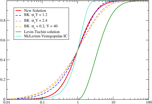
Figure 1: The dipole amplitude $N(x_{10},Y)$ as function of scaling variable $\tau=x_{10}Q_{s}(Y)$; new solution (Eq.(3)) compared with numerical solutions of leading order Balitsky-Kovchegove equation for two sets of rescaled rapidity, $\alpha_{s}Y=1.2,2.4$, one set of fixed coupling $\alpha_{s}=0.2$ for $Y=40$ Albacete:2007yr , McLerran-Venugopalan initial condition Eq.(1) (tweaked to reproduce $N=1/2$ at $\tau=1$) and Levin-Tuchin solution Eq.(2) also displayed for reference.

Scattering $S$-matrix for the color dipole interacting with a large nuclear target can be expressed as expectation value of two light-like path ordered Wilson lines transversely separated by $x_{10}(={\bf x_{\perp}-y_{\perp}})$ as,

$$S(x_{10},Y)=\frac{1}{N_{c}}\langle{\rm Tr}\left[W(x_{\perp},Y)W^{\dagger}(y_{\perp},Y)\right]\rangle~{}.$$ (18)

In large $N_{c}$ limit non-linear energy (or rapidity) evolution of the $S$-matrix is governed by Balitsky-Kovchegov equation,

$$\frac{\partial}{\partial Y}S(x_{01},Y) =\frac{\alpha_{s}N_{c}}{2\pi^{2}}\int d^{2}{x_{2}}~{}\frac{x_{01}^{2}}{x_{02}^{2}x_{21}^{2}}\left[S(x_{02},Y)S(x_{12},Y)-S(x_{01},Y)\right]~{}.$$ (19)

Within the kinematic domain where $S(x_{10})\gg S(x_{02},Y)S(x_{12},Y)$, one can neglect the term quadratic in $S$ in Eq.(19) and the BK equation, an integro-differential equation in general, becomes first order partial differential equation of $S(x_{01},Y)$,

$$\frac{\partial}{\partial Y}S(x_{01},Y) = -\frac{\alpha_{s}N_{c}}{2\pi^{2}}\int d^{2}{x_{2}}~{}\frac{x_{01}^{2}}{x_{02}^{2}x_{21}^{2}}~{}S(x_{01},Y)~{},$$ (20)

In general one expect validity of this linear equation in the limit when $x_{10}>x_{20}$, $x_{21}>1/Q_{s}(Y)$. Here we note that when $x_{20}$, $x_{21}>x_{10}$ we could also expect $S(x_{20})S(x_{21})<S(x_{10})$ $i.e.$ quadratic term is smaller than the linear term in BK equation. Therefore this linearized form should be expected to valid (at least approximately) in both the limiting domain defined by $x_{10}>x_{20},x_{21}$ and $x_{10}<x_{20},x_{21}$. In Eq.(20) the integral over dipole size goes over $x_{02},x_{12}>\rho$ as discussed in the Sec. II with,

$$\rho=\frac{1}{Q_{s}}\frac{1}{\sqrt{\lambda_{1}+2/(Q_{s}^{2}x_{10}^{2})}}~{},$$ (21)

where $\lambda_{2}$ have already been fixed at 2. Using Eq.(16), Eq.(20) can now be written as,

$$\frac{\partial}{\partial Y}\ln S(x_{01},Y) = -\bar{\alpha}_{s}\ln\left[\lambda_{1}x_{10}^{2}Q_{s}^{2}(Y)\right]-\bar{\alpha}_{s}{\rm Li}_{1}\left(-\frac{1}{\lambda_{1}x_{10}^{2}Q_{s}^{2}(Y)}\right)~{}.$$ (22)

Solution of Eq.(22) can be written straightforwardly as,

$$S=S_{0}\exp\left(\frac{1+2i\nu_{0}}{2\chi\left(0,\nu_{0}\right)}\left[\frac{1}{2}\ln^{2}\left(\lambda_{1}x_{10}^{2}Q^{2}_{s}(Y)\right)+{\rm Li}_{2}\left(-\frac{1}{\lambda_{1}x_{10}^{2}Q^{2}_{s}(Y)}\right)\right]\right)~{}.$$ (23)

Here we have used following leading order expression for saturation momentum Gribov:1984tu ,

$$Q_{s}(Y)=Q_{s0}\exp\left(\bar{\alpha}_{s}\frac{\chi\left(0,\nu_{0}\right)}{1+2i\nu_{0}}Y\right)\approx Q_{s0}~{}e^{2.44\bar{\alpha}_{s}Y}$$ (24)

where,

$$\chi(0,\nu)=2\psi(1)-\psi\left(\frac{1}{2}+i\nu\right)-\psi\left(\frac{1}{2}-i\nu\right)$$ (25)

and $\psi$ being digamma function and $S_{0}$ is a constant independent of any initial condition. On can further simplify Eq.(23) to,

$$S=S_{0}\exp\left(\frac{1+2i\nu_{0}}{2\chi\left(0,\nu_{0}\right)}\left[{\rm Li}_{2}\left(-\lambda_{1}x_{10}^{2}Q^{2}_{s}(Y)\right)\right]\right)~{},$$ (26)

where we have used following identity of dilogarithm for $x>0$,

$${\rm Li}_{2}\left(-x\right)+{\rm Li}_{2}\left(-\frac{1}{x}\right)=-\frac{\pi^{2}}{6}-\frac{1}{2}\ln^{2}x~{}.$$ (27)

A factor $\exp\left(\kappa\pi^{2}/6\right)$ with $\kappa=(1+2i\nu_{0})/(2\chi\left(0,\nu_{0}\right))$ has also been absorbed in the normalization constant $S_{0}$. Taking $\chi\left(0,\nu_{0}\right)/(1+2i\nu_{0})\approx 2.44$ from Eq.(24), (initial condition independent) constant $S_{0}$ as unity and defining saturation momentum $Q_{s}$: at $x_{10}=1/Q_{s}$, numerical value of $S$-matrix would be half, $S\left(x_{10}=1/Q_{s}\right)=1/2$, one could now estimate $\lambda_{1}\approx 7.22$. Therefore,

$$S(x_{\perp},Y)=\exp\left(\frac{1+2i\nu_{0}}{2\chi\left(0,\nu_{0}\right)}~{}{\rm Li}_{2}\left[-\lambda_{1}x_{\perp}^{2}Q_{s}^{2}(Y)\right]\right)~{},$$ (28)

with $\lambda_{1}\approx 7.22$. Eq.(28) is main result of this article. Next we have discussed different limits of Eq.(28).

•  In the limit $x_{10}Q_{s}\ll 1/\lambda_{1}\sim 0.14<1$ one may retain only the first term in the dilogarithm series,

$$S(x_{\perp},Y)\approx\exp\left[-1.48~{}x_{10}^{2}Q^{2}_{s}(Y)\right]~{}.$$ (29)

This is Gaussian in the variable $\tau=x_{10}Q_{s}(Y)$ in accordance with McLerran-Venugopalan model McLerran:1993ni ; McLerran:1993ka ; McLerran:1994vd , or Golec-Biernat and M. Wusthoff model GolecBiernat:1999qd ; GolecBiernat:1998js upto a model dependent variance $\sim 1/3$.

• In the black disc limit, $x_{10}Q_{s}\gg\lambda_{1}\sim 7.2>1$, Eq.(26) reproduce Levin-Tuchin solution as,

$$S(x_{\perp},Y)=\exp\left(-\frac{1+2i\nu_{0}}{4\chi\left(0,\nu_{0}\right)}\ln^{2}\left[x_{10}^{2}Q^{2}_{s}(Y)\right]\right)~{},$$ (30)

Here we have used the asymptotic expansion of polylogarithms, ${\rm Li}_{s}\left(z\right)$ in terms of $\ln\left(-z\right)$ and Bernoulli numbers $B_{2k}$ as,

$${\rm Li}_{s}\left(z\right)=\sum_{k=0}^{\infty}(-1)^{k}\left(1-2^{1-2k}\right)(2\pi)^{2k}\frac{B_{2k}}{(2k)!}\frac{\left[\ln(-z)\right]^{s-2k}}{\Gamma\left(s+1-2k\right)}~{}.$$ (31)

In Fig.[1] we have plotted dipole amplitude $N(x_{10},Y)$ as function of scaling variable $\tau=x_{10}Q_{s}(Y)$; new solution (Eq.(3)) compared with numerical solutions of leading order Balitsky-Kovchegove equation for two sets of rescaled rapidity, $\alpha_{s}Y=1.2,2.4$, one set of fixed coupling $\alpha_{s}=0.2$. The solution is in better agreement with the numerical solutions of full LO BK equation in a wide kinematic domain inside saturation region.

IV conclusion and outlook

In this work we have revisited solution of a linearized form of LO BK equation. Unlike the earlier studies here we have adopted transverse width dependent cutoff in order to regulate the dipole integral. We also taken care of all the higher order terms (higher order in cutoff) that have been reasonably neglected before. Later was important in order to make the calculation consistent when away from vanishing cutoff. By demanding that dipole integral vanishes in the limit of vanishing transverse separation of the dipole and defining the inverse of saturation momentum being equal to transverse separation of the parent dipole when dipole amplitude is half we derived a general form of solution which reproduce both McLerran-Venugopalan initial conditions (Gaussian in $\tau$) and Levin-Tuchin solution (Gaussian in $\ln\tau$), with $\tau$ being scaling variable, in their appropriate limits. This new solution involving dilogarithm function connects both this limits smoothly and better approximates the numerical estimation of full leading order Balitsky-Kovchegov equation particularly inside saturation region. This also implies that linearized LO BK equation contains dynamics of dipole nucleus interaction throughout a wide kinematic domain of saturation. It would be interestingly to see how this solution modifies for the running couplings improved or next to leading order BK equations, how it preserves the inherent conformal symmetry of the kernel, or to what extent it receives corrections from quadratic nonlinear term (in $S$-matrix) present in the Balitsky-Kovchegov equation.

Appendix: Calculation of $I_{\rm dip}$

Here we detailed derivation of Eq.(14). Substituting Eq. (8) into Eq. (6) we obtain,

$$I_{\rm dip} = 2\pi x_{10}^{2}\int_{0}^{\infty}dkkJ(x_{10}k)\left(\ln\frac{2}{k\rho}-\gamma_{E}+\sum_{m=1}^{\infty}(-1)^{m+1}{\cal C}_{2m}k^{2m}\rho^{2m}\right)^{2}$$ (32)

$$= I_{0}+I_{1}+I_{2}$$

where,

$$I_{0} = 2\pi x_{10}^{2}\int_{0}^{\infty}dkkJ(x_{10}k)\left(\ln\frac{2}{k\rho}-\gamma_{E}\right)^{2}$$

$$I_{1} = 2\pi x_{10}^{2}\int_{0}^{\infty}dkkJ(x_{10}k)\left(\sum_{m=1}^{\infty}(-1)^{m+1}{\cal C}_{2m}k^{2m}\rho^{2m}\right)^{2}$$

$$I_{2} = 4\pi x_{10}^{2}\int_{0}^{\infty}dkkJ(x_{10}k)\left(\ln\frac{2}{k\rho}-\gamma_{E}\right)\left(\sum_{m=1}^{\infty}(-1)^{m+1}{\cal C}_{2m}k^{2m}\rho^{2m}\right)$$ (33)

with,

$${\cal C}_{2m}=\frac{1}{2m}\frac{1}{2^{2m}(m!)^{2}}$$ (34)

Using,

$$\int_{0}^{\infty}dk~{}k~{}k^{p}~{}J_{0}(x_{10}k)=0$$ (35)

where $x_{10}>0$ and $p$ is either zero or positive even integer,

$$\int_{0}^{\infty}dk~{}k~{}J_{0}(x_{10}k)~{}\ln k=\lim_{\epsilon\rightarrow 0}\frac{\partial}{\partial\epsilon}\int_{0}^{\infty}dk~{}k^{1+\epsilon}~{}J_{0}(x_{10}k)=-\frac{1}{x_{10}^{2}}$$ (36)

and,

$$\int_{0}^{\infty}dk~{}k~{}J_{0}(x_{10}k)~{}\ln^{2}k=\lim_{\epsilon\rightarrow 0}\frac{\partial^{2}}{\partial\epsilon^{2}}\int_{0}^{\infty}dk~{}k^{1+\epsilon}~{}J_{0}(x_{10}k)=\frac{2}{x_{10}^{2}}\left(\ln\frac{x_{10}}{2}+\gamma_{E}\right)$$ (37)

all of which follows from,

$$\int_{0}^{\infty}dkk^{\lambda-1}J_{0}\left(kx\right)=2^{\lambda-1}x^{-\lambda}\frac{\Gamma\left(\lambda/2\right)}{\Gamma\left(1-\frac{\lambda}{2}\right)}~{}.$$ (38)

Using Eq.(36) and Eq.(37) integral $I_{0}$ can be written as,

$$I_{0} = 2\pi x_{10}^{2}\int_{0}^{\infty}dkkJ(x_{10}k)\left(\ln\frac{2}{k\rho}-\gamma_{E}\right)^{2}$$ (39)

$$= 2\pi\ln\left(\frac{x_{10}^{2}}{\rho^{2}}\right)$$

Eq.[35] ensures that $I_{1}$ vanishes for $x_{10}>0$,

$$I_{1} = 2\pi x_{10}^{2}\int_{0}^{\infty}dkkJ(x_{10}k)\left(\sum_{m=1}^{\infty}(-1)^{m+1}{\cal C}_{2m}k^{2m}\rho^{2m}\right)^{2}=0$$ (40)

and terms containing $\gamma_{E}$ and $\ln 2$ in the integral $I_{2}$ in Eq.(33) will vanish as well,

$$I_{2} = 4\pi x_{10}^{2}\int_{0}^{\infty}dkkJ(x_{10}k)\left(\ln\frac{2}{k\rho}-\gamma_{E}\right)\left(\sum_{m=1}^{\infty}(-1)^{m+1}{\cal C}_{2m}k^{2m}\rho^{2m}\right)$$ (41)

$$= -4\pi x_{10}^{2}\sum_{m=1}^{\infty}(-1)^{m+1}{\cal C}_{2m}\int_{0}^{\infty}~{}dk~{}k~{}J(x_{10}k)~{}\ln(k\rho)~{}(k\rho)^{2m}$$

$$= -4\pi x_{10}^{2}\sum_{m=1}^{\infty}(-1)^{m+1}{\cal C}_{2m}\lim_{\epsilon\rightarrow 0}\frac{\partial}{\partial\epsilon}\int_{0}^{\infty}~{}dk~{}k~{}J(x_{10}k)~{}(k\rho)^{2m+\epsilon}~{}.$$

Eq.(38) could be use to evaluate the integral,

$$I_{2} = -4\pi\frac{x_{10}^{2}}{\rho^{2}}\sum_{m=1}^{\infty}(-1)^{m+1}{\cal C}_{2m}\lim_{\epsilon\rightarrow 0}\frac{\partial}{\partial\epsilon}~{}2^{2m+1+\epsilon}~{}\left(\frac{x_{10}}{\rho}\right)^{-2m-2-\epsilon}~{}\frac{\Gamma(m+1+\epsilon/2)}{\Gamma\left(-m-\epsilon/2\right)}$$ (42)

$$= -4\pi\sum_{m=1}^{\infty}(-1)^{m+1}~{}{\cal C}_{2m}~{}2^{2m+1}~{}\left(\frac{\rho}{x_{10}}\right)^{2m}~{}\lim_{\epsilon\rightarrow 0}\frac{\partial}{\partial\epsilon}~{}2^{\epsilon}~{}\left(\frac{x_{10}}{\rho}\right)^{-\epsilon}~{}\frac{\Gamma(1+\epsilon/2)}{\Gamma\left(-\epsilon/2\right)}~{}\prod_{i=1}^{m}\left(i+\frac{\epsilon}{2}\right)^{2}$$

$$= -4\pi\sum_{m=1}^{\infty}(-1)^{m+1}{\cal C}_{2m}2^{2m+1}~{}(-1)^{m}~{}(m!)^{2}~{}\left(\frac{\rho}{x_{10}}\right)^{2m}~{}\left(-\frac{1}{2}\right)$$

$$= -4\pi\sum_{m=1}^{\infty}~{}{\cal C}_{2m}~{}2^{2m}~{}(m!)^{2}~{}\left(\frac{\rho}{x_{10}}\right)^{2m}$$

$$= -2\pi\sum_{m=1}^{\infty}~{}\frac{1}{m}~{}\left(\frac{\rho^{2}}{x_{10}^{2}}\right)^{m}$$

$$= -2\pi~{}{\rm Li}_{1}\left(\frac{\rho^{2}}{x_{10}^{2}}\right)$$

Finally the dipole integral is,

$$I_{\rm dip} = I_{0}+I_{1}+I_{2}$$ (43)

$$= 2\pi\ln\left(\frac{x_{10}^{2}}{\rho^{2}}\right)-2\pi~{}{\rm Li}_{1}\left(\frac{\rho^{2}}{x_{10}^{2}}\right)$$

$$= 2\pi\ln\left(\lambda_{1}x_{10}^{2}Q_{s}^{2}+\lambda_{2}\right)-2\pi{\rm Li}_{1}\left(\frac{1}{\lambda_{1}x_{10}^{2}Q_{s}^{2}+\lambda_{2}}\right)~{},$$

where we have substituted $\rho$ by $Q_{s}$ and $x_{10}$ using Eq.(12) in the last line.

References

• (1) L. V. Gribov, E. M. Levin and M. G. Ryskin, “Semihard Processes in QCD,” Phys. Rept.  100, 1 (1983).
• (2) L. N. Lipatov, Sov. J. Nucl. Phys. 23, (1976) 338; E. A. Kuraev, L. N. Lipatov and V. S. Fadin, Sov. Phys. JETP 45, (1977) 199; I. I. Balitsky and L. N. Lipatov, Sov. J. Nucl. Phys. 28, (1978) 822.
• (3) L. V. Gribov, E. M. Levin and M. G. Ryskin, Phys. Rep. 100 (1983) 1.
• (4) I. Balitsky, “Operator expansion for high-energy scattering,” Nucl. Phys. B 463, 99 (1996) [hep-ph/9509348].
• (5) I. Balitsky, “High-energy QCD and Wilson lines,” In *Shifman, M. (ed.): At the frontier of particle physics, vol. 2* 1237-1342 [hep-ph/0101042].
• (6) Y. V. Kovchegov, “Small x F(2) structure function of a nucleus including multiple pomeron exchanges,” Phys. Rev. D 60, 034008 (1999) [hep-ph/9901281].
• (7) Y. V. Kovchegov, “Unitarization of the BFKL pomeron on a nucleus,” Phys. Rev. D 61, 074018 (2000) [hep-ph/9905214].
• (8) A. H. Mueller, “Soft gluons in the infinite momentum wave function and the BFKL pomeron,” Nucl. Phys. B 415, 373 (1994).
• (9) A. H. Mueller and B. Patel, “Single and double BFKL pomeron exchange and a dipole picture of high-energy hard processes,” Nucl. Phys. B 425, 471 (1994) [hep-ph/9403256].
• (10) Z. Chen and A. H. Mueller, “The Dipole picture of high-energy scattering, the BFKL equation and many gluon compound states,” Nucl. Phys. B 451, 579 (1995).
• (11) Y. V. Kovchegov and E. Levin, “Quantum chromodynamics at high energy,”.
• (12) I. Balitsky and G. A. Chirilli, “Next-to-leading order evolution of color dipoles,” Phys. Rev. D 77, 014019 (2008) [arXiv:0710.4330 [hep-ph]].
• (13) Y. V. Kovchegov and H. Weigert, “Triumvirate of Running Couplings in Small-x Evolution,” Nucl. Phys. A 784, 188 (2007) [hep-ph/0609090].
• (14) I. Balitsky, “Quark contribution to the small-x evolution of color dipole,” Phys. Rev. D 75, 014001 (2007) [hep-ph/0609105].
• (15) J. L. Albacete, N. Armesto, J. G. Milhano, C. A. Salgado and U. A. Wiedemann, “Numerical analysis of the Balitsky-Kovchegov equation with running coupling: Dependence of the saturation scale on nuclear size and rapidity,” Phys. Rev. D 71, 014003 (2005) doi:10.1103/PhysRevD.71.014003 [hep-ph/0408216].
• (16) G. A. Chirilli and Y. V. Kovchegov, “Solution of the NLO BFKL Equation and a Strategy for Solving the All-Order BFKL Equation,” JHEP 1306, 055 (2013) [arXiv:1305.1924 [hep-ph]].
• (17) R. Abir, “Small-$x$ evolution of jet quenching parameter,” Phys. Lett. B 748, 467 (2015) doi:10.1016/j.physletb.2015.07.031 [arXiv:1504.06356 [hep-ph]].
• (18) T. Lappi and H. Mäntysaari, “Direct numerical solution of the coordinate space Balitsky-Kovchegov equation at next to leading order,” Phys. Rev. D 91, no. 7, 074016 (2015) [arXiv:1502.02400 [hep-ph]].
• (19) E. Iancu, J. D. Madrigal, A. H. Mueller, G. Soyez and D. N. Triantafyllopoulos, “Resumming double logarithms in the QCD evolution of color dipoles,” Phys. Lett. B 744, 293 (2015) doi:10.1016/j.physletb.2015.03.068 [arXiv:1502.05642 [hep-ph]].
• (20) E. Iancu, J. D. Madrigal, A. H. Mueller, G. Soyez and D. N. Triantafyllopoulos, “Collinearly-improved BK evolution meets the HERA data,” Phys. Lett. B 750, 643 (2015) doi:10.1016/j.physletb.2015.09.071 [arXiv:1507.03651 [hep-ph]].
• (21) S. Bondarenko and A. Prygarin, “On the Analytic Solution of the Balitsky-Kovchegov Evolution Equation,” JHEP 1506, 090 (2015) doi:10.1007/JHEP06(2015)090 [arXiv:1503.05437 [hep-ph]].
• (22) L. D. McLerran and R. Venugopalan, “Computing quark and gluon distribution functions for very large nuclei,” Phys. Rev. D 49, 2233 (1994) [hep-ph/9309289].
• (23) L. D. McLerran and R. Venugopalan, “Gluon distribution functions for very large nuclei at small transverse momentum,” Phys. Rev. D 49, 3352 (1994) [hep-ph/9311205].
• (24) L. D. McLerran and R. Venugopalan, “Green’s functions in the color field of a large nucleus,” Phys. Rev. D 50, 2225 (1994) [hep-ph/9402335].
• (25) K. J. Golec-Biernat and M. Wusthoff, “Saturation in diffractive deep inelastic scattering,” Phys. Rev. D 60, 114023 (1999) [hep-ph/9903358].
• (26) K. J. Golec-Biernat and M. Wusthoff, “Saturation effects in deep inelastic scattering at low $Q^{2}$ and its implications on diffraction,” Phys. Rev. D 59, 014017 (1998) [hep-ph/9807513].
• (27) E. Levin and K. Tuchin, “Solution to the evolution equation for high parton density QCD,” Nucl. Phys. B 573, 833 (2000) [hep-ph/9908317].
• (28) E. Levin and K. Tuchin, “New scaling at high-energy DIS,” Nucl. Phys. A 691, 779 (2001) [hep-ph/0012167].
• (29) J. L. Albacete and Y. V. Kovchegov, “Solving high energy evolution equation including running coupling corrections,” Phys. Rev. D 75, 125021 (2007) doi:10.1103/PhysRevD.75.125021 [arXiv:0704.0612 [hep-ph]].
• (30) A. Kormilitzin, E. Levin and S. Tapia, “Geometric scaling behavior of the scattering amplitude for DIS with nuclei,” Nucl. Phys. A 872, 245 (2011) [arXiv:1106.3268 [hep-ph]].