Local and global boundary rigidity and the geodesic X-ray transform in the normal gauge

Abstract.

In this paper we analyze the local and global boundary rigidity problem for general Riemannian manifolds with boundary $(M,g)$. We show that the boundary distance function, i.e. $d_{g}|_{\partial M\times\partial M}$, known near a point $p\in\partial M$ at which $\partial M$ is strictly convex, determines $g$ in a suitable neighborhood of $p$ in $M$, up to the natural diffeomorphism invariance of the problem.

We also consider the closely related lens rigidity problem which is a more natural formulation if the boundary distance is not realized by unique minimizing geodesics. The lens relation measures the point and the direction of exit from $M$ of geodesics issued from the boundary and the length of the geodesic. The lens rigidity problem is whether we can determine the metric up to isometry from the lens relation. We solve the lens rigidity problem under the assumption that there is a function on $M$ with suitable convexity properties relative to $g$. This can be considered as a complete solution of a problem formulated first by Herglotz in 1905. We also prove a semi-global results given semi-global data. This shows, for instance, that simply connected manifolds with strictly convex boundaries are lens rigid if the sectional curvature is non-positive or non-negative or if there are no focal points.

The key tool is the analysis of the geodesic X-ray transform on 2-tensors, corresponding to a metric $g$, in the normal gauge, such as normal coordinates relative to a hypersurface, where one also needs to allow weights. This is handled by refining and extending our earlier results in the solenoidal gauge.

1. Introduction and the main result

Boundary rigidity is the question whether the knowledge of the boundary restriction (to $\partial M\times\partial M$) of the distance function $d_{g}$ of a Riemannian metric $g$ on a manifold with boundary $M$ determines $g$, i.e. whether the map $g\mapsto d_{g}|_{\partial M\times\partial M}$ is injective. Apart from its intrinsic geometric interest, this question has major real-life implications, especially if also a stability result and a reconstruction procedure are given. Riemannian metrics in such practical applications represent anisotropic media, for example a sound speed which, relative to the background Euclidean metric, depends on the point, and the direction of propagation. Riemannian metrics in the conformal class of a fixed background metric represent isotropic wave speeds. While many objects of interest are isotropic to a good approximation, this is not always the case: for instance, the inner core of the Earth exhibits anisotropic behavior, see, e.g., [3], as does muscle tissue. The restriction of the distance function to the boundary is then the travel time: the time it takes for waves to travel from one of the points on the boundary to the other. Recall that most of the knowledge of the interior of Earth comes from the study of seismic waves, and in particular travel times of seismic waves; the precise understanding of the boundary rigidity problem is thus very interesting from this perspective as well.

There is a natural diffeomorphism invariance of the boundary rigidity problem: if $\psi$ is a diffeomorphism fixing the boundary pointwise, the boundary distance functions of $g$ and $\psi^{*}g$ are the same. Thus, the precise question is whether $d_{g}|_{\partial M\times\partial M}$ determines $g$ up to this diffeomorphism invariance, i.e. whether there is an isometry $\psi$ (fixing $\partial M$) between $\hat{g}$ and $g$ if the distance functions of $\hat{g}$ and $g$ have the same boundary restriction.

There are counterexamples to this problem, and thus one needs some geometric restrictions. The most common restriction is the simplicity of $(M,g)$: this is the requirement that the boundary is strictly convex and any two points in $M$ can be joined by a unique minimizing geodesic. (Everywhere in this paper, strict convexity means a positive second fundamental form.) Michel [21] conjectured that compact simple manifolds with boundary are boundary rigid. In this paper we prove boundary rigidity or the closely related lens rigidity introduced below in dimensions $n\geq 3$ under a different assumption of the existence of a function with strictly convex level sets. Our assumptions hold for simply connected compact manifolds with strictly convex boundaries such that the geodesic flow has no focal points, or if the sectional curvature is negative (or just non-positive) or if the sectional curvature is non-negative, see Corollary 1.1. In particular, we prove boundary rigidity for simple manifolds in those cases, see Corollary 1.2. This result extends our earlier analogous result which was in a fixed conformal class [34]; recall that the fixed conformal class problem has no diffeomorphism invariance issues to deal with. We prove local (near a boundary point), semiglobal and global rigidity results. The manifolds we study can have conjugate points. Contrary to previous results (except for our conformal result in [34]), we do not assume the metrics to be a priori close before we prove that they are isometric. In that sense, our results are global in the metrics; and also local in the data.

The conformal case has a long history. In 1905 and 1907, Herglotz [9] and Wiechert and Zoeppritz [43] showed that one can recover a radial sound speed $c(r)$ (the metric is $c^{-2}dx^{2}$) in a ball under the condition

(1.1) $$(r/c(r))^{\prime}>0$$

by reducing the problem to solving an Abel type of equation. For simple manifolds, recovery of the conformal factor was proven in [17] and [18], with a stability estimate. We showed in [34] that for $n\geq 3$, one has local and stable recovery near a strictly convex boundary point and semiglobal and global one under the foliation condition we use here, as well. We also showed there that the Herglotz and Wiechert and Zoeppritz condition (1.1) is equivalent to requiring the Euclidean spheres $|x|=\text{const.}$ to be strictly convex in the metric $c^{-2}dx^{2}$.

The first two-dimensional results are for non-positively curved surfaces by Croke [4] and Otal [22]. Boundary rigidity of simple surfaces was proved in [25]. In higher dimensions, simple Riemannian manifolds with boundary are boundary rigid under a priori constant curvature assumptions on the manifold or special symmetries [1], [8]. Several local (in the metric) results near the Euclidean metric are known [32], [7]; in [15] one of the metrics is close to a flat and the other one has an explicit curvature bound; and in [2], one of the metrics is a priori close to the flat one and the other one is arbitrary. The most general result in this direction (outside a fixed conformal class, the setting of [34]) is the generic local (with respect to the metric) one proven in [30], i.e. one is asking whether simple metrics with the same boundary distance function, a priori close to a given one, are isometric; the authors give an affirmative answer in a generic case. Surveys of some of the results can be found in [5, 13, 26, 31].

First we analyze the local boundary rigidity problem for compact Riemannian manifolds $(M,g)$ of dimension $n\geq 3$ with a strictly convex boundary. In fact, compactness is not essential for the local results. More precisely, for suitable relatively open $O\subset M$, including appropriate small neighborhoods of any given point on $\partial M$ or all of $\partial M$ if $\partial M$ is compact, we show that if for two metrics $g_{1},g_{2}$ on $M$, $d_{g_{1}}|_{U\times U}=d_{g_{2}}|_{U\times U}$ for a suitable open set $U$ containing $O\cap\partial M$, then $g_{1}=\psi^{*}g_{2}$ on $O$ for some diffeomorphism $\psi$ fixing $\partial M$ (pointwise, as we understand throughout this paper).

Theorem 1.1.

Suppose that $(M,g)$ is an $n$-dimensional Riemannian manifold with boundary, $n\geq 3$, and assume that $\partial M$ is strictly convex at some $p\in\partial M$ with respect to each of the two metrics $g$ and $\hat{g}$.

(i) If $d_{g}|_{U\times U}=d_{\hat{g}}|_{U\times U}$, for some neighborhood $U$ of $p$ in $\partial M$, then there is a neighborhood $O$ of $p$ in $M$ and a diffeomorphism $\psi:O\to\psi(O)$ fixing $\partial M\cap O$ pointwise such that $g|_{O}=\psi^{*}\hat{g}|_{O}$.

(ii) Furthermore, if the boundary is everywhere strictly convex with respect to each of the two metrics $g$ and $\hat{g}$ and $d_{g}|_{\partial M\times\partial M}=d_{\hat{g}}|_{\partial M\times\partial M}$, then there is a neighborhood $O$ of $\partial M$ in $M$ and a diffeomorphism $\psi:O\to\psi(O)$ fixing $\partial M\cap O$ pointwise such that $g|_{O}=\psi^{*}\hat{g}|_{O}$.

This theorem becomes more precise regarding the open sets discussed above if we consider $M$ (not necessarily compact) as a subset of a manifold without boundary $\tilde{M}$, extend $g$ to $\tilde{M}$; see Figure 1. Our more precise theorem then, to which the above theorem reduces, is the following.

Figure 1. The geometry of the local boundary rigidity problem.

Theorem 1.2.

Suppose that $(M,g)$ is an $n$-dimensional Riemannian manifold with boundary, considered as a domain in $(\tilde{M},g)$, $n\geq 3$, $H$ a hypersurface, and $\tilde{x}$ the signed distance function from $H$, defined near $H$. Suppose that $\{\tilde{x}\geq 0\}\cap M\subset\partial M$, and for some $\delta>0$, $M\cap\{\tilde{x}\geq-\delta\}$ is compact, $\partial M$ is strictly convex in $M\cap\{\tilde{x}>-\delta\}$, the zero level set of $\tilde{x}$ is strictly concave from the superlevel sets in a neighborhood of $M$.

Suppose also that $\hat{g}$ is a Riemannian metric on $M$ with respect to which $\partial M$ is also strictly convex in $M\cap\{\tilde{x}>-\delta\}$.

Then there exists $c_{0}>0$ such that for any $0<c<c_{0}$, with $O=O_{c}=\{\tilde{x}>-c\}\cap M$, if $d_{g}|_{U\times U}=d_{\hat{g}}|_{U\times U}$ for some open set $U$ in $\partial M$ containing $\overline{\{\tilde{x}>-c\}\cap\partial M}$, then there exists a diffeomorphism $\psi:O\to\psi(O)$ fixing $\partial M$ pointwise such that $g|_{O}=\psi^{*}\hat{g}|_{O}$.

Thus, relative to the level sets of $\tilde{x}$, the signed distance function of $H$, we have a very precise statement of where $d_{g}$ and $d_{\hat{g}}$ need to agree on $\partial M$ for us to be able to conclude their equality, up to a diffeomorphism, on $O=O_{c}=\{\tilde{x}>-c\}\cap M$.

We remark that $c$, thus $O$, can be chosen uniformly for a class of $g$ and $\hat{g}$ with uniformly bounded $C^{k}$ norms with some $k$. One can define $C^{k}$ norms of functions and tensor fields by using a fixed finite atlas or by covariant differentiation w.r.t. a fixed metric, as in [15]. From now on, we measure closeness of metrics or boundedness in $C^{k}$, $k\gg 1$.

The slight enlargement, $U$ of $O\cap\partial M$ plays a role because we need to extend $\hat{g}$ to $\tilde{M}$ in a compatible manner, for which we need to recall that if $U$ is an open set in $\partial M$ such that $d_{g}|_{U\times U}=d_{\hat{g}}|_{U\times U}$ then for any compact subset $K$ of $U$ (such as $\overline{O\cap\partial M}$) there is a diffeomorphism $\psi_{0}$ on $M$ such that $\psi_{0}$ is the identity on a neighborhood of $K$ in $\partial M$ and such that $\psi_{0}^{*}\hat{g}$ and $g$ agree to infinite order on a neighborhood of $K$ in $M$ [15, 33]. Replacing $\hat{g}$ by $\psi_{0}^{*}\hat{g}$, then one can extend $\hat{g}$ to $\tilde{M}$ in an identical manner with $g$. In fact, the diffeomorphism $\psi$ is constructed explicitly: it is locally given by geodesic normal coordinates of $\hat{g}$ relative to $H=\{\tilde{x}=0\}$; due to the extension process from $M$ to $\tilde{M}$, $\psi$ is the identity outside $M$. We refer to section 7.1 for more details.

The second problem we study is the lens rigidity one. To define the lens data, we first introduce the manifolds $\partial_{\pm}SM$, defined as the sets of all vectors $(p,v)$ with $p\in\partial M$, $v$ unit in the metric $g$, and pointing outside/inside $M$. We define the scattering relation

$$\mathcal{L}:\partial_{-}SM\longrightarrow\partial_{+}SM$$

in the following way: for each $(p,v)\in\partial_{-}SM$, $\mathcal{L}(p,v)=(q,w)$, where $(q,w)$ are the exit point and direction, if exist, of the maximal unit speed geodesic $\gamma_{p,v}$ in the metric $g$, issued from $(p,v)$. Strict convexity of $\partial M$ is not needed [33] but it is a convenient assumption for a unambiguous definition of $\mathcal{L}$, as a continuous map at least, and we assume it from now on. Let

$$\ell:\partial_{-}SM\longrightarrow\mathbb{R}\cup\infty$$

be its length, possibly infinite. If $\ell<\infty$, we call $M$ non-trapping. The maps $(\mathcal{L},\ell)$ together are called lens relation (or lens data). We identify vectors on $\partial_{\pm}SM$ with their projections on the unit ball bundle $B\partial M$ (each one identifies the other uniquely) and think of $\mathcal{L}$, $\ell$ as defined on the latter with values in itself again, and in $\mathbb{R}\cup\infty$, respectively. With this modification, any diffeomorphism fixing $\partial M$ pointwise does not change the lens relation.

The lens rigidity problem is whether the scattering relation $\mathcal{L}$ (and possibly, $\ell$) determine $(M,g)$ up to an isometry. The lens rigidity problem with partial data is whether we can determine the metric near some $p$ from $\mathcal{L}$ known near the unit sphere $S_{p}\partial M$ considered as a subset of $\partial_{-}SM$, i.e., for vectors with base points close to $p$ and directions pointing into $M$ close to ones tangent to $\partial M$, up to an isometry as above.

Assuming that $\partial M$ is strictly convex at $p\in\partial M$ with respect to $g$, the boundary rigidity and the lens rigidity problems with partial data are equivalent: knowing $d=d_{g}$ near $(p,p)$ is equivalent to knowing $\mathcal{L}$ in some neighborhood of $S_{p}\partial M$. The size of that neighborhood depends on a priori bounds of the derivatives of the metrics with which we work. This equivalence was first noted by Michel [21], since the tangential gradients of $d(p,q)$ on $\partial M\times\partial M$ give us the tangential projections of $-v$ and $w$, see also [33, sec. 3] and [28, sec. 2]. Note that knowledge of $\ell$ may not be needed for the lens rigidity problem (if $\mathcal{L}$ is given only, then the problem is called scattering rigidity in some works) in some situations. For example, for simple manifolds, $\ell$ can be recovered from either $d$ or $\mathcal{L}$; and this includes non-degenerate cases of non-strictly convex boundaries, see for example the proof of [34, Theorem 5.2]; see [42] for a more general result. Also, in [34] it is shown that the lens rigidity problem makes sense even if we do not assume a priori knowledge of $g|_{T\partial M}$.

In fact, that relation of the two rigidity problems is used in our proofs of the first two boundary rigidity theorems. The explicit way we use the equality of $d_{g}|_{U\times U}$ and $d_{\hat{g}}|_{U\times U}$ is via the pseudolinearization formula of Stefanov and Uhlmann [32], see Lemma 7.2, which relies on the equality of the partial lens data.

Vargo [39] proved that non-trapping real-analytic manifolds satisfying an additional mild condition are lens rigid. Croke has shown that if a manifold is lens rigid, a finite quotient of it is also lens rigid [5]. He has also shown that the torus is lens rigid [6]. Stefanov and Uhlmann have shown lens rigidity locally near a generic class of non-simple metrics [33] satisfying an additional microlocal assumption. In a recent work, Guillarmou [11] proved that the lens data determine the conformal class for Riemannian surfaces with hyperbolic trapped sets, no conjugate points and strictly convex boundary, and deformational rigidity in all dimensions under these conditions. The only result we know for the lens rigidity problem with incomplete (but not local) data is for real-analytic metric and metric close to them satisfying the microlocal condition in the next sentence [33]. While in [33], the lens relation is assumed to be known on a subset only, the geodesics issued from that subset cover the whole manifold and their conormal bundle is required to cover $T^{*}M$. In contrast, in this paper, we have localized information.

We then prove the following global consequence of our local results, in which (and also below) we assume that each connected component of $M$ has non-trivial boundary, or, which is equivalent in terms of proving the result, $M$ is connected with non-trivial boundary. As above, we assume $M\subset\tilde{M}$ with some open $\tilde{M}$.

Theorem 1.3.

Assume that $(M,g)$ is a compact $n$-dimensional Riemannian manifold, $n\geq 3$, with strictly convex boundary; $\mathsf{x}$ is a smooth function with non-vanishing differential whose level sets are strictly concave from the superlevel sets; and $\{\mathsf{x}\geq 0\}\cap M\subset\partial M$. Suppose also that $\hat{g}$ is another Riemannian metric on $M$ so that $\partial M$ is strictly convex w.r.t. $\hat{g}$ as well and suppose that the lens relations of $g$ and $\hat{g}$ are the same.

Then there exists a diffeomorphism $\psi:M\to M$ fixing $\partial M$ such that $g=\psi^{*}\hat{g}$.

The assumptions of the theorem are for instance satisfied if $\mathsf{x}$ is the distance function for $g$ from a point outside $M$, near $M$, in $\tilde{M}$, minus the supremum of this distance function on $M$, on a simply connected manifold $\tilde{M}$ and if $(\tilde{M},g)$ has no focal points (near $M$), see Corollary 1.1.

Theorem 1.3 can be viewed as a complete solution of the problem initiated by Herglotz [9] since, as we mentioned above, his condition (1.1) is a foliation condition.

We formulate a semiglobal result as well, whose proof is actually included in the proof of the global Theorem 1.3 below in Section 7. We refer to Figure 2 for an illustration of the theorem.

Theorem 1.4.

Suppose that $M$ is a compact $n$-dimensional Riemannian manifold with a strictly convex boundary, $n\geq 3$. Let $\mathsf{x}$ be a smooth function on $M$ with $[-T,0]$ in its range with $T>0$, $\{\mathsf{x}=0\}\subset\partial M$ and $d\mathsf{x}\not=0$ on $\{-T\leq\mathsf{x}\leq 0\}$. Assume that each hypersurface $\{\mathsf{x}=t\}$, $-T\leq t\leq 0$, is strictly convex and let $M_{0}$ be their union. Let $D\subset\partial_{-}SM$ be a neighborhood of the compact set of all $\beta\in\partial_{-}SM$ which are initial points of geodesics $\gamma_{\beta}$ tangent to the level surfaces of the foliation.

Suppose also that $\hat{g}$ is a Riemannian metric on $M$ with respect to which $\partial M$ is also strictly convex and suppose that the lens relations of $g$ and $\hat{g}$ are the same on $D$. Then there exists a diffeomorphism $\psi:M_{0}\to\psi(M_{0})$ fixing $\partial M$ pointwise such that $g=\psi^{*}\hat{g}$.

The strict convexity of $\partial M$ is used only to show that the jets of $g$ and $\hat{g}$ in boundary normal coordinates coincide. This is true, without convexity, under the mild assumption of no conjugate pairs of points on $\partial M$ [33] which holds automatically for points close enough on a fixed geodesic, which, with a more general definition of the lens relation for non-strictly convex boundaries as in [33] would allow us to remove the strict convexity assumption of $\partial M$ in the theorem but we will not pursue this.

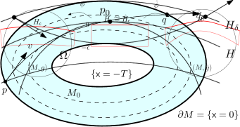
Figure 2. The scattering relation $(p,v)\mapsto(q,w)$ restricted to geodesics in the foliation for the semi-global result.

A special important case arises when there exists a strictly convex function, which may have a critical point $x_{0}$ in $M$ (if so, it is unique). Then we can apply Theorem 1.4 in the exterior of $x_{0}$; which would create a priori a possible singularity of the diffeomorphism at $x_{0}$. In Section 8, we show that this singularity is removable and obtain a global theorem under that assumption, see Theorem 8.1. This condition was extensively studied in [23] (see also the references there). In particular Lemma 2.1 of [23] shows that such a function exists if the sectional curvature of the manifolds is non-negative or if the manifold is simply connected and the curvature is non-positive. Manifolds satisfying one of these conditions are lens rigid:

Corollary 1.1.

Let $(M,g)$ be a compact Riemannian manifold with a strictly convex boundary of dimension $n\geq 3$ satisfying any of the conditions

(a) $(M,g)$ is simply connected with a non-positive sectional curvature;

(b) $(M,g)$ is simply connected and has no focal points;

(c) $(M,g)$ has non-negative sectional curvature.

Then if $g_{1}$ is another metric on $M$ with respect to which $\partial M$ is also strictly convex and with the same lens data, $(M,g)$ is isometric to $(M,g_{1})$ with an isometry fixing the boundary pointwise.

Note that (c) can be replaced by the weaker condition of a lower negative bound of the sectional curvature; depending on some geometric invariants of $(M,g)$, see [23].

As mentioned earlier, the lens rigidity problem and the boundary rigidity problem are equivalent for simple manifolds (which are simply connected). Therefore we have proved Michel’s conjecture in dimension $n\geq 3$ under conditions corresponding to those of Corollary 1.1. More precisely:

Corollary 1.2.

Let $(M,g)$ be a compact simple Riemannian manifold with a strictly convex boundary of dimension $n\geq 3$ satisfying any of the conditions

(a) $(M,g)$ has non-positive sectional curvature;

(b) $(M,g)$ has no focal points;

(c) $(M,g)$ has non-negative sectional curvature.

If $g_{1}$ is another metric on $M$ with respect to which $\partial M$ is also strictly convex and with the same boundary distance function, $(M,g)$ is isometric to $(M,g_{1})$ with an isometry fixing the boundary pointwise. Thus, these classes of Riemannian manifolds are boundary rigid.

Acknowledgments. The authors thank Gabriel Paternain, Mikko Salo and the referees for their valuable suggestions.

2. The approach

This paper relies crucially on the papers [38, 34, 36] both in terms of the approach and in terms of the results; indeed, these three papers can be thought of as being part of a process that culminates with the present result. Thus, we start by discussing these briefly.

The rough picture is that via a linearization procedure, the boundary rigidity problem connects to the geodesic X-ray transform. In the general problem we study here this is the X-ray transform on symmetric 2-tensors explored in [36]. However, in the simpler case of boundary rigidity in a fixed conformal class of metrics, which was proved in [34], it connects to the X-ray transform on functions. The key analytic ideas in the latter setting were introduced in [38]. Relative to [38], the fixed conformal class boundary rigidity problem, [34], required moving to a nonlinear setting. On the other hand, the symmetric 2-tensor X-ray problem is still linear but has a gauge invariance; dealing with this was the key point in [36]. Finally the present paper must combine the ability to deal with the gauge invariance with the ability to work on a non-linear problem. We go through these ingredients one by one.

2.1. The X-ray transform on functions, à la [38]

On a Riemannian manifold $(M,g)$, the geodesic X-ray transform of 2-tensors is a map $C^{\infty}(M)\to C^{\infty}(SM)$

$$If(\beta)=\int_{\gamma_{\beta}}f(\gamma_{\beta}(s))\,ds,$$

where for $\beta\in SM$, $\gamma_{\beta}$ is the lifted geodesic through $\beta$. A key question is if from $If$ we can recover $f$, which can take various forms: injectivity, stability estimates, or perhaps even a construction of a left inverse. Since $I$ is a Fourier integral operator, one general approach is to consider the normal operator, $I^{*}I$. The operator

$$L_{0}v(z)=\int_{S_{z}M}v(\gamma_{z,\zeta})\,d\zeta$$

is actually $I^{*}$ with a suitable natural parameterization of the space of the geodesics [28]

Under the assumption that $M$ has no conjugate points, and working on the extension $\tilde{M}$, $L_{0}I$ is a pseudodifferential operator of order $-1$, and moreover it is elliptic for $n\geq 2$, see [29, 30]. (These requirements can be somewhat relaxed by microlocalization, see [33].) Then there is a parametrix $G$ such that $GL_{0}I$ differs from the identity operator (when restricted to distributions supported in $M$) by a smoothing operator. While this is sufficient for a semi-Fredholm theory, it does not rule out a potentially large finite dimensional nullspace.

The key advance of [38] was to consider a localized problem, which introduced a small parameter, as we now explain. This small parameter is what enables us to rule out the potential large nullspace and thus to construct a left inverse of $L_{0}I$, where $L_{0}$ is a localized version of the $L_{0}$ above. Concretely then, suppose we have a convex foliation, concave from the super-level sets, given by the level sets of a function $\mathsf{x}$ of non-vanishing differential. For a fixed value $\mathsf{c}$ (we use the typeface $\mathsf{c}$ here to distinguish it from the conformal class factor we discuss next), we consider the level set $\mathsf{x}=-\mathsf{c}$ as an artificial boundary, and consider the region $\Omega_{\mathsf{c}}=\{\mathsf{x}>-\mathsf{c}\}\cap M$ for the purpose of finding $f|_{\Omega_{\mathsf{c}}}$ from the information given by the $If(\beta)$ for those $\beta$ for which the geodesic through $\beta$ stays in $\Omega_{\mathsf{c}}$ until it hits $\partial M$, i.e. for $\Omega_{\mathsf{c}}$-localized geodesics. Let $x_{\mathsf{c}}=\mathsf{x}+\mathsf{c}$ be a boundary defining function for $\{\mathsf{x}>-\mathsf{c}\}$ in $\tilde{M}$. In order to implement this analytically, we need to add a cutoff to the definition of $L_{0}$:

$$L_{0}v(z)=\int_{S_{z}M}\chi(z,\zeta)v(\gamma_{z,\zeta})\,d\zeta.$$

Here $\chi$ localizes to a subset of geodesics that are ‘almost tangent’ to level sets of $\mathsf{x}$. The precise type of operator one obtains depends on the precise way one implements the almost tangency. We take this so that on the support of $\chi$, the tangent vector to $\gamma_{z,\zeta}$ at $z$ encloses an angle $\lesssim x_{\mathsf{c}}$ with the level sets of $\mathsf{x}$, i.e. the geodesics become tangent to the level sets as one approaches the artificial boundary at a rate that is roughly proportional to the distance to the artificial boundary. The concavity assumption on the super-level sets implies that these geodesics are indeed $\Omega_{\mathsf{c}}$ local. One could in fact take a somewhat larger angle from tangency just for the concavity considerations, but our choice ensures that $L_{0}I$, or more precisely $e^{-\digamma/x_{\mathsf{c}}}L_{0}Ie^{\digamma/x_{\mathsf{c}}}$, where $\digamma>0$, is a particularly well-behaved elliptic pseudodifferential operator: it is in Melrose’s scattering pseudodifferential algebra which has a powerful symbolic structure and which we discuss in some detail in Section 3. Effectively this means that analytically the artificial boundary acts like a region near infinity in Euclidean space. On the other hand, the parameter $\digamma$ means that we are working on exponentially weight spaces, so the estimates on $f$ (from $If$) will be exponentially weak as one approaches the artificial boundary since $e^{-\digamma/x_{\mathsf{c}}}L_{0}Ie^{\digamma/x_{\mathsf{c}}}$ should be thought of as being applied to $e^{-\digamma/x_{\mathsf{c}}}f$. The key point is that the level set parameter $\mathsf{c}$ becomes a new tool: by taking $\mathsf{c}$ sufficiently small, one can assure that not only is the error of a parametrix ‘smoothing’ (really, ‘Schwartzifying’ in the asymptotically Euclidean interpretation) but is actually small as an operator, so the identity plus this error can be inverted.

Note that the ellipticity now requires $n\geq 3$ because we deal with “almost tangent” (to the actual or to the artificial boundary) geodesics only. If $n=2$, we get ellipticity on codirections close to normal ones only.

In order to invert the X-ray transform globally then one has a layer stripping procedure, in which first one recovers $f$ in $\mathsf{x}\geq-\mathsf{c}_{1}$, $\mathsf{c}_{1}>0$ small, then in $-\mathsf{c}_{1}\geq\mathsf{x}\geq-\mathsf{c}_{2}$, $\mathsf{c}_{2}-\mathsf{c}_{1}>0$ small, etc. Since we can control the step size, compactness considerations result in global injectivity, stability, etc.

2.2. Boundary rigidity in a fixed conformal class, à la [34]

If we have a fixed conformal class, i.e. we study multiples $c^{-2}g_{0}$ of a background metric $g_{0}$, then the linearization (in $c$) of the boundary distance function around a certain $c_{0}$ is an X-ray transform of $\delta c$.

As mentioned already in the introduction, we actually use the lens information. This gives rise to a formula, called the pseudolinearization formula in [32], for the difference of the cotangent bundle coordinates of the point $\tilde{Z}(t,z)$, resp. $Z(t,z)$, of the time $t$ Hamilton flows emanating from a boundary point in the same direction, i.e. from $z=(x,\xi)$, $\xi=g_{x}(\zeta)$:

(2.1) $$\tilde{Z}(t,z)-Z(t,z)=\int_{0}^{t}\frac{\partial\tilde{Z}}{\partial z}(t-s,Z(s,z))\big{(}\tilde{V}-V\big{)}(Z(s,z))\,ds;$$

here $\tilde{V}$ and $V$ are the Hamilton vector fields given by $\tilde{c}^{-2}g_{0}$ and $c^{-2}g_{0}$. If the lens relations are the same, then taking $t$ as the time $\tau(x,\xi)$ at which the respective flows both reach the boundary at the same point, the left hand side vanishes. Expressing the Hamilton vector field in terms of the factors $\tilde{c},c$ and their first derivatives, and taking the momentum (i.e. $\xi$) component of $Z$, we obtain a formula for the integral of the first derivatives of $\tilde{c}-c$ and $\tilde{c}-c$ itself. Since (2.1) integrates the difference of the Hamilton vector fields along the trajectory $Z(.,z)=Z(.,x,\xi)$, i.e. along a bicharacteristic, i.e. a lifted geodesic, this turns to be an X-ray transform with a weight (essentially given by the prefactor in (2.1)). Namely if we write $f=c^{2}-\tilde{c}^{2}$, we obtain

(2.2) $$J_{i}f(\gamma):=\int\left(A_{i}^{j}(X(t),\Xi(t))(\partial_{x^{j}}f)(X(t))+B_{i}(X(t),\Xi(t))f(X(t))\right)\,dt=0,\ \qquad i=1,\ldots,n,$$

for any bicharacteristic $\gamma=(X(t),\Xi(t))$ (related to the speed $c$) in our set $\Omega_{\mathsf{c}}$, where

$$A_{i}^{j}\left(x,\xi\right)= -\frac{1}{2}\frac{\partial\tilde{\Xi}_{i}}{\partial\xi_{j}}(\tau(x,\xi),(x,\xi))c^{-2}(x),$$

$$B_{i}\left(x,\xi\right)= \frac{\partial\tilde{\Xi}_{i}}{\partial x^{j}}(\tau(x,\xi),(x,\xi))g_{0}^{ik}(x)\xi_{k}-\frac{1}{2}\frac{\partial\tilde{\Xi}_{i}}{\partial\xi_{j}}(\tau(x,\xi),(x,\xi))(\partial_{x^{j}}g_{0}^{-1}(x))\xi\cdot\xi.$$

This way, we deal with the geometry of a single metric directly, and the geometry of the other one affects the weight. At the boundary of $M$ we have $A_{i}^{j}(x,\xi)=-\frac{1}{2}c^{-2}\delta_{i}^{j}$. Then the transform given by just the $A_{i}^{j}$ term gives rise to an elliptic pseudodifferential operator by taking $L_{0}$ essentially as above (since we have $n$ components corresponding to the $n$ derivatives, really the $n$ by $n$ matrix version, $L_{0}\operatorname{Id}_{n}$), while the $B_{i}$ terms can be absorbed using a Poincaré-type inequality at least for sufficiently small domains (the foliation parameter is near $0$). This shows that if $Jf$ vanishes then so does $f$, i.e. $c=\tilde{c}$, proving the local version of the boundary rigidity in a fixed conformal class.

2.3. The X-ray transform on tensors, à la [36]

The geodesic X-ray transform of 2-tensors along the geodesics of a metric $g$ is a map $C^{\infty}(M;\mathrm{Sym}^{2}T^{*}M)\to C^{\infty}(SM)$

$$If(\beta)=\int_{\gamma_{\beta}}f(\gamma_{\beta}(s))(\dot{\gamma}_{\beta}(s),\dot{\gamma}_{\beta}(s))\,ds,$$

and in this transform the symmetric 2-tensor $f$ is evaluated on the tangent vector of $\gamma_{\beta}$ in both slots.

The key difference between the X-ray transform on tensors and on scalar functions is not that tensors are sections of a bundle: after all, locally this is just a transform of a matrix function, and these were analyzed above for the fixed conformal class boundary rigidity. Rather, the issue is the gauge invariance, which is to say that if $f$ is a potential tensor, i.e. is the symmetric differential of a one-form vanishing on the boundary, $f=\mathrm{d}^{\mathrm{s}}v$, then $If=0$. (In the analogous one-form setting, this is simply the fundamental theorem of calculus.) The standard way of fixing this gauge invariance is adding a gauge condition, and the most standard (due to the ellipticity we are about to discuss) gauge condition is the solenoidal gauge condition, $\delta^{s}f=0$, where $\delta^{s}$ is (negative) divergence. Working globally, taking a background metric $g_{0}$ (possibly equal to $g$, but this is not needed), one uses this by replacing the operator $L_{0}$ above by

$$L_{2}v(z)=\int_{S_{z}M}v(\gamma_{z,\zeta})g_{0}(\zeta)\otimes g_{0}(\zeta)\,d\zeta,$$

and rather than just taking $L_{2}I$, one considers $L_{2}I+\mathrm{d}^{\mathrm{s}}Q\delta^{s}$, where $Q$ is an order $-3$ pseudodifferential operator. This is elliptic for a suitable choice of $Q$, and applied to tensors in the solenoidal gauge the second term vanishes, so if $If=0$, then one concludes that $f$ is smooth, and indeed that there is a finite dimensional nullspace. There are some additional difficulties near the boundary since solenoidal tensors extended as zero outside $M$ may not be solenoidal anymore.

The localized version is quite similar, with the main difference that the weighted solenoidal gauge also has an exponential weight: $\delta^{s}(e^{-2\digamma/x_{\mathsf{c}}}f)=0$. Concretely, let $\delta^{s}_{\digamma}=e^{\digamma/x_{\mathsf{c}}}\delta^{s}e^{-\digamma/x_{\mathsf{c}}}$, $\mathrm{d}^{\mathrm{s}}_{\digamma}=e^{-\digamma/x_{\mathsf{c}}}\mathrm{d}^{\mathrm{s}}e^{\digamma/x_{\mathsf{c}}}$. Then the analogue of $L_{2}I+\mathrm{d}^{\mathrm{s}}Q\delta^{s}$ is

$$A_{\digamma}=N_{\digamma}+\mathrm{d}^{\mathrm{s}}_{\digamma}Q\delta^{s}_{\digamma},\qquad N_{\digamma}=e^{-\digamma/x_{\mathsf{c}}}L_{2}Ie^{\digamma/x_{\mathsf{c}}},$$

where $L_{2}$ again has a cutoff $\chi$. Again, this can be arranged to be elliptic for suitable $\chi$ and $Q$ and suitably large $\digamma>0$, and thus is invertible up to a smoothing (‘Schwartzifying’) error by applying a parametrix $G_{\digamma}$. Now, for again sufficiently small indexed level set, i.e. sufficiently small $\mathsf{c}$, chosen as the artificial boundary, the error $G_{\digamma}A_{\digamma}-\operatorname{Id}$ is not just ‘smoothing’/Schwartzifying, but is actually small, so it can be removed as in the scalar case, i.e. we may assume $G_{\digamma}A_{\digamma}=\operatorname{Id}$. If $f$ is in this exponential solenoidal gauge, then applying $A_{\digamma}$ to $e^{-\digamma/x_{\mathsf{c}}}f$ gives

$$A_{\digamma}e^{-\digamma/x_{\mathsf{c}}}f=N_{\digamma}e^{-\digamma/x_{\mathsf{c}}}f=e^{-\digamma/x_{\mathsf{c}}}L_{2}If,$$

which thus is determined by $If$, hence the same for

$$e^{-\digamma/x_{\mathsf{c}}}f=G_{\digamma}A_{\digamma}e^{-\digamma/x_{\mathsf{c}}}f=G_{\digamma}N_{\digamma}e^{-\digamma/x_{\mathsf{c}}}f=G_{\digamma}e^{-\digamma/x_{\mathsf{c}}}L_{2}If.$$

We actually suppressed an issue here: putting a tensor $f$ into solenoidal gauge by adding a potential term, $\mathrm{d}^{\mathrm{s}}v$, requires solving a weighted Laplace-type equation on one forms (with a weight, essentially $e^{-\digamma/x_{\mathsf{c}}}$, singular at the artificial boundary), which is almost as involved as the argument we outlined. Part of the issue is that the solution $v$ of this equation necessarily depends on the whole domain on which we are solving this Laplace-type equation, and in the actual inversion procedure a few different domains (in $x_{\mathsf{c}}\geq 0$) are considered due to the extended (to $\tilde{M}$) nature of the parametrix construction, so these must be related and the behavior of the Laplace-type operator at artificial boundary (which is also in Melrose’s scattering algebra) also taken into account in the solution procedure. In particular, as we mentioned above, the extension of a solenoidal tensor, extended as zero outside $M$, may not be solenoidal anymore, which is ultimately the reason that the Laplace-type equation must be solved in a number of domains.

2.4. Boundary rigidity

One immediate issue with general boundary rigidity (as opposed to the fixed conformal class one) and localization is that even if we have two metrics $g$ and $\tilde{g}$ with the same lens relation, it may well happen that $g$ and $\tilde{g}$ are different due to the diffeomorphism invariance (the analogue of the above gauge invariance for the tensor X-ray transform). Therefore, we cannot really expect to be able to make a statement that in some fixed region they are the same ‘up to diffeomorphism’: the diffeomorphism deforms the region itself. The localization however is an essential part of assuring the lack of null space of the modified normal operators, at least by our methods. This already complicates the general boundary rigidity problem.

One can try to circumvent this difficulty by putting the metrics in a certain gauge in order to eliminate the diffeomorphism invariance; then we want to prove that they are equal. Given the symmetric 2-tensor discussion above, one may want to put them in a (weighted) solenoidal gauge with respect to a background metric. An immediate issue of arranging the solenoidal gauge for our local problems is that it requires solving an elliptic PDE, essentially a weighted Laplace-Beltrami equation on one-forms, with the weight singular at the boundary of $\Omega_{\mathsf{c}}$ (essentially $e^{-\digamma/x_{\mathsf{c}}}$), which again comes back to the point that one should know the corresponding regions for the two metrics from the start! Thus the extension of the solenoidal gauge to non-linear problems appears problematic.

Instead we use the normal gauge in a product-decomposition of the underlying manifold, which for the linear problem means working with tensors (differences of two metrics) whose normal components vanish (for 2-tensors, this means normal-normal and tangential-normal components; in the 1-form problem discussed below this means the normal component). We can pull back each metric by a (metric dependent) local diffeomorphism so that each new metric is in normal coordinates relative to a hypersurface, see section 7.1. If this is done, then their difference is in the normal gauge. An addition of symmetric derivatives of one-forms vanishing at $\partial M$, i.e. of potential tensors, does not change the X-ray transform. In the normal gauge, this linear invariance disappears and we want to prove injectivity. The operator $e^{-\digamma/x_{\mathsf{c}}}L^{\prime}_{2}Ie^{\digamma/x_{\mathsf{c}}}$ however is not elliptic even restricted to tangential-tangential tensors, i.e. tensors in this normal gauge, as noticed already in [32]. Here $L_{2}^{\prime}$ is the analogue of $L_{2}$ replacing $g_{0}(\zeta)\otimes g_{0}(\zeta)$ by its tangential-tangential component, so that the output is a tangential-tangential tensor. However, there is a major gain: putting an arbitrary one-form or tensor into the normal gauge by adding a potential tensor requires solving what amounts to an evolution equation, so this itself is not an elliptic process (though it is much simpler than dealing with the non-ellipticity of the X-ray transform in this gauge). The evolutionary nature allows one to work locally, since the property of being in the normal gauge is independent of the choice of the artificial boundary. Thus, we have a well-behaved gauge condition for the non-linear problem, but at the cost of losing the ellipticity of our modified normal operator.

Going back to the linear setting, namely that of the X-ray transform on tensors, if one would like to recover a tensor $f$ which is in the normal gauge from $If$, it is thus easier to put $f$ in the solenoidal gauge first, by adding a term $\mathrm{d}^{\mathrm{s}}v$. Then we recover $f+\mathrm{d}^{\mathrm{s}}v$ from $N_{\digamma}e^{-\digamma/x_{\mathsf{c}}}(f+\mathrm{d}^{\mathrm{s}}v)=N_{\digamma}e^{-\digamma/x_{\mathsf{c}}}f$, hence from $If$, using the solenoidal gauge estimate, i.e. the original tensor $f$ up to a potential term. Then argue that in fact this determines $f$ due to the vanishing of its normal components. We in fact present this in Section 6.1, together with actual estimates for $f$ in terms $N_{\digamma}e^{-\digamma/x_{\mathsf{c}}}(f+\mathrm{d}^{\mathrm{s}}v)=N_{\digamma}e^{-\digamma/x_{\mathsf{c}}}f$. These estimates are non-elliptic, with a natural loss of derivatives in the tangential to the foliation direction; see Theorem 6.2 and its Corollary 6.1, which gives a direct left invertibility statement for $N_{\digamma}$ on tensors in the normal gauge as a map between appropriate generalized Sobolev spaces.

This approach of using the solenoidal result for a problem in the normal gauge does not work for the pseudolinearization directly, however, because with $J$ being the generalized X-ray transform of the Stefanov-Uhlmann formula in Lemma 7.2, namely the tensorial analogue of $J$ in (2.2) in our fixed conformal class setting, $J$ is not expected to annihilate potential tensors since $J$ is not the actual tensorial X-ray transform. Indeed, once the normal coordinates are fixed, and we are working in a fixed region (so we expect $g=\tilde{g}$, without diffeomorphism issues), we can make the tangential-tangential tensor $g-\tilde{g}$ solenoidal relative to a reference metric in the fixed region, changing $g-\tilde{g}$ by a potential term $\mathrm{d}^{\mathrm{s}}v$ by enforcing $\delta^{s}_{\digamma}(e^{-\digamma/x_{\mathsf{c}}}(g^{\prime}-\tilde{g}^{\prime}))=0$, but this eliminates the identity $J(g^{\prime}-\tilde{g}^{\prime})=0$.

So for our boundary rigidity problem, relying on the pseudolinearization formula, one needs to argue more directly for the left invertibility of the weighted transform $J$ in the normal gauge. The most direct way to proceed would be to deal with the lack of ellipticity of $e^{-\digamma/x_{\mathsf{c}}}L^{\prime}_{2}Je^{\digamma/x_{\mathsf{c}}}$ in some way. While in principle the latter is relatively benign, it gets worse with the order of the tensor: for one-forms it should be roughly real principal type, except that it is really real principal type times its adjoint (so quadratic vanishing at the characteristic set, but with extra structure); in the case of symmetric 2-tensors we have quadratic vanishing in the first place so quartic once one looks at the operator times its adjoint.

This large degeneracy, however, can be improved as follows. We complement the operator $L^{\prime}_{2}$ by a larger collection of operators $L^{\prime}_{j}$, $j=0,1$. All $L^{\prime}_{j}$ will be similar integrals, but mapping to different spaces, not just to tangential-tangential 2-tensors; in fact, they can be considered as the parts of the original $L_{2}$ mapping into other components, such as normal-tangential, so altogether one considers $L_{2}I=(L_{0}^{\prime}I,L_{1}^{\prime}I,L_{2}^{\prime}I)$. After the exponential conjugation this becomes a pseudodifferential operator between different bundles (tangential-tangential symmetric tensors to all symmetric tensors). This is still not ‘elliptic’ (here meaning having an injective principal symbol), but the failure of ellipticity is less pronounced than for the conjugate of $L_{2}^{\prime}I$. Indeed, for the related one-form problem (in the normal gauge) this approach easily gives self-contained results, such as semi-Fredholm theory; we sketch this in Section 4 using the microlocal real principal type and radial point tools as in [41] and [40]. However, for symmetric 2-tensors in the normal gauge the degeneracy is still quadratic, and thus harder to deal with for a direct semi-Fredholm theory, though the improved structure gives rise to precise mapping properties of the operator itself on suitable Sobolev spaces with extra regularity properties.

So, instead of proceeding this way, in the 2-tensor setting we combine the very direct approach to the pseudolinearization transform $J$ and the relationship between the solenoidal and normal gauge results for the actual $X$-ray transform $I$. This can be done because for $I$ we have an actual left inverse, and as we show in Section 6.2, for small $\mathsf{c}>0$, the operator $N_{\digamma}$ induced by $I$ is close to the operator $\tilde{N}_{\digamma}$ induced by $J$ as a map between the function spaces of the left invertibility result. Due to the invertibility of $N_{\digamma}$, we conclude the same for $\tilde{N}_{\digamma}$.

Ultimately, this means that the general analysis of tensorial X-ray transforms in a manner that is suitable for the weighted version, which is done in Sections 5, is used as the regularity theory for the actual X-ray transform in the normal gauge, to obtain the sharp results in Section 6.1, as well as to have desired mapping (including perturbation stability) properties of the weighted transform. These results are then used in Section 7 to prove the actual boundary rigidity results.

A notational warning: from Section 4, the maps $L^{\prime}_{j}$ of this last section are denoted by $L_{j}$, and $L$ takes the place of $L_{2}$ (or $L_{1}$ in the one-form setting).

3. The transform in the normal gauge

3.1. The scalar operator $L$

We first recall the definition of $L$ from [36] and [38]. For this, it is convenient to consider $M$ as a domain in a larger manifold without boundary $\tilde{M}$ by extending $M$ and the metric across $\partial M$. The basic input is a function $\tilde{x}$ whose level sets near the zero level set are strictly concave, from the side of superlevel sets (at least near the 0-level set) (it suffices if this only holds on the intersection of these level sets with $M$) whose 0 level set only intersects $M$ at $\partial M$; an example would be the negative of a boundary defining function of our strictly convex domain. We also need that $\{\tilde{x}\geq-c\}\cap M$ is compact for $c\geq 0$ sufficiently small, and we let

$$\Omega=\Omega_{c}=\{\tilde{x}>-c\}\cap M$$

be the region in which, for small $c>0$, we want to recover a tensor in normal gauge from its X-ray transform. In the context of the elliptic results, both for functions, as in [38], and in the tensor case, as in [36], this function $\tilde{x}$ need not have any further connections with the metric $g$ for which we study the X-ray transform. However, for obtaining optimal estimates in our normal gauge, which is crucial for a perturbation stable result, it will be important that the metric itself is in the normal gauge near $\{\tilde{x}=0\}\cap M$, i.e. writing the region as a subset of $(-\delta_{0},\delta_{0})_{\tilde{x}}\times Y$ with respect to a product decomposition, the metric is of the form $g=d\tilde{x}^{2}+h(\tilde{x},y,dy)$.

Concretely $L$ is defined as follows in [36]. Near $\partial\Omega$, one can use coordinates $(x,y)$, with $x=x_{c}=\tilde{x}+c$ as before, $y$ coordinates on $\partial\Omega$, or better yet $H=\{\tilde{x}=0\}$. Correspondingly, elements of $T_{p}M$ can be written as $\lambda\,\partial_{x}+\omega\,\partial_{y}$. The unit speed geodesics which are close to being tangential to level sets of $\tilde{x}$ (with the tangential ones being given by $\lambda=0$) through a point $p=(x,y)$ can be parameterized by say $(\lambda,\omega)$ (with the actual unit speed being a positive multiple of this) where $\omega$ is unit length with respect to a metric on $H$ (say a Euclidean metric if one is working in local coordinates). These have the form (cf. [38, Equation (3.17)])

(3.1) $$(x+\lambda t+\alpha(x,y,\lambda,\omega)t^{2}+O(t^{3}),y+\omega t+O(t^{2});$$

the strict concavity of the level sets of $\tilde{x}$, as viewed from the super-level sets means that $\alpha(x,y,0,\omega)$ is positive. Thus, by this concavity, (for $\lambda$ sufficiently small) $\frac{d^{2}}{dt^{2}}\tilde{x}\circ\gamma$ is bounded below by a positive constant along geodesics in $\Omega_{c}$, as long as $c$ is small, which in turn means that, for sufficiently small $C_{1}>0$, geodesics with $|\lambda|<C_{1}\sqrt{x}$ indeed remain in $x\geq 0$ (as long as they are in $M$). Thus, if $If$ is known along $\Omega$-local geodesics, meaning geodesic segments with endpoints on $\partial M$, contained within $\Omega$, it is known for geodesics $(x,y,\lambda,\omega)$ in this range. As in [38] we use a smaller range $|\lambda|<C_{2}x$ because of analytic advantages, namely the ability work in the well-behaved scattering algebra even though in principle one might obtain stronger estimates if the larger range is used (polynomial rather than exponential weights). Thus, for $\chi$ smooth, even, non-negative, of compact support, to be specified, in the function case [38] considered the operator

$$Lv(z)=x^{-2}\int\chi(\lambda/x)v(\gamma_{x,y,\lambda,\omega})\,d\lambda\,d\omega,$$

where $v$ is a (locally, i.e. on $\operatorname{supp}\chi$, defined) function on the space of geodesics, here parameterized by $(x,y,\lambda,\omega)$. (In fact, $L$ had a factor $x^{-1}$ only in [38], with another $x^{-1}$ placed elsewhere; here we simply combine these, as was also done in [34, Section 3]. Also, the particular measure $d\lambda\,d\omega$ is irrelevant; any smooth positive multiple would work equally well.) The key result was that $LI$ is a pseudodifferential operator of a certain class on

(3.2) $$X=\{x\geq 0\},$$

considered as a manifold with boundary; note that only a neighborhood of $\Omega$ in $\tilde{M}$ actually matters here due to the support of the functions to which we apply $I$. An important point is that the artificial boundary that we introduced, $\{x=0\}$, is what is actually important, the original boundary of $M$ simply plays a role via constraining the support of the functions $f$ we consider.

3.2. Scattering pseudodifferential operators

More precisely then, the pseudodifferential operator class is that of scattering pseudodifferential operators, introduced by Melrose in [19] in this generality, but having precedents in $\mathbb{R}^{n}$ in the works of Parenti and Shubin [24, 27], and in this case it is also a special case of Hörmander’s Weyl calculus with product type symbols [10]. Thus, on $\mathbb{R}^{n}$ the class of symbols $a\in S^{m,l}$ one considers are ones with the behavior

$$|D_{z}^{\alpha}D_{\zeta}^{\beta}a(z,\zeta)|\leq C_{\alpha,\beta}\langle z\rangle^{l-|\alpha|}\langle\zeta\rangle^{m-|\beta|},\ \alpha,\beta\in\mathbb{N}^{n},$$

quantized in the usual way, for instance as

$$Au(z)=(2\pi)^{-n}\int e^{i(z-z^{\prime})\cdot\zeta}a(z,\zeta)u(z^{\prime})\,dz^{\prime}\,d\zeta,$$

understood as an oscillatory integral; one calls $A$ a scattering pseudodifferential operator of order $(m,l)$. A typical example of such an $A$ is a scattering differential operator of order $m$, thus of order $(m,0)$ as a scattering pseudodifferential operator: $A=\sum_{|\alpha|\leq m}a_{\alpha}(z)D^{\alpha}_{z}$, where for each $\alpha$, $a_{\alpha}$ is a $0$-th order symbol on $\mathbb{R}^{n}$: $|D^{\gamma}a_{\alpha}(z)|\leq C_{\alpha\gamma}\langle z\rangle^{-|\gamma|}$, $\gamma\in\mathbb{N}^{n}$. A special case is when each $a_{\alpha}$ is a classical symbol of order $0$, i.e. it has an expansion of the form $\sum_{j=0}^{\infty}a_{\alpha,j}(z/|z|)|z|^{-j}$ in the asymptotic regime $|z|\to\infty$. These operators form an algebra, i.e. if $a\in S^{m,l}$, $b\in S^{m^{\prime},l^{\prime}}$, with corresponding operators $A=\operatorname{Op}(a)$, $B=\operatorname{Op}(b)$, then $AB=\operatorname{Op}(c)$ with $c\in S^{m+m^{\prime},l+l^{\prime}}$; moreover $c-ab\in S^{m+m^{\prime}-1,l+l^{\prime}-1}$. Correspondingly it is useful to introduce the principal symbol, which is just the class $[a]$ of $a$ in $S^{m,l}/S^{m-1,l-1}$, suppressing the orders $m,l$ in the notation of the class; then $[c]=[a][b]$. Notice that this algebra is commutative to leading order both in the differential and decay sense, i.e. if $a\in S^{m,l}$, $b\in S^{m^{\prime},l^{\prime}}$, with corresponding operators $A=\operatorname{Op}(a)$, $B=\operatorname{Op}(b)$, then $[A,B]=\operatorname{Op}(c)$, $c\in S^{m+m^{\prime}-1,l+l^{\prime}-1}$,

$$c-\frac{1}{i}\sum_{j=1}^{n}\Big{(}\frac{\partial a}{\partial\zeta_{j}}\frac{\partial b}{\partial z_{j}}-\frac{\partial a}{\partial z_{j}}\frac{\partial b}{\partial\zeta_{j}}\Big{)}\in S^{m+m^{\prime}-2,l+l^{\prime}-2}.$$

We introduce

$$H_{a}b=\sum_{j=1}^{n}\Big{(}\frac{\partial a}{\partial\zeta_{j}}\frac{\partial b}{\partial z_{j}}-\frac{\partial a}{\partial z_{j}}\frac{\partial b}{\partial\zeta_{j}}\Big{)},$$

where $H_{a}=\sum_{j=1}^{n}\Big{(}\frac{\partial a}{\partial\zeta_{j}}\frac{\partial}{\partial z_{j}}-\frac{\partial a}{\partial z_{j}}\frac{\partial}{\partial\zeta_{j}}\Big{)},$ is the Hamilton vector field of $a$. These operators also act on weighted Sobolev spaces, $H^{s,r}=\langle z\rangle^{-r}H^{s}(\mathbb{R}^{n})$ in the sense that for $a\in S^{m,l}$, $\operatorname{Op}(a):H^{s,r}\to H^{s-m,r-l}$ in a continuous linear manner.

In order to extend this to manifolds with boundary, it is useful to compactify $\mathbb{R}^{n}$ radially (or geodesically) as a ball $\overline{\mathbb{R}^{n}}$; different points on $\partial\overline{\mathbb{R}^{n}}$ correspond to going to infinity in different directions in $\mathbb{R}^{n}$. Concretely this is achieved by identifying, say, the exterior of the closed unit ball with $(1,\infty)_{r}\times\mathbb{S}^{n-1}_{\omega}$ via ‘spherical coordinates’, which in turn is identified with $(0,1)_{x}\times\mathbb{S}^{n-1}_{\omega}$ via the map $r\mapsto r^{-1}$, to which we glue the boundary $x=0$, i.e. we consider it as a subset of $[0,1)_{x}\times\mathbb{S}^{n-1}_{\omega}$. (More formally, one takes the disjoint union of $[0,1)_{x}\times\mathbb{S}^{n-1}$ and $\mathbb{R}^{n}$, and identifies $(0,1)\times\mathbb{S}^{n-1}$ with the exterior of the closed unit ball, as above.) Note that for this compactification of $\mathbb{R}^{n}$ a classical symbol of order $0$ on $\mathbb{R}^{n}$ is simply a $C^{\infty}$ function on $\overline{\mathbb{R}^{n}}$; the asymptotic expansion $\sum_{j=0}^{\infty}a_{\alpha,j}(z/|z|)|z|^{-j}$ above is actually Taylor series at $x=0$: $\sum_{j=0}^{\infty}x^{j}a_{\alpha,j}(\omega)$.

It is also instructive to see what happens to scattering vector fields in this compactification: $V=\sum_{|\alpha|=1}a_{\alpha}D^{\alpha}$. A straightforward computation shows that $D_{j}$ becomes a vector field on $\overline{\mathbb{R}^{n}}$ which is of the form $xV^{\prime}$, where $V^{\prime}$ a smooth vector field tangent to $\partial\overline{\mathbb{R}^{n}}$. In fact, when $a_{\alpha}$ is classical of order $0$, such $V$ correspond exactly to the vector fields on $\overline{\mathbb{R}^{n}}$ of the form $xV^{\prime}$, $V^{\prime}$ a smooth vector field tangent to $\partial\overline{\mathbb{R}^{n}}$. We use the notation ${\mathcal{V}}_{{\mathrm{sc}}}(\overline{\mathbb{R}^{n}})$ for the collection of these vector fields on $\overline{\mathbb{R}^{n}}$. The corresponding scattering differential operators are denoted by $\mathrm{Diff}_{\mathrm{sc}}(\overline{\mathbb{R}^{n}})$, and the scattering pseudodifferential operators by $\Psi_{\mathrm{sc}}^{m,l}(\overline{\mathbb{R}^{n}})$. Finally, the weighted Sobolev spaces become weighted scattering Sobolev spaces, $H_{{\mathrm{sc}}}^{s,r}(\overline{\mathbb{R}^{n}})=H^{s,r}$; for $s\geq 0$ integer thus elements are tempered distributions $u$ with $x^{-r}V_{1}\ldots V_{k}u\in L^{2}(\mathbb{R}^{n})$ for all $V_{j}\in{\mathcal{V}}_{{\mathrm{sc}}}(\overline{\mathbb{R}^{n}})$, $1\leq j\leq k$ and $k\leq s$ (including $k=0$).

If $a\in S^{0,0}$ is classical (both in the $z$ and $\zeta$ sense), i.e. it is (under the identification above) an element of $C^{\infty}(\overline{\mathbb{R}^{n}_{z}}\times\overline{\mathbb{R}^{n}_{\zeta}})$, the principal symbol $[a]$ can be considered as the restriction of $a$ to

$$\partial(\overline{\mathbb{R}^{n}_{z}}\times\overline{\mathbb{R}^{n}_{\zeta}})=(\overline{\mathbb{R}^{n}_{z}}\times\partial\overline{\mathbb{R}^{n}_{\zeta}})\cup(\partial\overline{\mathbb{R}^{n}_{z}}\times\overline{\mathbb{R}^{n}_{\zeta}}),$$

since if its restriction to the boundary vanishes then $a\in S^{-1,-1}$. Here $\overline{\mathbb{R}^{n}_{z}}\times\partial\overline{\mathbb{R}^{n}_{\zeta}}$ is fiber infinity and $\partial\overline{\mathbb{R}^{n}_{z}}\times\overline{\mathbb{R}^{n}_{\zeta}}$ is base infinity. Then the principal symbol of $\operatorname{Op}(a)\operatorname{Op}(b)$ is $ab$. The case of general orders $m,l$ can be reduced to this by removing fixed elliptic factors, such as $\langle\zeta\rangle^{m}\langle z\rangle^{l}$. The commutator version is that is $a\in S^{1,1}$, classical, then $H_{a}$ is a smooth vector field on $\overline{\mathbb{R}^{n}_{z}}\times\overline{\mathbb{R}^{n}_{\zeta}}$ tangent to all boundary faces. In general, we define the rescaled Hamilton vector field ${}^{{\mathrm{sc}}}H_{a}$ by removing the elliptic factor $\langle\zeta\rangle^{m-1}\langle z\rangle^{l-1}$:

$${}^{{\mathrm{sc}}}H_{a}=\langle\zeta\rangle^{-m+1}\langle z\rangle^{-l+1}H_{a}.$$

In addition to the leading order behavior captured by the principal symbol, one can also talk about the behavior of $a$ modulo $S^{-\infty,-\infty}$ microlocally; this is most natural from our compactified perspective. Thus, the operator wave front set, $\operatorname{WF}_{{\mathrm{sc}}}^{\prime}(\operatorname{Op}(a))$, is a subset of $\partial(\overline{\mathbb{R}^{n}_{z}}\times\overline{\mathbb{R}^{n}_{\zeta}})$, with a point $\alpha\in\partial(\overline{\mathbb{R}^{n}_{z}}\times\overline{\mathbb{R}^{n}_{\zeta}})$ not being in $\operatorname{WF}_{{\mathrm{sc}}}^{\prime}(\operatorname{Op}(a))$ if there exists a neighborhood of $\alpha$ in $\overline{\mathbb{R}^{n}_{z}}\times\overline{\mathbb{R}^{n}_{\zeta}}$ restricted to which $a$ is in $S^{-\infty,-\infty}$. This notion then possesses the usual properties of wave front sets, for instance

$$\operatorname{WF}_{{\mathrm{sc}}}^{\prime}(\operatorname{Op}(a)\operatorname{Op}(b))\subset\operatorname{WF}_{{\mathrm{sc}}}^{\prime}(\operatorname{Op}(a))\cap\operatorname{WF}_{{\mathrm{sc}}}^{\prime}(\operatorname{Op}(b)).$$

In the same vein, one can talk about ellipticity at a point $\alpha\in\partial(\overline{\mathbb{R}^{n}_{z}}\times\overline{\mathbb{R}^{n}_{\zeta}})$, meaning that $a$ is invertible, in $S^{-m,-l}$, when restricted to a neighborhood of $\alpha$.

One similarly has a wave front set $\operatorname{WF}_{{\mathrm{sc}}}(u)$ for tempered distributions $u$: $\alpha\in\partial(\overline{\mathbb{R}^{n}_{z}}\times\overline{\mathbb{R}^{n}_{\zeta}})$ is not in $\operatorname{WF}_{{\mathrm{sc}}}(u)$ if there is a symbol $a\in S^{0,0}$ such that $a$ is elliptic at $\alpha$ and $\operatorname{Op}(a)u$ is Schwartz.

The extension of $\Psi_{\mathrm{sc}}(\overline{\mathbb{R}^{n}})$ to manifolds with boundary $X$, with the result denoted by $\Psi_{\mathrm{sc}}(X)$, is then via local coordinate charts, identifying open sets of $X$ and $\overline{\mathbb{R}^{n}}$ (as in the standard theory of pseudodifferential operators on manifolds for $X^{\circ}$ and $\mathbb{R}^{n}$), with the following additional requirement. When we restrict the Schwartz kernel of any element of $\Psi_{\mathrm{sc}}(X)$ to the product of disjoint open sets in the left and right factors $X$ of $X\times X$, it vanishes to infinite order at the boundary of either factor, i.e. is, when localized to such a product, in $\dot{C}^{\infty}(X\times X)$. Note that open subsets of $\overline{\mathbb{R}^{n}}$ near $\partial\overline{\mathbb{R}^{n}}$ behave like asymptotic cones in view of the compactification. Notice that in the context of our problem this means that even though for $g$, $\{x=0\}$ is at a ‘finite’ location (finite distance from $\partial M$, say), analytically we push it to infinity by using the scattering algebra. Returning to the general discussion, one also needs to allow vector bundles; this is done as for standard pseudodifferential operators, using local trivializations, in which one simply has a matrix of scalar pseudodifferential operators. For more details in the present context we refer to [38, 36]. For a complete discussion we refer to [19] and to [40].

This is also a good point to introduce the notation ${\mathcal{V}}_{{\mathrm{b}}}(X)$ on a manifold with boundary: this is the collection, indeed Lie algebra, of smooth vector fields on $X$ tangent to $\partial X$. Thus, ${\mathcal{V}}_{{\mathrm{sc}}}(X)=x{\mathcal{V}}_{{\mathrm{b}}}(X)$ if $x$ is a boundary defining function of $X$. This class will play a role in the appendix. Note that if $y_{j}$ are local coordinates on $\partial X$, $j=1,\ldots,n-1$, then $x\partial_{x},\partial_{y_{1}},\ldots,\partial_{y_{n-1}}$ are a local basis of elements of ${\mathcal{V}}_{{\mathrm{b}}}(X)$, with $C^{\infty}(X)$ coefficients; the analogue for ${\mathcal{V}}_{{\mathrm{sc}}}(X)$ is $x^{2}\partial_{x},x\partial_{y_{1}},\ldots,x\partial_{y_{n-1}}$. These vector fields are then exactly the local sections of vector bundles ${}^{{\mathrm{b}}}TX$, resp. ${}^{{\mathrm{sc}}}TX$, with the same bases. The dual bundles ${}^{{\mathrm{b}}}T^{*}X$, resp. ${}^{{\mathrm{sc}}}T^{*}X$, then have bases $\frac{dx}{x},dy_{1},\ldots,dy_{n-1}$, resp. $\frac{dx}{x^{2}},\frac{dy_{1}}{x},\ldots,\frac{dy_{n-1}}{x}$. Thus, scattering covectors have the form $\xi\frac{dx}{x^{2}}+\sum_{j=1}^{n-1}\eta_{j}\frac{dy_{j}}{x}$. Tensorial constructions apply as usual, so for instance one can construct $\mathrm{Sym}^{2}{}^{{\mathrm{sc}}}T^{*}X$; for $p\in X$, $\alpha\in\mathrm{Sym}^{2}{}^{{\mathrm{sc}}}T^{*}X$ gives a bilinear map from ${}^{{\mathrm{sc}}}T_{p}X$ to $\mathbb{C}$. Notice also that with this notation ${}^{{\mathrm{sc}}}H_{a}$ is an element of ${\mathcal{V}}_{{\mathrm{b}}}(\overline{\mathbb{R}^{n}_{z}}\times\overline{\mathbb{R}^{n}_{\zeta}})$, or in general ${}^{{\mathrm{sc}}}H_{a}\in{\mathcal{V}}_{{\mathrm{b}}}(\overline{{}^{{\mathrm{sc}}}T^{*}}X)$, where $\overline{{}^{{\mathrm{sc}}}T^{*}}X$ is the fiber-compactification of ${}^{{\mathrm{sc}}}T^{*}X$, i.e. the fibers of ${}^{{\mathrm{sc}}}T^{*}X$ (which can be identified with $\mathbb{R}^{n}$) are compactified as $\overline{\mathbb{R}^{n}}$. Again, see [40] for a more detailed discussion in this context.

3.3. The tensorial operator $L$

In [36], with $v$ still a locally defined function on the space of geodesics, for one-forms we considered the map $L$

(3.3) $$Lv(z)=\int\chi(\lambda/x)v(\gamma_{x,y,\lambda,\omega})g_{{\mathrm{sc}}}(\lambda\,\partial_{x}+\omega\,\partial_{y})\,d\lambda\,d\omega,$$

while for 2-tensors

(3.4) $$Lv(z)=x^{2}\int\chi(\lambda/x)v(\gamma_{x,y,\lambda,\omega})g_{{\mathrm{sc}}}(\lambda\,\partial_{x}+\omega\,\partial_{y})\otimes g_{\mathrm{sc}}(\lambda\,\partial_{x}+\omega\,\partial_{y})\,d\lambda\,d\omega,$$

so in the two cases $L$ maps into one-forms, resp. symmetric 2-cotensors. Here $g_{{\mathrm{sc}}}$, of no relation to $g$, is a scattering metric (smooth section of $\mathrm{Sym}^{2}{}^{{\mathrm{sc}}}T^{*}X$) used to convert vectors into covectors, of the form

$$g_{\mathrm{sc}}=x^{-4}\,dx^{2}+x^{-2}h,$$

with $h$ being a boundary metric in a warped product decomposition of a neighborhood of the boundary. Recall that the Euclidean metric becomes such a scattering metric when $\mathbb{R}^{n}$ is radially compactified; indeed, this was the reason for Melrose’s introduction of this pseudodifferential algebra: generalizing asymptotically Euclidean metrics. While the product decomposition near $\partial X$ relative to which $g_{{\mathrm{sc}}}$ is a warped product did not need to have any relation to the underlying metric $g$ we are interested in, in our normal gauge discussion we use $g_{{\mathrm{sc}}}$ which is warped product in the product decomposition in which $g$ is in a normal gauge.

We note here that geodesics of a scattering metric $g_{\mathrm{sc}}$ are the projections to $X$ of the integral curves of the Hamilton vector field $H_{g_{\mathrm{sc}}}$; it is actually better to consider ${}^{{\mathrm{sc}}}H_{g_{\mathrm{sc}}}$ (which reparameterizes these), for one has a non-degenerate flow on ${}^{{\mathrm{sc}}}T^{*}X$ (and indeed $\overline{{}^{{\mathrm{sc}}}T^{*}}X$). Note that if one is interested in finite points at base infinity, i.e. points in ${}^{{\mathrm{sc}}}T^{*}_{\partial X}X$, it suffices to renormalize $H_{g_{\mathrm{sc}}}$ by the weight, i.e. consider $x^{-1}H_{g_{\mathrm{sc}}}$ which we also denote by ${}^{{\mathrm{sc}}}H_{g_{\mathrm{sc}}}$.

With $L$ defined as in (3.3)-(3.4), it is shown in [36] that the exponentially conjugated operator

$$N_{\digamma}=e^{-\digamma/x}LIe^{\digamma/x}$$

is an element of $\Psi_{\mathrm{sc}}^{-1,0}(X)$ (with values in ${}^{{\mathrm{sc}}}T^{*}X$ or $\mathrm{Sym}^{2}{}^{{\mathrm{sc}}}T^{*}X$), and for (sufficiently large, in the case of two tensors) $\digamma>0$, it is elliptic both at finite points at spatial infinity $\partial X$, i.e. points in ${}^{{\mathrm{sc}}}T^{*}_{p}X$, $p\in\partial X$, and at fiber infinity on the kernel of the principal symbol of the adjoint, relative to $g_{{\mathrm{sc}}}$, of the conjugated symmetric gradient

$$\mathrm{d}^{\mathrm{s}}_{\digamma}=e^{-\digamma/x}\mathrm{d}^{\mathrm{s}}e^{\digamma/x}$$

of $g$ (so $\mathrm{d}^{\mathrm{s}}$ is the symmetric gradient of $g$), namely on the kernel of the principal symbol of

$$\delta^{s}_{\digamma}=e^{\digamma/x}\delta^{s}e^{-\digamma/x},\qquad\delta^{s}=(\mathrm{d}^{\mathrm{s}})^{*}.$$

This allows one to conclude that

$$N_{\digamma}+\mathrm{d}^{\mathrm{s}}_{\digamma}Q\delta_{\digamma}^{s}\in\Psi_{\mathrm{sc}}^{-1,0}(X;\mathrm{Sym}^{2}{}^{{\mathrm{sc}}}T^{*}X,\mathrm{Sym}^{2}{}^{{\mathrm{sc}}}T^{*}X)$$

is elliptic, over a neighborhood of $\Omega$ (which is what is relevant), for suitable $Q\in\Psi_{\mathrm{sc}}^{-3,0}(X;{}^{{\mathrm{sc}}}T^{*},{}^{{\mathrm{sc}}}T^{*}X)$. The rest of [36] deals with arranging the solenoidal gauge and using the parametrix for this elliptic operator; this actually involves two extensions from $\Omega$. It also uses that when $c>0$ used in defining $\Omega$ is small, the error of the parametrix when sandwiched between relevant cutoffs arising from the extensions is small, and thus the appropriate error term can actually be removed by a convergent Neumann series. The reason this smallness holds is that, similarly to the discussion in the scalar setting in [38], the map

$$c\mapsto N_{\digamma}+d_{\digamma}^{s}Q\delta_{\digamma}^{s}\in\Psi_{\mathrm{sc}}^{-1,0}(X_{c})$$

is continuous, meaning that if one takes a fixed space, say $X_{0}$, and identifies $X_{c}$ (for $c$ small) with it via a translation, then the resulting map into $\Psi_{\mathrm{sc}}^{-1,0}(X_{0})$ is continuous. Furthermore, the ellipticity (over a fixed neighborhood of the image of $\Omega_{c}$) also holds uniformly in $c$, and thus one has a parametrix with an error which is uniformly bounded in $\Psi_{\mathrm{sc}}^{-\infty,-\infty}(X_{0})$, thus when localized to $x<c$ (the image of $\Omega_{c}$ under the translation) it is bounded by a constant multiple of $c$ in any weighted Sobolev operator norm, and thus is small when $c$ is small.

As in the proof of boundary rigidity in the fixed conformal class setting of [34], it is also important to see how $N_{\digamma}$ (and $\mathrm{d}^{\mathrm{s}}_{\digamma}Q\delta_{\digamma}^{s}$) depend on the metric $g$. Completely analogously to the scalar case, see [34, Proposition 3.2] and the remarks preceding it connecting $g$ to $\Gamma_{\pm}$ in the notation of that paper, we have the following. That dependence is continuous in the same sense as above, as long as $g$ is close in a $C^{k}$-sense (for suitable $k$) to a fixed metric $g_{0}$ (in the region we are interested in), i.e. any seminorm in $\Psi_{\mathrm{sc}}^{-1,0}(X_{0})$ is controlled by some seminorm of $g$ in $C^{\infty}$ in the relevant region.

3.4. Ellipticity of $N_{\digamma}$ at finite points, i.e. at points in ${}^{{\mathrm{sc}}}T^{*}_{\partial X}X$

An inspection of the proof of [36, Lemma 3.5] shows that $N_{\digamma}$ is elliptic at finite points even on tangential tensors (the kernel of the restriction to the normal component, rather than the kernel of the principal symbol of $\delta^{s}_{\digamma}$); in the case of symmetric 2-cotensors this holds for sufficiently large $\digamma>0$ as in Lemma 3.5 of [36]. Indeed, in the case of one-forms, in Lemma 3.5 of [36] the principal symbol of $N_{\digamma}$ (at $x=0$) is calculated to be (see also the next paragraph below regarding how this computation proceeds)

(3.5) $$(\xi^{2}+\digamma^{2})^{-1/2}$$

$$\int_{\mathbb{S}^{n-2}}\nu^{-1/2}\begin{pmatrix}-\frac{\nu(\xi+i\digamma)}{\xi^{2}+\digamma^{2}}(\hat{Y}\cdot\eta)\\ \hat{Y}\end{pmatrix}\otimes\begin{pmatrix}-\frac{\nu(\xi-i\digamma)}{\xi^{2}+\digamma^{2}}(\hat{Y}\cdot\eta)&\langle\hat{Y},\cdot\rangle\end{pmatrix}e^{-(\hat{Y}\cdot\eta)^{2}/(2\nu(\xi^{2}+\digamma^{2}))}\,d\hat{Y}$$

for an appropriate choice of $\chi$ (exponentially decaying, not compactly supported, which is later fixed, as discussed below), up to an overall elliptic factor, and in coordinates in which at the point $y$, where the symbol is computed, the metric $h$ is the Euclidean metric. Here the block-vector notation corresponds to the decomposition into normal and tangential components, and where $\nu=\digamma^{-1}\alpha$, $\alpha=\alpha(0,y,0,\hat{Y})$, $\alpha$ as in (3.1). Thus, this is a superposition of positive (in the sense of non-negative) operators, which is thus itself positive. Moreover, when restricting to tangential forms, i.e. those with vanishing first components, and projecting to the tangential components, we get

(3.6) $$(\xi^{2}+\digamma^{2})^{-1/2}\int_{\mathbb{S}^{n-2}}\nu^{-1/2}\hat{Y}\otimes\langle\hat{Y},\cdot\rangle e^{-(\hat{Y}\cdot\eta)^{2}/(2\nu(\xi^{2}+\digamma^{2}))}\,d\hat{Y},$$

which is positive definite: indeed, it is certainly non-negative, and when applied to $v$, if $v\neq 0$ is tangential, taking $\hat{Y}=v/|v|$ shows the non-vanishing of the integral. The case of symmetric 2-cotensors is similar; when restricted to tangential-tangential tensors one simply needs to replace $\hat{Y}\otimes\langle\hat{Y},\cdot\rangle$ by its analogue $(\hat{Y}\otimes\hat{Y})\otimes\langle\hat{Y}\otimes\hat{Y},\cdot\rangle$; since tensors of the form $\hat{Y}\otimes\hat{Y}$ span all tangential-tangential tensors, the conclusion follows. Note that one actually has to approximate a $\chi$ of compact support by these exponentially decaying $\chi=\chi_{0}$, e.g. via taking $\chi_{k}=\phi(./k)\chi_{0}$, $\phi\geq 0$ even identically $1$ near $0$, of compact support, and letting $k\to\infty$; we then have that the principal symbols of the corresponding operators converge; thus given any compact subset of ${}^{{\mathrm{sc}}}T^{*}_{\partial X}X$, for sufficiently large $k$ the operator given by $\chi_{k}$ is elliptic. (This issue does not arise in the setting of [36], for there one also has ellipticity at fiber infinity, thus one can work with the fiber compactified cotangent bundle, $\overline{{}^{{\mathrm{sc}}}T^{*}}_{\partial X}X$.) Of course, once we arrange appropriate estimates at fiber infinity to deal with the lack of ellipticity of the principal symbol there in the current setting (tangential forms/tensors), the estimates also apply in a neighborhood of fiber infinity, thus this compact subset statement is sufficient for our purposes.

3.5. The Schwartz kernel of scattering pseudodifferential operators

Given the results just recalled, it remains to consider the principal symbol, and ellipticity, at fiber infinity. In [38, 36] this was analyzed using the explicit Schwartz kernel; indeed this was already the case for the analysis at finite points considered in the previous paragraph. In order to connect the present paper with these earlier works we first recall some notation. Instead of the oscillatory integral definition (via localization, in case of a manifold with boundary) discussed above, $\Psi_{\mathrm{sc}}(X)$ can be equally well characterized by the statement that the Schwartz kernel of $A\in\Psi_{\mathrm{sc}}(X)$, which is a priori a tempered distribution on $X^{2}$, is a conormal distribution on a certain resolution of $X^{2}$, called the scattering double space $X^{2}_{\mathrm{sc}}$; again this was introduced by Melrose in [19]. Here conormality is both to the (lifted) diagonal and to the boundary hypersurfaces, of which only one sees non-trivial, i.e. non-infinite order vanishing, behavior, namely the scattering front face. In order to make this more concrete, we consider coordinates $(x,y)$ on $X$, $x$ a (local) boundary defining function and $y=(y_{1},\ldots,y_{n-1})$ as before, and write the corresponding coordinates on $X^{2}=X\times X$ as $(x,y,x^{\prime},y^{\prime})$, i.e. the primed coordinates are the pullback of $(x,y)$ from the second factor, the unprimed from the first factor. Coordinates on $X^{2}_{\mathrm{sc}}$ near the scattering front face then are

$$x,\ y,\ X=\frac{x^{\prime}-x}{x^{2}},\ Y=\frac{y^{\prime}-y}{x},\ x\geq 0;$$

the lifted diagonal is $\{X=0,\ Y=0\}$, while the scattering front face is $x=0$. In [38, 36] the lifted diagonal was also blown up, which essentially means that ‘invariant spherical coordinates’ were introduced around it. Thus, the conormal singularity to the diagonal, which corresponds to the exponential conjugate of $L_{0}I$ being a pseudodifferential operator of order $-1$, becomes a conormal singularity at the new front face. Concretely, in the region where $|Y|>c|X|$, $c>0$ fixed (but arbitrary), which is the case on the support of $L_{0}I$ for sufficiently small $c$ when the cutoff $\chi$ is compactly supported, valid ‘coordinates’ ($\hat{Y}$ below is in $\mathbb{S}^{n-2}$) are

(3.7) $$x,\ y,\ \frac{X}{|Y|},\ \hat{Y}=\frac{Y}{|Y|},\ |Y|.$$

In these coordinates $|Y|=0$ is the new front face, namely the lifted diagonal, and $x=0$ is still the scattering front face, and $\big{|}\frac{X}{|Y|}\big{|}=\frac{|X|}{|Y|}<c$ in the region of interest. The principal symbol at base infinity, $x=0$, of an operator $A\in\Psi_{\mathrm{sc}}^{m,0}(X)$, evaluated at $(0,y,\xi,\eta)$, is simply the $(X,Y)$-Fourier transform of the restriction of its Schwartz kernel to the scattering front face, $x=0$, evaluated at $(-\xi,-\eta)$; the computation giving (LABEL:eq:one-form-exp-3) and its 2-tensor analogue is exactly the computation of this Fourier transform.

We also introduce the notation

$$S=\frac{X-\alpha(\hat{Y})|Y|^{2}}{|Y|},\ \hat{Y}=\frac{Y}{|Y|},$$

and remark that $S$ is a smooth function of the coordinates in (3.7). Then the Schwartz kernel of $N_{\digamma}$ at the scattering front face $x=0$ is, as in [36, Lemma 3.4], given by

$$e^{-\digamma X}|Y|^{-n+1}\chi(S)\Big{(}\Big{(}S\frac{dx}{x^{2}}+\hat{Y}\cdot\,\frac{dy}{x}\Big{)}\Big{(}(S+2\alpha|Y|)(x^{2}\partial_{x})+\hat{Y}\cdot(x\partial_{y})\Big{)}\Big{)}$$

on one forms, respectively

$$e^{-\digamma X}|Y|^{-n+1}\chi(S)$$

$$\qquad\Big{(}\Big{(}\Big{(}S\frac{dx}{x^{2}}+\hat{Y}\cdot\,\frac{dy}{x}\Big{)}\otimes\Big{(}\Big{(}S\frac{dx}{x^{2}}+\hat{Y}\cdot\,\frac{dy}{x}\Big{)}\Big{)}\Big{)}\Big{)}$$

$$\qquad\qquad\Big{(}\Big{(}(S+2\alpha|Y|)(x^{2}\partial_{x})+\hat{Y}\cdot(x\partial_{y})\Big{)}\otimes\Big{(}(S+2\alpha|Y|)(x^{2}\partial_{x})+\hat{Y}\cdot(x\partial_{y})\Big{)}\Big{)}$$

on 2-tensors, where $\hat{Y}$ is regarded as a tangent vector which acts on covectors. Here

$$(S+2\alpha|Y|)(x^{2}\partial_{x})+\hat{Y}\cdot(x\partial_{y})$$

maps one forms to scalars, thus

$$\Big{(}(S+2\alpha|Y|)(x^{2}\partial_{x})+\hat{Y}\cdot(x\partial_{y})\Big{)}\otimes\Big{(}(S+2\alpha|Y|)(x^{2}\partial_{x})+\hat{Y}\cdot(x\partial_{y})\Big{)}$$

maps symmetric 2-tensors to scalars, while $S\frac{dx}{x^{2}}+\hat{Y}\cdot\,\frac{dy}{x}$ maps scalars to one forms, so

$$\Big{(}S\frac{dx}{x^{2}}+\hat{Y}\cdot\,\frac{dy}{x}\Big{)}\otimes\Big{(}S\frac{dx}{x^{2}}+\hat{Y}\cdot\,\frac{dy}{x}\Big{)}$$

maps scalars to symmetric 2-tensors. In order to make the notation less confusing, we employ a matrix notation,

$$\Big{(}S\frac{dx}{x^{2}}+\hat{Y}\cdot\,\frac{dy}{x}\Big{)}\Big{(}(S+2\alpha|Y|)(x^{2}\partial_{x})+\hat{Y}\cdot(x\partial_{y})\Big{)}$$

$$\qquad=\begin{pmatrix}S(S+2\alpha|Y|)&S\langle\hat{Y},\cdot\rangle\\ \hat{Y}(S+2\alpha|Y|)&\hat{Y}\langle\hat{Y},\cdot\rangle\end{pmatrix},$$

with the first column and row corresponding to $\frac{dx}{x^{2}}$, resp. $x^{2}\partial_{x}$, and the second column and row to the (co)normal vectors. For 2-tensors, as before, we use a decomposition

$$\frac{dx}{x^{2}}\otimes\frac{dx}{x^{2}},\ \frac{dx}{x^{2}}\otimes\,\frac{dy}{x},\ \frac{dy}{x}\otimes\frac{dx}{x^{2}},\ \frac{dy}{x}\otimes\frac{dy}{x},$$

where the symmetry of the 2-tensor is the statement that the 2nd and 3rd (block) entries are the same. For the actual endomorphism we write

$$\begin{pmatrix}S^{2}\\ S\langle\hat{Y},\cdot\rangle_{1}\\ S\langle\hat{Y},\cdot\rangle_{2}\\ \langle\hat{Y},\cdot\rangle_{1}\langle\hat{Y},\cdot\rangle_{2}\end{pmatrix}\begin{pmatrix}(S+2\alpha|Y|)^{2}\hat{Y}_{1}\hat{Y}_{2}&(S+2\alpha|Y|)\hat{Y}_{1}\hat{Y}_{2}\langle\hat{Y},\cdot\rangle_{1}&(S+2\alpha|Y|)\hat{Y}_{1}\hat{Y}_{2}\langle\hat{Y},\cdot\rangle_{2}&\hat{Y}_{1}\hat{Y}_{2}\langle\hat{Y},\cdot\rangle_{1}\langle\hat{Y},\cdot\rangle_{2}\end{pmatrix}.$$

Here we write subscripts $1$ and $2$ for clarity on $\hat{Y}$ to denote whether it is acting on the first or the second factor, though this also immediately follows from its position within the matrix.

In the next two sections we further analyze these operators first in the 1-form, and then in the 2-tensor setting, although the oscillatory integral approach will give us the precise results we need.

4. One-forms and Fredholm theory in the normal gauge

We first consider the X-ray transform on 1-forms in the normal gauge. The overall form of the transform is similar in the 2-tensor case, but it is more delicate since it is not purely dependent on a principal symbol computation, so the 1-form transform will be a useful guide.

Since we intend to work with tangential forms and tensors, we start by defining $L_{0}$ analogously to $L$, but without the normal component in the output. Thus,

(4.1) $$L_{0}v(z)=\int\chi(\lambda/x)v(\gamma_{x,y,\lambda,\omega})g_{{\mathrm{sc}}}(\omega\,\partial_{y})\,d\lambda\,d\omega,$$

while for 2-tensors

$$L_{0}v(z)=x^{2}\int\chi(\lambda/x)v(\gamma_{x,y,\lambda,\omega})g_{{\mathrm{sc}}}(\omega\,\partial_{y})\otimes g_{\mathrm{sc}}(\omega\,\partial_{y})\,d\lambda\,d\omega.$$

Hence in the two cases $L_{0}$ maps into tangential one-forms, resp. tangential-tangential symmetric 2-cotensors, where $g_{{\mathrm{sc}}}$ is a scattering metric (smooth section of $\mathrm{Sym}^{2}{}^{{\mathrm{sc}}}T^{*}X$) used to convert vectors into covectors, of the form

$$g_{\mathrm{sc}}=x^{-4}\,dx^{2}+x^{-2}h,$$

with $h$ being a boundary metric in a warped product decomposition of a neighborhood of the boundary, and with $g_{\mathrm{sc}}$ of no relation to $g$. Then we have

$$g_{\mathrm{sc}}(\omega\,\partial_{y})=x^{-2}h(\omega\,\partial_{y}),$$

explaining the appearance of the diverse powers of $x$ in the above formulae. In other words, $L_{0}$ is the composition of $L$, see (3.3) and (3.4), with projection to the tangential forms, resp. tangential-tangential tensors, using the product structure.

Then we define

$$N_{0,\digamma}=e^{-\digamma/x}L_{0}Ie^{\digamma/x}$$

acting on tangential one forms, resp. symmetric 2-tensors. Thus, $N_{0,\digamma}$ is the restriction of $N_{\digamma}$ to tangential one forms or two tensors, composed with projection to the tangential forms, resp. tangential-tangential tensors.

4.1. The lack of ellipticity of the principal symbol in the one-form case

The standard principal symbol of $N_{\digamma}$ is that of the conormal singularity at the diagonal, i.e. $X=0$, $Y=0$. Writing $(X,Y)=Z$, $(\xi,\eta)=\zeta$, we would need to evaluate the $Z$-Fourier transform of the Schwartz kernel of $N_{\digamma}$ as $|\zeta|\to\infty$. This was discussed in [38] around Equation (3.8), including connecting it to the earlier computation of Stefanov and Uhlmann [29]. Concretely, the leading order behavior, as $|\zeta|\to\infty$, of this Fourier transform can be obtained by working on the blown-up space of the diagonal, with coordinates $|Z|,\hat{Z}=\frac{Z}{|Z|}$ (as well as $z=(x,y)$), and integrating the restriction of the Schwartz kernel to the front face, $|Z|^{-1}=0$, after removing the singular factor $|Z|^{-n+1}$, along the equatorial sphere corresponding to $\zeta$, and given by $\hat{Z}\cdot\zeta=0$. Now, in our setting, in view of the infinite order vanishing, indeed compact support, of the Schwartz kernel as $X/|Y|\to\infty$ (and $Y$ bounded), we may work in semi-projective coordinates, i.e. in spherical coordinates in $Y$, but $X/|Y|$ as the additional tangential variable, $|Y|$ the defining function of the front face. The equatorial sphere then becomes $(X/|Y|)\xi+\hat{Y}\cdot\eta=0$, with the integral relative to an appropriate positive density. With $\tilde{S}=X/|Y|$, keeping in mind that terms with extra vanishing factors at the front face, $|Y|=0$ can be dropped, we thus need to integrate

$$\begin{pmatrix}\tilde{S}^{2}&\tilde{S}\langle\hat{Y},\cdot\rangle\\ \tilde{S}\hat{Y}&\hat{Y}\langle\hat{Y},\cdot\rangle\end{pmatrix}\chi(\tilde{S})=\begin{pmatrix}\tilde{S}\\ \hat{Y}\end{pmatrix}\otimes\begin{pmatrix}\tilde{S}&\hat{Y}\end{pmatrix}\chi(\tilde{S}),$$

on this equatorial sphere in the case of one-forms. Now, for $\chi\geq 0$ this matrix is a positive multiple of the projection to the span of $(\tilde{S},\hat{Y})$. As $(\tilde{S},\hat{Y})$ runs through the $(\xi,\eta)$-equatorial sphere, we are taking a positive (in the sense of non-negative) linear combination of the projections to the span of the vectors in this orthocomplement, with the weight being strictly positive as long as $\chi(\tilde{S})>0$ at the point in question.

Now, for tangential one forms, if we project the result to tangential one forms, i.e. if we replace $N_{\digamma}$ by $N_{0,\digamma}$, this matrix simplifies to

$$\hat{Y}\langle\hat{Y},\cdot\rangle\chi(\tilde{S}).$$

Hence, working at a point $(0,y,\xi,\eta)$ (considered as a homogeneous object, i.e. we are working at fiber infinity) if we show that for each non-zero tangential vector $w$ there is at least one $(\tilde{S},\hat{Y})$ with $\chi(\tilde{S})>0$ and $\xi\tilde{S}+\eta\cdot\hat{Y}=0$ and $\hat{Y}\cdot w\neq 0$, we conclude that the integral of the projections is positive, thus the principal symbol of our operator is elliptic, on tangential forms. But this is straightforward if $\chi(0)>0$ and $\xi\neq 0$:

1. if $w\neq 0$ and $w$ is not a multiple of $\eta$, then take $\hat{Y}$ orthogonal to $\eta$ but not to $w$, $\tilde{S}=0$,

2. if $w=c\eta$ with $w\neq 0$ (so $c$ and $\eta$ do not vanish) then $\hat{Y}\cdot w=c\hat{Y}\cdot\eta=-c\xi\tilde{S}$ under the constraint so we need non-zero $\tilde{S}$; but fixing any non-zero $\tilde{S}$ choosing $\hat{Y}$ such that $\hat{Y}\cdot\eta=-\xi\tilde{S}$ (such $\hat{Y}$ exists again as $\eta\in\mathbb{R}^{n-1}$, $n\geq 3$), $\hat{Y}\cdot w\neq 0$ follows. We thus choose $\tilde{S}$ small enough in order to ensure $\chi(\tilde{S})>0$, and apply this argument to find $\hat{Y}$.

This shows that the principal symbol is positive definite on tangential one-forms for $\xi\neq 0$; indeed it shows that on $\operatorname{Span}\{\eta\}^{\perp}$, the subspace of $\mathbb{R}^{n-1}$ orthogonal to $\eta$, we also have positivity even if $\xi=0$. Notice that if we restrict to $\operatorname{Span}\{\eta\}^{\perp}$, but do not project the result to $\operatorname{Span}\{\eta\}^{\perp}$, the $\operatorname{Span}\{\eta\}$ component actually vanishes at $\xi=0$ as the integral is over $\hat{Y}$ with $\hat{Y}\cdot\eta=0$, i.e. with $\Pi^{\perp}$ the projection to $\operatorname{Span}\{\eta\}^{\perp}$, $\sigma_{-1,0}(N_{0,\digamma})\Pi^{\perp}=\Pi^{\perp}\sigma_{-1,0}(N_{0,\digamma})\Pi^{\perp}$. On the other hand, still for $\xi=0$, with $\Pi^{\parallel}$ to projection to $\operatorname{Span}\{\eta\}$, as the integral is over $\hat{Y}$ with $\hat{Y}\cdot\eta=0$, $\sigma_{-1,0}(N_{0,\digamma})\Pi^{\parallel}=0$. Thus, in the decomposition of tangential covectors into $\operatorname{Span}\{\eta\}^{\perp}\oplus\operatorname{Span}\{\eta\}$, $\sigma_{-1,0}(N_{0,\digamma})$ (mapping into $\operatorname{Span}\{\eta\}^{\perp}$) has matrix of the form, with $O$ denoting behavior as $\xi\to 0$,

$$\begin{pmatrix}O(1)&O(\xi)\\ O(\xi)&O(\xi)\end{pmatrix},$$

where all terms are order $(-1,0)$ (so they have appropriate elliptic prefactors) and the $O(1)$ term is elliptic. In fact, the (1,1) term $\Pi^{\parallel}\sigma_{-1,0}(N_{0,\digamma})\Pi^{\parallel}$ is non-negative, so it necessarily is $O(\xi^{2})$! Thus, the difficulty in obtaining a non-degenerate problem is $\operatorname{Span}\{\eta\}$ when $\xi=0$.

4.2. The operator $\tilde{L}_{1}$: first version

To deal with $\operatorname{Span}\{\eta\}$ when $\xi=0$, we also consider another operator. For this purpose it is convenient to replace $\chi$ by a function $\chi_{1}$ which is not even. It is straightforward to check how this affects the computation of the principal symbol at fiber infinity: one has to replace the result by a sum over $\pm$ signs, where both $\hat{Y}$ and $S$ are evaluated with both the $+$ sign and the $-$ sign. Thus, for instance the Schwartz kernel of $N_{\digamma}$ on one-forms is at the scattering front face

$$\sum_{\pm}e^{-\digamma X}|Y|^{-n+1}\chi_{1}(\pm S)\Big{(}\Big{(}\pm S\frac{dx}{x^{2}}\pm\hat{Y}\cdot\,\frac{dy}{x}\Big{)}\Big{(}\pm(S+2\alpha|Y|)(x^{2}\partial_{x})\pm\hat{Y}\cdot(x\partial_{y})\Big{)}\Big{)}.$$

Here the $\pm$ are all the same, thus the cancel out in the product, and one is left with $\sum_{\pm}\chi_{1}(\pm S)$ times an expression independent of the choice of $\pm$, i.e. only the even part of $\chi_{1}$ enters into $N_{\digamma}$ and thus non-even $\chi_{1}$ are not interesting for our choice of $L$. Thus, we need to modify the form of $L$ as well; concretely consider $\tilde{L}_{1}$ defined by

$$\tilde{L}_{1}v(z)=x^{-1}\int\chi_{1}(\lambda/x)v(\gamma_{x,y,\lambda,\omega})\,d\lambda\,d\omega,$$

which maps into the scalars! Here the power of $x$ in front is one lower than that of $L$ on one forms (which is $x^{0}=1$), because, as discussed in [36], both factors of $\dot{\gamma}$ in $I$, which are still present, and $g_{{\mathrm{sc}}}(\dot{\gamma})$, which are no longer present, give rise to factors of $x^{-1}$ in the integral expression, and we normalize them by putting the corresponding power of $x$ into the definition of $L$, with the function case having an $x^{-2}$ due to the localization itself. Then the Schwartz kernel of

$$\tilde{N}_{1,\digamma}=e^{-\digamma/x}\tilde{L}_{1}Ie^{\digamma/x}$$

on the scattering front face is, for not necessarily even $\chi_{1}$,

$$\sum_{\pm}e^{-\digamma X}|Y|^{-n+1}\chi_{1}(\pm S)\Big{(}\pm(S+2\alpha|Y|)(x^{2}\partial_{x})\pm\hat{Y}\cdot(x\partial_{y})\Big{)}$$

$$=e^{-\digamma X}|Y|^{-n+1}(\chi_{1}(S)-\chi_{1}(-S))\Big{(}(S+2\alpha|Y|)(x^{2}\partial_{x})+\hat{Y}\cdot(x\partial_{y})\Big{)},$$

so now odd $\chi_{1}$ give non-trivial results. In particular, on tangential one-forms this is

$$e^{-\digamma X}|Y|^{-n+1}(\chi_{1}(S)-\chi_{1}(-S))\hat{Y}\cdot(x\partial_{y}).$$

The corresponding principal symbol at fiber infinity is still the integral over the equatorial sphere $\xi\tilde{S}+\eta\cdot\hat{Y}=0$ of

$$(\chi_{1}(\tilde{S})-\chi_{1}(-\tilde{S}))\hat{Y}$$

up to an overall elliptic factor. Applied to elements of $\operatorname{Span}\{\eta\}$, restricted to the equatorial sphere, this is

$$(\chi_{1}(\tilde{S})-\chi_{1}(-\tilde{S}))\xi\tilde{S},$$

which is twice the even part of $\tilde{S}\chi_{1}(\tilde{S})$ times $\xi$. Thus, for odd $\chi_{1}$, as long as $\chi_{1}(\tilde{S})>0$ for some $\tilde{S}>0$ and $\chi_{1}\geq 0$ on $(0,\infty)$, the principal symbol at fiber infinity, restricted to $\operatorname{Span}\{\eta\}$, is a positive multiple of $\xi$ (up to an overall elliptic factor). On the other hand, at $\xi=0$, the integral is simply over $\hat{Y}$ orthogonal to $\eta$, and the integral vanishes as the integrand is odd in $\hat{Y}$. Correspondingly, in the decomposition $\operatorname{Span}\{\eta\}^{\perp}\oplus\operatorname{Span}\{\eta\}$, $\sigma_{-1,0}(\tilde{N}_{1,\digamma})$ at fiber infinity is an elliptic multiple of

$$\begin{pmatrix}b\xi&a\xi\end{pmatrix}$$

with $a>0$.

4.3. The operator $L_{1}$: second version

There is a different way of arriving at the operator $\tilde{L}_{1}$, or rather a very similar operator $L_{1}$ which works equally well. Namely, if one considers $L$ as a map restricted to tangential one forms, but, unlike $L_{0}$, mapping not into tangential forms but all one-forms, without projecting out the normal, $\frac{dx}{x^{2}}$, component, the normal projection $L_{1}$ of $L$ is exactly $\tilde{L}_{1}$ with appropriate $\chi_{1}$. Indeed, this component arises from $g_{\mathrm{sc}}(\lambda\partial_{x})$ (as opposed to $g_{\mathrm{sc}}(\omega\partial_{y})$, cf. (4.1)) for a warped product scattering metric $g_{\mathrm{sc}}$, which is $\lambda x^{-4}\,dx=x^{-2}(\lambda x^{-2}\,dx)$ (as opposed to $x^{-2}h(\omega\partial_{y})=x^{-1}(x^{-1}h(\omega\partial_{y})$), with the parenthesized factor being a smooth scattering one-form; the trivialization factors out $x^{-2}\,dx$. Thus, recalling (3.3), the normal component of $Lv$ is

$$\int\chi(\lambda/x)v(\gamma_{x,y,\lambda,\omega})x^{-2}\lambda\,d\lambda\,d\omega=x^{-1}\int\chi_{1}(\lambda/x)v(\gamma_{x,y,\lambda,\omega})\,d\lambda\,d\omega,$$

this is exactly $\tilde{L}_{1}$ with $\chi_{1}(s)=s\chi(s)$. In this paper, from now on, we shall work with $L_{1}$ only, and not with $\tilde{L}_{1}$. We also write

$$N_{1,\digamma}=e^{-\digamma/x}L_{1}Ie^{\digamma/x},$$

acting as a map from tangential one forms to scalars.

4.4. Microlocal projections

Before we proceed with our computations, it is useful to have a decomposition when one has an orthogonal projection at the principal symbol level, such as $\Pi^{\perp}$ and $\Pi^{\parallel}$.

Proposition 4.1.

Suppose that over an open subset $U$ of $\partial\overline{{}^{{\mathrm{sc}}}T^{*}}X$, a symbol $\Pi$ of order $(0,0)$ is orthogonal projection to a subbundle of the pullback of a vector bundle $E$, with a Hermitian inner product, over $X$ to ${}^{{\mathrm{sc}}}T^{*}X$ by the bundle projection map, so $\Pi^{2}=\Pi$ and $\Pi^{*}=\Pi$. Then for any $U_{1}\subset\overline{U_{1}}\subset U$, there exists $P\in\Psi_{\mathrm{sc}}^{0,0}(X)$ such that microlocally on $U_{1}$, the principal symbol of $P$ is $\Pi$, and furthermore $P^{2}=P$, $P^{*}=P$ microlocally, i.e. $\operatorname{WF}_{{\mathrm{sc}}}^{\prime}(P^{2}-P)\cap U_{1}=\emptyset$, $\operatorname{WF}_{{\mathrm{sc}}}^{\prime}(P-P^{*})\cap U_{1}=\emptyset$.

Proof.

This is a standard iterative construction, which is completely microlocal. We first write down the argument with $U_{1}=U=\partial\overline{{}^{{\mathrm{sc}}}T^{*}}X$, i.e. globally, and then simply remark on its microlocal nature.

One starts by taking any operator $P_{0}\in\Psi_{\mathrm{sc}}^{0,0}$ with principal symbol $\Pi$; one can replace $P_{0}$ by $\frac{1}{2}(P_{0}+P_{0}^{*})$ and thus assume that it is self-adjoint. Now let $E_{1}=P_{0}^{2}-P_{0}\in\Psi_{\mathrm{sc}}^{-1,-1}$ be the error of $P_{0}$ in being a projection (note that the principal symbol of $P_{0}^{2}-P_{0}$ in $\Psi_{\mathrm{sc}}^{0,0}$ is $\Pi^{2}-\Pi=0$, hence its membership in $\Psi_{\mathrm{sc}}^{-1,-1}$). Note that $P_{0}E_{1}=P_{0}^{3}-P_{0}^{2}=E_{1}P_{0}$, so if $e_{1}$ is the principal symbol of $E_{1}$, then $\Pi e_{1}=e_{1}\Pi$. Now we want to correct $P_{0}$ by adding $P_{1}\in\Psi_{\mathrm{sc}}^{-1,-1}$ so that $P_{1}^{*}=P_{1}$ and $(P_{0}+P_{1})^{2}-(P_{0}+P_{1})\in\Psi_{\mathrm{sc}}^{-2,-2}$ has lower order than $E_{1}=P_{0}^{2}-P_{0}$; note that $E_{1}^{*}=E_{1}$. We compute this:

$$(P_{0}+P_{1})^{2}-(P_{0}+P_{1})=P_{0}^{2}-P_{0}+P_{0}P_{1}+P_{1}P_{0}-P_{1}+P_{1}^{2}=E_{1}+P_{0}P_{1}+P_{1}P_{0}-P_{1}+F_{2},$$

where $F_{2}\in\Psi_{\mathrm{sc}}^{-2,-2}$, so irrelevant for our conclusion on the improved projection property. Hence, the membership of $(P_{0}+P_{1})^{2}-(P_{0}+P_{1})$ in $\Psi_{\mathrm{sc}}^{-2,-2}$ is equivalent to the principal symbol $p_{1}$ of $P_{1}$ satisfying $e_{1}+\Pi p_{1}+p_{1}\Pi-p_{1}=0$. So let

$$p_{1}=-\Pi e_{1}\Pi+(1-\Pi)e_{1}(1-\Pi);$$

notice that $p_{1}^{*}=p_{1}$ since $e_{1}^{*}=e_{1}$ (being the principal symbol of a symmetric operator). Then, as $\Pi^{2}=\Pi$, $\Pi(1-\Pi)=0$,

$$e_{1}+\Pi p_{1}+p_{1}\Pi-p_{1} =e_{1}-\Pi e_{1}\Pi-\Pi e_{1}\Pi+\Pi e_{1}\Pi-(1-\Pi)e_{1}(1-\Pi)$$

$$=e_{1}-\Pi e_{1}\Pi-(1-\Pi)e_{1}(1-\Pi)=0$$

since $e_{1}=\Pi e_{1}\Pi+\Pi e_{1}(1-\Pi)+(1-\Pi)e_{1}\Pi+(1-\Pi)e_{1}(1-\Pi)=\Pi e_{1}\Pi+(1-\Pi)e_{1}(1-\Pi)$ as $e_{1}$ commutes with $\Pi$, so $\Pi e_{1}(1-\Pi)=0$, etc. Thus, $e_{1}+\Pi p_{1}+p_{1}\Pi-p_{1}=0$ holds. Taking any $P_{1}$ with principal symbol $p_{1}$, replace $P_{1}$ by $\frac{1}{2}(P_{1}+P_{1}^{*})$ so one has self-adjointness as well (and still the same principal symbol), we have the desired property $(P_{0}+P_{1})^{2}-(P_{0}+P_{1})\in\Psi_{\mathrm{sc}}^{-2,-2}$.

The general inductive procedure is completely similar; in step $j+1$, $j\geq 0$ (so $j=0$ above), if $(P^{(j)})^{2}-P^{(j)}=E_{j+1}\in\Psi_{\mathrm{sc}}^{-j-1,-j-1}$ and $(P^{(j)})^{*}=P^{(j)}$, one finds $P_{j+1}\in\Psi_{\mathrm{sc}}^{-j-1,-j-1}$ such that $P_{j+1}^{*}=P_{j+1}$, which one can easily arrange at the end, and such that $(P^{(j)}+P_{j+1})^{2}-(P^{(j)}+P_{j+1}\in\Psi_{\mathrm{sc}}^{-j-2,-j-2}$; for this one needs (with analogous notation to above) $e_{j+1}+\Pi p_{j+1}+\Pi p_{j+1}-p_{j+1}=0$, which is satisfied with $p_{j+1}=-\Pi e_{j+1}\Pi+(1-\Pi)e_{j+1}(1-\Pi)$ by completely analogous arguments as above.

An asymptotic summation of $\sum_{j=0}^{\infty}P_{j}$ gives the desired operator $P$ in the global case.

In the local case, when $U$ is a proper subset of $\partial\overline{{}^{{\mathrm{sc}}}T^{*}X}$, one simply notes that all the algebraic steps are microlocal (i.e. local in $\partial\overline{{}^{{\mathrm{sc}}}T^{*}X}$ modulo $\Psi_{\mathrm{sc}}^{-\infty,-\infty}$) including the composition of microlocally defined operators. One thus obtains a sequence of microlocal operators $P_{j}$ defined on $U$; taking any $Q\in\Psi_{\mathrm{sc}}^{0,0}$ with $\operatorname{WF}_{{\mathrm{sc}}}^{\prime}(Q)\subset U$, $\operatorname{WF}_{{\mathrm{sc}}}^{\prime}(\operatorname{Id}-Q)\cap\overline{U_{1}}=\emptyset$, one then asymptotically sums $\sum_{j=0}^{\infty}QP_{j}$ (with each term making sense modulo $\Psi_{\mathrm{sc}}^{-\infty,-\infty}$) to obtain the globally defined $P$ with the desired properties. ∎

Remark 4.1.

Proposition 4.1 means that if one has orthogonal projections $\Pi^{\perp}$ and $\operatorname{Id}-\Pi^{\perp}$ to orthogonal subspaces of, say, ${}^{{\mathrm{sc}}}T^{*}X$, microlocally on $U$, then one can take $P^{\perp}$ as guaranteed by the proposition, so $P^{\perp}$, $\operatorname{Id}-P^{\perp}$ are microlocal orthogonal projections, write $u=u_{\perp}+u_{\parallel}$ with $u_{\perp}=P^{\perp}v$, $u_{\parallel}=(\operatorname{Id}-P^{\perp})w$ microlocally on $U_{1}$ (i.e. $\operatorname{WF}_{{\mathrm{sc}}}(u_{\perp}-P^{\perp}v)\cap U_{1}=\emptyset$, etc.), and $u_{\perp}$, $u_{\parallel}$ are microlocally uniquely determined, i.e. any other $u^{\prime}_{\perp}$, $u^{\prime}_{\parallel}$ satisfy $\operatorname{WF}_{{\mathrm{sc}}}(u^{\prime}_{\perp}-u_{\perp})\cap U_{1}=\emptyset$, etc. Indeed, for such $u_{\parallel}$, $P^{\perp}u_{\parallel}$ has $\operatorname{WF}_{{\mathrm{sc}}}$ disjoint from $U_{1}$, so $P^{\perp}u=P^{\perp}u^{\perp}=(P^{\perp})^{2}v=P^{\perp}v=u_{\perp}$ microlocally on $U_{1}$, and similarly for $u_{\parallel}$. Since operators with wave front sets disjoint from the region we are working on are irrelevant for our considerations, we may legitimately write one forms as

$$\begin{pmatrix}u_{0}\\ u_{1}\end{pmatrix},$$

where $u_{0}$ is microlocally in $\operatorname{Ran}P^{\perp}$, $u_{1}$ in $\operatorname{Ran}(\operatorname{Id}-P^{\perp})$: $u_{0}=P^{\perp}u$, $u_{1}=(\operatorname{Id}-P^{\perp})u$.

4.5. The principal symbol in the one form setting

In order to do the computation of the principal symbol of $L_{j}I$ in $x>0$ in a smooth (thus uniform) manner down to $x=0$, in a way that also describes the boundary principal symbol near fiber infinity (the previous computations were at fiber infinity only!), it is convenient to utilize a direct oscillatory integral representation of $L_{j}I$, $j=0,1$. With a slight abuse of notation we write

$$N_{\digamma}=\begin{pmatrix}N_{0,\digamma}\\ N_{1,\digamma}\end{pmatrix};$$

this is indeed the previous $N_{\digamma}$ with domain restricted to tangential one-forms is and with target space decomposed according to the normal-tangential decomposition of one-forms.

Our initial goal in this section is to prove:

Proposition 4.2.

Let $\xi_{\digamma}=\xi+i\digamma$. The full symbol of the operator

$$N_{\digamma}=\begin{pmatrix}N_{0,\digamma}\\ N_{1,\digamma}\end{pmatrix},$$

with domain restricted to tangential one-forms is, relative to the $\operatorname{Span}\{\eta\}$-based decomposition of the domain,

$$\begin{pmatrix}a_{00}^{(0)}&a_{01}^{(1)}\xi_{\digamma}+a_{01}^{(0)}\\ a_{10}^{(0)}&a_{11}^{(1)}\xi_{\digamma}+a_{11}^{(0)}\\ \end{pmatrix},$$

where $a_{ij}^{(k)}\in S^{-1-j,0}$ for all $i,j,k$.

Furthermore, $a_{ij}^{(k)}\in S^{-1-j,0}$ depend continuously on the metric $g$ (with the $C^{\infty}$ topology on $g$) as long as $g$ is $C^{k}$-close (for suitable $k$) to a background metric $g_{0}$ satisfying the strictly convex assumptions on the metric, the boundary and the function $x$.

Remark 4.2.

The statement of this proposition would be equally valid with $\xi_{\digamma}$ replaced by $\xi$, since one can absorb the difference into the lower order, in terms of $\xi$-power, terms. The reason we phrase it this way is that in Proposition 4.4 this will no longer be the case due to the order of e.g. $a^{(0)}_{01}$ there, with the decay order being the issue.

Proof.

We in fact do the complete form computation from scratch, initially using a general localizer $\tilde{\chi}$ (potentially explicitly dependent on $x,y,\omega$ as well, with compact support in $\lambda/x$), not just the kind considered above. Note that we already know that we have a pseudodifferential operator $A_{j,\digamma}=e^{-\digamma/x}L_{j}Ie^{\digamma/x}\in\Psi_{\mathrm{sc}}^{-1,0}$, where we do not restrict $I$ to tangential forms, and with $A_{j,\digamma}$ the component mapping to tangential ($j=0$) or normal ($j=1$) one forms given by

$$A_{j,\digamma}f(z)=\int e^{-\digamma/x(z)} e^{\digamma/x(\gamma_{z,\lambda,\omega}(t))}x^{-j}\lambda^{j}(h(y)\omega)^{\otimes(1-j)}$$

$$\tilde{\chi}(z,\lambda/x,\omega)f(\gamma_{z,\lambda,\omega}(t))(\dot{\gamma}_{z,\lambda,\omega}(t))\,dt\,|d\nu|.$$

Here $A_{j,\digamma}$ is understood to apply only to $f$ with support in $M$, thus for which the $t$-integral is in a fixed finite interval, where $h(y)\omega$ is the image of $\omega$ under the metric $h=h(y)$ induced on the level sets of $x$ by $g_{{\mathrm{sc}}}$ and where $|d\nu|$ is a smooth positive density in $(\lambda,\omega)$, such as $|d\lambda\,d\omega|$. Then $A_{j,\digamma}$ will be the left quantization of the symbol $a_{j,\digamma}$ where $a_{j,\digamma}$ is the inverse Fourier transform in $z^{\prime}$ of the integral. If $K_{A_{j,\digamma}}$ is the Schwartz kernel, then in the sense of oscillatory integrals (or directly if the order of $a_{j,\digamma}$ is sufficiently low)

$$K_{A_{j,\digamma}}(z,z^{\prime})=(2\pi)^{-n}\int e^{i(z-z^{\prime})\cdot\zeta}a_{j,\digamma}(z,\zeta)\,d\zeta,$$

i.e. $(2\pi)^{-n}$ times the Fourier transform in $\zeta$ of $(z,\zeta)\mapsto e^{iz\cdot\zeta}a_{j,\digamma}(z,\zeta)$, so taking the inverse Fourier transform in $z^{\prime}$ yields $(2\pi)^{-n}a_{j,\digamma}(z,\zeta)e^{iz\cdot\zeta}$, i.e.

(4.2) $$a_{j,\digamma}(z,\zeta)=(2\pi)^{n}e^{-iz\cdot\zeta}\mathcal{F}^{-1}_{z^{\prime}\to\zeta}K_{A_{j,\digamma}}(z,z^{\prime}).$$

Now,

$$K_{A_{j,\digamma}}(z,z^{\prime}) =\int e^{-\digamma/x(z)}e^{\digamma/x(\gamma_{z,\lambda,\omega}(t))}x^{-j}\lambda^{j}(h(y)\omega)^{\otimes(1-j)}\tilde{\chi}(z,\lambda/x,\omega)$$

$$\qquad\qquad\dot{\gamma}_{z,\lambda,\omega}(t)\delta(z^{\prime}-\gamma_{z,\lambda,\omega}(t))\,dt\,|d\nu|$$

$$=(2\pi)^{-n}\int e^{-\digamma/x(z)}e^{\digamma/x(\gamma_{z,\lambda,\omega}(t))}x^{-j}\lambda^{j}(h(y)\omega)^{\otimes(1-j)}\tilde{\chi}(z,\lambda/x,\omega)$$

$$\qquad\qquad\dot{\gamma}_{z,\lambda,\omega}(t)e^{-i\zeta^{\prime}\cdot(z^{\prime}-\gamma_{z,\lambda,\omega}(t))}\,dt\,|d\nu|\,|d\zeta^{\prime}|;$$

as remarked above, the $t$ integral is actually over a fixed finite interval, say $|t|<T$, or one may explicitly insert a compactly supported cutoff in $t$ instead. (So the only non-compact domain of integration is in $\zeta^{\prime}$, corresponding to the Fourier transform.) Thus, taking the inverse Fourier transform in $z^{\prime}$ and evaluating at $\zeta$ gives

$$a_{j,\digamma}(z,\zeta)=\int e^{-\digamma/x(z)} e^{\digamma/x(\gamma_{z,\lambda,\omega}(t))}x^{-j}\lambda^{j}(h(y)\omega)^{\otimes(1-j)}\tilde{\chi}(z,\lambda/x,\omega)$$

$$\qquad\dot{\gamma}_{z,\lambda,\omega}(t)e^{-iz\cdot\zeta}e^{i\zeta\cdot\gamma_{z,\lambda,\omega}(t)}\,dt\,|d\nu|.$$

Translating into sc-coordinates, writing $(x,y)$ as local coordinates, scattering covectors as $\xi\frac{dx}{x^{2}}+\eta\cdot\frac{dy}{x}$, and $\gamma=(\gamma^{(1)},\gamma^{(2)})$, with $\gamma^{(1)}$ the $x$ component, $\gamma^{(2)}$ the $y$ component, we obtain

(4.3) $$a_{j,\digamma}(x,y,\xi,\eta)$$

$$=\int e^{-\digamma/x}e^{\digamma/\gamma^{(1)}_{x,y,\lambda,\omega}(t)}x^{-j}\lambda^{j}(h(y)\omega)^{\otimes(1-j)}\tilde{\chi}(x,y,\lambda/x,\omega)\dot{\gamma}_{x,y,\lambda,\omega}(t)$$

$$\qquad\qquad\qquad\qquad\qquad e^{i(\xi/x^{2},\eta/x)\cdot(\gamma^{(1)}_{x,y,\lambda,\omega}(t)-x,\gamma^{(2)}_{x,y,\lambda,\omega}(t)-y)}\,dt\,|d\nu|$$

and

$$\gamma_{x,y,\lambda,\omega}(t)=(x+\lambda t+\alpha t^{2}+t^{3}\Gamma^{(1)}(x,y,\lambda,\omega,t),y+\omega t+t^{2}\Gamma^{(2)}(x,y,\lambda,\omega,t)).$$

As a scattering tangent vector, i.e. expressed in terms of $x^{2}\partial_{x}$ and $x\partial_{y}$, so as to act on sections of ${}^{{\mathrm{sc}}}T^{*}X$, recalling that the $x$ coordinate of the point we are working at is $\gamma^{(1)}_{x,y,\lambda,\omega}(t)$,

$$\dot{\gamma}_{x,y,\lambda,\omega}(t)=\gamma^{(1)}_{x,y,\lambda,\omega}(t)^{-1}(\gamma^{(1)}_{x,y,\lambda,\omega}(t)^{-1}(\lambda+2\alpha t+t^{2}\tilde{\Gamma}^{(1)}(x,y,\lambda,\omega,t)),\omega+t\tilde{\Gamma}^{(2)}(x,y,\lambda,\omega,t)),$$

with $\Gamma^{(1)},\Gamma^{(2)},\tilde{\Gamma}^{(1)},\tilde{\Gamma}^{(2)}$ smooth functions of $x,y,\lambda,\omega,t$. We recall from [38] that we need to work in a sufficiently small region so that there are no geometric complications. Thus the interval of integration in $t$, i.e., $T$, is such that (with the dot denoting $t$-derivatives) $\ddot{\gamma}^{(1)}(t)$ is uniformly bounded below by a positive constant in the region over which we integrate, see the discussion in [38] above Equation (3.1). Then $T$ is further reduced in Equations (3.3)-(3.4) so that the map sending $(x,y,\lambda,\omega,t)$ to the lift of $(x,y,\gamma_{x,y,\lambda,\omega}(t))$ in the resolved space $X^{2}$ with the diagonal being blown up, is a diffeomorphism in $t\geq 0$, as well as $t\leq 0$. In the present paper the restriction to small $T$ will occur in a closely related manner, when dealing with the stationary phase expansion.

We change the variables of integration to $\hat{t}=t/x$, and $\hat{\lambda}=\lambda/x$, so the $\hat{\lambda}$ integral is in fact over a fixed compact interval, but the $\hat{t}$ one is over $|\hat{t}|<T/x$ which grows as $x\to 0$. We get that the phase is

$$\xi(\hat{\lambda}\hat{t}+\alpha\hat{t}^{2}+x\hat{t}^{3}\Gamma^{(1)}(x,y,x\hat{\lambda},\omega,x\hat{t}))+\eta\cdot(\omega\hat{t}+x\hat{t}^{2}\Gamma^{(2)}(x,y,x\hat{\lambda},\omega,x\hat{t})),$$

while the exponential damping factor (which we regard as a Schwartz function, part of the amplitude, when one regards $\hat{t}$ as a variable on $\mathbb{R}$) is

$$-\digamma/x+\digamma/\gamma^{(1)}_{x,y,\lambda,\omega}(t)$$

$$=-\digamma(\lambda t+\alpha t^{2}+t^{3}\Gamma^{(1)}(x,y,\lambda,\omega,t))x^{-1}(x+\lambda t+\alpha t^{2}+t^{3}\Gamma^{(1)}(x,y,\lambda,\omega,t))^{-1}$$

$$=-\digamma(\hat{\lambda}\hat{t}+\alpha\hat{t}^{2}+\hat{t}^{3}x\hat{\Gamma}^{(1)}(x,y,x\hat{\lambda},\omega,x\hat{t})),$$

with $\hat{\Gamma}^{(1)}$ a smooth function. The only subtlety in applying the stationary phase lemma is that the domain of integration in $\hat{t}$ is not compact, so we need to explicitly deal with the region $|\hat{t}|\geq 1$, say, assuming that the amplitude is Schwartz in $\hat{t}$, uniformly in the other variables. Notice that as long as the first derivatives of the phase in the integration variables have a lower bound $c|(\xi,\eta)|\,|\hat{t}|^{-k}$ for some $k$, and for some $c>0$, the standard integration by parts argument gives the rapid decay of the integral in the large parameter $|(\xi,\eta)|$. At $x=0$ the phase is $\xi(\hat{\lambda}\hat{t}+\alpha\hat{t}^{2})+\hat{t}\eta\cdot\omega$; if $|\hat{t}|\geq 1$, say, the $\hat{\lambda}$ derivative is $\xi\hat{t}$, which is thus bounded below by $|\xi|$ in magnitude. The only place where one may not have rapid decay is at $\xi=0$ (meaning, in the spherical variables, $\frac{\xi}{|(\xi,\eta)|}=0$). In this region one may use $|\eta|$ as the large variable to simplify the notation slightly. The phase is then with $\hat{\xi}=\frac{\xi}{|\eta|}$, $\hat{\eta}=\frac{\eta}{|\eta|}$,

$$|\eta|(\hat{\xi}(\hat{\lambda}\hat{t}+\alpha\hat{t}^{2})+\hat{t}\hat{\eta}\cdot\omega),$$

with parameter differentials (ignoring the overall $|\eta|$ factor)

$$\hat{\xi}\hat{t}\,d\hat{\lambda},(\hat{t}\hat{\eta}+\hat{t}^{2}\hat{\xi}\partial_{\omega}\alpha)\cdot\,d\omega,\;(\hat{\xi}(\hat{\lambda}+2\alpha\hat{t})+\hat{\eta}\cdot\omega)\,d\hat{t}.$$

With $\hat{\Xi}=\hat{\xi}\hat{t}$ and $\rho=\hat{t}^{-1}$ these are

$$\hat{\Xi}\,d\hat{\lambda},\hat{t}(\hat{\eta}+\hat{\Xi}\partial_{\omega}\alpha)\cdot\,d\omega,\;(\hat{\Xi}(\rho\hat{\lambda}+2\alpha)+\hat{\eta}\cdot\omega)\,d\hat{t},$$

and now for critical points $\hat{\Xi}$ must vanish (as we already knew from above), then the last of these gives that $\hat{\eta}\cdot\omega$ vanishes, but then the second gives that there cannot be a critical point (in $|\hat{t}|\geq 1$). While this argument was at $x=0$, the full phase derivatives are

$$(\hat{\xi}\hat{t}(1+x\hat{t}\partial_{\lambda}\alpha+x^{2}\hat{t}^{2}\partial_{\lambda}\Gamma^{(1)})+\hat{\eta}\cdot x^{2}\hat{t}^{2}\partial_{\lambda}\Gamma^{(2)})\,d\hat{\lambda},$$

$$(\hat{t}\hat{\eta}+x\hat{t}^{2}\hat{\eta}\cdot\partial_{\omega}\Gamma^{(2)}+\hat{t}^{2}\hat{\xi}\partial_{\omega}\alpha+x\hat{t}^{3}\hat{\xi}\partial_{\omega}\Gamma^{(1)})\cdot\,d\omega,$$

$$(\hat{\xi}(\hat{\lambda}+2\alpha\hat{t}+3x\hat{t}^{2}\Gamma^{(1)}+x^{2}\hat{t}^{3}\partial_{t}\Gamma^{(1)})+\hat{\eta}\cdot\omega+2x\hat{t}\Gamma^{(2)}+x^{2}\hat{t}^{2}\partial_{t}\Gamma^{(2)})\,d\hat{t},$$

i.e.

$$(\hat{\Xi}(1+t\partial_{\lambda}\alpha+t^{2}\partial_{\lambda}\Gamma^{(1)})+\hat{\eta}\cdot t^{2}\partial_{\lambda}\Gamma^{(2)})\,d\hat{\lambda},$$

$$\hat{t}(\hat{\eta}+\hat{\eta}\cdot t\partial_{\omega}\Gamma^{(2)}+\hat{\Xi}\partial_{\omega}\alpha+t\hat{\Xi}\partial_{\omega}\Gamma^{(1)})\cdot\,d\omega,$$

$$(\hat{\Xi}(\hat{\lambda}\rho+2\alpha+3t\Gamma^{(1)}+t^{2}\partial_{t}\Gamma^{(1)})+\hat{\eta}\cdot\omega+2t\Gamma^{(2)}+t^{2}\partial_{t}\Gamma^{(2)})\,d\hat{t},$$

and now all the additional terms are small if $T$ is small (where $|t|<T$), so the lack of critical points in the $x=0$ computation implies the analogous statement (in $|\hat{t}|>1$) for the general computation.

This implies that one can use the standard parameter-dependent stationary phase lemma, see e.g. [10, Theorem 7.7.6]. At $x=0$, the stationary points of the phase are $\hat{t}=0$, $\xi\hat{\lambda}+\eta\cdot\omega=0$, which remain critical points for $x$ non-zero due to the $x\hat{t}^{2}$ vanishing of the other terms, and when $T$ is small, so $x\hat{t}$ is small, there are no other critical points. (One can see this in a different way: above we worked with $|\hat{t}|\geq 1$, but for any $\epsilon>0$, $|\hat{t}|\geq\epsilon$ would have worked equally.) These critical points lie on a smooth codimension 2 submanifold of the parameter space. At $x=0$, $\xi=0$, in whose neighborhood we are focusing on, since this is where $N_{0,\digamma}$ is not elliptic, this submanifold is given by the vanishing of $(\hat{t},\omega^{\parallel})$, with $\omega^{\parallel}=\omega\cdot\hat{\eta}$ the $\hat{\eta}$ component of $\omega$. Moreover, the $(\hat{t},\omega^{\parallel})$-Hessian matrix there is $\begin{pmatrix}0&|\eta|\\ |\eta|&0\end{pmatrix}$, which is elliptic. We thus use the stationary phase lemma in the $(\hat{t},\omega^{\parallel})$ variables. This gives that all terms of the form $\hat{t}x$ times smooth functions will have contributions which are 1 differentiable and 1 decay order lower than the main terms, while $\hat{t}^{3}x$-type terms will have contributions which are 2 differentiable and 1 decay order lower than the main terms. For us in this section only the principal terms matter, unlike in the 2-tensor case considered in the next section, so any $O(x\hat{t})$ terms are actually ignorable for our purposes. Moreover, when evaluated on tangential forms (which is our interest here, as we are analyzing $N_{j,\digamma}$), $\dot{\gamma}_{x,y,\lambda,\omega}(t)$ can be replaced by

$$\dot{\gamma}^{(2)}_{x,y,\lambda,\omega} =\gamma^{(1)}_{x,y,\lambda,\omega}(t)^{-1}(\omega+\hat{t}x\tilde{\Gamma}^{(2)}(x,y,x\hat{\lambda},\omega,x\hat{t}))$$

$$=x^{-1}(\omega+\hat{t}x\hat{\Gamma}^{(2)}(x,y,x\hat{\lambda},\omega,\hat{t}))$$

with $\hat{\Gamma}^{(2)}$ smooth.

Notice that $N_{j,\digamma}P^{\perp}$, $N_{j,\digamma}P^{\parallel}$, with $P^{\perp}$, resp. $P^{\parallel}$, the microlocal orthogonal projection with principal symbol $\Pi^{\perp}$, resp. $\Pi^{\parallel}$, cf. Proposition 4.1 and Remark 4.1, will have principal symbol given by the composition of principal symbols. Thus, with $\tilde{\chi}=\chi(\lambda/x)=\chi(\hat{\lambda})$, we have that on

$$\operatorname{Span}\{\eta\}^{\perp}\ (k=0),\text{resp.}\ \operatorname{Span}\{\eta\}\ (k=1),$$

writing the sections in $\operatorname{Span}\{\eta\}$ factors explicitly as a multiple of $\frac{\eta}{|\eta|}$,

(4.4) $$a_{j,\digamma}(x,y,\xi,\eta) =\int e^{i(\xi x^{-2}(\gamma^{(1)}_{x,y,x\hat{\lambda},\omega}(x\hat{t})-x)+\eta x^{-1}(\gamma^{(2)}_{x,y,x\hat{\lambda},\omega}(x\hat{t})-y))}e^{-\digamma(\hat{\lambda}\hat{t}+\alpha\hat{t}^{2})}$$

$$\qquad\hat{\lambda}^{j}(h(y)\omega)^{\otimes(1-j)}\chi(\hat{\lambda})|\eta|^{-k}(x\dot{\gamma}^{(2)}_{x,y,x\hat{\lambda},\omega}(x\hat{t})\cdot\eta)^{k}(x\dot{\gamma}^{(2)}_{x,y,x\hat{\lambda},\omega}(x\hat{t})\cdot)^{\otimes(1-k)}\,d\hat{t}\,d\hat{\lambda}\,d\omega$$

$$=\int e^{i(\xi(\hat{\lambda}\hat{t}+\alpha\hat{t}^{2}+x\hat{t}^{3}\Gamma^{(1)}(x,y,x\hat{\lambda},\omega,x\hat{t}))+\eta\cdot(\omega\hat{t}+x\hat{t}^{2}\Gamma^{(2)}(x,y,x\hat{\lambda},\omega,x\hat{t})))}e^{-\digamma(\hat{\lambda}\hat{t}+\alpha\hat{t}^{2})}$$

$$\qquad\hat{\lambda}^{j}(h(y)\omega)^{\otimes(1-j)}\chi(\hat{\lambda})|\eta|^{-k}(\omega\cdot\eta)^{k}\big{(}\omega\cdot\big{)}^{\otimes(1-k)}\,d\hat{t}\,d\hat{\lambda}\,d\omega,$$

up to errors that are $O(x\langle\xi,\eta\rangle^{-1})$ relative to the a priori order, $(-1,0)$, arising from the $0$-th order symbol in the oscillatory integral and the 2-dimensional space in which the stationary phase lemma is applied.

Now we want to see, for $k=1$ (since the $k=0$ statement is trivial), that $(x\dot{\gamma}^{(2)}_{x,y,x\hat{\lambda},\omega}(x\hat{t})\cdot\eta)^{k}$ , while an order $k$ symbol, in this oscillatory integral is actually equivalent to the sum of terms over $\ell$, $0\leq\ell\leq k$, each of which is the product of $\xi^{\ell}$ and an order $0$ symbol, essentially due to the structure of the set of critical points of the phase. In order to avoid having to specify the latter in $x>0$, we proceed with a direct integration by parts argument. Notice that

$$(x\dot{\gamma}^{(2)}_{x,y,x\hat{\lambda},\omega}(x\hat{t})\cdot\eta)e^{i\eta x^{-1}(\gamma^{(2)}_{x,y,x\hat{\lambda},\omega}(x\hat{t})-y)}=x\partial_{\hat{t}}e^{i\eta x^{-1}(\gamma^{(2)}_{x,y,x\hat{\lambda},\omega}(x\hat{t})-y)},$$

integration by parts gives that (4.4) is, with $k=1$,

$$a_{j,\digamma}(x,y,\xi,\eta) =\int e^{i\eta x^{-1}(\gamma^{(2)}_{x,y,x\hat{\lambda},\omega}(x\hat{t})-y)}$$

$$\qquad\qquad x^{k}\partial_{\hat{t}}^{k}\Big{(}e^{i(\xi x^{-2}(\gamma^{(1)}_{x,y,x\hat{\lambda},\omega}(x\hat{t})-x))}e^{-\digamma(\hat{\lambda}\hat{t}+\alpha\hat{t}^{2})}(x\dot{\gamma}^{(2)}_{x,y,x\hat{\lambda},\omega}(x\hat{t})\cdot)\Big{)}$$

$$\qquad\qquad\hat{\lambda}^{j}(h(y)\omega)^{\otimes(1-j)}\chi(\hat{\lambda})|\eta|^{-k}\,d\hat{t}\,d\hat{\lambda}\,d\omega.$$

Expanding the derivative, if $\ell$ derivatives hit the first exponential (the phase factor) and thus $k-\ell$ the second (the amplitude) one obtains $\xi^{\ell}$ times the oscillatory factor $e^{i(\xi x^{-2}(\gamma^{(1)}_{x,y,x\hat{\lambda},\omega}(x\hat{t})-x))}$ times a symbol of order $0$. Notice that

$$x\partial_{\hat{t}}(x^{-2}(\gamma^{(1)}_{x,y,x\hat{\lambda},\omega}(x\hat{t})-x))=\hat{\lambda}+2\alpha\hat{t}+\hat{t}^{2}x\tilde{\Gamma}^{(1)}(x,y,x\hat{\lambda},\omega,x\hat{t}),$$

so in view of the overall weight $|\eta|^{-k}$, we deduce that, modulo terms one order down (so subprincipal), in terms of the differential order, $a_{j,\digamma}$ is a sum of terms of the form of symbols of order $(-k-1,0)$ times $\xi^{\ell}$, $0\leq\ell\leq k$. Here the first order is $-k-1$ since stationary phase itself, in the two variables, gives an extra factor of $|\eta|^{-1}$, corresponding to the square root of the absolute value of the determinant of the Hessian.

We remark here that $\gamma$, and thus $N_{j,\digamma}$, depend continuously on the metric $g$, and furthermore the same is true for $a_{j}$ and the decomposition into components as in the statement of the proposition. ∎

Analyzing the proof of Proposition 4.2 at $x=0$ more precisely, we have

$$a_{j,\digamma}(0,y,\xi,\eta)$$

$$=\int e^{i(\xi(\hat{\lambda}\hat{t}+\alpha\hat{t}^{2})+\eta\cdot(\omega\hat{t}))}e^{-\digamma(\hat{\lambda}\hat{t}+\alpha\hat{t}^{2})}\hat{\lambda}^{j}(h(y)\omega)^{\otimes(1-j)}\chi(\hat{\lambda})|\eta|^{-k}(\omega\cdot\eta)^{k}(\omega\cdot)^{\otimes(1-k)}\,d\hat{t}\,d\hat{\lambda}\,d\omega$$

$$=\int e^{i((\xi+i\digamma)(\hat{\lambda}\hat{t}+\alpha\hat{t}^{2})+\eta\cdot(\omega\hat{t}))}\hat{\lambda}^{j}(h(y)\omega)^{\otimes(1-j)}\chi(\hat{\lambda})|\eta|^{-k}(\omega\cdot\eta)^{k}(\omega\cdot)^{\otimes(1-k)}\,d\hat{t}\,d\hat{\lambda}\,d\omega$$

$$=\int_{\mathbb{S}^{n-2}}|\eta|^{-k}(\omega\cdot\eta)^{k}(h(y)\omega)^{\otimes(1-j)}(\omega\cdot)^{\otimes(1-k)}\Big{(}\int e^{i((\xi+i\digamma)(\hat{\lambda}\hat{t}+\alpha\hat{t}^{2})+(\eta\cdot\omega)\hat{t})}\hat{\lambda}^{j}\chi(\hat{\lambda})\,d\hat{t}\,d\hat{\lambda}\Big{)}\,d\omega.$$

We recall that $\alpha=\alpha(x,y,\lambda,\omega)$ so at $x=0$, $\alpha(0,y,0\cdot\hat{\lambda},\omega)=\alpha(0,y,0,\omega)$, and it is a quadratic form in $\omega$.

Some of the computations below become notationally simpler if we assume that the coordinates are such that at $y$ at which the principal symbol is computed $h$ is the Euclidean metric. We thus assume this from now on; note that even the integration by parts arguments are unaffected, as $h$ would not be differentiated, since it is a prefactor of the integral used in the integration by parts.

We now apply the projection $P^{\perp}$ (quantization of the projection to $\operatorname{Span}\{\eta\}^{\perp}$ as in Proposition 4.1) from the left: for the tangential, resp. normal components we apply $P^{\perp}$, resp. $\operatorname{Id}$, which means for the symbol computation that we compose with $\Pi^{\perp}$, resp. $I$ from the left. This replaces $(h(y)\omega)^{\otimes{1-j}}=\omega^{\otimes(1-j)}$ by $((h(y)\omega)^{\perp})^{\otimes(1-j)}=(\omega^{\perp})^{\otimes(1-j)}$ with the result

$$\tilde{a}_{j,\digamma}(0,y,\xi,\eta) =\int_{\mathbb{S}^{n-2}}|\eta|^{-k}(\omega\cdot\eta)^{k}(\omega^{\perp})^{\otimes(1-j)}(\omega^{\perp}\cdot)^{\otimes(1-k)}$$

$$\quad\times\Big{(}\int e^{i((\xi+i\digamma)(\hat{\lambda}\hat{t}+\alpha\hat{t}^{2})+(\eta\cdot\omega)\hat{t})}\hat{\lambda}^{j}\chi(\hat{\lambda})\,d\hat{t}\,d\hat{\lambda}\Big{)}\,d\omega,$$

where we used that $(\omega\cdot)^{\otimes(1-k)}$ is being applied to the $\eta$-orthogonal factors, so it may be written as $(\omega^{\perp}\cdot)^{\otimes(1-k)}$. This means that at $\xi=0$ the overall parity of the integrand in $\omega^{\perp}$ is $(-1)^{j+k}$ apart from the appearance of $\omega^{\perp}$ in the exponent (via $\alpha$) of $e^{-\digamma(\hat{\lambda}\hat{t}+\alpha\hat{t}^{2})}$, which due to the $\hat{t}^{2}$ prefactor of $\alpha$, giving quadratic vanishing at the critical set, only contributes one order lower terms, so modulo these the integral vanishes when $j$ and $k$ have the opposite parity. This proves that $N_{\digamma}$, when composed with the projections as described, has the following form:

Proposition 4.3.

Let $\xi_{\digamma}=\xi+i\digamma$. The symbol of the operator

$$\begin{pmatrix}P^{\perp}N_{0,\digamma}\\ N_{1,\digamma}\end{pmatrix},$$

with domain restricted to tangential 1-forms, relative to the $\operatorname{Span}\{\eta\}$-based decomposition of the domain, at $x=0$ has the form

$$\begin{pmatrix}a_{00}^{(0)}&a_{01}^{(1)}\xi_{\digamma}+a_{01}^{(0)}\\ a_{10}^{(1)}\xi_{\digamma}+a_{10}^{(0)}&a_{11}^{(1)}\xi_{\digamma}+a_{11}^{(0)}\\ \end{pmatrix},$$

where $a_{ij}^{(k)}\in S^{-1-\max(i,j),0}$ for all $i,j,k$. Moreover, this restriction depends continuously on $\chi$ in these spaces when $\chi$ is considered as an element of the Schwartz space.

We can compute the leading terms quite easily: for $j=k=0$ this is

$$\tilde{a}_{0,\digamma}(0,y,\xi,\eta)$$

$$=\int_{\mathbb{S}^{n-2}}\omega^{\perp}(\omega^{\perp}\cdot)\Big{(}\int e^{i((\xi+i\digamma)(\hat{\lambda}\hat{t}+\alpha\hat{t}^{2})+(\eta\cdot\omega)\hat{t})}\chi(\hat{\lambda})\,d\hat{t}\,d\hat{\lambda}\Big{)}\,d\omega$$

$$=\int_{\mathbb{S}^{n-2}}\omega^{\perp}(\omega^{\perp}\cdot)\Big{(}\int e^{i((\xi\hat{\lambda}\hat{t}+\alpha\hat{t}^{2})+(\eta\cdot\omega)\hat{t})}e^{-\digamma(\hat{\lambda}\hat{t}+\alpha\hat{t}^{2})}\chi(\hat{\lambda})\,d\hat{t}\,d\hat{\lambda}\Big{)}\,d\omega$$

which at the critical points of the phase, $\hat{t}=0$, $\xi\hat{\lambda}+\eta\cdot\omega=0$, where $\omega^{\perp}$ and $\hat{\lambda}$ give variables along the critical set, gives, up to an overall elliptic factor,

$$\int_{\mathbb{S}^{n-3}}\omega^{\perp}(\omega^{\perp}\cdot)\Big{(}\int\chi(\hat{\lambda})\,d\hat{\lambda}\Big{)}\,d\omega^{\perp},$$

which is elliptic for $\chi\geq 0$ with $\chi(0)>0$. (Note here that when $n=3$, the integral over $\mathbb{S}^{n-3}$ is a sum over two points.)

On the other hand, for $j=k=1$,

$$\tilde{a}_{1,\digamma}(0,y,\xi,\eta)$$

$$=\int_{\mathbb{S}^{n-2}}|\eta|^{-1}(\omega\cdot\eta)\Big{(}\int e^{i((\xi+i\digamma)(\hat{\lambda}\hat{t}+\alpha\hat{t}^{2})+(\eta\cdot\omega)\hat{t})}\hat{\lambda}\chi(\hat{\lambda})\,d\hat{t}\,d\hat{\lambda}\Big{)}\,d\omega,$$

Writing $i(\omega\cdot\eta)e^{i(\eta\cdot\omega)\hat{t}}=\partial_{\hat{t}}e^{i(\eta\cdot\omega)\hat{t}}$ and integrating by parts yields

(4.5) $$\tilde{a}_{1,\digamma}(0,y,\xi,\eta)$$

$$=i\int_{\mathbb{S}^{n-2}}|\eta|^{-1}\Big{(}\int e^{i((\xi+i\digamma)(\hat{\lambda}\hat{t}+\alpha\hat{t}^{2})+(\eta\cdot\omega)\hat{t})}(\xi+i\digamma)(\hat{\lambda}+2\alpha\hat{t})\hat{\lambda}\chi(\hat{\lambda})\,d\hat{t}\,d\hat{\lambda}\Big{)}\,d\omega$$

$$=i|\eta|^{-1}(\xi+i\digamma)\int_{\mathbb{S}^{n-2}}\Big{(}\int e^{i((\xi+i\digamma)(\hat{\lambda}\hat{t}+\alpha\hat{t}^{2})+(\eta\cdot\omega)\hat{t})}(\hat{\lambda}+2\alpha\hat{t})\hat{\lambda}\chi(\hat{\lambda})\,d\hat{t}\,d\hat{\lambda}\Big{)}\,d\omega.$$

Now the integral (the factor after $|\eta|^{-1}(\xi+i\digamma)$) at the critical points of the phase $\hat{t}=0$, $\xi\hat{\lambda}+\eta\cdot\omega=0$, gives, up to an overall elliptic factor,

$$\int_{\mathbb{S}^{n-3}}\omega^{\perp}(\omega^{\perp}\cdot)\Big{(}\int\hat{\lambda}^{2}\chi(\hat{\lambda})\,d\hat{\lambda}\Big{)}\,d\omega^{\perp},$$

modulo $S^{-2,0}$, i.e. for the same reasons as in the $j=k=0$ case above, when $\chi\geq 0$, $\chi(0)>0$, (LABEL:eq:1-form-11-entry-comp-1) is an elliptic multiple of $|\eta|^{-1}(\xi+i\digamma)$!

Finally, when $j=0$, $k=1$, we have

$$\tilde{a}_{0,\digamma}(0,y,\xi,\eta)$$

$$=\int_{\mathbb{S}^{n-2}}|\eta|^{-1}\omega^{\perp}(\omega\cdot\eta)\Big{(}\int e^{i((\xi+i\digamma)(\hat{\lambda}\hat{t}+\alpha\hat{t}^{2})+(\eta\cdot\omega)\hat{t})}\chi(\hat{\lambda})\,d\hat{t}\,d\hat{\lambda}\Big{)}\,d\omega,$$

which, using $i(\omega\cdot\eta)e^{i(\eta\cdot\omega)\hat{t}}=\partial_{\hat{t}}e^{i(\eta\cdot\omega)\hat{t}}$ as above, gives

$$\tilde{a}_{0,\digamma}(0,y,\xi,\eta)$$

$$=i|\eta|^{-1}(\xi+i\digamma)\int_{\mathbb{S}^{n-2}}\Big{(}\int e^{i((\xi+i\digamma)(\hat{\lambda}\hat{t}+\alpha\hat{t}^{2})+(\eta\cdot\omega)\hat{t})}(\hat{\lambda}+2\alpha\hat{t})\chi(\hat{\lambda})\,d\hat{t}\,d\hat{\lambda}\Big{)}\,d\omega.$$

Now the leading term of the integral, due to the contributions from the critical points, is (up to an overall elliptic factor)

$$\int_{\mathbb{S}^{n-3}}\omega^{\perp}\Big{(}\int\hat{\lambda}\chi(\hat{\lambda})\,d\hat{\lambda}\Big{)}\,d\omega^{\perp},$$

modulo $S^{-2,0}$, which vanishes for $\chi$ even, so for such $\chi$, the $(0,1)$ entry has principal symbol which at $x=0$ is a multiple of $\xi_{\digamma}$, and the multiplier is in $S^{-3,0}$ (one order lower than the previous results).

In summary, we have the following result:

Proposition 4.4.

Suppose $\chi\geq 0$, $\chi(0)>0$, $\chi$ even. Let $\xi_{\digamma}=\xi+i\digamma$. The full symbol of the operator

$$\begin{pmatrix}P^{\perp}N_{0,\digamma}\\ N_{1,\digamma}\end{pmatrix},$$

with domain restricted to tangential 1-forms, relative to the $\operatorname{Span}\{\eta\}$-based decomposition of the domain, at $x=0$ has the form

$$\begin{pmatrix}a_{00}^{(0)}&a_{01}^{(1)}\xi_{\digamma}+a_{01}^{(0)}\\ a_{10}^{(1)}\xi_{\digamma}+a_{10}^{(0)}&a_{11}^{(1)}\xi_{\digamma}+a_{11}^{(0)}\\ \end{pmatrix},$$

where $a_{ij}^{(k)}\in S^{-1-\max(i,j),0}$ for all $i,j,k$, and $a_{00}^{(0)}$ and $a_{11}^{(1)}$ (these are the multipliers of the leading terms along the diagonal) are elliptic in $S^{-1,0}$ and $S^{-2,0}$, respectively and $a_{01}^{(0)},a_{11}^{(0)}\in S^{-2,-1}$, i.e. in addition to the statements in the previous propositions vanish at $x=0$ and $a_{01}^{(1)}$ also has one lower differential order at $x=0$: $a_{01}^{(1)}\in S^{-3,0}+S^{-2,-1}$.

Corollary 4.1.

By pre- and postmultiplying

$$\begin{pmatrix}P^{\perp}N_{0,\digamma}\\ N_{1,\digamma}\end{pmatrix}$$

by elliptic operators in $\Psi_{\mathrm{sc}}^{0,0}$, one can arrange that the full principal symbol of the resulting operator is of the form

$$\begin{pmatrix}T&0\\ 0&\tilde{a}(\xi+i\digamma)+\tilde{b}\end{pmatrix},$$

with $T=a_{00}^{(0)}$, resp. $\tilde{a}$ elliptic in $S^{-1,0}$, resp. $S^{-2,0}$, near $\xi=0$ at fiber infinity, and $\tilde{b}\in S^{-2,-1}$.

Furthermore, $\tilde{a},\tilde{b},T$ in the indicated spaces depend continuously on the metric $g$ (with the $C^{\infty}$ topology on $g$) as long as $g$ is $C^{k}$-close (for suitable $k$) to a background metric $g_{0}$ satisfying the strictly convex assumptions on the metric, the boundary and the function $x$.

Proof.

Let $T=a_{00}^{(0)}$. By multiplying from the left by the elliptic symbol

$$\begin{pmatrix}1&0\\ -(a_{10}^{(1)}\xi_{\digamma}+a_{10}^{(0)})T^{-1}&1\end{pmatrix}$$

we obtain

$$\begin{pmatrix}T&a_{01}^{(1)}\xi_{\digamma}+a_{01}^{(0)}\\ 0&\tilde{a}_{11}^{(1)}\xi_{\digamma}+\tilde{a}_{11}^{(0)}\end{pmatrix},\qquad\tilde{a}_{11}^{(k)}=a_{11}^{(k)}-(a_{10}^{(1)}\xi_{\digamma}+a_{10}^{(0)})T^{-1}a_{01}^{(k)},$$

so $\tilde{a}_{11}$ has the same properties as $a_{11}$ for $\xi$ near $0$ (the case of interest), in particular the ellipticity of $\tilde{a}_{11}^{(1)}$ follows from the one differential order lower behavior (at $x=0$) than a priori expected for $a_{01}^{(1)}$, stated in Proposition 4.4, while the vanishing of $\tilde{a}_{11}^{(0)}$ from that of $a_{01}^{(0)}$ (at $x=0$). Multiplying from the right by

$$\begin{pmatrix}1&-T^{-1}(a_{01}^{(1)}\xi_{\digamma}+a_{01}^{(0)})\\ 0&1\end{pmatrix}$$

we obtain

$$\begin{pmatrix}T&0\\ 0&\tilde{a}_{11}^{(1)}(\xi+i\digamma)+\tilde{a}_{11}^{(0)}\end{pmatrix},$$

as desired. ∎

4.6. Analysis at radial points

We now have a principally diagonal real principal type system, and thus in $x>0$ the standard propagation of singularities results applies. The boundary behavior is also not hard to see due to the leading order decoupling: one has radial points in the second (index $1$) component. We recall here that radial points for an operator with real scalar principal symbol are points at which the Hamilton vector field of the (homogeneous with respect to dilations) principal symbol is tangent to the dilation orbits of the cotangent bundle. This means that Hörmander’s propagation of singularities theorem is vacuous there, since the bicharacteristic through such a point is exactly the dilation orbit. In the compactified perspective, in which the fibers of the (here: scattering) cotangent bundle are compactified, so the ‘standard’ (differential regularity) microlocal analysis takes place on the boundary of the fibers (which in turn can be identified with the cosphere bundle), the (rescaled) Hamilton vector field vanishes at such radial points.

In general, when the principal symbol is real, for such radial points there is a threshold regularity below which one can propagate estimates towards the radial points and above which one can propagate estimates away from the radial points. In our case the standard principal symbol (at fiber infinity) is real, but the principal symbol at $\partial X$, while real at fiber infinity, is not so at finite points, thus near fiber infinity. In such a situation even the weight does not help, and the imaginary part of the principal symbol (which of course is only non-zero at $\partial X$) must have the correct sign. Fortunately, this is the case for us since, as we have seen, the principal symbol of the second component, in both senses, is an elliptic multiple of $\xi+i\digamma$, $\digamma>0$. To illustrate why this is the correct sign, note that $\xi+i\digamma$ is the principal symbol of $x^{2}D_{x}+i\digamma$, whose nullspace contains functions like $e^{-\digamma/x}a(y)$, which are exponentially decaying as $\digamma>0$, and indeed these give the asymptotic behavior of solutions of the inhomogeneous equation as $x\to 0$, i.e. one can expect Fredholm properties in the polynomially weighted Sobolev spaces. A different connection one can make is with the standard propagation of singularities: when the imaginary part of the principal symbol is non-negative, one can still propagate estimates in the backward direction along the bicharacteristics; in this case the usual principal symbol in $x>0$, where this applies, is real, but this fact illustrates the consistency of our present result (propagating to $x=0$ is backward propagation and $\digamma>0$) with other phenomena. That the Fredholm statement holds for operators of this type follows from the following proposition, which we state for bundle valued pseudodifferential operators for use in the 2-tensor setting:

Proposition 4.5.

Suppose for two vector bundles $\tilde{E},\tilde{F}$, $P\in\Psi_{\mathrm{sc}}^{1,0}(X;\tilde{E},\tilde{F})$ has principal symbol $(\xi+i\digamma)\tilde{p}$ in $x<\epsilon_{0}$, $\epsilon_{0}>0$, where $\tilde{p}$ is elliptic in $S^{0,0}({}^{{\mathrm{sc}}}T^{*}X;\operatorname{Hom}(\tilde{E},\tilde{F}))$ and $\digamma>0$.

Suppose first that $B_{j}\in\Psi_{\mathrm{sc}}^{0,0}$, $\operatorname{WF}_{{\mathrm{sc}}}^{\prime}(B_{1})$ contained near the radial set $L$ of $\xi+i\digamma$ at fiber infinity at $x=0$, $B_{2}$ is elliptic at $x=\epsilon_{0}/2$, $B_{3}$ is elliptic at fiber infinity for $x\in[0,\epsilon_{0}/2]$ and on $\operatorname{WF}_{{\mathrm{sc}}}^{\prime}(B_{1})$. Then for all $s,r,M,N$ we have estimates

$$\|B_{1}u\|_{s,r}\leq C(\|B_{2}u\|_{s,r}+\|B_{3}Pu\|_{s,r}+\|u\|_{-N,-M}),$$

with $\|\cdot\|$ the norm in $H_{{\mathrm{sc}}}^{s,r}$, etc.

Suppose now instead that $B_{j}\in\Psi_{\mathrm{sc}}^{0,0}$, $\operatorname{WF}_{{\mathrm{sc}}}^{\prime}(B_{1})$ contained near $L$, $B_{3}$ is elliptic at fiber infinity for $x\in[0,\epsilon_{0}/2]$ and on $\operatorname{WF}_{{\mathrm{sc}}}^{\prime}(B_{1})$. Then for all $s,r,M,N$ we have estimates

$$\|B_{1}u\|_{s,r}\leq C(\|B_{3}P^{*}u\|_{s,r}+\|u\|_{-N,-M}).$$

In both cases, $u$ can be any distribution for which the right hand side is finite, understood as $u\in H_{{\mathrm{sc}}}^{-N,-M}$, etc.

Remark 4.3.

Note that the statements are trivial unless $N,M$ are sufficiently large relative to $-s,-r$; the point is that they can be taken arbitrary.

Also, we emphasize that $s,r$ can take any value, unlike in the usual real principal symbol radial point estimates; this is due to the imaginary part $i\digamma$ of the principal symbol, which is principal in the full scattering sense (no additional decay relative to $\xi$).

Proof.

By multiplying from the left by an operator whose principal symbol is $\tilde{p}^{-1}$ (recall the ellipticity assumption), one may assume that $\tilde{p}$ is the identity homomorphism at each point, i.e. that the principal symbol of $P$ is $\xi+i\digamma$ times the identity operator on the fibers of the vector bundle $\tilde{E}$. Equip $\tilde{E}$ with a Hermitian fiber metric; since $P$ has scalar principal symbol, so does the adjoint, namely $\xi-i\digamma$ times the identity. Now write $P=P_{R}+iP_{I}$, with $P_{R}=\frac{P+P^{*}}{2}\in\Psi_{\mathrm{sc}}^{1,0}$ formally self-adjoint, with principal symbol $\xi$ times the identity, $P_{I}\in\Psi_{\mathrm{sc}}^{0,0}$ formally skew-adjoint, with principal symbol at $\partial X$ given by $\digamma$ times the identity, thus is of the form $\digamma+x\alpha$, $\alpha\in S^{0,0}$.

Due to a standard iterative argument, improving the regularity and decay by $1/2$ in each step while shrinking the support of $B_{1}$ slightly, it suffices to show the estimates under the a priori assumption that $u$ is in $H_{{\mathrm{sc}}}^{s-1/2,r-1/2}$ on $\operatorname{WF}_{{\mathrm{sc}}}^{\prime}(B_{1})$. Furthermore, as $\xi\pm i\digamma$ have real principal symbol in the standard sense, the usual propagation of singularities theorem applies in $x>0$, which reduces the estimate to the case when $\epsilon_{0}>0$ is fixed but small; we choose it so that $|x\alpha|<\digamma/2$ for $x\in[0,\epsilon_{0})$.

To prove the first statement of the proposition, with $\rho$ a defining function of fiber infinity, such as $\rho=|\eta|^{-1}$ near $L$, consider the scalar symbol

$$a=\chi(x)x^{-r}\rho^{-s}\chi_{1}(\xi/\eta)\chi_{2}(\rho),$$

where $\chi_{1},\chi_{2}$ are identically $1$ near $0$ and have compact support, $\chi\equiv 1$ near $0$, $d\chi$ supported near $\epsilon_{0}/2$. Note that on $\operatorname{supp}d(\chi_{1}\chi_{2})$ we have elliptic estimates (as $P$ is elliptic there since either $\xi/\eta$ is non-zero, or one is at finite points where $\digamma$ gives the ellipticity), while on $\operatorname{supp}d\chi$ we have a priori regularity of $u$ (in terms of control on $B_{2}u$). Then with $\tilde{A}=A^{*}A$, $A\in\Psi_{\mathrm{sc}}^{s,r}$ having principal symbol $a$ times the identity homomorphism, consider

(4.6) $$i(P^{*}\tilde{A}-\tilde{A}P)=i[P_{R},\tilde{A}]+(P_{I}\tilde{A}+\tilde{A}P_{I}).$$

Now the first term is in $\Psi_{\mathrm{sc}}^{2s,2r+1}$, the second is in $\Psi_{\mathrm{sc}}^{2s,2r}$, so while they have the same differential order, the second actually dominates in the decay sense, thus at finite points of ${}^{{\mathrm{sc}}}T^{*}_{\partial X}X$; at fiber infinity of course they need to be considered comparable. The principal symbol of the second term, in $\Psi_{\mathrm{sc}}^{2s,2r}$, is $2(\digamma+x\alpha)a^{2}$, which is positive, bounded below by $\digamma a^{2}$, say, for $x$ small, in particular on $\operatorname{supp}a$ by our arrangements. The principal symbol of the first term, on the other hand, is $2xaH_{\xi}a=2ax(x\partial_{x}+\eta\partial_{\eta})a$. Thus, in view of $x\partial_{x}+\eta\partial_{\eta}$ being a smooth vector field tangent to all boundaries of $\overline{{}^{{\mathrm{sc}}}T^{*}}X$, i.e. an element of ${\mathcal{V}}_{{\mathrm{b}}}(\overline{{}^{{\mathrm{sc}}}T^{*}}X)$, the principal symbol of the first term can be absorbed into $2\digamma a^{2}$ away from the boundary of the support of $\chi_{1}\chi_{2}$ and $\chi$; at both of those locations, however, we have a priori/elliptic control. Thus, we have that the principal symbol of (4.6) is

$$b^{2}+e+e_{0},$$

where

$$b^{2} =2(\digamma+x\alpha)a^{2}+2ax\chi(x)\chi_{1}(\xi/\eta)\chi_{2}(\rho)(x\partial_{x}+\eta\partial_{\eta})(x^{-r}\rho^{-s})$$

$$e =2axx^{-r}\rho^{-s}\chi_{1}(\xi/\eta)\chi_{2}(\rho)(x\partial_{x})\chi,$$

$$e_{0} =2axx^{-r}\rho^{-s}\chi(x)(x\partial_{x}+\eta\partial_{\eta})(\chi_{1}(\xi/\eta)\chi_{2}(\rho)).$$

Note that taking the non-negative square root, this indeed gives a smooth $a$ as one can simply factor our all cutoffs, etc., so one eventually needs to take the square root of $2\digamma$ plus $x$ times a smooth function, which is thus strictly positive if $\chi,\chi_{2}$ have small supports. Hence, taking $B\in\Psi_{\mathrm{sc}}^{s,r}$ with principal symbol $b$, $E\in\Psi_{\mathrm{sc}}^{2s,-\infty}$ with principal symbol $e$, $E_{0}\in\Psi_{\mathrm{sc}}^{2s,2r-1}$ with principal symbol $e_{0}$,

(4.7) $$i(P^{*}\tilde{A}-\tilde{A}P)=B^{*}B+E+E_{0}+F,$$

where $E_{0}$ has $\operatorname{WF}_{{\mathrm{sc}}}^{\prime}(E_{0})$ is in the elliptic set of $P$, while $\operatorname{WF}_{{\mathrm{sc}}}^{\prime}(E)$ is near $x=\epsilon$ and $F\in\Psi_{\mathrm{sc}}^{2s-1,2r-1}$. This gives

$$\|Bu\|^{2}\leq 2|\langle\tilde{A}u,Pu\rangle|+|\langle Eu,u\rangle|+|\langle E_{0}u,u\rangle|+|\langle Fu,u\rangle|.$$

Now, the first term is handled by the Cauchy-Schwartz inequality in a standard way (cf. below), while the latter terms (iteratively improving regularity for the $F$ term) are controlled by a priori assumptions, proving the estimate, a priori for $u\in\dot{C}^{\infty}(X;\tilde{E})$.

A standard regularization argument, see e.g. [41, Proof of Propositions 2.3-2.4] or [40], which is normally delicate at radial points, but not in this case, due to the skew-adjoint part, $P_{I}$, proves the result. To see this, one replaces $a$ by $a_{\epsilon}=as_{\epsilon}r_{\epsilon}$ throughout this computation, where

$$s_{\epsilon}=(1+\epsilon\rho^{-1})^{-\delta},\ r_{\epsilon}=(1+\epsilon x^{-1})^{-\delta},\ \epsilon\in(0,1],$$

where any $\delta\geq 1$ suffices. This makes the corresponding $A_{\epsilon}\in\Psi_{\mathrm{sc}}^{s+\delta,r+\delta}$ for $\epsilon>0$, but uniformly bounded in $\Psi_{\mathrm{sc}}^{s,r}$, $\epsilon\in(0,1]$, with $A_{\epsilon}\to A$ as $\epsilon\to 0$ in $\Psi_{\mathrm{sc}}^{s-\delta^{\prime},r-\delta^{\prime}}$ for any $\delta^{\prime}>0$. Then in the analogue of (4.6),

(4.8) $$i(P^{*}\tilde{A}_{\epsilon}-\tilde{A}_{\epsilon}P)=i[P_{R},\tilde{A}_{\epsilon}]+(P_{I}\tilde{A}_{\epsilon}+\tilde{A}_{\epsilon}P_{I}),\qquad\tilde{A}_{\epsilon}=A_{\epsilon}^{*}A_{\epsilon},$$

the principal symbol of the second term, considered uniformly in $\Psi_{\mathrm{sc}}^{2s,2r}$, is $2(\digamma+x\alpha)a_{\epsilon}^{2}$ which is positive for $x$ small, that of the first term is $2xa_{\epsilon}H_{\xi}a_{\epsilon}=2a_{\epsilon}x(x\partial_{x}+\eta\partial_{\eta})a_{\epsilon}$. Now,

$$ds_{\epsilon}=(\delta+1)\epsilon\rho^{-2}(1+\epsilon\rho^{-1})^{-\delta-1}\,d\rho=(\delta+1)s_{\epsilon}\epsilon\rho^{-1}(1+\epsilon\rho^{-1})^{-1}\frac{d\rho}{\rho},$$

with a similar computation also holding for $r_{\epsilon}$. Since $x\partial_{x}+\eta\partial_{\eta}\in{\mathcal{V}}_{{\mathrm{b}}}(\overline{{}^{{\mathrm{sc}}}T^{*}}X)$, $\frac{d\rho}{\rho}(x\partial_{x}+\eta\partial_{\eta})$ is smooth on $\overline{{}^{{\mathrm{sc}}}T^{*}}X$, while $\epsilon\rho^{-1}(1+\epsilon\rho^{-1})^{-1}$ is uniformly bounded in $S^{0,0}$, with analogous statements also holding for the $r_{\epsilon}$ contributions, the principal symbol of the first term of (4.8) can be absorbed into $2\digamma a_{\epsilon}^{2}$ away from the boundary of the support of $\chi_{1}\chi_{2}$ and $\chi$, where $a_{\epsilon}$ has a lower bound $cs_{\epsilon}r_{\epsilon}$ for some $c>0$. As before, at both of these remaining locations we have a priori/elliptic control. One then still has the analogue of (4.7), which gives for $\epsilon>0$,

$$\|B_{\epsilon}u\|^{2}\leq 2|\langle\tilde{A}_{\epsilon}u,Pu\rangle|+|\langle E_{\epsilon}u,u\rangle|+|\langle E_{0,\epsilon}u,u\rangle|+|\langle F_{\epsilon}u,u\rangle|,$$

and now all terms but the first on the right hand side remain bounded as $\epsilon\to 0$ due to the a priori assumptions and elliptic estimates. On the other hand, one can apply the Cauchy-Schwartz inequality to the first term of the right hand side, bounding it from above by $\tilde{\epsilon}\|A_{\epsilon}u\|^{2}+\tilde{\epsilon}^{-1}\|A_{\epsilon}Pu\|^{2}$, absorbing a small multiple ($\tilde{\epsilon}>0$ small) of $\|A_{\epsilon}u\|^{2}$ into $\|B_{\epsilon}u\|^{2}$ modulo lower order terms (which are bounded by the a priori assumptions), which is possible as the principal symbol of $B_{\epsilon}$ is an elliptic multiple of $a_{\epsilon}$, and thus one obtains the uniform boundedness of $\|B_{\epsilon}u\|^{2}$, $\epsilon\in(0,1]$. This proves $Bu\in L^{2}$, completing the proof of the first half of the proposition.

For the second case, we take the same commutant, but now making sure that $\chi\chi^{\prime}=-\psi^{2}$ for a smooth function $\psi$. Then $P^{*}$ has skew-adjoint part with the opposite sign of that of $P$, $-P_{I}$, and

$$i(P\tilde{A}-\tilde{A}P^{*})=i[P_{R},\tilde{A}]-(P_{I}\tilde{A}+\tilde{A}P_{I}).$$

has principal symbol

$$2ax(x\partial_{x}+\eta\partial_{\eta})a-2a^{2}\digamma=-2b^{2}-2a^{2}(\digamma+x\beta)+e,$$

where $e$ is supported where $d(\chi_{1}\chi_{2})$ is (thus in the elliptic set), while

$$b=\psi(x)x^{-r+1}\rho^{-s}\chi_{1}(\xi/\eta)\chi_{2}(\rho)$$

is elliptic for $x\in[0,\epsilon_{0}/2]$. Since the two terms not controlled by elliptic estimates have matching signs, there is no need for a priori control of $u$ in the sense of propagation, and we obtain the claimed estimate by going through the regularization argument as above. ∎

4.7. Full estimates in the one-form setting

This gives real principal type estimates up to $x=0$, which together with the rest of the preceding discussion gives the coercivity of the system given by $L_{0}$ and $L_{1}$, taking into account that $N_{0,\digamma},N_{1,\digamma}$ are in $\Psi_{\mathrm{sc}}^{-1,0}$:

Proposition 4.6.

Let $\epsilon>0$. For $u$ supported in $x<\epsilon$, writing $u=(u_{0},u_{1})$ for the decomposition relative to $\operatorname{Span}\{\eta\}$ as in Remark 4.1, we have estimates

$$\|u_{0}\|_{s,r}+\|u_{1}\|_{s-1,r}+\|x^{2}D_{x}u_{1}\|_{s-1,r}\leq C(\|N_{0,\digamma}u\|_{s+1,r}+\|N_{1,\digamma}u\|_{s+1,r}+\|u\|_{-N,-M}).$$

Remark 4.4.

Here the decomposition $(u_{0},u_{1})$ is defined only at fiber infinity and even there only near $\xi=0$. However, away from fiber infinity the estimates for $u_{0}$ and $u_{1}$ are in the same space, and the same is true at fiber infinity away from $\xi=0$ (in view of the ellipticity of $x^{2}D_{x}$ there), so this is irrelevant.

Proof.

Microlocally away from fiber infinity the estimate holds without $\|N_{1,\digamma}u\|_{s+1,r}$ even (i.e. $\|B_{0}u\|_{s,r}$ can be so estimated if $\operatorname{WF}_{{\mathrm{sc}}}^{\prime}(B_{0})$ is disjoint from fiber infinity, with $B_{0}\in\Psi_{\mathrm{sc}}^{0,0}$), and it also holds at fiber infinity away from $\xi=0$ in the same manner; namely for such $B_{0}$ we have

$$\|B_{0}u\|_{s,r}\leq C(\|N_{0,\digamma}u\|_{s+1,r}+\|u\|_{s-2,r-1}).$$

Now we write the pre- and postmultiplied version of

$$\begin{pmatrix}P^{\perp}N_{0,\digamma}\\ N_{1,\digamma}\end{pmatrix},$$

defined microlocally near fiber infinity, as

$$\begin{pmatrix}A_{00}&A_{01}\\ A_{10}&A_{11}\end{pmatrix}$$

with $A_{ij}\in\Psi_{\mathrm{sc}}^{-2,-1}$ if $i\neq j$, $A_{00}\in\Psi_{\mathrm{sc}}^{-1,0}$ elliptic and $A_{11}\in\Psi_{\mathrm{sc}}^{-1,0}$ satisfying the hypotheses of Proposition 4.5. We write the components of $u$ as $(u_{0},u_{1})$ corresponding to the decomposition relative to $\eta$, and we write $\tilde{u}=(\tilde{u}_{0},\tilde{u}_{1})$ for the modified decomposition obtained by multiplying $u$ by the postmultiplier of $\begin{pmatrix}P^{\perp}N_{0,\digamma}\\ N_{1,\digamma}\end{pmatrix}$. Since the inverse of the premultiplier preserves $H_{{\mathrm{sc}}}^{s+1,r}\oplus H_{{\mathrm{sc}}}^{s+1,r}$, we then have

$$\begin{pmatrix}A_{00}&A_{01}\\ A_{10}&A_{11}\end{pmatrix}\begin{pmatrix}\tilde{u}_{0}\\ \tilde{u}_{1}\end{pmatrix}$$

controlled in $H_{{\mathrm{sc}}}^{s+1,r}\oplus H_{{\mathrm{sc}}}^{s+1,r}$ by $P^{\perp}N_{0,\digamma}u$ and $N_{1,\digamma}u$ in $H_{{\mathrm{sc}}}^{s+1,r}$. Thus, using the first equation (involving $A_{0j}$), writing it as $A_{0}\tilde{u}=f_{0}$, gives the microlocal elliptic estimate

$$\|B_{1}\tilde{u}_{0}\|_{s,r} \leq C(\|\tilde{u}_{0}\|_{s-1,r-1}+\|A_{00}\tilde{u}_{0}\|_{s+1,r})$$

$$\leq C(\|\tilde{u}_{0}\|_{s-1,r-1}+\|\tilde{u}_{1}\|_{s-1,r-1}+\|A_{0}\tilde{u}\|_{s+1,r}),\qquad A_{0}=\begin{pmatrix}A_{00}&A_{01}\end{pmatrix},$$

where $B_{1}\in\Psi_{\mathrm{sc}}^{0,0}$ has wave front set near $\xi=0$ at fiber infinity, elliptic on a smaller neighborhood of $\xi=0$ at fiber infinity. On the other hand, by Proposition 4.5, taking into account the order of $A_{11}\in\Psi_{\mathrm{sc}}^{-1,0}$ and the support of $\tilde{u}_{1}$ (so that the $B_{2}$ term of the proposition is irrelevant), the second equation gives the estimate

$$\|B_{1}\tilde{u}_{1}\|_{s-1,r} \leq C(\|\tilde{u}_{1}\|_{s-2,r-1}+\|A_{11}\tilde{u}_{1}\|_{s+1,r})$$

$$\leq C(\|\tilde{u}_{1}\|_{s-2,r-1}+\|\tilde{u}_{0}\|_{s-1,r-1}+\|A_{1}\tilde{u}\|_{s+1,r}),\qquad A_{1}=\begin{pmatrix}A_{10}&A_{11}\end{pmatrix},$$

with $B_{1}$ as above. Moreover, since $A_{11}$ is an elliptic multiple or order $(-2,0)$ of $x^{2}D_{x}+i\digamma$ microlocally, we have the microlocal elliptic estimate

$$\|B_{1}(x^{2}D_{x}+i\digamma)\tilde{u}_{1}\|_{s-1,r} \leq C(\|\tilde{u}_{1}\|_{s-2,r-1}+\|A_{11}\tilde{u}_{1}\|_{s+1,r})$$

$$\leq C(\|\tilde{u}_{1}\|_{s-2,r-1}+\|\tilde{u}_{0}\|_{s-1,r-1}+\|A_{1}\tilde{u}\|_{s+1,r}).$$

Thus, for $\alpha\geq 1$,

$$\alpha\|B_{0}u\|_{s,r}+\|B_{1}\tilde{u}_{0}\|_{s,r}+\alpha\|B_{1}\tilde{u}_{1}\|_{s-1,r}+\|B_{1}(x^{2}D_{x}+i\digamma)\tilde{u}_{1}\|_{s-1,r}$$

$$\qquad\leq C(\alpha\|N_{0,\digamma}u\|_{s+1,r}+\alpha\|u\|_{s-2,r-1}$$

$$\qquad\qquad+\|\tilde{u}_{0}\|_{s-1,r-1}+\alpha\|\tilde{u}_{0}\|_{s-1,r-1}+\|\tilde{u}_{1}\|_{s-1,r-1}+\alpha\|\tilde{u}_{1}\|_{s-2,r-1}$$

$$\qquad\qquad+\|A_{0}\tilde{u}\|_{s+1,r}+\|A_{1}\tilde{u}\|_{s+1,r}).$$

Taking $\alpha>1$ sufficiently large, $C\|\tilde{u}_{1}\|_{s-1,r-1}$ on the right hand side can be absorbed into the left hand side modulo $\|\tilde{u}_{1}\|_{s-2,r-2}$:

$$\|\tilde{u}_{1}\|_{s-1,r-1}\leq C^{\prime}(\|B_{0}u\|_{s-1,r-1}+\|B_{1}\tilde{u}_{1}\|_{s-1,r-1}+\|\tilde{u}_{1}\|_{s-2,r-2})$$

if $B_{0}$ and $B_{1}$ are so chosen that at each point at least one of them is elliptic, as can be done. This gives the estimate (with a new constant $C$, corresponding to any fixed sufficiently large value of $\alpha$)

$$\|B_{0}u\|_{s,r}+\|B_{1}\tilde{u}_{0}\|_{s,r}+\|B_{1}\tilde{u}_{1}\|_{s-1,r}+\|B_{1}x^{2}D_{x}\tilde{u}_{1}\|_{s-1,r}$$

$$\leq C(\|\tilde{u}_{0}\|_{s-1,r-1}+\|\tilde{u}_{1}\|_{s-2,r-1}+\|N_{0,\digamma}u\|_{s+1,r}+\|A_{0}\tilde{u}\|_{s+1,r}+\|A_{1}\tilde{u}\|_{s+1,r}),$$

and then the usual iteration in $s,r$ improves the error term to

(4.9) $$\|B_{0}u\|_{s,r}+\|B_{1}\tilde{u}_{0}\|_{s,r}+\|B_{1}\tilde{u}_{1}\|_{s-1,r}+\|B_{1}x^{2}D_{x}\tilde{u}_{1}\|_{s-1,r}$$

$$\leq C(\|\tilde{u}_{0}\|_{s-k,r-k}+\|\tilde{u}_{1}\|_{s-1-k,r-k}+\|N_{0,\digamma}u\|_{s+1,r}+\|A_{0}\tilde{u}\|_{s+1,r}+\|A_{1}\tilde{u}\|_{s+1,r})$$

for all $k$.

Now,

$$\|A_{0}\tilde{u}\|_{s+1,r}+\|A_{1}\tilde{u}\|_{s+1,r}\leq C(\|N_{0,\digamma}u\|_{s+1,r}+\|N_{1,\digamma}u\|_{s+1,r}),$$

as explained above. Similarly one has microlocal control of $(u_{0},u_{1})$ in terms of $\tilde{u}_{0},\tilde{u}_{1}$, with the key point being that the premultiplier of $\begin{pmatrix}P^{\perp}N_{0,\digamma}\\ N_{1,\digamma}\end{pmatrix}$, and its inverse, are upper triangular with top right entry having principal symbol of the form $(\xi+i\digamma)\tilde{c}+\tilde{d}$, with $\tilde{c},\tilde{d}\in S^{-1,0}$, so the regularity we proved on $\tilde{u}_{1}$ only gives rise to contributions to $u_{0}$ in $H_{{\mathrm{sc}}}^{s,r}$, not in the space $H_{{\mathrm{sc}}}^{s-1,r}$ as one would a priori expect. Therefore (LABEL:eq:final-tilde-1-form-est) gives the claimed estimate of the proposition. ∎

For $c>0$ small, the error term on the right hand side of the estimate of Proposition 4.6 can be absorbed into the left hand side, as in [38], [36]. Thus one obtains an invertibility result for 1-forms in the normal gauge that is analogous to Corollary 6.1 below in the 2-tensor setting, but here without using the solenoidal gauge results of [36].

5. The transform on 2-tensors in the normal gauge

5.1. The operators $L_{1}$ and $L_{2}$

Now we turn to the 2-tensor setting. Recall the only issue with the transform in this case is the lack of ellipticity of $L_{0}I$ at fiber infinity. In this case, as for 1-forms, the problem is still $\xi=0$, but we have ellipticity of $N_{0,\digamma}$ only on $\operatorname{Span}\{\eta\}^{\perp}\otimes\operatorname{Span}\{\eta\}^{\perp}$. A computation similar to the one above shows the vanishing of the principal symbol on $\operatorname{Span}\{\eta\}^{\perp}\otimes_{s}\operatorname{Span}\{\eta\}$ and $\operatorname{Span}\{\eta\}\otimes\operatorname{Span}\{\eta\}$. The vanishing is simple in the first case and quadratic in the second, essentially because as above in Section 4, on $\operatorname{Span}\{\eta\}$ one may replace $\hat{Y}\cdot$ by $\xi\tilde{S}$, so the order of vanishing is given by the number of factors of $\operatorname{Span}\{\eta\}$. Then a similar argument as above directly deals with $\operatorname{Span}\{\eta\}^{\perp}\otimes_{s}\operatorname{Span}\{\eta\}$, namely we just need to consider the map

$$\tilde{L}_{1}v(z)=x\int\chi_{1}(\lambda/x)v(\gamma_{x,y,\lambda,\omega})g_{{\mathrm{sc}}}(\omega\,\partial_{y})\,d\lambda\,d\omega,$$

where now we are mapping to (tangential) one-forms rather than scalars in the one-forms setting. Again, this is better considered as the normal-tangential component of the map $L$ restricted to tangential-tangential tensors, for that is, by (3.4), trivializing the normal 1-forms with $x^{-2}\,dx$ as in the 1-form setting,

$$L_{1}v(z)=x^{2}\int\chi(\lambda/x)v(\gamma_{x,y,\lambda,\omega})\lambda x^{-2}g_{{\mathrm{sc}}}(\omega\,\partial_{y})\,d\lambda\,d\omega,$$

which gives exactly this result when $\chi_{1}(s)=s\chi(s)$. The resulting $N_{1,\digamma}$ still has the same even/odd properties as the $L_{1}$ considered in the one form setting due to the odd number $1+2=3$ of vector/one-form factors appearing. Correspondingly, calculations as above would give a real principal type system if there were no $\operatorname{Span}\{\eta\}^{\perp}\otimes\operatorname{Span}\{\eta\}^{\perp}$ components.

Now, one is then tempted to consider the operator

$$\tilde{L}_{2}v(z)=\int\chi_{2}(\lambda/x)v(\gamma_{x,y,\lambda,\omega})\,d\lambda\,d\omega,$$

mapping scalars to scalars to deal with $\operatorname{Span}\{\eta\}^{\perp}\otimes\operatorname{Span}\{\eta\}^{\perp}$. This arises as the normal-normal component of the $L$ restricted to tangential-tangential tensors:

$$L_{2}v(z)=x^{2}\int\chi(\lambda/x)v(\gamma_{x,y,\lambda,\omega})(\lambda x^{-2})^{2}\,d\lambda\,d\omega,$$

provided we take $\chi_{2}(s)=s^{2}\chi(s)$ in this case. Unfortunately this produces similar behavior to $L_{0}$, and while at the principal symbol level it is not hard to see that the appropriate rows of the resulting matrix are linearly independent in an relevant (non-elliptic) sense, see the discussions around (LABEL:eq:2-tensor-11-entry-comp-1), this is not so easy to see at the subprincipal level, which is needed here.

5.2. The symbol computation

In spite of this, for our perturbation result involving weights, we need to compute the full symbol of $L_{2}I$ (more precisely, the computation involves the symbol modulo terms two orders below the leading term in the differential sense, one order in the sense of decay, terms with more vanishing are irrelevant below). Here, $L_{2}I$ is just the normal-normal component of $N_{\digamma}$ restricted to tangential-tangential tensors, and we want to find its form, in particular its precise vanishing properties at fiber infinity at $\xi=0$. To do so, as in the one-form case, we perform the full symbol computation of [38] without restricting to tangential-tangential tensors, with $\tilde{\chi}$ the localizer which is an arbitrary smooth function on the cosphere bundle (not just the kind considered above for $\chi$), using the oscillatory integral representation as in Section 4, proceeding from scratch.

We already know that we have a pseudodifferential operator

$$A_{j,\digamma}=e^{-\digamma/x}L_{j}Ie^{\digamma/x}\in\Psi_{\mathrm{sc}}^{-1,0},$$

with $I$ not restricted to tangential-tangential tensors, and with $A_{j,\digamma}$ the component mapping to tangential-tangential ($j=0$), tangential-normal ($j=1$) or normal-normal ($j=2$) tensors given by

$$A_{j,\digamma}f(z)=\int e^{-\digamma/x(z)} e^{\digamma/x(\gamma_{z,\lambda,\omega}(t))}x^{-j}\lambda^{j}(h(y)\omega)^{\otimes(2-j)}$$

$$\tilde{\chi}(z,\lambda/x,\omega)f(\gamma_{z,\lambda,\omega}(t))(\dot{\gamma}_{z,\lambda,\omega}(t),\dot{\gamma}_{z,\lambda,\omega}(t))\,dt\,|d\nu|,$$

where $A_{j,\digamma}$ is understood to apply only to $f$ with support in $M$, thus for which the $t$-integral is in a fixed finite interval.

Now,

$$K_{A_{j,\digamma}}(z,z^{\prime}) =\int e^{-\digamma/x(z)}e^{\digamma/x(\gamma_{z,\lambda,\omega}(t))}x^{-j}\lambda^{j}(h(y)\omega)^{\otimes(2-j)}\tilde{\chi}(z,\lambda/x,\omega)$$

$$\qquad\qquad(\dot{\gamma}_{z,\lambda,\omega}(t)\otimes\dot{\gamma}_{z,\lambda,\omega}(t))\delta(z^{\prime}-\gamma_{z,\lambda,\omega}(t))\,dt\,|d\nu|$$

$$=(2\pi)^{-n}\int e^{-\digamma/x(z)}e^{\digamma/x(\gamma_{z,\lambda,\omega}(t))}x^{-j}\lambda^{j}(h(y)\omega)^{\otimes(2-j)}\tilde{\chi}(z,\lambda/x,\omega)$$

$$\qquad\qquad(\dot{\gamma}_{z,\lambda,\omega}(t)\otimes\dot{\gamma}_{z,\lambda,\omega}(t))e^{-i\zeta^{\prime}\cdot(z^{\prime}-\gamma_{z,\lambda,\omega}(t))}\,dt\,|d\nu|\,|d\zeta^{\prime}|.$$

As remarked above, the $t$ integral is actually over a fixed finite interval, say $|t|<T$, or one may explicitly insert a compactly supported cutoff in $t$ instead. (So the only non-compact domain of integration is in $\zeta^{\prime}$, corresponding to the Fourier transform.) Thus, using (4.2), so taking the inverse Fourier transform in $z^{\prime}$ and evaluating at $\zeta$, gives

(5.1) $$a_{j,\digamma}(z,\zeta)=\int e^{-\digamma/x(z)} e^{\digamma/x(\gamma_{z,\lambda,\omega}(t))}x^{-j}\lambda^{j}(h(y)\omega)^{\otimes(2-j)}\tilde{\chi}(z,\lambda/x,\omega)$$

$$\qquad(\dot{\gamma}_{z,\lambda,\omega}(t)\otimes\dot{\gamma}_{z,\lambda,\omega}(t))e^{-iz\cdot\zeta}e^{i\zeta\cdot\gamma_{z,\lambda,\omega}(t)}\,dt\,|d\nu|.$$

Translating into sc-coordinates, writing $(x,y)$ as local coordinates, scattering covectors as $\xi\frac{dx}{x^{2}}+\eta\cdot\frac{dy}{x}$, and $\gamma=(\gamma^{(1)},\gamma^{(2)})$, with $\gamma^{(1)}$ the $x$ component, $\gamma^{(2)}$ the $y$ component, we obtain

$$a_{j,\digamma}(x,y,\xi,\eta)$$

$$=\int e^{-\digamma/x}e^{\digamma/\gamma^{(1)}_{x,y,\lambda,\omega}(t)}x^{-j}\lambda^{j}(h(y)\omega)^{\otimes(2-j)}\tilde{\chi}(x,y,\lambda/x,\omega)(\dot{\gamma}_{x,y,\lambda,\omega}(t)\otimes\dot{\gamma}_{x,y,\lambda,\omega}(t))$$

$$\qquad\qquad\qquad\qquad\qquad e^{i(\xi/x^{2},\eta/x)\cdot(\gamma^{(1)}_{x,y,\lambda,\omega}(t)-x,\gamma^{(2)}_{x,y,\lambda,\omega}(t)-y)}\,dt\,|d\nu|,$$

as in (LABEL:eq:1-form-kernel-sc-form). We recall that

$$\gamma_{x,y,\lambda,\omega}(t)=(x+\lambda t+\alpha t^{2}+t^{3}\Gamma^{(1)}(x,y,\lambda,\omega,t),y+\omega t+t^{2}\Gamma^{(2)}(x,y,\lambda,\omega,t))$$

while as a scattering tangent vector, i.e. expressed in terms of $x^{2}\partial_{x}$ and $x\partial_{y}$,

$$\dot{\gamma}_{x,y,\lambda,\omega}(t)=\gamma^{(1)}_{x,y,\lambda,\omega}(t)^{-1}(\gamma^{(1)}_{x,y,\lambda,\omega}(t)^{-1}(\lambda+2\alpha t+t^{2}\tilde{\Gamma}^{(1)}(x,y,\lambda,\omega,t)),\omega+t\tilde{\Gamma}^{(2)}(x,y,\lambda,\omega,t)),$$

with $\Gamma^{(1)},\Gamma^{(2)},\tilde{\Gamma}^{(1)},\tilde{\Gamma}^{(2)}$ smooth functions of $x,y,\lambda,\omega,t$. Here the interval of integration in $t$, i.e. $T$, will be small due to having to deal with the stationary phase expansion as in the 1-form case.

Still following the argument in the 1-form case, we change the variables of integration to $\hat{t}=t/x$, and $\hat{\lambda}=\lambda/x$, so the $\hat{\lambda}$ integral is in fact over a fixed compact interval, but the $\hat{t}$ one is over $|\hat{t}|<T/x$ which grows as $x\to 0$. We recall that the phase is

$$\xi(\hat{\lambda}\hat{t}+\alpha\hat{t}^{2}+x\hat{t}^{3}\Gamma^{(1)}(x,y,x\hat{\lambda},\omega,x\hat{t}))+\eta\cdot(\omega\hat{t}+x\hat{t}^{2}\Gamma^{(2)}(x,y,x\hat{\lambda},\omega,x\hat{t})),$$

while the exponential damping factor (which we regard as a Schwartz function, part of the amplitude, when one regards $\hat{t}$ as a variable on $\mathbb{R}$) is

$$-\digamma/x+\digamma/\gamma^{(1)}_{x,y,\lambda,\omega}(t)$$

$$=-\digamma(\lambda t+\alpha t^{2}+t^{3}\Gamma^{(1)}(x,y,\lambda,\omega,t))x^{-1}(x+\lambda t+\alpha t^{2}+t^{3}\Gamma^{(1)}(x,y,\lambda,\omega,t))^{-1}$$

$$=-\digamma(\hat{\lambda}\hat{t}+\alpha\hat{t}^{2}+\hat{t}^{3}x\hat{\Gamma}^{(1)}(x,y,x\hat{\lambda},\omega,x\hat{t})),$$

with $\hat{\Gamma}^{(1)}$ a smooth function. The only subtlety in applying the stationary phase lemma is still that the domain of integration in $\hat{t}$ is not compact, but this is handled exactly as in the 1-form setting, for the 1-form vs. 2-tensor values play no role in the argument.

Therefore one can use the standard stationary phase lemma, with the stationary points (including the Hessian) having exactly the same structure as in the 1-form setting. Then at $x=0$, the stationary points of the phase are $\hat{t}=0$, $\xi\hat{\lambda}+\eta\cdot\omega=0$, which remain critical points for $x$ non-zero due to the $x\hat{t}^{2}$ vanishing of the other terms. When $T$ is small, so $x\hat{t}$ is small, there are no other critical points, so these critical points lie on a smooth codimension 2 submanifold of the parameter space. This means that all terms of the form $\hat{t}x$ will have contributions which are 1 differentiable and 1 decay order lower than the main terms, while $\hat{t}^{3}x$ will have contributions which are 2 differentiable and 1 decay order lower than the main terms, and thus ignorable for our purposes. Moreover, when evaluated on tangential-tangential tensors (which is our interest here), $\dot{\gamma}_{x,y,\lambda,\omega}(t)$ can be replaced by

$$\dot{\gamma}^{(2)}_{x,y,\lambda,\omega} =\gamma^{(1)}_{x,y,\lambda,\omega}(t)^{-1}(\omega+\hat{t}x\tilde{\Gamma}^{(2)}(x,y,x\hat{\lambda},\omega,x\hat{t}))$$

$$=x^{-1}(\omega+\hat{t}x\hat{\Gamma}^{(2)}(x,y,x\hat{\lambda},\omega,\hat{t}))$$

with $\hat{\Gamma}^{(2)}$ smooth.

We recall from the one form discussion that $N_{j,\digamma}P^{\perp}$, $N_{j,\digamma}P^{\parallel}$, with $P^{\perp}$, resp. $P^{\parallel}$, the microlocal orthogonal projection with principal symbol $\Pi^{\perp}$, resp. $\Pi^{\parallel}$, will have principal symbol given by the composition of principal symbols, but here we need to compute to the subprincipal level. Moreover, as $N_{j,\digamma}$ is written as a left quantization, if $P^{\parallel},P^{\perp}$ are written as right quantizations, the full amplitude is the composition of the full symbols, evaluated at $(x,y)$ (the left, or ‘outgoing’ variable of $N_{j,\digamma}$), resp. $(x^{\prime},y^{\prime})$ (the right, or ‘incoming’, variable of $P^{\perp},P^{\parallel}$). In addition, to get the full left symbol one simply ‘left reduces’, i.e. eliminates $(x^{\prime},y^{\prime})$ by the standard Taylor series argument at the diagonal $(x,y)=(x^{\prime},y^{\prime})$. In the Euclidean notation, to which the scattering algebra reduces to locally, this involves taking derivatives of $a_{j,\digamma}$ in the momentum variables and derivatives of the full symbol of $P^{\parallel},P^{\perp}$ in the position variables, evaluating the latter at $(x^{\prime},y^{\prime})=(x,y)$, with each derivative reducing the symbolic order both in the differential and in the decay sense by $1$.

Thus, with $\tilde{\chi}=\chi(\lambda/x)=\chi(\hat{\lambda})$, we have that on

$$\operatorname{Span}\{\eta\}^{\perp}\otimes\operatorname{Span}\{\eta\}^{\perp}\ (k=0),\ \operatorname{Span}\{\eta\}\otimes_{s}\operatorname{Span}\{\eta\}^{\perp}\ (k=1),$$

$$\text{resp.}\ \{\eta\}\otimes\operatorname{Span}\{\eta\}\ (k=2),$$

writing the sections in $\operatorname{Span}\{\eta\}$ factors explicitly as multiples of $\frac{\eta}{|\eta|}$,

(5.2) $$a_{j,\digamma}(x,y,\xi,\eta)$$

$$=\int e^{i(\xi x^{-2}(\gamma^{(1)}_{x,y,x\hat{\lambda},\omega}(x\hat{t})-x)+\eta x^{-1}(\gamma^{(2)}_{x,y,x\hat{\lambda},\omega}(x\hat{t})-y))}$$

$$\qquad e^{-\digamma(\hat{\lambda}\hat{t}+\alpha\hat{t}^{2})}\hat{\lambda}^{j}(h(y)\omega)^{\otimes(2-j)}\chi(\hat{\lambda})|\eta|^{-k}(x\dot{\gamma}^{(2)}_{x,y,x\hat{\lambda},\omega}(x\hat{t})\cdot\eta)^{k}(x\dot{\gamma}^{(2)}_{x,y,x\hat{\lambda},\omega}(x\hat{t})\cdot)^{\otimes(2-k)}\,d\hat{t}\,d\hat{\lambda}\,d\omega$$

$$=\int e^{i(\xi(\hat{\lambda}\hat{t}+\alpha\hat{t}^{2}+x\hat{t}^{3}\Gamma^{(1)}(x,y,x\hat{\lambda},\omega,x\hat{t}))+\eta\cdot(\omega\hat{t}+x\hat{t}^{2}\Gamma^{(2)}(x,y,x\hat{\lambda},\omega,x\hat{t})))}$$

$$\qquad e^{-\digamma(\hat{\lambda}\hat{t}+\alpha\hat{t}^{2})}\hat{\lambda}^{j}(h(y)\omega)^{\otimes(2-j)}\chi(\hat{\lambda})|\eta|^{-k}((\omega+\hat{t}x\hat{\Gamma}^{(2)}(x,y,x\hat{\lambda},\omega,\hat{t}))\cdot\eta)^{k}$$

$$\qquad\qquad\big{(}(\omega+\hat{t}x\hat{\Gamma}^{(2)}(x,y,x\hat{\lambda},\omega,\hat{t}))\cdot\big{)}^{\otimes(2-k)}\,d\hat{t}\,d\hat{\lambda}\,d\omega,$$

up to errors that are $O(x\langle\xi,\eta\rangle^{-1})$ relative to the a priori order, $(-1,0)$, arising from the $0$-th order symbol in the oscillatory integral and the 2-dimensional space in which the stationary phase lemma is applied. Indeed the error can be improved to $O(x\langle\xi,\eta\rangle^{-2})$ if the composition with the projections $P^{\parallel}\otimes P^{\parallel}$, etc., is written out as discussed in the paragraph above. However, we will deal with $k=2$, when this improvement would be important, in a different manner below.

Notice that

$$(x\dot{\gamma}^{(2)}_{x,y,x\hat{\lambda},\omega}(x\hat{t})\cdot\eta)e^{i\eta x^{-1}(\gamma^{(2)}_{x,y,x\hat{\lambda},\omega}(x\hat{t})-y)}=x\partial_{\hat{t}}e^{i\eta x^{-1}(\gamma^{(2)}_{x,y,x\hat{\lambda},\omega}(x\hat{t})-y)},$$

when $k\geq 1$, integration by parts once gives that this is

$$a_{j,\digamma}(x,y,\xi,\eta)$$

$$=-\int e^{i\eta x^{-1}(\gamma^{(2)}_{x,y,x\hat{\lambda},\omega}(x\hat{t})-y)}$$

$$\qquad x\partial_{\hat{t}}\Big{(}e^{i(\xi x^{-2}(\gamma^{(1)}_{x,y,x\hat{\lambda},\omega}(x\hat{t})-x))}e^{-\digamma(\hat{\lambda}\hat{t}+\alpha\hat{t}^{2})}(\dot{\gamma}^{(2)}_{x,y,x\hat{\lambda},\omega}(x\hat{t})\cdot)^{\otimes(2-k)}(x\dot{\gamma}^{(2)}_{x,y,x\hat{\lambda},\omega}(x\hat{t})\cdot\eta)^{k-1}\Big{)}$$

$$\qquad\qquad\hat{\lambda}^{j}(h(y)\omega)^{\otimes(2-j)}\chi(\hat{\lambda})|\eta|^{-k}\,d\hat{t}\,d\hat{\lambda}\,d\omega.$$

If $k=1$, expanding the derivative, if $\ell$ derivatives (so $\ell=0,1$) hit the first exponential (the phase term) and thus $k-\ell$ the second (the amplitude) one obtains $\xi^{\ell}$ times the oscillatory factor $e^{i(\xi x^{-2}(\gamma^{(1)}_{x,y,x\hat{\lambda},\omega}(x\hat{t})-x))}$ times a symbol of order $0$ (notice that $x\partial_{\hat{t}}(x^{-2}(\gamma^{(1)}_{x,y,x\hat{\lambda},\omega}(x\hat{t})-x))=\hat{\lambda}+2\alpha\hat{t}+\hat{t}^{2}x\tilde{\Gamma}^{(1)}(x,y,x\hat{\lambda},\omega,x\hat{t})$). In view of the overall weight $|\eta|^{-k}$, we deduce that, modulo terms two orders down, in terms of the differential order, $a_{j,\digamma}$ is a sum of terms of the form of symbols of order $(-k-1,0)$ times $\xi^{\ell}$, $0\leq\ell\leq k$. Notice that here $\eta$ can be replaced by any other element of $S^{1,0}$ which has the same principal symbol, i.e. differs from $\eta$ by an element $r$ of $S^{0,-1}$, for one then expands $(x\dot{\gamma}^{(2)}_{x,y,x\hat{\lambda},\omega}(x\hat{t})\cdot(\eta+r))^{k}$ into terms involving $(x\dot{\gamma}^{(2)}_{x,y,x\hat{\lambda},\omega}(x\hat{t})\cdot\eta)^{k^{\prime}}$ and $(x\dot{\gamma}^{(2)}_{x,y,x\hat{\lambda},\omega}(x\hat{t})\cdot r)^{k-k^{\prime}}$; for the latter factors one does not need an integration by parts argument to get the desired conclusion, while for the former it proceeds exactly as beforehand.

If $k=2$, there are subtleties because subprincipal terms are involved. So to complete the analysis, we use that $I\circ\mathrm{d}^{\mathrm{s}}=0$, so $Ie^{\digamma/x}\mathrm{d}^{\mathrm{s}}_{\digamma}=0$; recall that

$$\mathrm{d}^{\mathrm{s}}_{\digamma}=e^{-\digamma/x}\mathrm{d}^{\mathrm{s}}e^{\digamma/x}.$$

Concretely, we use:

Lemma 5.1.

The microlocal projection to $\operatorname{Span}\{\eta\}\otimes\operatorname{Span}\{\eta\}$, $P^{\parallel}\otimes P^{\parallel}$, given by Proposition 4.1, is (modulo microlocally smoothing terms) $(\mathrm{d}^{\mathrm{s}}_{Y}d_{Y})G(\mathrm{d}^{\mathrm{s}}_{Y}d_{Y})^{*}$, where $G\in\Psi_{\mathrm{sc}}^{-4,0}(X)$ is a parametrix for the microlocally elliptic operator $(\mathrm{d}^{\mathrm{s}}_{Y}d_{Y})^{*}\mathrm{d}^{\mathrm{s}}_{Y}d_{Y}$, and where $d_{Y},\mathrm{d}^{\mathrm{s}}_{Y}$ are considered as elements of $\Psi_{\mathrm{sc}}^{1,0}$ between various scattering bundles, e.g. $d^{Y}v=\sum(x\partial_{y_{j}}v)\,\frac{dy_{j}}{x}$.

Proof.

We just need to note that $(\mathrm{d}^{\mathrm{s}}_{Y}d_{Y})G(\mathrm{d}^{\mathrm{s}}_{Y}d_{Y})^{*}$ satisfies all the requirements of Proposition 4.1.

Indeed, it has the correct principal symbol, $\Pi^{\parallel}\otimes\Pi^{\parallel}$, as $d_{Y}$, $\mathrm{d}^{\mathrm{s}}_{Y}$ have principal symbol $i^{-1}\eta\otimes\cdot$, so $\mathrm{d}^{\mathrm{s}}_{Y}d_{Y}$ (acting on scalar functions) has principal symbol $-\eta\otimes\eta$. Thus its adjoint with respect to $g_{{\mathrm{sc}}}$ has principal symbol given by evaluation on $-\eta\otimes\eta$, which is regarded as a 2-tensor via $g_{{\mathrm{sc}}}$, hence $(\mathrm{d}^{\mathrm{s}}_{Y}d_{Y})^{*}\mathrm{d}^{\mathrm{s}}_{Y}d_{Y}$ has principal symbol $|\eta|^{4}$ (which is microlocally elliptic away from $\eta=0$). In combination this gives that $(\mathrm{d}^{\mathrm{s}}_{Y}d_{Y})G(\mathrm{d}^{\mathrm{s}}_{Y}d_{Y})^{*}$ has principal symbol $P^{\parallel}\otimes P^{\parallel}$.

Note that $G$ is microlocally formally self-adjoint since $(\mathrm{d}^{\mathrm{s}}_{Y}d_{Y})^{*}\mathrm{d}^{\mathrm{s}}_{Y}d_{Y}$ is such, so $(\mathrm{d}^{\mathrm{s}}_{Y}d_{Y})G(\mathrm{d}^{\mathrm{s}}_{Y}d_{Y})^{*}$ is also microlocally formally self-adjoint. Finally, using the microlocal parametrix property of $G$,

$$\big{(}(\mathrm{d}^{\mathrm{s}}_{Y}d_{Y})G(\mathrm{d}^{\mathrm{s}}_{Y}d_{Y})^{*}\big{)}^{2}=(\mathrm{d}^{\mathrm{s}}_{Y}d_{Y})\big{(}G(\mathrm{d}^{\mathrm{s}}_{Y}d_{Y})^{*}(\mathrm{d}^{\mathrm{s}}_{Y}d_{Y}\big{)})G(\mathrm{d}^{\mathrm{s}}_{Y}d_{Y})^{*}$$

microlocally differs from $(\mathrm{d}^{\mathrm{s}}_{Y}d_{Y})G(\mathrm{d}^{\mathrm{s}}_{Y}d_{Y})^{*}$ by a smoothing operator.

This shows that all the properties in Proposition 4.1 are satisfied, completing the proof of the lemma. ∎

As a consequence of this lemma, the computation on the range of $P^{\parallel}\otimes P^{\parallel}$, amounts to that on the range of $\mathrm{d}^{\mathrm{s}}_{Y}d_{Y}$. Now, a computation gives that on tangential (scattering) forms, such as those in the range of $d_{Y}$, when $g$ is in the normal gauge,

$$\mathrm{d}^{\mathrm{s}}_{\digamma}u=\big{(}e^{-\digamma/x}(x^{2}\partial_{x}+x^{2}a)e^{\digamma/x}u\big{)}\otimes_{s}\frac{dx}{x^{2}}+\mathrm{d}^{\mathrm{s}}_{Y}u$$

for suitable smooth $a$, which means that

$$Ie^{\digamma/x}\mathrm{d}^{\mathrm{s}}_{Y}u=-Ie^{\digamma/x}\Big{(}\big{(}e^{-\digamma/x}(x^{2}\partial_{x}+x^{2}a)e^{\digamma/x}u\big{)}\otimes_{s}\frac{dx}{x^{2}}\Big{)}.$$

Composing with $d_{Y}$ from the right, i.e. taking $u=d_{Y}v$, and commuting $e^{-\digamma/x}(x^{2}\partial_{x}+x^{2}a)e^{\digamma/x}$ through $d_{Y}$, we have that

(5.3) $$Ie^{\digamma/x}\mathrm{d}^{\mathrm{s}}_{Y}d_{Y}v=-Ie^{\digamma/x}\Big{(}\big{(}d_{Y}\big{(}e^{-\digamma/x}(x^{2}\partial_{x}+x^{2}a)e^{\digamma/x}\big{)}+x^{2}\tilde{a}\big{)}v\otimes_{s}\frac{dx}{x^{2}}\Big{)},$$

with $\tilde{a}$ smooth. The $x^{2}\tilde{a}$ term is two orders lower than the a priori order, and thus completely negligible for our purposes. (Even if a one order lower term had been created, it would not cause any issues: one would either have a $x^{2}D_{x}$ factor or a $d^{Y}$ factor left, modulo two orders lower terms, and each of these can be handled as above.) The advantage of this rewriting is that we can work with $Ie^{\digamma/x}(\cdot\otimes_{s}\frac{dx}{x^{2}})d_{Y}$, and we only need to be concerned about it at the principal symbol level; we obtain an extra factor of $\xi+i\digamma-ix^{2}\tilde{a}$ after the composition. Correspondingly, $A_{j,\digamma}(\cdot\otimes_{s}\frac{dx}{x^{2}})d_{Y}$ has principal symbol given by, up to a non-zero constant factor,

$$b_{j,\digamma}(x,y,\xi,\eta)$$

$$=\int e^{-\digamma/x}e^{\digamma/\gamma^{(1)}_{x,y,\lambda,\omega}(t)}x^{-j}\lambda^{j}(h(y)\omega)^{\otimes(2-j)}\tilde{\chi}(x,y,\lambda/x,\omega)(x^{2}\dot{\gamma}^{(1)}_{x,y,\lambda,\omega}(t))(x\dot{\gamma}^{(2)}_{x,y,\lambda,\omega}(t)\cdot\eta)$$

$$\qquad\qquad\qquad\qquad\qquad e^{i(\xi/x^{2},\eta/x)\cdot(\gamma^{(1)}_{x,y,\lambda,\omega}(t)-x,\gamma^{(2)}_{x,y,\lambda,\omega}(t)-y)}\,dt\,|d\nu|;$$

here $x^{2}\dot{\gamma}^{(1)}_{x,y,\lambda,\omega}(t)$ appears due to $\otimes_{s}\frac{dx}{x^{2}}$ above in (5.3). This gives

$$b_{j,\digamma}(x,y,\xi,\eta)$$

$$=\int e^{i(\xi x^{-2}(\gamma^{(1)}_{x,y,x\hat{\lambda},\omega}(x\hat{t})-x)+\eta x^{-1}(\gamma^{(2)}_{x,y,x\hat{\lambda},\omega}(x\hat{t})-y))}$$

$$\quad e^{-\digamma(\hat{\lambda}\hat{t}+\alpha\hat{t}^{2})}\hat{\lambda}^{j}(h(y)\omega)^{\otimes(2-j)}\chi(\hat{\lambda})|\eta|^{-1}(x\dot{\gamma}^{(2)}_{x,y,x\hat{\lambda},\omega}(x\hat{t})\cdot\eta)(x^{2}\dot{\gamma}^{(1)}_{x,y,x\hat{\lambda},\omega}(x\hat{t})\cdot)\,d\hat{t}\,d\hat{\lambda}\,d\omega.$$

This can be handled exactly as above, so an integration by parts as above in $\hat{t}$ gives

$$b_{j,\digamma}(x,y,\xi,\eta)$$

$$=-\int e^{i\eta x^{-1}(\gamma^{(2)}_{x,y,x\hat{\lambda},\omega}(x\hat{t})-y)}$$

$$\qquad x\partial_{\hat{t}}\Big{(}e^{i(\xi x^{-2}(\gamma^{(1)}_{x,y,x\hat{\lambda},\omega}(x\hat{t})-x))}e^{-\digamma(\hat{\lambda}\hat{t}+\alpha\hat{t}^{2})}(x^{2}\dot{\gamma}^{(1)}_{x,y,x\hat{\lambda},\omega}(x\hat{t}))\Big{)}$$

$$\qquad\qquad\hat{\lambda}^{j}(h(y)\omega)^{\otimes(2-j)}\chi(\hat{\lambda})|\eta|^{-1}\,d\hat{t}\,d\hat{\lambda}\,d\omega.$$

Again the derivative either produces a $\xi$ factor, or a term which is one order lower than the a priori order. Taking into account to the extra factor of $x^{2}D_{x}+i\digamma-ix^{2}\tilde{a}$ we had, as well as $G(\mathrm{d}^{\mathrm{s}}_{Y}d_{Y})^{*}\in\Psi_{\mathrm{sc}}^{-2,0}$, and also the same continuity properties as in the 1-form setting, this proves:

Proposition 5.1.

Let $\xi_{\digamma}=\xi+i\digamma$. The full symbol of the operator

$$N_{\digamma}=\begin{pmatrix}N_{0,\digamma}\\ N_{1,\digamma}\\ N_{2,\digamma}\end{pmatrix},$$

with domain restricted to tangential-tangential tensors, relative to the $\operatorname{Span}\{\eta\}$-based decomposition of the domain, has the form

$$\begin{pmatrix}a_{00}^{(0)}&a_{01}^{(1)}\xi_{\digamma}+a_{01}^{(0)}&a_{02}^{(2)}\xi_{\digamma}^{2}+a_{02}^{(1)}\xi_{\digamma}+a_{02}^{(0)}\\ a_{10}^{(0)}&a_{11}^{(1)}\xi_{\digamma}+a_{11}^{(0)}&a_{12}^{(2)}\xi_{\digamma}^{2}+a_{12}^{(1)}\xi_{\digamma}+a_{12}^{(0)}\\ a_{20}^{(0)}&a_{21}^{(1)}\xi_{\digamma}+a_{21}^{(0)}&a_{22}^{(2)}\xi_{\digamma}^{2}+a_{22}^{(1)}\xi_{\digamma}+a_{22}^{(0)}\end{pmatrix},$$

where $a_{ij}^{(k)}\in S^{-1-j,0}$ for all $i,j,k$.

Furthermore, $a_{ij}^{(k)}\in S^{-1-j,0}$ depend continuously on the metric $g$ (with the $C^{\infty}$ topology on $g$) as long as $g$ is $C^{k}$-close (for suitable $k$) to a background metric $g_{0}$ satisfying the strict convexity assumptions on the metric, the boundary and $x$.

In addition, at $x=0$ we have

$$a_{j,\digamma}(0,y,\xi,\eta)$$

$$=\int e^{i(\xi(\hat{\lambda}\hat{t}+\alpha\hat{t}^{2})+\eta\cdot(\omega\hat{t}))}e^{-\digamma(\hat{\lambda}\hat{t}+\alpha\hat{t}^{2})}\hat{\lambda}^{j}(h(y)\omega)^{\otimes(2-j)}\chi(\hat{\lambda})|\eta|^{-k}(\omega\cdot\eta)^{k}(\omega\cdot)^{\otimes(2-k)}\,d\hat{t}\,d\hat{\lambda}\,d\omega$$

$$=\int e^{i((\xi+i\digamma)(\hat{\lambda}\hat{t}+\alpha\hat{t}^{2})+\eta\cdot(\omega\hat{t}))}\hat{\lambda}^{j}(h(y)\omega)^{\otimes(2-j)}\chi(\hat{\lambda})|\eta|^{-k}(\omega\cdot\eta)^{k}(\omega\cdot)^{\otimes(2-k)}\,d\hat{t}\,d\hat{\lambda}\,d\omega$$

$$=\int_{\mathbb{S}^{n-2}}|\eta|^{-k}(\omega\cdot\eta)^{k}(h(y)\omega)^{\otimes(2-j)}(\omega\cdot)^{\otimes(2-k)}\Big{(}\int e^{i((\xi+i\digamma)(\hat{\lambda}\hat{t}+\alpha\hat{t}^{2})+(\eta\cdot\omega)\hat{t})}\hat{\lambda}^{j}\chi(\hat{\lambda})\,d\hat{t}\,d\hat{\lambda}\Big{)}\,d\omega.$$

We recall that $\alpha=\alpha(x,y,\lambda,\omega)$ so at $x=0$, $\alpha(0,y,0\cdot\hat{\lambda},\omega)=\alpha(0,y,0,\omega)$, and it is a quadratic form in $\omega$.

Again, it is notationally convenient to assume, as we do from now on, that at $y$ at which we perform the computations below, $h$ is the Euclidean metric. As in the one form setting, this does not affect even the integration by parts arguments below since $h(y)$ would be a prefactor of the integrals.

We now apply the projection $P^{\perp}$ (quantization of the projection to $\operatorname{Span}\{\eta\}^{\perp}$ as in Proposition 4.1) and its tensor powers from the left: for the tangential-tangential, tangential-normal, resp. normal-normal components we apply $P^{\perp}\otimes P^{\perp}$, resp. $P^{\perp}$, resp. $\operatorname{Id}$, which means for the symbol computation (we are working at $x=0$!) that we compose with $\Pi^{\perp}\otimes\Pi^{\perp}$, resp. $\Pi^{\perp}\otimes_{s}I$, resp. $I$ from the left. This replaces $\omega^{2-j}$ by $(\omega^{\perp})^{2-j}$ with the result

$$\tilde{a}_{j,\digamma}(0,y,\xi,\eta)$$

$$=\int_{\mathbb{S}^{n-2}}|\eta|^{-k}(\omega\cdot\eta)^{k}(\omega^{\perp})^{\otimes(2-j)}(\omega^{\perp}\cdot)^{\otimes(2-k)}\Big{(}\int e^{i((\xi+i\digamma)(\hat{\lambda}\hat{t}+\alpha\hat{t}^{2})+(\eta\cdot\omega)\hat{t})}\hat{\lambda}^{j}\chi(\hat{\lambda})\,d\hat{t}\,d\hat{\lambda}\Big{)}\,d\omega,$$

where we used that $(\omega\cdot)^{\otimes(2-k)}$ is being applied to the $\eta$-orthogonal factors, so it may be written as $(\omega^{\perp}\cdot)^{\otimes(2-k)}$. This means that at $\xi=0$ the overall parity of the integrand in $\omega^{\perp}$ is $(-1)^{j+k}$ apart from the appearance of $\omega^{\perp}$ in the exponent (via $\alpha$) of $e^{-\digamma(\hat{\lambda}\hat{t}+\alpha\hat{t}^{2})}$. The latter is due to the $\hat{t}^{2}$ prefactor of $\alpha$, giving quadratic vanishing at the critical set, only contributes one order lower terms, so modulo these the integral vanishes when $j$ and $k$ have the opposite parity. This proves that the first two rows of $N_{\digamma}$, when composed with the projections as described, have the following form:

Proposition 5.2.

Let $\xi_{\digamma}=\xi+i\digamma$. The symbol of the operator

$$\begin{pmatrix}(P^{\perp}\otimes P^{\perp})N_{0,\digamma}\\ (P^{\perp}\otimes_{s}I)N_{1,\digamma}\end{pmatrix},$$

with domain restricted to tangential-tangential tensors, relative to the $\operatorname{Span}\{\eta\}$-based decomposition of the domain, at $x=0$ has the form

$$\begin{pmatrix}a_{00}^{(0)}&a_{01}^{(1)}\xi_{\digamma}+a_{01}^{(0)}&a_{02}^{(2)}\xi_{\digamma}^{2}+a_{02}^{(1)}\xi_{\digamma}+a_{02}^{(0)}\\ a_{10}^{(1)}\xi_{\digamma}+a_{10}^{(0)}&a_{11}^{(1)}\xi_{\digamma}+a_{11}^{(0)}&a_{12}^{(2)}\xi_{\digamma}^{2}+a_{12}^{(1)}\xi_{\digamma}+a_{12}^{(0)}\\ \end{pmatrix},$$

where $a_{ij}^{(k)}\in S^{-1-\max(i,j),0}$ for all $i,j,k$.

We can compute the leading terms quite easily: for $j=k=0$ this is

$$\tilde{a}_{0,\digamma}(0,y,\xi,\eta)$$

$$=\int_{\mathbb{S}^{n-2}}(\omega^{\perp})^{\otimes 2}(\omega^{\perp}\cdot)^{\otimes 2}\Big{(}\int e^{i((\xi+i\digamma)(\hat{\lambda}\hat{t}+\alpha\hat{t}^{2})+(\eta\cdot\omega)\hat{t})}\chi(\hat{\lambda})\,d\hat{t}\,d\hat{\lambda}\Big{)}\,d\omega$$

$$=\int_{\mathbb{S}^{n-2}}(\omega^{\perp})^{\otimes 2}(\omega^{\perp}\cdot)^{\otimes 2}\Big{(}\int e^{i((\xi\hat{\lambda}\hat{t}+\alpha\hat{t}^{2})+(\eta\cdot\omega)\hat{t})}e^{-\digamma(\hat{\lambda}\hat{t}+\alpha\hat{t}^{2})}\chi(\hat{\lambda})\,d\hat{t}\,d\hat{\lambda}\Big{)}\,d\omega.$$

At the critical points of the phase, $\hat{t}=0$, $\xi\hat{\lambda}+\eta\cdot\omega=0$, where $\omega^{\perp}$ and $\hat{\lambda}$ are variables along the critical set, this gives, up to an overall elliptic factor,

$$\int_{\mathbb{S}^{n-3}}(\omega^{\perp})^{\otimes 2}(\omega^{\perp}\cdot)^{\otimes 2}\Big{(}\int\chi(\hat{\lambda})\,d\hat{\lambda}\Big{)}\,d\omega^{\perp},$$

which is elliptic for $\chi\geq 0$ with $\chi(0)>0$. On the other hand, for $j=k=1$,

$$\tilde{a}_{1,\digamma}(0,y,\xi,\eta)$$

$$=\int_{\mathbb{S}^{n-2}}|\eta|^{-1}(\omega\cdot\eta)(\omega^{\perp})(\omega^{\perp}\cdot)\Big{(}\int e^{i((\xi+i\digamma)(\hat{\lambda}\hat{t}+\alpha\hat{t}^{2})+(\eta\cdot\omega)\hat{t})}\hat{\lambda}\chi(\hat{\lambda})\,d\hat{t}\,d\hat{\lambda}\Big{)}\,d\omega.$$

Writing $i(\omega\cdot\eta)e^{i(\eta\cdot\omega)\hat{t}}=\partial_{\hat{t}}e^{i(\eta\cdot\omega)\hat{t}}$ and integrating by parts yields

(5.4) $$\tilde{a}_{1,\digamma}(0,y,\xi,\eta)$$

$$=i\int_{\mathbb{S}^{n-2}}|\eta|^{-1}(\omega^{\perp})(\omega^{\perp}\cdot)\Big{(}\int e^{i((\xi+i\digamma)(\hat{\lambda}\hat{t}+\alpha\hat{t}^{2})+(\eta\cdot\omega)\hat{t})}(\xi+i\digamma)(\hat{\lambda}+2\alpha\hat{t})\hat{\lambda}\chi(\hat{\lambda})\,d\hat{t}\,d\hat{\lambda}\Big{)}\,d\omega$$

$$=i|\eta|^{-1}(\xi+i\digamma)\int_{\mathbb{S}^{n-2}}(\omega^{\perp})(\omega^{\perp}\cdot)\Big{(}\int e^{i((\xi+i\digamma)(\hat{\lambda}\hat{t}+\alpha\hat{t}^{2})+(\eta\cdot\omega)\hat{t})}(\hat{\lambda}+2\alpha\hat{t})\hat{\lambda}\chi(\hat{\lambda})\,d\hat{t}\,d\hat{\lambda}\Big{)}\,d\omega,$$

and now the integral (the factor after $|\eta|^{-1}(\xi+i\digamma)$) at the critical points of the phase $\hat{t}=0$, $\xi\hat{\lambda}+\eta\cdot\omega=0$, gives, up to an overall elliptic factor,

$$\int_{\mathbb{S}^{n-3}}(\omega^{\perp})(\omega^{\perp}\cdot)\Big{(}\int\hat{\lambda}^{2}\chi(\hat{\lambda})\,d\hat{\lambda}\Big{)}\,d\omega^{\perp},$$

i.e. for the same reasons as in the $j=k=0$ case above, when $\chi\geq 0$, $\chi(0)>0$, (LABEL:eq:2-tensor-11-entry-comp-1) is an elliptic multiple of $|\eta|^{-1}(\xi+i\digamma)$!

Finally, when $j=0$, $k=1$, we have

$$\tilde{a}_{0,\digamma}(0,y,\xi,\eta)$$

$$=\int_{\mathbb{S}^{n-2}}|\eta|^{-1}(\omega^{\perp})^{\otimes 2}(\omega^{\perp}\cdot)(\omega\cdot\eta)\Big{(}\int e^{i((\xi+i\digamma)(\hat{\lambda}\hat{t}+\alpha\hat{t}^{2})+(\eta\cdot\omega)\hat{t})}\chi(\hat{\lambda})\,d\hat{t}\,d\hat{\lambda}\Big{)}\,d\omega.$$

This, using $i(\omega\cdot\eta)e^{i(\eta\cdot\omega)\hat{t}}=\partial_{\hat{t}}e^{i(\eta\cdot\omega)\hat{t}}$ as above, gives

(5.5) $$\tilde{a}_{0,\digamma}(0,y,\xi,\eta)$$

$$=i|\eta|^{-1}(\xi+i\digamma)\int_{\mathbb{S}^{n-2}}(\omega^{\perp})^{\otimes 2}(\omega^{\perp}\cdot)\Big{(}\int e^{i((\xi+i\digamma)(\hat{\lambda}\hat{t}+\alpha\hat{t}^{2})+(\eta\cdot\omega)\hat{t})}(\hat{\lambda}+2\alpha\hat{t})\chi(\hat{\lambda})\,d\hat{t}\,d\hat{\lambda}\Big{)}\,d\omega.$$

Now the leading term of the integral, due to the contributions from the critical points, is

$$\int_{\mathbb{S}^{n-3}}(\omega^{\perp})^{\otimes 2}(\omega^{\perp}\cdot)\Big{(}\int\hat{\lambda}\chi(\hat{\lambda})\,d\hat{\lambda}\Big{)}\,d\omega^{\perp},$$

which vanishes for $\chi$ even, so for such $\chi$, the $(0,1)$ entry has principal symbol which at $x=0$ is a multiple of $\xi_{\digamma}$, and the multiplier is in $S^{-3,0}$ (one order lower than the previous results).

In summary, we have the following result:

Proposition 5.3.

Suppose $\chi\geq 0$, $\chi(0)>0$, $\chi$ even. Let $\xi_{\digamma}=\xi+i\digamma$. The full symbol of the operator

$$\begin{pmatrix}(P^{\perp}\otimes P^{\perp})N_{0,\digamma}\\ (P^{\perp}\otimes_{s}I)N_{1,\digamma}\end{pmatrix},$$

with domain restricted to tangential-tangential tensors, relative to the $\operatorname{Span}\{\eta\}$-based decomposition of the domain, at $x=0$ has the form

$$\begin{pmatrix}a_{00}^{(0)}&a_{01}^{(1)}\xi_{\digamma}+a_{01}^{(0)}&a_{02}^{(2)}\xi_{\digamma}^{2}+a_{02}^{(1)}\xi_{\digamma}+a_{02}^{(0)}\\ a_{10}^{(1)}\xi_{\digamma}+a_{10}^{(0)}&a_{11}^{(1)}\xi_{\digamma}+a_{11}^{(0)}&a_{12}^{(2)}\xi_{\digamma}^{2}+a_{12}^{(1)}\xi_{\digamma}+a_{12}^{(0)}\\ \end{pmatrix},$$

where $a_{ij}^{(k)}\in S^{-1-\max(i,j),0}$ for all $i,j,k$, and $a_{00}^{(0)}$ and $a_{11}^{(1)}$ (these are the multipliers of the leading terms along the ‘diagonal’) are elliptic in $S^{-1,0}$ and $S^{-2,0}$, respectively and $a_{01}^{(0)},a_{11}^{(0)}\in S^{-2,-1}$, i.e. in addition to the above statements vanish at $x=0$, and $a_{01}^{(1)}\in S^{-3,0}$.

The problem with this result is that we have too few equations: we would have needed to prove some non-degeneracy properties of an operator like $L_{2}$ to have a self-contained result. We deal with this by using our results in the twisted solenoidal gauge as a background estimate. When doing so, the last column (corresponding $u_{2}$) can be regarded as forcing based on the background estimate. This is not the case for the first two columns, however, so it is useful to note that they can be diagonalized:

Lemma 5.2.

The first two columns of $\begin{pmatrix}(P^{\perp}\otimes P^{\perp})N_{0,\digamma}\\ (P^{\perp}\otimes_{s}I)N_{1,\digamma}\end{pmatrix}$ expanded relative to the $\operatorname{Span}\{\eta\}$-based decomposition of the domain, can be multiplied from the left by an operator with symbol $\begin{pmatrix}1&0\\ b^{(1)}\xi_{\digamma}+b^{(0)}&1\end{pmatrix}$ and from the right by an operator with symbol of the form $\begin{pmatrix}1&c^{(1)}\xi_{\digamma}+c^{(0)}\\ 0&1\end{pmatrix}$ with $b^{(j)}$ and $c^{(j)}$ in $S^{-1,0}$, such that the result has principal symbol of the form

$$\begin{pmatrix}\tilde{a}_{00}^{(0)}&0\\ 0&\tilde{a}_{11}^{(1)}\xi_{\digamma}+\tilde{a}_{11}^{(0)}\\ \end{pmatrix},$$

with $\tilde{a}_{00}^{(0)}=a_{00}^{0}$ elliptic in $S^{-1,0}$, $\tilde{a}_{11}^{(1)}\in S^{-2,0}$ elliptic, $\tilde{a}_{11}^{(0)}\in S^{-2,-1}$.

Furthermore, $\tilde{a}_{00}^{(0)},\tilde{a}_{11}^{(k)}$ depend continuously (in the indicated spaces) on the metric $g$ (with the $C^{\infty}$ topology on $g$) as long as $g$ is $C^{k}$-close (for suitable $k$) to a background metric $g_{0}$ satisfying the strict convexity assumptions on the metric, the boundary and $x$.

Proof.

The proof is completely parallel to that of Corollary 4.1. ∎

This lemma will be used below as the input for the regularity theory in the normal gauge.

6. Fredholm theory for 2-tensors in the normal gauge

6.1. Fredholm theory for the geodesic X-ray transform in the normal gauge

We are now ready to discuss Fredholm properties for the 2-tensor transform in the normal gauge; for this recall that $X$ is defined by the artificial boundary, see (3.2). The solenoidal gauge approach tells us that one can recover the solenoidal part of $u$ from $N_{\digamma}u$ in a lossless, in terms of the order of the weighted Sobolev spaces involved, manner, at least for $c$ small (where $c$ defines the domain $\Omega$): Recall that

$$\mathrm{d}^{\mathrm{s}}_{\digamma}=e^{-\digamma/x}\mathrm{d}^{\mathrm{s}}e^{\digamma/x}$$

is the conjugate symmetric gradient, and

$$\delta^{s}_{\digamma}=e^{\digamma/x}\delta^{s}e^{-\digamma/x}$$

is its adjoint relative to scattering metric $g_{{\mathrm{sc}}}$.

Theorem 6.1.

Let $s=0$. There exists $c_{0}>0$ such that for $0<c<c_{0}$, on $\Omega_{c}=\{x_{c}>0\}\cap M$, $x_{c}=\tilde{x}+c$, one has $u=u^{s}+\mathrm{d}^{\mathrm{s}}_{\digamma}v$, where

(6.1) $$\|u^{s}\|_{s,r}\leq C\|N_{\digamma}u\|_{s+1,r}.$$

Furthermore, the constants $c_{0}$ and $C$ can be taken to be independent of the metric $g$ as long as $g$ is $C^{k}$-close (for suitable $k$) to a background metric $g_{0}$ satisfying the assumptions on the metric.

Remark 6.1.

We remark that even the loss, in terms of the order of the weighted Sobolev spaces involved, in recovering the solenoidal part of $u$ from $N_{\digamma}u$ would not be an issue if $\partial_{\mathrm{int}}\Omega\cap\partial X=\emptyset$, for then in (LABEL:eq:almost-final-inv) below, in the second appearance of $P_{\Omega_{1}\setminus\Omega}$, which is the problematic one, $\gamma_{\partial_{\mathrm{int}}\Omega}P_{\Omega_{1}\setminus\Omega}$ is lossless as the loss of weight is irrelevant in this case. Here $\partial_{\mathrm{int}}\Omega=\partial M\cap X$. Thus, even the lossy estimate would suffice to if we assumed that $\partial_{\mathrm{int}}\Omega\cap\partial X=\emptyset$, i.e. we worked globally within the boundary.

Remark 6.2.

It would be straightforward to allow general $s\geq 0$, but this would require an improvement of the results of [36] by developing elliptic boundary regularity theory in the boundary-scattering setting for the Dirichlet problem for $\delta^{s}_{\digamma}\mathrm{d}^{\mathrm{s}}_{\digamma}$ for various domains such as $\Omega$. This would proceed by proving b-sc regularity, ‘b’ (i.e. conormal regularity) at $\partial_{\mathrm{int}}\Omega$, ‘sc’ at $\partial X$ at first, and then using the operator to improve the regularity to full standard Sobolev regularity at $\partial_{\mathrm{int}}\Omega$, in the appropriate uniform sense to $\partial X$, analogously to how one proves first tangential regularity for standard boundary value problems (on compact domains with smooth boundary), and then obtains normal regularity using the operator. Note that even though $\Omega$ is a domain with corners, there are no additional issues at the corners unlike for standard boundary value problems in domains with corners, since the scattering operators are very differently behaved from standard operators at $\partial X$. Since this theory and improvement are not needed for our main results, we refrain from developing this theory in the present paper.

Proof.

Recall first that $\partial_{\mathrm{int}}\Omega=\partial M\cap X$ is the internal (in $X$) part of $\partial\Omega$, and similarly for neighborhoods of $\Omega$, such as $\Omega_{1}$, considered in [36].

We have the formula

(6.2) $$(\operatorname{Id}+(r_{10}-\mathrm{d}^{\mathrm{s}}_{\digamma}B_{\Omega}\gamma_{\partial_{\mathrm{int}}\Omega}P_{\Omega_{1}\setminus\Omega})K_{2})^{-1}$$

$$\qquad\qquad\circ(r_{10}-\mathrm{d}^{\mathrm{s}}_{\digamma}B_{\Omega}\gamma_{\partial_{\mathrm{int}}\Omega}P_{\Omega_{1}\setminus\Omega})\mathcal{S}_{\digamma,\Omega_{1}}r_{21}\mathcal{S}_{\digamma,\Omega_{2}}GN_{\digamma}=\mathcal{S}_{\digamma,\Omega}$$

from [36, Equation (4.20)], with the various operators defined and estimated in that paper, and for $s=0$ the discussions of that paper almost give this estimate: Lemma 4.13 of that paper, which controls $P_{\Omega_{1}\setminus\Omega}$, a local left inverse of $\mathrm{d}^{\mathrm{s}}_{\digamma}$ on $\Omega_{1}\setminus\Omega$ with Dirichlet boundary conditions on $\partial_{\mathrm{int}}\Omega_{1}$, loses decay (relevant for the second appearance of this operator only in this formula, as $K_{2}$ gains infinite order decay), and the result one gets directly is

$$\|u^{s}\|_{s,r-\alpha}\leq C\|N_{\digamma}u\|_{s+1,r}$$

for $\alpha=2$, which is too weak for the theorem. However, we improve Lemma 4.13 of [36] below in the appendix in Lemma A.2 to a lossless version, which directly proves (6.1) for $s=0$.

Finally the uniformity of the estimate in $g$ follows from the continuous dependence of $N_{\digamma}$ on $g$, as noted at the end of Section 3.3. ∎

Now, we solve for $v$ in the decomposition $u=u^{s}+\mathrm{d}^{\mathrm{s}}_{\digamma}v$ when $u$ is in the normal gauge, i.e. its normal components vanish. As shown in [36], in the decomposition of 1-forms, resp. symmetric 2-tensors, into normal and tangential, resp. normal-normal, normal-tangential and tangential-tangential components, the principal symbol of $\mathrm{d}^{\mathrm{s}}_{\digamma}$ is

$$\begin{pmatrix}\xi+i\digamma&0\\ \frac{1}{2}\eta\otimes&\frac{1}{2}(\xi+i\digamma)\\ a&\eta\otimes_{s}\end{pmatrix},$$

where $a$ is a smooth bundle map. In fact, if we use normal coordinates for $g$, then the full operator in the top right entry (and not just its principal symbol) is identically $0$, as follows from a Christoffel symbol computation. Indeed, denoting the index corresponding to the normal variable by $0$, the Christoffel symbol needed is $\Gamma^{i}_{00}$ (where $i\neq 0$), which is given by $\frac{1}{2}g^{ij}$ times $\partial_{0}g_{j0}+\partial_{0}g_{0j}-\partial_{j}g_{00}$, and in normal coordinates (relative to a level set of $x$) all the components being differentiated are constant. Thus, if $u$ is in the normal gauge, so $u_{NN}=0$ and $u_{NT}=0$, we get equations for $v_{N}$ and $v_{T}$:

(6.3) $$u^{s}_{NN}+A_{NN}v_{N}=0,$$

$$u^{s}_{NT}+A_{NT}v_{T}+B_{NT}v_{N}=0,$$

where $A_{NN}\in\mathrm{Diff}_{\mathrm{sc}}^{1}$ has principal symbol $\xi+i\digamma$, $B_{NT}\in\mathrm{Diff}_{\mathrm{sc}}^{1}$ has principal symbol $\frac{1}{2}\eta\otimes$, and $A_{NT}$ has principal symbol $\frac{1}{2}(\xi+i\digamma)$. But from the first equation of (LABEL:eq:normal-gauge-reduction-1), using Proposition 4.5, we deduce that

(6.4) $$\|v_{N}\|_{s,r}+\|x^{2}D_{x}v_{N}\|_{s,r}\leq C\|u^{s}_{NN}\|_{s,r}\leq C\|N_{\digamma}u\|_{s+1,r}.$$

Then from the second equation of (LABEL:eq:normal-gauge-reduction-1) we deduce that

(6.5) $$\|v_{T}\|_{s-1,r}+\|x^{2}D_{x}v_{T}\|_{s-1,r}$$

$$\leq C(\|u^{s}_{NT}\|_{s-1,r}+\|B_{NT}v_{N}\|_{s-1,r})$$

$$\leq C(\|N_{\digamma}u\|_{s,r}+\|v_{N}\|_{s,r})\leq C\|N_{\digamma}u\|_{s+1,r}.$$

In fact, applying $x^{2}D_{x}$ to the second equation of (LABEL:eq:normal-gauge-reduction-1) and using that $x^{2}D_{x}v_{N}\in H_{{\mathrm{sc}}}^{s,r}$ (with an estimate as above), we conclude that

$$A_{NT}(x^{2}D_{x})v_{T}=-x^{2}D_{x}u^{s}_{NT}-[x^{2}D_{x},B_{NT}]v_{N}-B_{NT}x^{2}D_{x}v_{N}-[x^{2}D_{x},A_{NT}]v_{T},$$

so, using Proposition 4.5, as well as that $x^{2}D_{x}$ commutes with $A_{NT}$ at the principal symbol level, so the commutator is of order $(0,-2)$,

$$\|x^{2}D_{x}v_{T}\|_{s-1,r}+\|(x^{2}D_{x})^{2}v_{T}\|_{s-1,r}$$

$$\leq C(\|u^{s}_{NT}\|_{s,r}+\|v_{N}\|_{s,r-1}+\|B_{NT}x^{2}D_{x}v_{N}\|_{s-1,r}+\|v_{T}\|_{s-1,r-2})$$

$$\leq C(\|N_{\digamma}u\|_{s+1,r}+\|v_{N}\|_{s,r-1}+\|x^{2}D_{x}v_{N}\|_{s,r}+\|N_{\digamma}u\|_{s+1,r})\leq C\|N_{\digamma}u\|_{s+1,r},$$

proving (LABEL:eq:normal-gauge-reduction-rad-2), and where the last inequality also used (6.4). This gives that $u$, which is $u^{s}+\mathrm{d}^{\mathrm{s}}_{\digamma}v$, satisfies

(6.6) $$\|u\|_{s-2,r}\leq C(\|N_{\digamma}u\|_{s+1,r}+\|v\|_{s-1,r})\leq C\|N_{\digamma}u\|_{s+1,r},$$

which is a loss of 2 derivatives relative to the solenoidal gauge. Notice also that $v$ satisfies $x^{2}D_{x}v\in H_{{\mathrm{sc}}}^{s-1,r}$, thus $\mathrm{d}^{\mathrm{s}}_{\digamma}v$ satisfies a similar estimate (here the action of $x^{2}D_{x}$ on tangential tensors makes sense directly):

$$(x^{2}D_{x})\mathrm{d}^{\mathrm{s}}_{\digamma}v=\mathrm{d}^{\mathrm{s}}_{\digamma}(x^{2}D_{x}v)+[\mathrm{d}^{\mathrm{s}}_{\digamma},x^{2}D_{x}]v$$

implies, as the commutator is in $x\mathrm{Diff}_{\mathrm{sc}}^{1}$,

$$\|(x^{2}D_{x})\mathrm{d}^{\mathrm{s}}_{\digamma}v\|_{s-2,r}\leq C(\|x^{2}D_{x}v\|_{s-1,r}+\|v\|_{s-1,r+1})\leq C\|N_{\digamma}u\|_{s+1,r}.$$

Hence, also taking advantage of Theorem 6.1,

$$\|x^{2}D_{x}u\|_{s-2,r}\leq C\|N_{\digamma}u\|_{s+1,r}$$

as well. Finally $(x^{2}D_{x})^{2}v\in H_{{\mathrm{sc}}}^{s-1,r}$ as well:

$$(x^{2}D_{x})^{2}\mathrm{d}^{\mathrm{s}}_{\digamma}v=\mathrm{d}^{\mathrm{s}}_{\digamma}(x^{2}D_{x})^{2}v+2[x^{2}D_{x},\mathrm{d}^{\mathrm{s}}_{\digamma}](x^{2}D_{x}v)-[x^{2}D_{x},[\mathrm{d}^{\mathrm{s}}_{\digamma},x^{2}D_{x}]]v,$$

so

$$\|(x^{2}D_{x})^{2}\mathrm{d}^{\mathrm{s}}_{\digamma}v\|_{s-2,r}\leq C(\|(x^{2}D_{x})^{2}v\|_{s-1,r}+\|x^{2}D_{x}v\|_{s-1,r-1}+\|v\|_{s-1,r-2}).$$

This gives

(6.7) $$\|(x^{2}D_{x})^{2}u\|_{s-2,r}\leq C\|N_{\digamma}u\|_{s+1,r},$$

i.e. $u$ satisfies coisotropic estimates.

Now, $v$ in fact only enters into particular components of $u$ in the decomposition of $u$ as $(u_{0},u_{1},u_{2})$ corresponding to the decomposition relative to $\operatorname{Span}\{\eta\}$, and it is then straightforward to obtain a more precise estimate directly from the argument above. We, however, proceed differently and instead recover it from Proposition 5.3 above: Proposition 5.3 is crucial in any case for the microlocally weighted transform considered below.

Theorem 6.2.

There exists $c_{0}>0$ such that for $0<c<c_{0}$, on $\Omega_{c}=\{x_{c}>0\}\cap M$, $x_{c}=\tilde{x}+c$, with $s=0$, we have for $u$ in the normal gauge, written as $u=(u_{0},u_{1},u_{2})$ relative to the $\operatorname{Span}\{\eta\}$-based tensorial decomposition, that

(6.8) $$\|u_{0}\|_{s,r}+\|u_{1}\|_{s-1,r}+\|x^{2}D_{x}u_{1}\|_{s-1,r}$$

$$\qquad\qquad+\|u_{2}\|_{s-2,r}+\|(x^{2}D_{x})u_{2}\|_{s-2,r}+\|(x^{2}D_{x})^{2}u_{2}\|_{s-2,r}$$

$$\leq C\|N_{\digamma}u\|_{s+1,r}.$$

Furthermore, the constants $c_{0}$ and $C$ can be taken to be independent of the metric $g$ as long as $g$ is $C^{k}$-close (for suitable $k$) to a background metric $g_{0}$ satisfying the assumptions on the metric.

Proof.

We use the operator matrix in Proposition 5.3, pre- and postmultiplied as in Lemma 5.2, after regarding the $u_{2}$ terms as forcing. Note that the postmultiplication preserves the space $H_{{\mathrm{sc}}}^{s+1,r}$. Write the new combination of $u_{0}$ and $u_{1}$ given by $\begin{pmatrix}1&C^{(1)}(x^{2}D_{x}+i\digamma)+C^{(0)}\\ 0&1\end{pmatrix}^{-1}\begin{pmatrix}u_{0}\\ u_{1}\end{pmatrix}$ with $C^{(j)}$ in $\Psi_{\mathrm{sc}}^{-1,0}$ as in Lemma 5.2, as $\begin{pmatrix}\tilde{u}_{0}\\ \tilde{u}_{1}\end{pmatrix}$. With $B_{0,\digamma},B_{1,\digamma}\in\Psi_{\mathrm{sc}}^{-1,0}$ as the two rows of the result of Proposition 5.3, and the tilded versions $\tilde{B}_{0,\digamma},\tilde{B}_{1,\digamma}\in\Psi_{\mathrm{sc}}^{-1,0}$ arising from the two rows of Lemma 5.2, we obtain pseudodifferential equations, in which we regard the off-diagonal terms as forcing, i.e. put them on the right hand side of the equation. Thus, the $0$-th row, i.e. that of $\tilde{B}_{0,\digamma}$, yields an elliptic estimate (keeping in mind the order of $\tilde{b}_{00}^{(0)}$)

(6.9) $$\|\tilde{u}_{0}\|_{s,r}\leq C( \|\tilde{u}_{0}\|_{s-1,r-1}+\|\tilde{u}_{1}\|_{s-2,r-1}+\|x^{2}D_{x}\tilde{u}_{1}\|_{s-2,r-1}$$

$$+\|u_{2}\|_{s-2,r-1}+\|(x^{2}D_{x})u_{2}\|_{s-2,r-1}+\|(x^{2}D_{x})^{2}u_{2}\|_{s-2,r-1}+\|\tilde{B}_{0,\digamma}\tilde{u}\|_{s+1,r})$$

$$\leq C\|N_{\digamma}u\|_{s+1,r},$$

where we used (6.6)-(6.7).

Turning to the 1st row, i.e. that of $\tilde{B}_{1,\digamma}$, due to the imaginary part of the principal symbol, independently of the weight $r$, the combination of Proposition 4.5 and standard real principal type estimates yields

(6.10) $$\|\tilde{u}_{1}\|_{s-1,r}+\|x^{2}D_{x}\tilde{u}_{1}\|_{s-1,r}\leq C( \|\tilde{u}_{1}\|_{s-2,r-1}+\|\tilde{u}_{0}\|_{s-2,r-1}+\|(x^{2}D_{x})\tilde{u}_{0}\|_{s-2,r-1}$$

$$+\|u_{2}\|_{s-2,r-1}+\|(x^{2}D_{x})u_{2}\|_{s-2,r-1}$$

$$\qquad+\|(x^{2}D_{x})^{2}u_{2}\|_{s-2,r-1}+\|\tilde{B}_{1,\digamma}\tilde{u}\|_{s+1,r})$$

$$\leq C\|N_{\digamma}u\|_{s+1,r}.$$

Together with (6.6)-(6.7), (6.9)-(6.10) imply (LABEL:eq:Fredholm-est) with $(u_{0},u_{1})$ replaced by $(\tilde{u}_{0},\tilde{u}_{1})$. Finally,

$$\begin{pmatrix}u_{0}\\ u_{1}\end{pmatrix}=\begin{pmatrix}1&C^{(1)}(x^{2}D_{x}+i\digamma)+C^{(0)}\\ 0&1\end{pmatrix}\begin{pmatrix}\tilde{u}_{0}\\ \tilde{u}_{1}\end{pmatrix}$$

proves the theorem. ∎

We now consider

$$N_{\digamma}:\mathcal{X}\to\mathcal{Y}$$

where

(6.11) $$\mathcal{X}=\{u=(u_{0},u_{1},u_{2}): u_{0}\in H_{{\mathrm{sc}}}^{s,r},\ u_{1},x^{2}D_{x}u_{1}\in H_{{\mathrm{sc}}}^{s-1,r},$$

$$u_{2},(x^{2}D_{x})u_{2},(x^{2}D_{x})^{2}u_{2}\in H_{{\mathrm{sc}}}^{s-2,r},\ \operatorname{supp}u\subset\overline{\Omega}\},$$

with the natural norm (and inner product: this is a Hilbert space), so elements of $\mathcal{X}$ are tangential-tangential tensors, and

$$\mathcal{Y}=H_{{\mathrm{sc}}}^{s+1,r}(X;\mathrm{Sym}^{2}{}^{{\mathrm{sc}}}T^{*}X).$$

Notice that this mapping property of $N_{\digamma}$ follows from Proposition 5.1, and that the spaces are independent of the metric $g$, with the dependence of $N_{\digamma}$ on $g$ continuous as a map between these spaces as long as $g$ is $C^{k}$-close to a metric $g_{0}$ satisfying the assumptions on the metric (with both in the normal gauge).

We then have from Theorem 6.2:

Corollary 6.1.

There exists $c_{0}>0$ such that for $0<c<c_{0}$, on $\Omega_{c}=\{x_{c}>0\}\cap M$, $x_{c}=\tilde{x}+c$, and with $\mathcal{X},\mathcal{Y}$ as above, the operator $N_{\digamma}:\mathcal{X}\to\mathcal{Y}$ satisfies

(6.12) $$\|u\|_{\mathcal{X}}\leq C\|N_{\digamma}u\|_{\mathcal{Y}},\ u\in\mathcal{X},$$

so $N_{\digamma}$ injective and has closed range.

Thus, it has a left inverse, which we denote by $N_{\digamma}^{-1}$ with a slight abuse of notation, which is continuous $\mathcal{Y}\to\mathcal{X}$.

Furthermore, the constants $c_{0}$ and $C$ can be taken to be independent of the metric $g$ as long as $g$ is $C^{k}$-close (for suitable $k$) to a background metric $g_{0}$ satisfying the assumptions on the metric.

Proof.

Due to Theorem 6.2, resulting in (6.12), $N_{\digamma}:\mathcal{X}\to\mathcal{Y}$ is injective and has closed range. Letting $\mathcal{R}$ be this range, being a closed subspace of $\mathcal{Y}$ it is a Hilbert space, so $N_{\digamma}:\mathcal{X}\to\mathcal{R}$ is invertible, with a continuous inverse, by the open mapping theorem. Composing this inverse from the right with the orthogonal projection from $\mathcal{Y}$ to $\mathcal{R}$ we obtain the desired left inverse. ∎

6.2. Extension to weights

We are also interested in generalizations of $I$ by adding weights:

$$\tilde{I}f(\beta)=\int_{\gamma_{\beta}}a(\gamma(s),\dot{\gamma}(s))f(\gamma(s))(\dot{\gamma}(s),\dot{\gamma}(s))\,ds$$

with the notation of Section 2, so $\beta\in S^{*}\tilde{M}$, $\gamma_{\beta}$ the geodesic through $\beta$, $a$ a given weight function. More generally consider an $N\times N$ system of transforms, $f=(f_{1},\ldots,f_{N})$,

$$(\tilde{I}f)_{i}(\beta)=\int_{\gamma_{\beta}}A^{j}_{i}(\gamma(s),\dot{\gamma}(s))f_{j}(\gamma(s))(\dot{\gamma}(s),\dot{\gamma}(s))\,ds$$

Here we require $A_{i}^{j}$ to be smooth, but rather than imposing $C^{k}$ estimates on $A_{i}^{j}$ to measure closeness to the identity weight, we work with weaker estimates. Namely, with $\epsilon$ such that $x<\epsilon$ on $\overline{\Omega_{c}}$ (so $\epsilon>c$), which corresponds to a transform with data at $x=\epsilon$, we assume that the derivatives of $A_{i}^{j}=A_{i}^{j}(x,y,\lambda,\omega)$ have the property that $A_{i}^{j}$ remains bounded under iterated applications of

(6.13) $$x\partial_{x},\partial_{y},x\partial_{\lambda},\partial_{\omega},$$

where e.g. $\partial_{\lambda}$ stands for derivative in the third slot. (These are called “edge derivatives” by Mazzeo [16].) We write $\|.\|_{C_{\rm sc}^{k}}$ for the norm on the space of $C^{\infty}$ functions $a$ given by the maximum, over products of up to $k$ vector fields on the list (6.13), of the supremum of these products applied to $a$ evaluated on $\overline{\Omega_{c}}$ in the $(x,y)$ variables, $|\lambda|\leq\lambda_{0}$, $\omega\in\mathbb{S}^{n-1}$ with $\lambda_{0}$ chosen so that all the geodesics used in $LI$ have $|\lambda|\leq\lambda_{0}$ (so the support of the cutoff $\chi$ lies in $[-c\lambda_{0},c\lambda_{0}]$). The reason for so weakening the requirements is that the weights that arise in the pseudolinearization discussed in the next section are well-behaved in this sense, with the key point being that these weights are a priori $C^{0}$ close to (half of) $\delta_{i}^{j}$ which would suffice for elliptic problems, but not $C^{k}$ close for $k\geq 1$. This is an issue because for our non-elliptic problem closeness in a $C^{k}$-type norm is needed, with the crucial gain, however, that the derivatives only need to be taken relative to the vector fields (6.13).

Then, with $L$ defined identically to the case of $I$ in the first case, and the $N\times N$ diagonal matrix with the previous $L$ as the diagonal entry in the second case, we have

Theorem 6.3.

There exists $c_{0}>0$ such that for $0<c<c_{0}$, on $\Omega_{c}=\{x_{c}>0\}\cap M$, $x_{c}=\tilde{x}+c$, the operator $\tilde{N}_{\digamma}=L\circ\tilde{I}$ maps

$$\tilde{N}_{\digamma}:\mathcal{X}^{N}\to\mathcal{Y}^{N}.$$

Moreover, there exist $A_{0}>0$ and $c_{0}>0$ such that if $0<c<c_{0}$ and $\|A^{j}_{i}-\delta^{j}_{i}\|_{C_{\rm sc}^{k}}<A_{0}$ (or the analogous statement holds for a constant multiple of $\delta_{i}^{j}$, such as $-\frac{1}{2}\delta^{j}_{i}$) then we have

(6.14) $$\|u\|_{\mathcal{X}^{N}}\leq C\|\tilde{N}_{\digamma}u\|_{\mathcal{Y}^{N}},\ u\in\mathcal{X}^{N},$$

so $\tilde{N}_{\digamma}$ injective and has closed range.

Thus, it has a left inverse, which we denote by $\tilde{N}_{\digamma}^{-1}$ with a slight abuse of notation, which is continuous $\mathcal{Y}^{N}\to\mathcal{X}^{N}$.

Furthermore, the constants $A_{0}$, $c_{0}$, and $C$ in (6.14), can be taken to be independent of the metric $g$ as long as $g$ is $C^{k}$-close (for suitable $k$) to a background metric $g_{0}$ satisfying the assumptions on the metric.

Remark 6.3.

The space $C_{\rm sc}^{k}$ is the natural one appearing in the actual application, see Lemma 7.4, and cannot be replaced there with the classical $C^{k}$.

Proof.

The first part is almost immediate by explicitly writing out $\tilde{N}_{\digamma}$ as in Section 5. For instance, the additional weight does not affect the phase function, so the fact that $\tilde{N}_{\digamma}$ is in $\Psi_{\mathrm{sc}}^{-1,0}$ is unaffected, as is the structure of the principal symbol computation. Note that in the oscillatory integral computation leading to the principal symbols the weights $A_{i}^{j}$ are evaluated at

$$(\gamma(t),\dot{\gamma}(t)) =\big{(}x+\lambda t+\alpha t^{2}+t^{3}\Gamma^{(1)}(x,y,\lambda,\omega,t),y+\omega t+t^{2}\Gamma^{(2)}(x,y,\lambda,\omega,t),$$

$$\qquad\qquad\lambda+2\alpha t+t^{2}\tilde{\Gamma}^{(1)}(x,y,\lambda,\omega,t),\omega+t\tilde{\Gamma}^{(2)}(x,y,\lambda,\omega,t)\big{)},$$

with $\Gamma^{(1)},\Gamma^{(2)},\tilde{\Gamma}^{(1)},\tilde{\Gamma}^{(2)}$ smooth functions of $x,y,\lambda,\omega,t$. Then one introduces $\hat{t}=t/x$, $\hat{\lambda}=\lambda/x$, so the evaluation is at

$$(\gamma(x\hat{t}),\dot{\gamma}(x\hat{t})) =\big{(}x+x^{2}(\hat{\lambda}\hat{t}+\alpha\hat{t}^{2}+x\hat{t}^{3}\Gamma^{(1)}(x,y,x\hat{\lambda},\omega,x\hat{t})),y+x(\omega\hat{t}+x\hat{t}^{2}\Gamma^{(2)}(x,y,x\hat{\lambda},\omega,x\hat{t})),$$

$$\qquad\qquad x(\hat{\lambda}+2\alpha\hat{t}+x\hat{t}^{2}\tilde{\Gamma}^{(1)}(x,y,x\hat{\lambda},\omega,t)),\omega+x\hat{t}\tilde{\Gamma}^{(2)}(x,y,x\hat{\lambda},\omega,x\hat{t})\big{)}.$$

The stationary phase lemma shows that as long as iterated derivatives of $A_{i}^{j}(\gamma(x\hat{t}),\dot{\gamma}(x\hat{t}))$ in $x\partial_{x},\partial_{y},\partial_{\hat{\lambda}},\partial_{\omega},\partial_{\hat{t}}$ are bounded, the operator is in the same class as the unweighted one. By the chain rule these are bounded by the $x\partial_{x},\partial_{y},x\partial_{\lambda},\partial_{\omega}$ derivatives of $A_{i}^{j}$, which are exactly the derivatives giving rise to the $\mathcal{A}^{k}$-norms.

There is only one real subtlety, namely where $I\mathrm{d}^{\mathrm{s}}=0$ was used in the $k=2$ case (range of $P^{\parallel}\otimes P^{\parallel}$) to deal with subprincipal terms; this is not satisfied for $\tilde{I}$. However, $I\mathrm{d}^{\mathrm{s}}=0$ relies on $\mathsf{X}\iota_{\mathsf{X}}u=\mathrm{d}^{\mathrm{s}}u(\mathsf{X},\mathsf{X})$ for all $u$, where $\mathsf{X}$ is the tangent vector field of a geodesic, see the discussion in the appendix; the integral of $\mathsf{X}v$ along the geodesic vanishes for any function $v$ (such as $v=\iota_{\mathsf{X}}u$) of compact support by the fundamental theorem of calculus. Thus, if $f_{j}=\mathrm{d}^{\mathrm{s}}u_{j}$, $\mathsf{X}=\dot{\gamma}$,

(6.15) $$(\tilde{I}f)_{i}(\beta) =\int_{\gamma_{\beta}}A^{j}_{i}(\gamma(s),\dot{\gamma}(s))\mathsf{X}(\gamma(s))\iota_{\mathsf{X}(\gamma(s))}u_{j}(\gamma(s))\,ds$$

$$=\int_{\gamma_{\beta}}\mathsf{X}(\gamma(s))\big{(}A^{j}_{i}(\gamma(s),\dot{\gamma}(s))(\gamma(s))\iota_{\mathsf{X}(\gamma(s))}u_{j}(\gamma(s))\big{)}\,ds$$

$$\qquad\qquad-\int_{\gamma_{\beta}}\mathsf{X}(\gamma(s))(A^{j}_{i}(\gamma(s),\dot{\gamma}(s)))\iota_{\mathsf{X}(\gamma(s))}u_{j}(\gamma(s))\,ds$$

$$=-\int_{\gamma_{\beta}}\mathsf{X}(\gamma(s))(A^{j}_{i}(\gamma(s),\dot{\gamma}(s)))\iota_{\mathsf{X}(\gamma(s))}u_{j}(\gamma(s))\,ds$$

$$=-\int_{\gamma_{\beta}}\tilde{A}^{j}_{i}(\gamma(s),\dot{\gamma}(s))u_{j}(\gamma(s))(\dot{\gamma}(s))\,ds,$$

$$\qquad\tilde{A}^{j}_{i}(\gamma(s),\dot{\gamma}(s))=(\mathsf{X}(\gamma(s)))(A^{j}_{i}(\gamma(s),\dot{\gamma}(s)))$$

and now notice that the right hand side is a microlocally weighted 1-form X-ray transform. Crucially this means that $\tilde{N}_{j,\digamma}\mathrm{d}^{\mathrm{s}}_{\digamma}$, while not $0$, is a transform of the same form with the same $\dot{\gamma}$, resp. $x\dot{\gamma}^{(2)}$ appearing in the argument as in (5.1) and (5.2), albeit only to the first power. Notice that a priori, $\tilde{N}_{\digamma}\mathrm{d}^{\mathrm{s}}_{\digamma}\in\Psi_{\mathrm{sc}}^{0,0}$, but (6.15) shows that it is in $\Psi_{\mathrm{sc}}^{-1,0}$, and then the appearance of $\dot{\gamma}$ as mentioned means that the principal symbol has the same vanishing at $\xi=0$, since the same integration by parts is possible. This shows that the analogue of Proposition 5.1 holds (with an $N\times N$ matrix of operators, each with the same structure as in that proposition), which gives the claimed mapping property just as in the case of $N_{\digamma}$.

Moreover, if the weight is close to the identity in the $\mathcal{A}^{k}$ norm for $k$ sufficiently large, then $N_{\digamma}\otimes I_{N}-\tilde{N}_{\digamma}$ is small as an operator between these Hilbert spaces, and $N_{\digamma}\otimes I_{N}:\mathcal{X}^{N}\to\mathcal{Y}^{N}$ has a left inverse $N_{\digamma}^{-1}\otimes I_{N}$. Correspondingly,

$$\tilde{N}_{\digamma}^{-1}=(\operatorname{Id}+(N_{\digamma}^{-1}\otimes\operatorname{Id}_{N})(\tilde{N}_{\digamma}-(N_{\digamma}\otimes\operatorname{Id}_{N})))^{-1}(N_{\digamma}^{-1}\otimes\operatorname{Id}_{N}),$$

is the desired left inverse. ∎

7. Boundary rigidity

7.1. Preliminaries

Before proceeding with boundary rigidity, we recall from [15] that if the boundary distance functions of two metrics $g$, $\hat{g}$ are the same on an open set $U_{0}$ of $\partial M$ and $\partial M$ is strictly convex with respect to these metrics (indeed, convexity suffices), then for any compact subset $K$ of $U_{0}$ there is a diffeomorphism of $M$ fixing $\partial M$ such that the pull back of $\hat{g}$ by this diffeomorphism agrees with $g$ to infinite order at $K$. For a more general result not requiring convexity, see [33]. Concretely, the local statement is:

Lemma 7.1 ([15]).

Let $\partial M$ be convex at $p_{0}$ with respect to $g$ and $\hat{g}$. Let $d=\tilde{d}$ on $\partial M\times\partial M$ near $(p_{0},p_{0})$. Then there exists a local diffeomorphism $\psi$ of a neighborhood of $p_{0}$ in $M$ to another such neighborhood with $\psi=\operatorname{Id}$ on $\partial M$ near $p_{0}$ so that $\partial^{\alpha}g=\partial^{\alpha}(\psi^{*}\hat{g})$ on $\partial M$ near $p_{0}$ for every multiindex $\alpha$.

The diffeomorphism $\psi$ is constructed by identifying the semigeodesic coordinates, also called boundary normal coordinates, for both metrics. More specifically, let $z^{\prime}=(z^{1},\dots,z^{n-1})$ be local coordinates on $\partial M$ near $p_{0}$, and let for a moment denote by $\gamma_{z^{\prime},\nu}(s)$ the unit speed geodesic in the metric $g$ with initial point $p=p(z^{\prime})\in\partial M$ and direction the unit outward normal $\nu$ at $p$. Then $\phi:z=(z^{\prime},z^{n})\mapsto\gamma_{z^{\prime},\nu}(z^{n})$ is a local diffeomorphism, and then $z$ are local coordinates near $p_{0}$. Then $\phi^{*}g$ is $g$ in the normal gauge to $\partial M$ and it satisfies $(\phi^{*}g)_{in}=\delta_{in}$, $i=1,\dots,n$ and $\partial M$ is given locally by $z^{n}=0$. The distance function restricted to $\partial M\times\partial M$ near $(p_{0},p_{0})$ recovers the full jet of $\phi^{*}g$ at $\partial M$ near $p_{0}$ uniquely. Let $\hat{\phi}$ be the diffeomorphism related to $\hat{g}$. Then $\psi:=\hat{\phi}\circ\phi^{-1}$ is the diffeomorphism in the lemma above. In the (common) coordinates $z$, they both satisfy $g_{in}=\hat{g}_{in}=\delta_{in}$; more precisely, $(\phi^{*}g)_{in}=(\hat{\phi}^{*}\hat{g})_{in}=\delta_{in}$, see, e.g., [26, sec. 4.1]. In other words, they are both in the normal gauge.

The local statement of the lemma immediately implies the semiglobal statement we made above it, namely the existence of a single diffeomorphism $\psi$ for compact subsets $K$ of $U_{0}\subset\partial M$ such that $\partial^{\alpha}g=\partial^{\alpha}(\psi^{*}\hat{g})$ on $K$ for every multiindex $\alpha$.

We simply denote the pullback $\psi^{*}\hat{g}$ by $\hat{g}$, i.e. we assume, as we may, that $g$ and $\hat{g}$ agree to infinite order on $K$. Applying this with an open smooth subdomain $U_{1}\ni p_{0}$ of $\partial M$ with $\bar{U}_{1}\subset U_{0}$ compact, we can then extend $g$ and $\tilde{g}$ to a neighborhood of $M$ in the ambient manifold without boundary $\tilde{M}$ so that the extensions are identical in a neighborhood $O_{1}$ of $U_{1}$; from this point on we work in such a neighborhood of $U_{1}$.

Recall also that the above linear results in the normal gauge required that the metric itself, whose geodesics we consider, is in the normal gauge. So for the non-linear problem we proceed as follows. First, we are given a smooth function $\mathsf{x}$ with $d\mathsf{x}\not=0$ and strictly concave level sets from the side of its superlevel sets at least near the 0-level set $H$, assume that the zero level set only intersects $M$ at $p_{0}\in\partial M$, then $\{\mathsf{x}\geq-c\}\cap M$ is compact for $c>0$ small. A unique point of contact with $\partial M$ can be achieved, as in [38], if we chose the concavity of $H$ to be strictly greater than that of $\partial M$ at $p_{0}$. Then $\{\mathsf{x}\geq-c\}\cap M$ becomes small when $0<c\ll 1$ and converges to $p_{0}$ as $c\to 0+$.

In fact, only the zero level set of the function $\mathsf{x}$ near $p_{0}$ will be relevant for local boundary rigidity. Thus, the open set $U_{0}$ above is a neighborhood of $p_{0}$ in $\partial M$, and the open set on which the metric is recovered will be a neighborhood of $p_{0}$ in $M$, see also Figure 3.

Namely, using $H=\{\mathsf{x}=0\}$ as the initial hypersurface (rather than $\partial M$ as above), we put the metrics $g$, $\hat{g}$ into normal coordinate form relative to $H$ in a neighborhood of $p_{0}$. In other words, we pull each one back by a diffeomorphism fixing $H$, so, dropping the diffeomorphism from the notation (as it will not be important from now on), they are of the form $g=d\tilde{x}^{2}+h(\tilde{x},y,dy)$, $\hat{g}=d\tilde{x}^{2}+\tilde{h}(\tilde{x},y,dy)$, and correspondingly the dual metrics are of the form $g^{-1}=\partial_{\tilde{x}}^{2}+h^{-1}(\tilde{x},y,\partial_{y})$, $\hat{g}^{-1}=\partial_{\tilde{x}}^{2}+\tilde{h}^{-1}(\tilde{x},y,\partial_{y})$. Note that those diffeomorphisms, constructed by identifying semigeodesic coordinates normal to $H$ map $\partial M$ (near $p_{0}$) to the same hypersurface (pointwise) which we still call $\partial M$ since the two metrics are equal outside $M$. It is with the so obtained $\tilde{x}$ that we apply our linear normal gauge result; note that as $\{\tilde{x}=0\}=H$, and $\{\tilde{x}\geq-c\}\cap M$ is small when $c\ll 1$, we still have the concavity (as well as the other) assumptions satisfied for the level sets $\{\tilde{x}=-c\}$ when $c$ is small. In addition, $g-\hat{g}$, as well as $g^{-1}-\hat{g}^{-1}$, have support whose intersection with $O_{1}$ is a subset of $M$.

7.2. Pseudolinearization

Our normal gauge result then plugs into the pseudolinearization formula based on the following identity which appeared in [32], see also [34]. Let $V$, $\tilde{V}$ be two vector fields on a manifold $M$ which will be replaced later with $T^{*}M$. Denote by $P(s,P^{(0)})$ the solution of $\dot{P}=V(P)$, $P(0)=P^{(0)}$, and we use the same notation for $\tilde{V}$ with the corresponding solution are denoted by $\tilde{P}$.

Lemma 7.2.

For any $t>0$ and any initial condition $P^{(0)}$, if $\tilde{P}\!\left(\cdot,P^{(0)}\right)$ and $P\!\left(\cdot,P^{(0)}\right)$ exist on the interval $[0,t]$, then

$$\tilde{P}\!\left(t,P^{(0)}\right)-P\!\left(t,P^{(0)}\right)=\int_{0}^{t}\frac{\partial\tilde{P}}{\partial P^{(0)}}\!\left(t-s,P(s,P^{(0)})\right)\left(\tilde{V}-V\right)\!\left(P(s,P^{(0)})\right)\,ds.$$

The proof is based on the application of the Fundamental Theorem of Calculus to the function

$$F(s)=\tilde{P}\!\left(t-s,P(s,P^{(0)})\right),\quad 0\leq s\leq t.$$

Let $g$, $\hat{g}$ be two metrics. The corresponding Hamiltonians and Hamiltonian vector fields are

(7.1) $$H=\frac{1}{2}g^{ij}\xi_{i}\xi_{j},\qquad V=\left(g^{-1}\xi,-\frac{1}{2}\partial_{p}|\xi|_{g}^{2}\right),$$

and the same ones related to $\hat{g}$. Here, $|\xi|_{g}^{2}:=g^{ij}\xi_{i}\xi_{j}$.

In what follows, we denote points in the phase space $T^{*}M$, in a fixed coordinate system, by $z=(p,\xi)$. We denote the bicharacteristic with initial point $z$ by $Z(t,z)=(P(t,z),\Xi(t,z))$.

Then we obtain the identity already used in [32, 34]:

(7.2) $$\tilde{Z}(t,z)-Z(t,z)=\int_{0}^{t}\frac{\partial\tilde{Z}}{\partial z}(t-s,Z(s,z))\big{(}\tilde{V}-V\big{)}(Z(s,z))\,ds.$$

We can naturally think of the scattering relation $\mathcal{L}$ and the travel time $\ell$ as functions on the cotangent bundle instead of the tangent one, which yields the following.

Proposition 7.1.

Assume

(7.3) $$\mathcal{L}(x_{0},\xi^{0})=\tilde{\mathcal{L}}(x_{0},\xi^{0}),\quad\ell(x_{0},\xi^{0})=\tilde{\ell}(x_{0},\xi^{0})$$

for some $z_{0}=(x_{0},\xi^{0})\in\partial_{-}S^{*}M$. Then

(7.4) $$\int_{0}^{\ell(z_{0})}\frac{\partial\tilde{Z}}{\partial z}(\ell(z_{0})-s,Z(s,z_{0}))\big{(}V-\tilde{V}\big{)}(Z(s,z_{0}))\,ds=0$$

with $V$ as in (7.1).

Recall from the introduction that the boundary distance function determines the lens data locally, thus Proposition 7.1 is the geometric input of Theorems 1.1-1.2 establishing the connection between the given geometric data and a transform (which depends on $g$ and $\hat{g}$) of $V-\tilde{V}$, namely (7.4).

7.2.1. Linearization near $g$ Euclidean

As a simple exercise, we first consider the special case of the Euclidean metric to develop a feel for this identity. So let $g_{ij}=\delta_{ij}$ and linearize for $\hat{g}$ near $g$ first under the assumption $\hat{g}_{ij}=\delta_{ij}$ outside an open region $\Omega\subset\mathbb{R}^{n}$. Then

$$Z(s,z)=\left(\begin{array}[]{cc}I_{n}&sI_{n}\\ 0&I_{n}\end{array}\right)z,\quad\frac{\partial Z(s,z)}{\partial z}=\left(\begin{array}[]{cc}I_{n}&sI_{n}\\ 0&I_{n}\end{array}\right),$$

with $I_{n}$ being the identity $n\times n$ matrix, and we get the following formal linearization of (7.4)

(7.5) $$\int_{0}^{t}\left(f\xi-\frac{1}{2}(t-s)\partial_{p}f^{ij}\xi_{i}\xi_{j},\,-\frac{1}{2}\partial_{p}f^{ij}\xi_{i}\xi_{j}\right)(p+s\xi,\xi)\,ds=0,$$

for $t\gg 1$ with

$$f^{ij}(p):=\delta^{ij}(p)-\hat{g}^{ij}(p).$$

Equation (7.5) is obtained by replacing $\partial\tilde{Z}/\partial z$ in (7.2) by $\partial Z/\partial z$. The last $n$ components of (7.5) imply

$$\int\partial_{p}f^{ij}(p+s\xi)\xi_{i}\xi_{j}\,ds=0.$$

We integrate over the whole line $s\in\mathbb{R}$ because the integrand vanishes outside the interval $[0,\ell(p,\xi)]$. We can remove the derivative there and get that the X-ray transform $If$ of the tensor field $f$ vanishes. Now, assume that this holds for all $(p,\xi)$. Then $f=\mathrm{d}^{\mathrm{s}}v$ for some covector field $v$ vanishing at $\partial M$. This is a linearized version of the statement that $\hat{g}$ is isometric to $g$ with a diffeomorphism fixing $\partial M$ pointwise. Even in this simple case we see that we actually obtained at first that $I(\partial_{p}f)=0$ rather than $If=0$ and needed to integrate.

7.2.2. The general case

We take the second $n$-dimensional component on (7.2). We get, with $f=g^{-1}-\hat{g}^{-1}$,

$$\begin{split}&\int\frac{\partial\tilde{\Xi}}{\partial p}(\ell(z)-s,Z(s,z))(f\xi)(Z(s,z))\,ds\\ &-\frac{1}{2}\int\frac{\partial\tilde{\Xi}}{\partial\xi}(\ell(z)-s,Z(s,z))(\partial_{p}f\xi\cdot\xi)(Z(s,z))\,ds=0\end{split}$$

for any $z\in\partial_{-}SM$ for which (7.3) holds. As before, we integrate over $s\in\mathbb{R}$ because the support of the integrand vanishes for $s\not\in[0,\ell(p,\xi)]$ (for that, we extend the bicharacteristics formally outside so that they do not come back).

Introduce the exit times $\tau(p,\xi)$ defined as the minimal (and the only) $t>0$ so that $P(t,p,\xi)\in\partial M$. They are well defined near $S_{p}\partial M$, if $\partial M$ is strictly convex at $p_{0}$. We have

$$\frac{\partial\tilde{Z}}{\partial z}(\ell(z)-s,Z(s,z))=\frac{\partial\tilde{Z}}{\partial z}(\tau(Z(s,z))).$$

Then we get, with $f^{kl}=g^{kl}-\hat{g}^{kl}$,

(7.6) $$\begin{split}J_{i}f(\gamma):=&\int\Big{(}A_{i}^{j}(P(t),\Xi(t))(\partial_{p^{j}}f^{kl})(P(t))\Xi_{k}(t)\Xi_{l}(t)\\ &\qquad+B_{i}(P(t),\Xi(t))f^{kl}(P(t))\Xi_{k}(t)\Xi_{l}(t)\Big{)}dt=0\end{split}$$

for any bicharacteristic $\gamma=(P(t),\Xi(t))$ related to the metric $g$ in our set, where

(7.7) $$A_{i}^{j}\left(p,\xi\right)=-\frac{1}{2}\frac{\partial\tilde{\Xi}_{i}}{\partial\xi_{j}}(\tau(p,\xi),(p,\xi)),\quad B_{i}\left(p,\xi\right)=\frac{\partial\tilde{\Xi}_{i}}{\partial p^{j}}(\tau(p,\xi),(p,\xi))g^{jk}(p)\xi_{k}.$$

The exit time function $\tau(p,\xi)$ (recall that we assume strong convexity) becomes singular at $(p,\xi)\in T^{*}\partial M$. More precisely, the normal derivative with respect to $p$ when $\xi$ is tangent to $\partial M$ has a square root type of singularity. This is yet another reason to extend the metrics $g$ and $\hat{g}$ outside $M$, in an identical manner.

Based on those arguments, we push the boundary away a bit, to $\tilde{x}=\delta$ with some $\delta>0$. For $(p,\xi)$ with $p$ near $p_{0}$, redefine $\tau(p,\xi)$ to be the travel time from $(p,\xi)$ to $H_{\delta}=\{\tilde{x}=\delta\}$. Let $U_{-}\subset\partial_{-}SH_{\delta}$ be the set of all points on $H_{\delta}$ and incoming unit directions so that the corresponding geodesic in the metric $g$ is close enough to one tangent to $\partial M$ at $p_{0}$. Similarly, let $U_{+}$ be the set of such pairs with outgoing directions. Redefine the scattering relation $\mathcal{L}$ locally to act from $U_{-}$ to $U_{+}$, and redefine $\ell$ similarly, see Figure 3. Then under the assumptions of Theorems 1.1-1.2, $\mathcal{L}=\tilde{\mathcal{L}}$ and $\ell=\tilde{\ell}$ on $U_{-}$. We can apply the construction above by replacing $\partial_{\pm}SM$ locally by $U_{\pm}$. Equalities (7.6), (7.7) are preserved then. The advantage we have now is that on $U_{-}$, the travel time $\tau$ is non-singular but its derivatives are still large when $\delta\ll 1$. To deal with this, we need the following lemmas.

Figure 3. The redefined scattering relation.

Lemma 7.3.

For $|\lambda|\leq C\delta$, $|x|\leq\delta/2$, $y$ bounded, we have, for $0<\delta\ll 1$,

(7.8) $$\tau(x,y,\lambda,\omega)=\sqrt{\delta-x}\,\tilde{\tau}\Big{(}\sqrt{\delta-x},y,\frac{\lambda}{\sqrt{\delta-x}},\omega\Big{)}$$

with some smooth function $\tilde{\tau}$. Moreover, $\tilde{\tau}$ depends continuously on $g\in C^{k}$ for $k\geq 1$ under small perturbations of $g$.

Proof.

By (6.13), ignoring the $\Gamma$ terms, the bicharacteristic meets $x=\delta$ when $x+\lambda t+\alpha t^{2}=\delta$, i.e. when

(7.9) $$t=\frac{-\lambda\pm\sqrt{\lambda^{2}+4\alpha(\delta-x)}}{2\alpha};$$

for the forward direction one needs to take the $+$ sign. Note that for $\lambda=0$, this means $t=\frac{1}{\sqrt{\alpha}}{\sqrt{\delta-x}}$. Now, (7.9), and its $\lambda=0$ case, suggests that we should factor out $\sqrt{\delta-x}$ from the formula for $t$, which then (as $\alpha>0$ is bounded below by a positive constant) suggests in turn defining

$$\tilde{\lambda}={\lambda}/{\sqrt{\delta-x}},\quad\tilde{t}={t}/{\sqrt{\delta-x}},$$

to get

$$\tilde{t}=\frac{-\tilde{\lambda}+\sqrt{\tilde{\lambda}^{2}+4\alpha}}{2\alpha},$$

which is a smooth function of $\tilde{\lambda}$ (for which $|\tilde{\lambda}|\leq C\sqrt{\delta}$) and $\alpha=\alpha(x,y,\lambda,\omega)$ for $\tilde{\lambda}$ small. This then immediately suggests how to proceed in the general case, without ignoring the $\Gamma$ terms. Namely, $x=\delta$ is reached when

$$x-\delta+\lambda t+\alpha t^{2}+t^{3}\Gamma^{(1)}(x,y,\lambda,\omega,t)$$

vanishes. With $\tilde{\rho}=\sqrt{\delta-x}$, this is

$$\tilde{\rho}^{2}\Big{(}-1+\tilde{\lambda}\tilde{t}+\alpha\tilde{t}^{2}+\tilde{\rho}\,\tilde{t}^{3}\Gamma^{(1)}(x,y,\tilde{\rho}\,\tilde{\lambda},\omega,\tilde{\rho}\,\tilde{t})\Big{)},$$

and the vanishing is equivalent (in the relevant region) to that of

$$h=-1+\tilde{\lambda}\tilde{t}+\alpha\tilde{t}^{2}+\tilde{\rho}\,\tilde{t}^{3}\Gamma^{(1)}(x,y,\tilde{\rho}\,\tilde{\lambda},\omega,\tilde{\rho}\,\tilde{t}).$$

But $h$ vanishes when $\tilde{\rho}=0$, $\tilde{\lambda}=0$, $\tilde{t}=\frac{1}{\sqrt{\alpha}}$, and it is a $C^{\infty}$ function of $\tilde{\rho},y,\tilde{\lambda},\omega,\tilde{t}$, with $\partial_{\tilde{t}}h$ at these points given by $2\sqrt{\alpha}\neq 0$. Hence the implicit function theorem applies and shows that, for sufficiently small $|\tilde{\rho}|$ and $|\tilde{\lambda}|$, say both being $<\tilde{\delta}$, $x=\delta$ is crossed at

$$\tilde{t}=\tilde{\tau}(\tilde{\rho},y,\tilde{\lambda},\omega),$$

where $\tilde{\tau}$ is $C^{\infty}$, and hence at $t=\tau$ as in (7.8). Then the smallness requirements for $|\tilde{\rho}|$ and $|\tilde{\lambda}|$ are satisfied for $\lambda$, and $x$ as in the lemma as long as $\delta\ll 1$. Finally, $\alpha$ and $\Gamma^{(1)}$ depend continuously of $g$ in the sense of the lemma, then so does $\tilde{\tau}$. ∎

Lemma 7.4.

For every $k$,

(7.10) $$A_{i}^{j}(p,\xi)=-\frac{1}{2}\delta_{i}^{j}+O(\sqrt{\delta}),\quad B_{i}(p,\xi)=O(1)\quad\text{in $C_{\rm sc}^{k}$}$$

as $\delta\ll 1$ for $(p,\xi)\in T^{*}M$ near $S^{*}_{p_{0}}\partial M$ satisfying the smallness assumptions of Lemma 7.3. Moreover, $A_{i}^{j}$ and $B_{i}$ with values in $C_{\rm sc}^{k}$, depend continuously on $\hat{g}\in C^{k}$ for $k\geq 1$ under small perturbations of $\hat{g}$.

Recall that $C_{\rm sc}^{k}$ was defined after (6.13). Estimate (7.10) is not true in general in the conventional $C^{k}$ norms.

Proof.

By Lemma 7.3, $\tau=O(\sqrt{\delta})$ in $C_{\rm sc}^{k}$. Passing to the coordinates $x,y,\lambda,\omega$, we write

$$A_{i}^{j}=-\frac{1}{2}\delta_{i}^{j}+\tau(x,y,\lambda,\omega)\tilde{A}_{i}^{j}(x,y,\lambda,\omega,\tau(x,y,\lambda,\omega))$$

with some smooth function $\tilde{A}_{i}^{j}(x,y,\lambda,\omega,t)$ with derivatives uniformly bounded (and independent of $\delta$) in the region in Lemma 7.3 and $|t|\ll 1$. Then (7.10) for $A_{i}^{j}$ follows by (7.7). The proof for $B_{i}$ is similar. ∎

7.3. Local boundary rigidity. Proof of Theorem 1.2

The equality of the distance functions $d_{g}$ and $d_{\hat{g}}$ for pairs of points on $\partial M$ close to a fixed one implies equality of the lens relations as redefined in the paragraph preceding Lemma 7.3, see also Figure 3. A priori, minimizing paths may not be in a small neighborhood of ones tangent to $p_{0}$ but by shrinking $U$ in Theorem 1.2 if needed, we can arrange that they are. Note that the size of $U$ can be chosen uniform under small perturbations of $g$ and $\hat{g}$ in $C^{k}$ with $k\gg 1$.

Since in Section 6 we analyzed the X-ray transform on symmetric cotensors with weights, it is convenient to replace $f$ in (7.6) by its cotensor version. Thus, with $f^{kl}=g^{kl}-\hat{g}^{kl}$, we have

$$J_{i}f(\gamma):= \int\Big{(}A_{i}^{j}(P(t),\Xi(t))g_{kr}(P(t))g_{ls}(P(t))(\partial_{x^{j}}f^{rs})(P(t))$$

$$\qquad\qquad\qquad\qquad\qquad\qquad g^{kr^{\prime}}(P(t))\Xi_{r^{\prime}}(t)g^{ls^{\prime}}(P(t))\Xi_{ls^{\prime}}(t)$$

$$\qquad+B_{i}(P(t),\Xi(t))g_{kr}(P(t))g_{ls}(P(t))f^{rs}(P(t))$$

$$\qquad\qquad\qquad\qquad\qquad\qquad g^{kr^{\prime}}(P(t))\Xi_{r^{\prime}}(t)g^{ls^{\prime}}(P(t))\Xi_{ls^{\prime}}(t)\Big{)}dt=0,$$

where now $g^{-1}\Xi(t)$ in the arguments of $g_{kr}g_{ls}\partial_{x^{j}}f^{rs}$ and $g_{kr}g_{ls}f^{rs}$ is the tangent vector of the geodesic (projected bicharacteristic) at $P(t)$. The equality is true for every $z$ for which $\ell(z)=\tilde{\ell}(z)$ near $S^{*}_{p_{0}}\partial M$.

In order to fit into the framework of Section 6, we further want to consider this as a transform on the $n+1$ functions $(f_{j})_{ik}=g_{ir}g_{ks}\partial_{j}(g^{rs}-\hat{g}^{rs})$, $(f_{0})_{ik}=g_{ir}g_{ks}(g^{rs}-\hat{g}^{rs})$; thus ultimately the transform we consider is

(7.11) $$\tilde{I}_{i}(\beta)(f_{0},f_{1},\ldots,f_{n}) =\int_{\gamma_{\beta}}A^{j}_{i}(P(t),\Xi(t))f_{j}(P(t))(X^{\prime}(t),X^{\prime}(t))$$

$$\qquad\qquad+B_{i}(P(t),\Xi(t))f_{0}(P(t))(X^{\prime}(t),X^{\prime}(t)))\,dt,$$

where $\gamma_{\beta}$ is the geodesic through $\beta\in S^{*}X$. Moreover, for every $k$, by Lemma 7.4, $-2A^{j}_{i}$ is $O(\delta^{1/2})$ close to $\delta^{j}_{i}$ in $C_{\rm sc}^{k}$, if the initial points and directions are $\delta$ close to $T_{p_{0}}\partial M$. Thus, considering the resulting transform $\tilde{N}_{\digamma}$ on the $n$ components $u^{\prime}=(u_{1},\ldots,u_{n})$, with $u=e^{-\digamma/x}f$, we get, as in [36], in this case using Theorem 6.3, that there is $c_{0}>0$ such that for $0<c<c_{0}$,

(7.12) $$\|u^{\prime}\|_{\mathcal{X}^{n}}\leq C(\|\tilde{N}_{\digamma}u^{\prime}\|+\|u_{0}\|_{\mathcal{X}});$$

here $\mathcal{X}^{n}$ is the $n$-fold product space based on $\mathcal{X}$ (i.e. each $u_{j}\in\mathcal{X}$, $j=1,\ldots,n$, and is estimated in that space). We note that here $c_{0}$ and $C$ can be taken to be independent of $g$ as long $g$ is $C^{k}$-close to a background metric (satisfying the assumptions) for suitable $k$. We also need that

Lemma 7.5.

Suppose $\tilde{\delta}>0$. There exists $c_{0}>0$ such that for $0<c<c_{0}$, $\|u_{0}\|_{\mathcal{X}}\leq\tilde{\delta}\|u^{\prime}\|_{\mathcal{X}^{n}}$. Furthermore, $c_{0}$ can be taken to be independent of $g$ as long as, for suitable $k$, $g$ is $C^{k}$-close to a background metric $g_{0}$ satisfying our assumptions.

Proof.

Recall that $(u_{j})_{ik}=e^{-\digamma/x}g_{ir}g_{ks}\partial_{j}(g^{rs}-\hat{g}^{rs})$, $(u_{0})_{jk}=e^{-\digamma/x}g_{ir}g_{ks}(g^{rs}-\tilde{g}^{rs})$, i.e. $u_{j}=(g\otimes g)e^{-\digamma/x}\partial_{j}(g^{-1}-\tilde{g}^{-1})$, $u_{0}=(g\otimes g)e^{-\digamma/x}(g^{-1}-\tilde{g}^{-1})$. Thus, $u_{j}=(g\otimes g)e^{-\digamma/x}\partial_{j}e^{\digamma/x}(g^{-1}\otimes g^{-1})u_{0}$. Writing the first $n-1$ coordinates as the $y$ variables and the $n$th as the $x$ variable, the result is proved if we can show that $\|u_{0}\|_{\mathcal{X}}\leq\tilde{\delta}\|u_{n}\|_{\mathcal{X}}$ when $c$ is suitably small.

Now

$$-ix^{2}u_{n}=(g\otimes g)e^{-\digamma/x}(x^{2}D_{x})e^{\digamma/x}(g^{-1}\otimes g^{-1})u_{0},$$

and $(g\otimes g)e^{-\digamma/x}(x^{2}D_{x})e^{\digamma/x}(g^{-1}\otimes g^{-1})$ has principal symbol $\xi+i\digamma$ times the identity. By Proposition 4.5 we have

(7.13) $$\|u_{0}\|_{s,r}\leq C(\|x^{2}u_{n}\|_{s,r}+\|u_{0}\|_{-N,-M}),$$

with $C$ uniform in $g$ in the sense of the statement of the lemma.

We take $s>0$, $N>0$ as we may, and note that the error term on the right hand side satisfies

$$\|u_{0}\|_{-N,-M}\leq\|u_{0}\|_{0,-M}=\|x^{r+M}u_{0}\|_{0,r}\leq c_{0}^{r+M}\|u_{0}\|_{0,r}\leq c_{0}^{r+M}\|u_{0}\|_{s,r}$$

if $u$ is supported in $x<c_{0}$. Substituting into (7.13), this can be absorbed into the left hand side of the same equation for sufficiently small $c_{0}$, which is uniform in $g$; for instance $Cc_{0}^{r+M}<1/2$ suffices.

Therefore, if $u$ is supported in $x<c_{0}$, we deduce that $\|u_{0}\|_{s,r}\leq 2c_{0}^{2}C\|u_{n}\|_{s,r}$.

Now, recall from (6.11) that the $\mathcal{X}$ spaces are just spaces where similar estimates are made also for $x^{2}D_{x}u$ and $(x^{2}D_{x})^{2}u$ (more precisely, of the microlocal projections of $u$), so this proves the lemma. ∎

Then as in [36], for $\tilde{\delta}>0$ sufficiently small, one can absorb the $u_{0}$ term from the right hand side of (7.12) in the left hand side. This proves the stable recovery of $u$, thus $f$, from the transform, and thus local boundary rigidity: restricted to $\tilde{x}\geq-c$, the metrics are the same.

This concludes the proof of Theorem 1.2.

7.4. Semiglobal and global lens rigidity. Proof of Theorem 1.3 and Theorem 1.4

Our approach also allows us to prove a global rigidity result. The key point for this is to make the local boundary rigidity argument uniform in how far from an initial hypersurface $H$ the metrics $g$ and $\hat{g}$ can be shown to be identical in geodesic normal coordinates.

We note that the normal gauge relative to a hypersurface provides a local diffeomorphism at a uniform distance to it if one has a uniform estimate for the second fundamental form of the hypersurface and of the curvature of the manifold. We do it by proving differential injectivity first at a uniform distance, i.e. giving a lower bound for the flow parameter for non-zero Jacobi fields to vanish. This follows from comparison geometry (essentially the Rauch comparison theorem), namely comparing the ODE for Jacobi fields to that of the constant curvature case, when it is explicitly solvable. To prove that this map is a diffeomorphism to its image, notice that the geodesic flow from the unit normal bundle of the hypersurface is globally well defined (if $\tilde{M}$ is complete, as one may assume). The question is if it is injective. For points a fixed distance apart, geodesics cannot intersect in short times and there is a uniform lower bound and that bound depends on the second fundamental form and on the curvature. Concretely:

Lemma 7.6.

(a) Suppose $H$ is an embedded hypersurface in a Riemannian manifold without boundary $(\tilde{M},g)$, the sectional curvature of $g$ is $\leq\mu$, $\mu>0$, and suppose that the second fundamental form II of $H$ satisfies $|\text{\rm II}|\leq K$. Then the normal geodesic exponential map is a local diffeomorphism on the $\frac{1}{\sqrt{\mu}}\cot^{-1}K$ (two sided) collar neighborhood of $H$, and the there is a uniform bound for the differential of the local inverse on collars of strictly smaller radii.

(b) Moreover, if $H$ is a compact subset of $H_{\mathsf{c}}=\{\mathsf{x}=\mathsf{c}\}$ with $d\mathsf{x}\not=0$ on $H_{\mathsf{c}}$, there exists $\delta_{0}>0$ depending on $\mathsf{x}$, $g$ and uniform under small perturbations of $\mathsf{c}$ so that the normal geodesic exponential map is a (global) diffeomorphism on the $\epsilon_{0}$ collar neighborhood of $H$; and hypersurfaces $\text{\rm dist}(\cdot,H_{\mathsf{c}})=s$ are strictly convex for $|s|\leq\epsilon_{0}$ under a small perturbation of $\mathsf{c}$ and $g$.

Proof.

We use the result of [14, Theorem 4.5.1], which shows that if $J$ is a Jacobi field, $\mu>0$, and $f_{\mu}=|J(0)|\cos(\sqrt{\mu}t)+|J|^{\cdot}(0)\sin(\sqrt{\mu}t)$ and $f_{\mu}(t)>0$ for $0<t<\tau$ then $f_{\mu}(t)\leq|J(t)|$ for $0\leq t\leq\tau$; here $\cdot$ denotes derivatives in $t$. In particular, if $J(0)\neq 0$, the first zero of $J(t)$ cannot happen before the first zero of $f_{\mu}$, at which $|\cot(\sqrt{\mu}t)|=\frac{||J|^{\cdot}(0)|}{|J(0)|}$, i.e. $|t|=\frac{1}{\sqrt{\mu}}\cot^{-1}\frac{||J|^{\cdot}(0)|}{|J(0)|}$.

Furthermore, the discussion of [14, Section 4.6], which is directly stated for the distance spheres from a point, more generally applies to geodesic normal coordinates to a submanifold. Thus, using the computation following Equation (4.6.12), considering a Jacobi field arising from varying the initial point in $H$ of the normal geodesic along a curve in $H$, one has $\dot{J}(0)=S(J(0),N)$ where $N$ is the unit normal vector to $H$, where $S$ is the second fundamental form considered as a map $T_{p}H\times N_{p}H\to T_{p}H$, with $N_{p}H$ denoting the normal bundle.

Now, $(|J|^{2})^{\cdot}=2|J||J|^{\cdot}$ (where $J\neq 0$), but also $(|J|^{2})^{\cdot}=2\langle\dot{J},J\rangle$, so $\frac{|J|^{\cdot}(0)}{|J(0)|}=\frac{1}{|J(0)|^{2}}\langle\dot{J}(0),J(0)\rangle$. Substituting in the above expression for $\dot{J}(0)$, we have

$$\frac{|J|^{\cdot}(0)}{|J(0)|}=\frac{1}{|J(0)|^{2}}\langle S(J(0),N),J(0)\rangle=\frac{1}{|J(0)|^{2}}\text{\rm II}(J(0),J(0))$$

since II is related to $S$ by $\text{\rm II}(X,Y)=\langle S(X,N),Y\rangle$. Correspondingly, with the assumed bound on II, we have $\frac{||J|^{\cdot}(0)|}{|J(0)|}\leq K$ and thus, as $\cot$ is decreasing on $(0,\pi/2]$, so its inverse is such on $[0,\infty)$, $|t|=\frac{1}{\sqrt{\mu}}\cot^{-1}\frac{||J|^{\cdot}(0)|}{|J(0)|}\geq\frac{1}{\sqrt{\mu}}\cot^{-1}K$.

Hence the normal geodesic exponential map is a local diffeomorphism up to distance $\frac{1}{\sqrt{\mu}}\cot^{-1}K$ from $H$.

One has a uniform bound for the differential of the inverse map if one obtains a uniform bound for $|J(t)|$; this is provided for by the explicit bound involving $f_{\mu}$ above for a strictly smaller collar.

To prove the second statement, notice first that we can find $c_{0}>0$ so that if $p,q\in H$ with $\text{dist}_{H}(p,q)<c_{0}$, then $p$ and $q$ have distinct images under the normal exponential map $\psi$; and $c_{0}$ depends on $K$ and $\mu$ only. The complement $\mathcal{K}$ of such pairs is compact and $\text{dist}(p,q)>1/C_{0}$ there with $C_{0}>0$ depending on $H$, $g$, $K$ and $\mu$ but the latter two depend on $\mathsf{x}$ and $g$. Then such $p$ and $q$ would have distinct images under $\psi$ if the latter is limited to $\text{dist}(\cdot,H)\leq\epsilon_{0}<1/(2C_{0})$. Under a small perturbation of $\mathsf{c}$ and $g$, the constant $c_{0}$ can be chosen uniform, and then by a perturbation argument for $\text{dist}_{H}(p,q)\geq c_{0}$, $p$ and $q$ have distinct images if $\epsilon_{0}<1/(4C_{0})$. The strong convexity statement follows from the fact that we can perturb the strict inequality $\text{\rm II}>0$ on a compact set. ∎

Proof of Theorem 1.3.

As before, since we can recover all derivatives of the metric at $\partial M$ in boundary normal coordinates [15, 33], we may assume that $M$ is a domain in $\tilde{M}$, and $g$ and $\hat{g}$ are defined on $\tilde{M}$, identically equal outside $M$. It is convenient to work with open sets $\mathcal{U}_{0}$, $\mathcal{U}_{1}$ in $\tilde{M}$ with $\overline{\mathcal{U}_{0}}$ compact and $M\subset\mathcal{U}_{0}\subset\overline{\mathcal{U}_{0}}\subset\mathcal{U}_{1}$ with $\mathsf{x}$ smoothly extended to $\mathcal{U}_{1}$ so that the concavity and the condition $\{\mathsf{x}\geq 0\}\cap M\subset\partial M$ hold for this extension, and so that all derivatives of $\mathsf{x}$ are bounded. Notice that either $g$ or $\hat{g}$ geodesics cannot reach the complement of $\mathcal{U}_{1}$ from $\overline{\mathcal{U}_{0}}$ before a uniformly bounded time, namely the geodesic distance between these two disjoint sets, one of which is compact, and the other closed.

We prove below that there is a diffeomorphism $\psi:M\to M$ (defined on a larger region in $\tilde{M}$ as a diffeomorphism), fixing $\partial M$ pointwise so that $g=\psi^{*}\hat{g}$. We do it step by step (by “layer stripping”) by going down along the level sets of $\mathsf{x}$. At each step, the corresponding foliation surface plays the role of $\partial M$ above, and the advance further, we can take small a bit less convex surfaces near each point as we did in Section 7.4. The proof actually show that $\psi$ is a diffeomorphism from $M$ to its image but the a priori assumption that $M$ is connected easily implies that the $\psi$ is surjective, as well.

We start with preliminary observations. By Lemma 7.6 (b), applied to $g$, there is a uniform (independent of $\mathsf{c}$) constant $\epsilon_{0}>0$ such that $g$-geodesic normal coordinates around $H=H_{\mathsf{c}}=\{\mathsf{x}=-\mathsf{c}\}$ are valid on the $\epsilon_{0}$-collar neighborhood, i.e. for an open subset $V$ of $H_{\mathsf{c}}$ containing $\overline{\mathcal{U}_{0}}\cap H_{\mathsf{c}}$, the $g$-normal geodesic exponential map $\phi:V\times(-\epsilon_{0},\epsilon_{0})\to\tilde{M}$ is a diffeomorphism onto its image. By reducing $\epsilon_{0}$ if needed, we may assume that the image is included in $\mathcal{U}_{1}$. Similarly, by Lemma 7.6 (a), there is a uniform (independent of $\mathsf{c}$ as well as $\psi$) constant $\hat{\epsilon}_{0}>0$ such that for any diffeomorphism $\psi$ such that $\psi^{*}\hat{g}=g$ on one side of $\hat{H}_{\mathsf{c}}=\psi(H_{\mathsf{c}})$, the $\hat{g}$-normal exponential map $\hat{\phi}:\hat{V}\times(-\hat{\epsilon}_{0},\hat{\epsilon}_{0})\to\tilde{M}$ is a local diffeomorphism onto its image included in $\mathcal{U}_{1}$. It can be made global, i.e., injective for $\hat{\epsilon}_{0}\ll 1$ but a priori, we do not know that this $\hat{\epsilon}_{0}$ can be chosen uniform, i.e., independent of $\hat{H}_{\mathsf{c}}$ to achieve the latter because Lemma 7.6 (b) requires control over $\psi^{*}g$ uniformity (on both sides of $\hat{H}$), and we do not have such a control yet. A priori, $H_{\mathsf{c}}$ may have points $p,q$ arbitrary close to each other in $M$ even if $K$ is fixed, and $\text{dist}_{H_{\mathsf{c}}}(p,q)>1/C$. This would reduce the maximal $\hat{\epsilon}_{0}$ we can choose if we want the $\hat{g}$-normal exponential map to be a diffeomorphism there. For that reason, we work in $\hat{V}\times(-\hat{\epsilon}_{0},\hat{\epsilon}_{0})$ as an intermediate manifold for now, instead of working on its image under the $\hat{g}$-normal exponential map, see Figure 4.

By shrinking $\epsilon_{0}$ or $\hat{\epsilon}_{0}$ if necessary, we can assume that they are equal and will denote it by $\epsilon$. We denote the $g$-signed distance function (corresponding to the normal coordinates around $H_{\mathsf{c}}$) by $\tilde{x}=\tilde{x}_{\mathsf{c}}$ as above.

Note also that for $\tilde{\delta}>0$ there exists $\delta_{0}>0$ such that for all $\mathsf{c}$, $\{0\geq\tilde{x}_{\mathsf{c}}\geq-\tilde{\delta}\}\cap\overline{\mathcal{U}_{0}}$ contains $\{-\mathsf{c}\geq\mathsf{x}\geq-\mathsf{c}-\delta_{0}\}\cap\overline{\mathcal{U}_{0}}$; notice that by the compactness of $\overline{\mathcal{U}_{0}}$, $\mathsf{x}$ is bounded on $\overline{\mathcal{U}_{0}}$ so we only need to consider a compact set of $\mathsf{c}$’s. But this is straightforward, for if this does not hold, then there exists a sequence $\mathsf{c}_{j}$ and points $p_{j}\in\overline{\mathcal{U}_{0}}$ such that $\tilde{x}_{\mathsf{c}_{j}}(p_{j})<-\tilde{\delta}$ but $-\mathsf{c}_{j}\geq\mathsf{x}(p_{j})\geq-\mathsf{c}_{j}-1/j$. We may now extract a subsequence indexed by $j_{k}$ such that $\mathsf{c}_{j_{k}}$ as well as $p_{j_{k}}$ converge to $\mathsf{c}$, resp. $p$; then $\mathsf{x}(p)=-\mathsf{c}$ on the one hand, but $\tilde{x}_{\mathsf{c}}(p)\leq-\tilde{\delta}$, so $p\notin H_{\mathsf{c}}=\{\mathsf{x}=-\mathsf{c}\}$, on the other, giving a contradiction. Hence the desired $\delta_{0}>0$ exists.

Figure 4. The incremental step in the proof of the global rigidity. In the middle, $H_{\mathsf{c}}\times[-\epsilon,0]$ is shown. A priori, $(H_{\mathsf{c}},g)$ and $(\hat{H}_{\mathsf{c}},\hat{g})$ are isometric and equal outside $M$. The identification between $H_{\mathsf{c}}$ and $\hat{H}_{\mathsf{c}}$ is $\psi|_{H_{\mathsf{c}}}$.

As the next observation, suppose that we have a diffeomorphism $\psi:U\to\psi(U)\subset\mathcal{U}_{1}$, where $U$ is a neighborhood of $\mathsf{x}^{-1}([-\mathsf{c},\infty))\cap\overline{\mathcal{U}_{0}}$, such that $\psi^{*}\hat{g}$ and $g$ agree in $\{\mathsf{x}\geq-\mathsf{c}\}$. This means that if $\phi$ is the $g$-normal geodesic exponential map around $H=\{\mathsf{x}=-\mathsf{c}\}$ (more precisely around a neighborhood of $H\cap\,\overline{\mathcal{U}_{0}}$), then $\phi^{*}g=\phi^{*}\psi^{*}\hat{g}$ in $\tilde{x}=\tilde{x}_{\mathsf{c}}\geq 0$, and now both metrics are of the form $d\tilde{x}^{2}+h(\tilde{x},y,dy)$ on $V_{y}\times[0,\epsilon)_{\tilde{x}}$, i.e. $(\psi\circ\phi\circ(\psi|_{H_{\mathsf{c}}}^{-1}\times\operatorname{id}))^{-1}$ gives geodesic normal coordinates for $\hat{g}$ around $\psi(H\cap\overline{\mathcal{U}_{0}})$, at least in $\tilde{x}\geq 0$ (here $\psi|_{H_{\mathsf{c}}}^{-1}$ enters to identify $\psi(H\cap\overline{\mathcal{U}_{0}})$ and $H\cap\overline{\mathcal{U}_{0}}$, and in $\psi|_{H_{\mathsf{c}}}^{-1}\times\operatorname{id}$, $\operatorname{id}$ is the identity map on $(-\epsilon,\epsilon)$), and thus is the same as $\hat{\phi}^{-1}$ in $\tilde{x}\geq 0$ (where we use the notation $\tilde{x}$ for the first factor variable both for $V\times(-\epsilon,\epsilon)$ and $\hat{V}\times(-\epsilon,\epsilon)$). Since we have a uniform (independent of $\mathsf{c}$) bound of the collar neighborhood of the geodesic normal coordinates as long as the second fundamental form, which is diffeomorphism invariant, is bounded, and is determined from $\tilde{x}\geq 0$, thus the same as that of $g$ at $H$, the normal geodesic exponential map gives a uniform extension of $\psi$, via $\hat{\phi}\circ(\psi|_{H_{\mathsf{c}}}\times\operatorname{id})\circ\phi^{-1}$, to $\tilde{x}\geq-\epsilon$ (note that by the above remarks the map $\hat{\phi}\circ(\psi|_{H_{\mathsf{c}}}\times\operatorname{id})\circ\phi^{-1}$ is $\psi$ in $\tilde{x}\geq 0$, so we really have an extension); we continue to denote this by $\psi$. Notice that if $\check{\phi}$ is the $\psi^{*}\hat{g}$-normal exponential map on $H$ (instead of that of $\hat{g}$ on $\hat{H}$, which is $\hat{\phi}$), then $\psi\circ\check{\phi}=\hat{\phi}\circ(\psi|_{H}\times\operatorname{id})$. As explained above, the so extended $\psi$ is a local diffeomorphism to its image by construction but a priori, we do not know if it is global (i.e. if it is injective) due to the appearance of $\hat{\phi}$ in its definition. If $g$ and $\psi^{*}\hat{g}$ have the same lens data at $H$, then $\phi^{*}g$ and $\phi^{*}\psi^{*}\hat{g}=(\psi|_{H_{\mathsf{c}}}\times\operatorname{id})^{*}\hat{\phi}^{*}\hat{g}$ have the same data on $V\times\{0\}$, and are in the normal gauge, i.e. are tangential-tangential tensors plus $d\tilde{x}^{2}$. Then the pseudolinearization formula holds, and by (7.12) and Lemma 7.5, they are the same within a uniform (independent of $\mathsf{c}$: this uses that in the semi-product coordinates the metric depends continuously on $\mathsf{c}$) $\epsilon$-collar neighborhood around it, or more precisely around $V$ as above, in respective geodesic normal coordinates, i.e. $\phi^{*}g=\phi^{*}\psi^{*}\hat{g}$ in $V\times(-\epsilon,\epsilon)$. We show below that $\hat{\phi}$ is a global (vs.  just local) diffeomorphism. Then this says exactly that the extension of $\psi$ which we just gave is indeed an isometry between these two metrics: $g=\psi^{*}\hat{g}$ in $\tilde{x}\geq-\epsilon$.

We prove that $\hat{\phi}$ is a global diffeomorphism from $\hat{V}\times(-\epsilon,\epsilon)$ to its image based on two arguments: (1) if it is not, there should be a hypersurface $S_{t}:=\hat{\phi}\big{(}\hat{V}\times\{t\}\big{)}$ with one piece of it tangent to another one; and (2) this cannot happen because those pieces are strictly convex and are touching each other from their concave sides. Below we denote the variable on $(-\epsilon,\epsilon)$ by $t$ (rather than $\tilde{x}$). Indeed, assume that there exist pairs of points $(y_{i},t_{i})$, $t_{i}<0$, $y_{i}\in\hat{V}$, $i=1,2$ with the same image in $M$ under $\hat{\phi}$, with $t_{1}$ and $t_{2}$ in $[-\epsilon,0]$. If the set of such pairs is non-empty, we can always restrict $t$ to a slightly smaller closed interval, and $y$ to a compact subset of $\hat{V}$, and then there, the pairs with the same image would form a compact set. Let $t_{0}$ be the maximal value $t_{0}$ for $\min(t_{1},t_{2})$. We can assume $t_{1}=t_{0}$. Then $t_{2}\geq t_{1}$ and $t_{1}$ is the maximal value with that property. If this inequality is strict, since $\hat{\phi}(y_{1},t_{1})=\hat{\phi}(y_{2},t_{2})$, we can perturb $t_{1}$ and increase it slightly to $t_{1}^{\prime}$ and find a new point $(y_{2}^{\prime},t_{2}^{\prime})$ near $(y_{2},t_{2})$ by the inverse function theorem (as $\hat{\phi}$ is a local diffeomorphism) with $\hat{\phi}(y^{\prime}_{1},t^{\prime}_{1})=\hat{\phi}(y_{2},t^{\prime}_{2})$ (and $t_{1}^{\prime}>t_{1}=t_{0}$ still). This would contradict the maximality property of $t_{0}$ because $t_{1}^{\prime}$ would be a new candidate for it. Therefore, $t_{1}=t_{2}=t_{0}$. By the maximality property, $S_{t_{0}}$ near $(y_{1},t_{1})$ (meaning the image $S^{(1)}$ of a neighborhood of $(y_{1},t_{0})$ under $\hat{\phi}$) is tangent to its piece $S^{(2)}$ near $(y_{2},t_{2})$ (in the same image sense), which proves (1). Then $S^{(1)}$ and $S^{(2)}$ have common tangent vectors at $q:=\hat{\phi}(y_{1},t_{1})=\hat{\phi}(y_{2},t_{2})$, and opposite outer unit normals (along which $t$, say, decreases, which determines an orientation for each one of them). Any geodesic starting from that point in a fixed tangential direction would stay on the concave side of each piece, which corresponds to $\hat{\phi}\big{(}\hat{V}\times(t_{0},\epsilon)\big{)}$, for a sufficiently short time. If $\hat{\phi}_{j}$ are the localized $\hat{\phi}$ near $(y_{j},t_{j})$, $j=1,2$, so that they are actually invertible, then on any such geodesic $\gamma$, the first component of $\hat{\phi}_{j}^{-1}$ (which is just the localized signed distance to $\hat{V}$) will increase as it leaves $q$. That leads to a contradiction because that means existence of points (namely $\gamma(s)$ for small $s\neq 0$) with two preimages with $t_{j}>t_{0}$. Therefore, $\hat{\phi}$ is a global diffeomorphism as stated. Then so is $\hat{\phi}\circ(\psi|_{H_{\mathsf{c}}}\times\operatorname{id})\circ\phi^{-1}$ above and the extended $\psi$ is a diffeomorphism, as well.

Finally, in the step described in the previous paragraph, one cannot encounter the boundary in $(M,\hat{g})$ without encountering it in $(M,g)$, i.e. if $\psi(p)\in\partial M$ for some $p\in M$, with $\psi$ the extended map of the previous paragraph then $p\in\partial M$, provided that this property already held for the original map $\psi$ of that paragraph. Indeed, the lens relations of $(M,g)$ and $(\tilde{M},g)$ being the same plus $\psi$ being a diffeomorphism in a neighborhood of $\mathsf{x}^{-1}([-\mathsf{c},\infty))\cap\overline{\mathcal{U}_{0}}$, shows that if for the extended $\psi$ we have $\psi(p)\in\partial M$, then taking in the normal coordinates a constant-$y$ (normal to $\psi(H_{\mathsf{c}})$!) geodesic segment through $p$, within the range of the $\hat{g}$-geodesic normal coordinate map $\tilde{\phi}$, it will go through a point $q$ in $\psi(H_{\mathsf{c}})$. But the equality of lens relations shows that the $g$-geodesic through $\psi^{-1}(q)$ (again, normal to $H_{\mathsf{c}}$) will then also hit $\partial M$ in the range of the $g$-geodesic normal coordinate map $\phi$ since the two lens relations are the same, and since in $\mathsf{x}^{-1}([-\mathsf{c},\infty))\cap\overline{\mathcal{U}_{0}}$ the metrics are already the same (thus lens data connecting $H_{\mathsf{c}}$, resp. $\psi(H_{\mathsf{c}})$, to $\partial M$, are the same). Correspondingly, $\psi|_{M}$ actually maps into $M$, for $\partial M$ separates the interior of $M$ from $\tilde{M}\setminus M$. Finally, on the “illuminated” part of $\partial M$, where $d\mathsf{x}$ makes an acute angle with the outer conormal at $\partial M$, $\psi$ is identity. On the “un-illuminated” part of $\partial M$ this is still true because the lens relations are the same.

Now we turn to the actual proof. Let

$$S=\{\mathsf{c}\geq 0: \exists\psi:U\to\psi(U)\subset\mathcal{U}_{1}\ \text{diffeo},\ \psi|_{\partial M\cap U}=\operatorname{id},$$

$$U\ \text{neighborhood of}\ \mathsf{x}^{-1}([-\mathsf{c},+\infty))\cap\overline{\mathcal{U}_{0}},$$

$$\psi^{*}\hat{g}|_{\mathsf{x}^{-1}([-\mathsf{c},+\infty))}=g|_{\mathsf{x}^{-1}([-\mathsf{c},+\infty)}\}.$$

Then $0\in S$ by hypothesis, with $\psi$ the identity map. By the discussion of the paragraph above, if $\mathsf{c}\in S$, the $\psi$ that exists by definition of $\mathsf{c}\in S$ can be extended to a neighborhood of $H_{\mathsf{c}}\cap\overline{\mathcal{U}_{0}}$ so that $\psi^{*}\hat{g}$ and $g$ agree near $H=H_{\mathsf{c}}$, namely in $\tilde{x}>-c$, $c>0$. Taking into account the observations above, this means that $\psi$ is defined in $\mathsf{x}>-\mathsf{c}-\delta_{0}$ for some $\delta_{0}>0$. Thus, the set $S$ is open, as $[0,\mathsf{c}+\delta_{0})\subset S$. Finally $S$ is also closed since by the discussion of the paragraph above, if $\mathsf{c}\in S$, the $\psi$ that exists by definition of $\mathsf{c}\in S$ can be extended to a uniform ($\mathsf{c}$-independent) neighborhood of $H_{\mathsf{c}}\cap\overline{\mathcal{U}_{0}}$ so that $\psi^{*}\hat{g}$ and $g$ agree near $H=H_{\mathsf{c}}$, namely in $\tilde{x}>-c$, $c>0$. The observation above shows then that $g$ and $\psi^{*}\hat{g}$ are the same in $\mathsf{x}\geq-\mathsf{c}-\delta_{0}$, with $\delta_{0}>0$ independent of $\mathsf{c}$, proving that $S$ is closed (if $\mathsf{c}\notin S$, $\mathsf{c}_{j}\in S$, $\mathsf{c}_{j}\to\mathsf{c}$, then take $j$ such that $\mathsf{c}_{j}>\mathsf{c}-\delta_{0}$ to obtain a contradiction), and thus the theorem. ∎

Note that the function $\mathsf{x}$ need not satisfy the properties globally on $M$; in this case a completely analogous argument implies that if in $\mathsf{x}>-T$ the assumptions of the theorem hold, then the conclusions hold on $\mathsf{x}\geq-t$, $t<T$. Moreover, the 0 level set condition may be replaced by an arbitrary level set (if needed, shift $\mathsf{x}$ by a constant).

Thus, for instance, if $\mathsf{x}$ is the distance function from a point in $M^{\circ}$, this gives that under the hypotheses of the theorem, which hold if $g$ has no focal points, for any $\epsilon>0$, in $\mathsf{x}\geq\epsilon$, $\hat{g}$ is the pullback of $g$ by a diffeomorphism. In particular, this proves Theorem 1.4.

8. The foliation condition and corollaries

The assumption of an existence of a strictly convex function appears also in some works on Carleman estimates, see, e.g., [37] and the references there. Existence of such a function is also assumed in the recent work [23] on integral geometry. We will connect such functions with our foliation condition below.

A $C^{2}$ function $f$ on $M$ is called strictly convex on some set, if $\textrm{Hess}\,f>0$ as a form on that set, where Hess is the Riemannian Hessian defined through covariant derivatives. Such a function can have at most one critical point which is a local minimum. It was shown in [23] that if the foliation condition holds with $\{\mathsf{x}=0\}=\partial M$, then there exists a strictly convex function $f$ in $M$. We will show that the converse is true, which is actually an easier statement to prove.

Lemma 8.1.

Let $f$ be a strictly convex function on $(M,g)$ near a non-critical point $p=p_{0}$. Then the level hypersurfaces $f(p)=c$ are strictly convex near $x_{0}$ when viewed from $f>c$.

Proof.

We have

(8.1) $$\frac{d^{2}}{dt^{2}}f(\gamma(t))=\text{Hess}\,(f)(\dot{\gamma},\dot{\gamma}))\geq c_{0}>0$$

for any geodesic $\gamma$ as long as $\gamma(t)$ is close to $p_{0}$ where $f$ is strictly convex. We can always assume $f(p_{0})=0$; we will prove strict convexity of $S:=\{f=0\}$ near $p_{0}$. Take $\gamma(0)=p_{0}$, with $\dot{\gamma}(0)$ tangent to the level set $f(p)=0$. Then

(8.2) $$f(\gamma(t))\geq(c_{0}/4)t^{2}\quad\text{for $|t|\ll 1$}$$

for any such tangent geodesic through $p_{0}$. Since $f$ is a defining function of $S$, (8.2) implies strict convexity of the latter. Indeed, (8.1) when $(d/dt)f(\gamma(t))=0$ at $t=0$ is preserved for any other defining function $\tilde{f}$ of $S$ preserving the orientation, which is easy to check, since $\tilde{f}=fh$ with $h>0$ on $S$. If we take $\tilde{f}$ to be the signed distance to $S$, positive on $\{f>c\}$, (8.1) becomes just the second fundamental form of $S$, up to a positive multiplier. ∎

Therefore, existence of a strictly convex function implies our foliation condition away from the possibly unique critical point (when $M$ is connected). In particular, if the sectional curvature is positive or negative, our foliation condition is satisfied on $M\setminus\{x_{0}\}$ by [23, section 2] , where $x_{0}$ is the critical point, if exists; otherwise, on $M$.

We show next that existence of a critical point of $f$ still allows us to prove global lens rigidity.

Theorem 8.1.

Let $(M,g)$ be a compact $n$-dimensional Riemannian manifold, $n\geq 3$, with a strictly convex boundary so that there exists a strictly convex function $f$ on $M$ with $\{f=0\}=\partial M$. Let $\hat{g}$ be another Riemannian metric on $g$, and assume that $\partial M$ is strictly convex w.r.t. $\hat{g}$ as well. If $g$ and $\hat{g}$ have the same lens relations, then there exists a diffeomorphism $\psi$ on $M$ fixing $\partial M$ pointwise such that $g=\psi^{*}\hat{g}$.

Proof.

The interesting case we have not covered so far is when $f$ can have a critical point, $x_{0}$, in (the interior of) $M$, which is also the minimum of $f$ in $M$. For $0<\epsilon\ll 1$, let $M_{0}=\{p|\;f(p)\leq f(p_{0})+\epsilon\}$. If $\epsilon\ll 1$, then $M_{0}$ can be covered by a single chart and it is diffeomorphic to a closed ball. By the semiglobal Theorem 1.4, $(\overline{M\setminus M_{0}},g)$ is isometric to $(\overline{M\setminus\hat{M}_{0}},\hat{g})$, with some compact connected $\hat{M}_{0}$ with smooth boundary in the interior of $M$, and the diffeomorphism realizing the isometry fixes $\partial M$ pointwise. If $\epsilon\ll 1$, then $M_{0}$ is simple and it can be foliated by strictly convex surfaces without a critical point in its closure, for example by the Euclidean spheres centered at a point a bit away from its boundary. Then by our global Theorem 1.3, $(M_{0},g)$ and $(\hat{M}_{0},\hat{g})$ are isometric. Since one can perturb $\epsilon$ a bit, the diffeomorphism from outside can be extended a bit inside. On the other hand, if two metrics are isometric near the boundary, with a diffeomorphism fixing the latter, that diffeomorphism is determined uniquely near the boundary by identifying boundary normal coordinates. Therefore, the two diffeomorphisms coincide in the overlapping region. ∎

This result implies Corollary 1.1 of the introduction:

Proof of Corollary 1.1.

The proof follows directly from [23], where it is shown that under either of those conditions, there exists a smooth strictly convex function $\mathsf{x}$ with $\{\mathsf{x}=0\}=\partial M$. ∎

Finally, we give some sufficient conditions for the foliation condition to hold. As shown in [34, 35], for metrics $c^{-2}dx^{2}$ in a domain in $\mathbb{R}^{n}$, the generalized Herglotz [9] and Wiechert and Zoeppritz [43] condition $\partial_{r}(r/c(r\omega))>0$, where $r,\omega$ are polar coordinates (compare to (1.1)), is equivalent to the requirement that the Euclidean spheres $|x|=C$ are strictly convex in the metric $c^{-2}dx^{2}$. If $M$ is given locally by $x^{n}>0$, if $\partial_{x^{n}}c>0$, then the hyperplanes $x^{n}=C\geq 0$ form a strictly convex foliation. Then our results prove rigidity for such metrics in the class of all metrics, not necessarily conformal to the Euclidean.

Appendix A An improvement of a lemma from [36].

We need a new version of Lemma 4.13 of [36] which is lossless in terms of decay in order to apply the perturbation argument above in Section 6 culminating in the proof of Theorem 6.3, namely that the X-ray transform of $g$ with weights (as opposed to the standard X-ray transform) is invertible, in the sense of a left inverse on $\Omega$, when the weight is close to the identity. Recall that this lemma gives an estimate of $u$ in terms of $\mathrm{d}^{\mathrm{s}}_{\digamma}u$ on $\Omega_{1}\setminus\Omega$ for $u$ vanishing at $\partial_{\mathrm{int}}\Omega_{1}$, but not necessarily at $\partial_{\mathrm{int}}\Omega$ (i.e. $\partial M\cap\Omega$). The loss of the lemma is in the decay at $\partial X$, which we now fix. In order to obtain this improved version, we first prove a similar lemma for the symmetric gradient of a scattering metric.

A.1. A lossless estimate for scattering metrics

Thus, we consider scattering metrics of the form $g_{{\mathrm{sc}}}=\frac{dx^{2}}{x^{4}}+\frac{h}{x^{2}}$ with respect to a product decomposition of a neighborhood of the boundary $x=0$, where $h$ is a metric on the boundary: $h=h(y,dy)$, and let $\mathrm{d}^{\mathrm{s}}_{\mathrm{sc}}$ be the symmetric gradient of $g_{{\mathrm{sc}}}$, and let

$$\mathrm{d}^{\mathrm{s}}_{{\mathrm{sc}},\digamma}=e^{-\digamma/x}\mathrm{d}^{\mathrm{s}}_{\mathrm{sc}}e^{\digamma/x}:H_{{\mathrm{sc}}}^{s,r}(X;{}^{{\mathrm{sc}}}T^{*}X)\to H_{{\mathrm{sc}}}^{s-1,r}(X;\mathrm{Sym}^{2}{}^{{\mathrm{sc}}}T^{*}X).$$

Then we have a lossless estimate for expressing $u$ in terms of $\mathrm{d}^{\mathrm{s}}_{{\mathrm{sc}},\digamma}u$:

Lemma A.1.

Let $\dot{H}_{{\mathrm{sc}}}^{1,0}(\Omega_{1}\setminus\Omega)$ be as in Lemma 4.12 of [36], but with values in one-forms, and let $\rho_{\Omega_{1}\setminus\Omega}$ be a defining function of $\partial_{\mathrm{int}}\Omega$ as a boundary of $\Omega_{1}\setminus\Omega$, i.e. it is positive in the latter set. Suppose that $\partial_{x}\rho_{\Omega_{1}\setminus\Omega}>0$ at $\partial_{\mathrm{int}}\Omega$ (with $\partial_{x}$ understood with respect to the product decomposition); note that this is independent of the choice of $\rho_{\Omega_{1}\setminus\Omega}$ satisfying the previous criteria (so this is a statement on $x$ being increasing as one leaves $\Omega$ at $\partial_{\mathrm{int}}\Omega$). Then there exists $\digamma_{0}>0$ such that for $\digamma\geq\digamma_{0}$, on one-forms the map

$$\mathrm{d}^{\mathrm{s}}_{{\mathrm{sc}},\digamma}:\dot{H}_{{\mathrm{sc}}}^{1,r}(\Omega_{1}\setminus\Omega)\to H_{{\mathrm{sc}}}^{0,r}(\Omega_{1}\setminus\Omega)$$

is injective, with a continuous left inverse $P_{{\mathrm{sc}},\Omega_{1}\setminus\Omega}:H_{{\mathrm{sc}}}^{0,r}(\Omega_{1}\setminus\Omega)\to\dot{H}_{{\mathrm{sc}}}^{1,r}(\Omega_{1}\setminus\Omega)$.

Moreover, for $\digamma\geq\digamma_{0}$, the norms of $\digamma P_{{\mathrm{sc}},\Omega_{1}\setminus\Omega}:H_{{\mathrm{sc}}}^{0,r}(\Omega_{1}\setminus\Omega)\to H_{{\mathrm{sc}}}^{0,r}(\Omega_{1}\setminus\Omega)$, $P_{{\mathrm{sc}},\Omega_{1}\setminus\Omega}:H_{{\mathrm{sc}}}^{0,r}(\Omega_{1}\setminus\Omega)\to H_{{\mathrm{sc}}}^{1,r}(\Omega_{1}\setminus\Omega)$ are uniformly bounded.

Proof.

In [36, Proof of Lemma 4.13] the following formula from [26, Chapter 3.3] played a key role:

(A.1) $$\sum_{i}[v(\gamma(s))]_{i}\dot{\gamma}^{i}(s)=\int_{0}^{s}\sum_{ij}[\mathrm{d}^{\mathrm{s}}_{\mathrm{sc}}v(\gamma(t))]_{ij}\dot{\gamma}^{i}(t)\dot{\gamma}^{j}(t)\,dt,$$

where $\gamma$ is a unit speed geodesic of the metric whose symmetric gradient we are considering (so the scattering metric $g_{\mathrm{sc}}$ in the present case) with $\gamma(0)\in\partial_{\mathrm{int}}\Omega_{1}$ (so $v(\gamma(0))$ vanishes) and $\gamma(\tau)\in\partial_{\mathrm{int}}\Omega\cup\partial X$, with $\gamma|_{(0,\tau)}$ in $\Omega_{1}\setminus\overline{\Omega}$. The identity (A.1) is just an application of the Fundamental Theorem of Calculus with the $s$-derivative of the l.h.s. computed using the rules of covariant differentiation. In this formula we use $[\mathrm{d}^{\mathrm{s}}_{\mathrm{sc}}v(\gamma(t))]_{ij}$ for the components in the symmetric 2-cotensors corresponding to the standard cotangent bundle, and similarly for $[v(\gamma(s))]_{i}$. Notice that this formula gives an explicit left inverse for $\mathrm{d}^{\mathrm{s}}_{{\mathrm{sc}},\digamma}$.

Here we use the differential version of this (i.e. prior to an application of the fundamental theorem of calculus):

$$\frac{d}{ds}\sum_{i}[v(\gamma(s))]_{i}\dot{\gamma}^{i}(s)=\sum_{ij}[\mathrm{d}^{\mathrm{s}}_{\mathrm{sc}}v(\gamma(s))]_{ij}\dot{\gamma}^{i}(s)\dot{\gamma}^{j}(s),$$

and note that the left hand side is simply

$$\dot{\gamma}(.)\Big{(}\sum_{i}[v(\gamma(.))]_{i}\dot{\gamma}^{i}(.)\Big{)}\Big{|}_{s},$$

with the first $\dot{\gamma}$ considered as a vector field differentiating the function to which it is applied. Thus, taking any smooth family of such geodesics emanating from $\partial_{\mathrm{int}}\Omega_{1}$, parameterized by $\partial_{\mathrm{int}}\Omega_{1}$, and letting their tangent vectors define a vector field $\mathsf{X}$ on $\Omega_{1}$, we have on $\Omega_{1}\setminus\Omega$:

$$\mathsf{X}\iota_{\mathsf{X}}v=(\mathrm{d}^{\mathrm{s}}_{\mathrm{sc}}v)(\mathsf{X},\mathsf{X}),$$

which we consider a PDE for $\tilde{u}=\iota_{\mathsf{X}}v$. We can then proceed as in Lemma 4.12 of [36].

We first need to discuss the geometry. For a general scattering metric, see [20, Lemma 2], the limiting geodesics on $\partial X$ (which make sense directly as projected integral curves of the rescaled Hamilton vector field ${}^{{\mathrm{sc}}}H_{g_{\mathrm{sc}}}$ on ${}^{{\mathrm{sc}}}T^{*}X$) are geodesics on $\partial X$ connecting distance $\pi$ points (i.e. they have length $\pi$). More precisely, the projection of these integral curves in ${}^{{\mathrm{sc}}}T^{*}_{\partial X}X$ is either a single point, or a length $\pi$ $h$-geodesic. (Note that in the case of Euclidean space this is simply the statement that geodesics at infinity tend to antipodal points on the sphere at infinity, and this remains true if the geodesics move uniformly to infinity.) Since our metric $g_{{\mathrm{sc}}}$ is homogeneous of degree $-2$ under dilations in $x$, the analogous statement remains true for all geodesics, i.e. they are either radial, so that $y$ is fixed along them, or their projection to the $\partial X$ factor of $[0,\delta)_{x}\times\partial X_{y}$ is a length $\pi$ geodesic of $h$, with appropriate behavior in $x$.

Now, recalling the basic b- and sc- objects (vector fields, bundles, etc.) from Section 3, the tangent vector of a reparameterized (corresponding to the renormalization of the Hamilton vector field, by a factor $x^{-1}$, used to define ${}^{{\mathrm{sc}}}H_{g_{\mathrm{sc}}}$) geodesic, considered as a point in ${}^{{\mathrm{b}}}T_{\gamma(s)}X$, is the pushforward of the rescaled Hamilton vector field ${}^{{\mathrm{sc}}}H_{g_{\mathrm{sc}}}$ (which is a vector field on ${}^{{\mathrm{sc}}}T^{*}X$ tangent to its boundary) under the bundle projection ${}^{{\mathrm{sc}}}T^{*}X\to X$. The actual tangent vector to the geodesic is an element of ${}^{{\mathrm{sc}}}T_{\gamma(s)}X$ (corresponding to reinserting the $x$-factor). If coordinates on ${}^{{\mathrm{sc}}}T^{*}X$ are written as $(x,y,\xi,\eta)$, corresponding to 1-forms being written as $\xi\frac{dx}{x^{2}}+\sum_{j}\eta_{j}\frac{dy_{j}}{x}$, then the explicit formula for this pushed forward vector field is $\xi(x^{2}\partial_{x})+\sum h^{ij}(y)\eta_{i}(x\partial_{y_{j}})$ modulo terms that push forward to $0$, see [19, Equation (8.17)]. The second term is coming from the Hamilton vector field of the dual boundary metric $h^{-1}$, and $\xi^{2}+|\eta|^{2}_{h_{y}}=1$ by virtue of the geodesic flow being the Hamilton flow on the unit cosphere bundle (a factor of 2 has been removed from the vector field to make the geodesics unit speed).

Figure 5. Geodesics of $g_{{\mathrm{sc}}}$ tending towards the point $p$, including the limiting boundary geodesic.

For instance, as an illustration (we use a different family below for the actual proof) take geodesics tending to a fixed point $p\in\partial X\cap\Omega^{\circ}$ (corresponding to a family of parallel lines in Euclidean space). They give a family of geodesics we could consider below in many cases, e.g. if we are working in a suitable small neighborhood of a point on $\partial M$ (see Figure 5). Then $-\xi$ (thus the $x^{2}\partial_{x}$ component of the tangent vector) is cosine of the distance from $\gamma(s)$ to $p$ within (i.e. for the projection to) the $\partial X$ factor, while $-\eta$ is the tangent vector of the $h$-geodesic given by the $\partial X$ projection times $(1-\xi^{2})^{1/2}$ (i.e. sine of the distance within $\partial X$); see again [20, Lemma 2]. We consider cases when $\partial X$ is large metrically but $\partial X\cap\overline{\Omega_{1}}$ is small, so all points in $\partial X\cap\overline{\Omega_{1}}$ are distance $<\tilde{\epsilon}<\pi/2$ distance from each other; this is relevant because of the length $\pi$-behavior of the projected geodesics and the appearance of sine and cosine above. In this case, varying $p$, taking finitely many appropriate nearby choices gives rise to geodesics whose tangent vectors span ${}^{{\mathrm{sc}}}T_{q}X$ for each $q$ as is immediate from the above discussion. For instance if $h$ is the flat metric, the $\eta$ component is simply the unit vector (up to sign) from the projection of $q$ to $\partial X$ to $p$ times the sine of the distance, and the $-\xi$ component is, as always, the cosine of the distance, so it is straightforward to arrange finitely many choices of $p$’s with spanning geodesic tangent vectors. In general for $\tilde{\epsilon}>0$ small, a similar conclusion holds.

Figure 6. Geodesics of $g_{{\mathrm{sc}}}$ tending towards the submanifold $S$ (here shown as 2 points), with the family extended by radial geodesics to cover $\partial_{\mathrm{int}}\Omega^{\circ}$. For $n\geq 3$ (as is the case here), for a better illustration, the picture should be imagined rotationally symmetric around the vertical axis through the middle of the figure, so the indicated two points on $S$ are in the same rotation orbit.

In fact, for the general considerations below (as opposed to certain special cases), it is best to take a codimension $1$ submanifold $S$ in $\partial X\cap\Omega$ near $\partial_{\mathrm{int}}\Omega$, namely a slight inward perturbation of $\partial_{\mathrm{int}}\Omega$, e.g. a short time flow by the $h$-normal geodesics on $\partial X$ from $\partial_{\mathrm{int}}\Omega$, and use a 1-dimensional family of geodesics tending to each of the points on it locally near $\partial X$ (for a total $(n-1)$-dimensional family). For example, one can pick a vector field on $S$ close to the $h$-normal vector field of $S$, and use geodesics whose $\partial X$-projection is a length $\pi$ $h$-geodesic with this given tangent vector at the end point in $S$; see Figure 6. These form a one parameter family since the normal to $\partial X$ component of the tangent vector is arbitrary (but we will take it relatively small). Then the geodesics all intersect $\partial_{\mathrm{int}}\Omega$ close to their limiting point on $S$ (close e.g. in the sense that the affine parameter in the projection to $\partial X$, when considered as a unit speed $h$-geodesic, is close to that on $S$, i.e. the $h$-geodesic segment is short) and in particular near $\partial X$. Thus they do so transversally, so the derivative of $\rho_{\Omega_{1}\setminus\Omega}$ along the tangent vector of the geodesics (when rescaled by $x^{-1}$) has a definite (negative) sign at $\partial_{\mathrm{int}}\Omega$. (The actual tangent vector of the $g_{{\mathrm{sc}}}$-geodesic will give a derivative $\leq-Cx$, $C>0$, corresponding to the $x\partial_{y}$-component of the pushforward of ${}^{{\mathrm{sc}}}H_{g_{{\mathrm{sc}}}}$.) One can then smoothly combine this with geodesics crossing $\partial_{\mathrm{int}}\Omega$ farther away from $\partial X$ (e.g. specifying their tangent vectors at $\partial_{\mathrm{int}}\Omega$ smoothly extending the already specified tangent vectors near $\partial X\cap\partial_{\mathrm{int}}\Omega$) to obtain the full $(n-1)$-dimensional family of geodesics in such a manner that, when rescaled by $x^{-1}$, the derivative of $\rho_{\Omega_{1}\setminus\Omega}$ along the family has a negative definite sign at $\partial_{\mathrm{int}}\Omega$. For instance, one can use radial geodesics or their small perturbations (changing the direction at $\partial_{\mathrm{int}}\Omega^{\circ}$ slightly) in the extension, i.e. ones in which the $\partial X$ component is constant; these behave as desired due to the assumption on $\partial_{x}\rho_{\Omega_{1}\setminus\Omega}$. We then eventually take finitely many such families of geodesics as discussed above to span the scattering tangent space (starting by varying the vector field specified on $S$). Note that the latter is just the standard tangent space away from $\partial X$, hence the usual considerations apply there. On the other hand, near $\partial X$ our previous discussion applied to geodesics close to the initial point (now on $S$) applies, with only the $h$-distance along the $\partial X$-projections of these geodesics from the initial point to $\partial_{\mathrm{int}}\Omega_{1}$ required to be small (so for any $h$, if $\Omega_{1}$ is chosen so that $\Omega_{1}\setminus\Omega$ is small, the construction works). (This contrasts with the discussion of the previous paragraph, where geodesics tending to a single fixed point $p$ were used, in which the $h$-diameter of $\Omega_{1}$ had to be small.)

Now, to use these observations, first notice that as we consider geodesics of a scattering metric, $\mathsf{X}\in\mathrm{Diff}_{\mathrm{sc}}^{1}$. Thus, let $V=\frac{1}{i}\mathsf{X}$, $P=e^{-\digamma/x}Ve^{\digamma/x}\in\mathrm{Diff}_{\mathrm{sc}}^{1}$ and consider $\|Pu\|^{2}$ again keeping in mind that we need to be careful at $\partial_{\mathrm{int}}\Omega$ since $u$ does not vanish there (though it does vanish at $\partial_{\mathrm{int}}\Omega_{1}$). Thus, there is an integration by parts boundary term, which we express in terms of the characteristic function $\chi_{\Omega_{1}\setminus\Omega}$:

$$\|Pu\|^{2}_{L^{2}(\Omega_{1}\setminus\Omega)} =\langle\chi_{\Omega_{1}\setminus\Omega}Pu,Pu\rangle_{L^{2}(\Omega_{1})}=\langle P^{*}\chi_{\Omega_{1}\setminus\Omega}Pu,u\rangle_{L^{2}(\Omega_{1})}$$

$$=\langle P^{*}Pu,u\rangle_{L^{2}(\Omega_{1}\setminus\Omega)}+\langle[P^{*},\chi_{\Omega_{1}\setminus\Omega}]Pu,u\rangle_{L^{2}(\Omega_{1})}.$$

Writing $P=P_{R}+iP_{I}$ (as in Lemma 4.2 of [36]), $P_{R}=\frac{P+P^{*}}{2}$,

$$\|P_{R}u\|^{2}_{L^{2}(\Omega_{1}\setminus\Omega)}=\langle P_{R}^{*}P_{R}u,u\rangle_{L^{2}(\Omega_{1}\setminus\Omega)}+\langle[P_{R}^{*},\chi_{\Omega_{1}\setminus\Omega}]P_{R}u,u\rangle_{L^{2}(\Omega_{1})}.$$

On the other hand, with $P_{I}=\frac{P-P^{*}}{2i}$ being $0$-th order, the commutator term vanishes for it. Correspondingly,

$$\|Pu\|^{2}_{L^{2}(\Omega_{1}\setminus\Omega)} =\langle P^{*}Pu,u\rangle_{L^{2}(\Omega_{1}\setminus\Omega)}+\langle[P^{*},\chi_{\Omega_{1}\setminus\Omega}]Pu,u\rangle_{L^{2}(\Omega_{1})}$$

$$=\langle P_{R}^{*}P_{R}u,u\rangle_{L^{2}(\Omega_{1}\setminus\Omega)}+\langle P_{I}^{*}P_{I}u,u\rangle_{L^{2}(\Omega_{1}\setminus\Omega)}+\langle i[P_{R},P_{I}]u,u\rangle_{L^{2}(\Omega_{1}\setminus\Omega)}$$

$$\qquad\qquad+\langle[P^{*},\chi_{\Omega_{1}\setminus\Omega}]Pu,u\rangle_{L^{2}(\Omega_{1})}$$

$$=\|P_{R}u\|^{2}_{L^{2}(\Omega_{1}\setminus\Omega)}+\|P_{I}u\|^{2}_{L^{2}(\Omega_{1}\setminus\Omega)}+\langle i[P_{R},P_{I}]u,u\rangle_{L^{2}(\Omega_{1}\setminus\Omega)}$$

$$\qquad\qquad+\langle[P^{*},\chi_{\Omega_{1}\setminus\Omega}]Pu,u\rangle_{L^{2}(\Omega_{1})}-\langle[P_{R}^{*},\chi_{\Omega_{1}\setminus\Omega}]P_{R}u,u\rangle_{L^{2}(\Omega_{1})}.$$

Now, as $P-P_{R}$ is $0$-th order, $[P^{*},\chi_{\Omega_{1}\setminus\Omega}]=[P_{R}^{*},\chi_{\Omega_{1}\setminus\Omega}]$, so the last two terms on the right hand side give

(A.2) $$\langle[P^{*},\chi_{\Omega_{1}\setminus\Omega}]iP_{I}u,u\rangle_{L^{2}(\Omega_{1})}=\langle(\mathsf{X}\chi_{\Omega_{1}\setminus\Omega})P_{I}u,u\rangle_{L^{2}(\Omega_{1})}.$$

Now, $P=V-\digamma x^{-2}Vx$ with $V-V^{*}\in x\mathrm{Diff}_{\mathrm{sc}}^{0}$ (since it has real principal symbol in the full scattering sense), and hence $P_{I}=\digamma x^{-2}\mathsf{X}x+a$, $a\in xC^{\infty}$. Thus, (A.2) is non-negative, at least if $x$ is sufficiently small (or $\digamma$ large) on $\partial_{\mathrm{int}}\Omega$ since $\chi_{\Omega_{1}\setminus\Omega}$ is $\chi_{(0,\infty)}\circ\rho_{\Omega_{1}\setminus\Omega}$ times a similar composite function of the defining function of $\partial_{\mathrm{int}}\Omega_{1}$ (which however plays no role as $u$ vanishes there by assumption), $\mathsf{X}\rho_{\Omega_{1}\setminus\Omega}$ and $\mathsf{X}x$ can be arranged to be negative (i.e. $x$ decreasing along the geodesics being considered) in the strong $\leq-Cx^{2}$ sense (with $C>0$). Correspondingly, this term can be dropped. In addition, $[P_{R},P_{I}]\in xC^{\infty}$, so the corresponding term can be absorbed into the $\|P_{I}u\|^{2}$ terms, and one obtains

(A.3) $$\|u\|_{L^{2}(\Omega_{1}\setminus\Omega)}\leq C\|Pu\|_{L^{2}(\Omega_{1}\setminus\Omega)},$$

at least if $x$ is small on $\Omega_{1}$ just as in the proof of [36, Lemma 4.2]. (In fact, $\digamma$ large also works as $[P_{R},P_{I}]=O(\digamma)$, while $\|P_{I}u\|^{2}$ gives an upper bound for $c^{2}\digamma^{2}\|u\|^{2}$ if $\digamma\geq\digamma_{0}$, $\digamma_{0}>0$ sufficiently large, see below for more detail.) This in turn gives with $u=e^{-\digamma/x}\tilde{u}$,

$$\|e^{-\digamma/x}\tilde{u}\|_{L^{2}(\Omega_{1}\setminus\Omega)}\leq C\|Pe^{-\digamma/x}\tilde{u}\|_{L^{2}(\Omega_{1}\setminus\Omega)}=C\|e^{-\digamma/x}\mathsf{X}\tilde{u}\|_{L^{2}(\Omega_{1}\setminus\Omega)}$$

i.e. with $\tilde{u}=\iota_{\mathsf{X}}v$, using $\mathsf{X}\iota_{\mathsf{X}}v=(\mathrm{d}^{\mathrm{s}}_{\mathrm{sc}}v)(\mathsf{X},\mathsf{X})$,

$$\|\iota_{\mathsf{X}}(e^{-\digamma/x}v)\|_{L^{2}(\Omega_{1}\setminus\Omega)}=\|e^{-\digamma/x}\iota_{\mathsf{X}}v\|_{L^{2}(\Omega_{1}\setminus\Omega)}$$

$$\leq C\|e^{-\digamma/x}(\mathrm{d}^{\mathrm{s}}_{\mathrm{sc}}v)(\mathsf{X},\mathsf{X})\|_{L^{2}(\Omega_{1}\setminus\Omega)}=C\|\mathrm{d}^{\mathrm{s}}_{{\mathrm{sc}},\digamma}(e^{-\digamma/x}v)\|_{L^{2}(\Omega_{1}\setminus\Omega)}$$

in this case. The case of $x$ not necessarily small on $\Omega_{1}$ (though small on $\Omega$) follows exactly as in [36, Lemma 4.13] discussed above, using the standard Poincaré inequality, and even the case where $x$ is not small on $\Omega$ can be handled similarly since one now has an extra term at $\partial_{\mathrm{int}}\Omega$, away from $x=0$, which one can control using the standard Poincaré inequality. (Again, one can instead simply take $\digamma$ sufficiently large.)

Taking a finite number of families of geodesics with tangent vectors spanning ${}^{{\mathrm{sc}}}T^{*}X$ then gives, with $\tilde{v}=e^{-\digamma/x}v$,

(A.4) $$\|\tilde{v}\|_{L^{2}(\Omega_{1}\setminus\Omega)}\leq C\|\mathrm{d}^{\mathrm{s}}_{{\mathrm{sc}},\digamma}\tilde{v}\|_{L^{2}(\Omega_{1}\setminus\Omega)}.$$

To obtain the $H^{1}$ estimate, we use Lemma 4.5 of [36]. It is stated there for $\mathrm{d}^{\mathrm{s}}_{\digamma}$ (symmetric gradient with respect to a standard metric) but it works equally well for $\mathrm{d}^{\mathrm{s}}_{{\mathrm{sc}},\digamma}$ since it treats the $0$-th order term, by which these symmetric gradients differ from that of a flat metric, as an error term, which in both cases is a $0$-th order scattering differential operator between the appropriate bundles; see below for more detail in the large parameter discussion. This gives, for $\tilde{v}\in\bar{H}_{{\mathrm{sc}}}^{1,r}(\Omega_{1}\setminus\Omega)$,

$$\|\tilde{v}\|^{2}_{\bar{H}_{{\mathrm{sc}}}^{1,r}(\Omega_{1}\setminus\Omega)}\leq C(\|\mathrm{d}^{\mathrm{s}}_{{\mathrm{sc}},\digamma}\tilde{v}\|^{2}_{H_{{\mathrm{sc}}}^{0,r}(\Omega_{1}\setminus\Omega)}+\|\tilde{v}\|^{2}_{H_{{\mathrm{sc}}}^{0,r}(\Omega_{1}\setminus\Omega)}),$$

which combined with (A.4) proves

$$\|\tilde{v}\|_{\dot{H}_{{\mathrm{sc}}}^{1,r}(\Omega_{1}\setminus\Omega)}\leq C\|\mathrm{d}^{\mathrm{s}}_{{\mathrm{sc}},\digamma}\tilde{v}\|_{H_{{\mathrm{sc}}}^{0,r}(\Omega_{1}\setminus\Omega)},\qquad\tilde{v}\in\dot{H}_{{\mathrm{sc}}}^{1,r}(\Omega_{1}\setminus\Omega),$$

where recall that our notation is that membership of $\dot{H}_{{\mathrm{sc}}}^{1,r}(\Omega_{1}\setminus\Omega)$ only implies vanishing at $\partial_{\mathrm{int}}\Omega_{1}$, not at $\partial_{\mathrm{int}}\Omega$. In particular, this shows the claimed injectivity of $\mathrm{d}^{\mathrm{s}}_{{\mathrm{sc}},\digamma}$. Further, this gives a continuous inverse from the range of $\mathrm{d}^{\mathrm{s}}_{{\mathrm{sc}},\digamma}$, which is closed in $L^{2}(\Omega_{1}\setminus\Omega)$; one can use an orthogonal projection to this space to define the left inverse $P_{\Omega_{1}\setminus\Omega}$, completing the proof when $k=0$.

For general $k$, one can proceed as in [36, Lemma 4.4], conjugating $\mathrm{d}^{\mathrm{s}}_{{\mathrm{sc}},\digamma}$ by $x^{k}$, which changes it by $x$ times a smooth one form; this changes $P$ by an element of $xC^{\infty}(X)$, with the only effect of modifying the $a$ term in (A.2), which does not affect the proof.

To see the final claim, observe that $\|P_{I}u\|^{2}\geq c^{2}\digamma^{2}\|u\|^{2}_{L^{2}(\Omega_{1}\setminus\Omega)}$ for some $c>0$, when $\digamma\geq\digamma_{0}$, and thus the estimate (A.3) actually holds with $c\digamma\|u\|_{L^{2}(\Omega_{1}\setminus\Omega)}$ on the left hand side, which in turn gives the estimate

$$\digamma\|\tilde{v}\|_{L^{2}(\Omega_{1}\setminus\Omega)}\leq C\|\mathrm{d}^{\mathrm{s}}_{{\mathrm{sc}},\digamma}\tilde{v}\|_{L^{2}(\Omega_{1}\setminus\Omega)}.$$

Finally, the proof of the modified Korn’s inequality, Lemma 4.5 of [36], gives the estimate, for $u\in\bar{H}_{{\mathrm{sc}}}^{1,r}(\Omega_{1}\setminus\Omega)$,

$$\|u\|_{\bar{H}_{{\mathrm{sc}}}^{1,r}(\Omega_{1}\setminus\Omega)}\leq C(\|\mathrm{d}^{\mathrm{s}}_{{\mathrm{sc}},\digamma}u\|_{H_{{\mathrm{sc}}}^{0,r}(\Omega_{1}\setminus\Omega)}+\digamma\|u\|_{H_{{\mathrm{sc}}}^{0,r}(\Omega_{1}\setminus\Omega)}).$$

Indeed the proof there has a direct estimate for the symmetric gradient of the flat metric and then regards the $0$-th order terms, by which a general symmetric gradient differs from this flat symmetric gradient as error terms to be absorbed into the second term on the right hand side. In our case these $0$-th order terms have $C\digamma$ bounds (corresponding to the exponential conjugation), so the conclusion follows, proving the claim. Applying it in our setting we have

$$\|\tilde{v}\|_{H_{{\mathrm{sc}}}^{1,0}(\Omega_{1}\setminus\Omega)}\leq C\|\mathrm{d}^{\mathrm{s}}_{{\mathrm{sc}},\digamma}\tilde{v}\|_{L^{2}(\Omega_{1}\setminus\Omega)}.$$

Again, adding polynomial weights proceeds without difficulties. ∎

A.2. The extension of the results to ‘standard’ metrics

Now, a straightforward calculation of the Christoffel symbols shows that they do not contribute to the full principal symbol of the gradient relative to $g_{{\mathrm{sc}}}$, in $\mathrm{Diff}_{\mathrm{sc}}^{1}(X;{}^{{\mathrm{sc}}}T^{*}X;{}^{{\mathrm{sc}}}T^{*}X\otimes{}^{{\mathrm{sc}}}T^{*}X)$, and thus this principal symbol is, as a map from one-forms to 2-tensors (which we write in the four block form as before) is

$$\begin{pmatrix}\xi&0\\ \eta\otimes&0\\ 0&\xi\\ 0&\eta\otimes\end{pmatrix},$$

and thus that of $\mathrm{d}^{\mathrm{s}}_{\mathrm{sc}}$ in $\mathrm{Diff}_{\mathrm{sc}}^{1}(X;{}^{{\mathrm{sc}}}T^{*}X;\mathrm{Sym}^{2}{}^{{\mathrm{sc}}}T^{*}X)$ (with symmetric 2-tensors considered as a subspace of 2-tensors) is

$$\begin{pmatrix}\xi&0\\ \frac{1}{2}\eta\otimes&\frac{1}{2}\xi\\ \frac{1}{2}\eta\otimes&\frac{1}{2}\xi\\ 0&\eta\otimes_{s}\end{pmatrix}.$$

Thus the symbol of $\mathrm{d}^{\mathrm{s}}_{{\mathrm{sc}},\digamma}=e^{-\digamma/x}\mathrm{d}^{\mathrm{s}}_{\mathrm{sc}}e^{\digamma/x}$, which conjugation effectively replaces $\xi$ by $\xi+i\digamma$ (as $e^{-\digamma/x}x^{2}D_{x}e^{\digamma/x}=x^{2}D_{x}+i\digamma$), is

$$\begin{pmatrix}\xi+i\digamma&0\\ \frac{1}{2}\eta\otimes&\frac{1}{2}(\xi+i\digamma)\\ \frac{1}{2}\eta\otimes&\frac{1}{2}(\xi+i\digamma)\\ 0&\eta\otimes_{s}\end{pmatrix}.$$

It is useful to consider this as a semiclassical operator with Planck’s constant $h=\digamma^{-1}$, i.e. to analyze what happens when $h$ is small, i.e. $\digamma$ is large. Thus, consider the semiclassical operator $h\mathrm{d}^{\mathrm{s}}_{\mathrm{sc}}=\digamma^{-1}\mathrm{d}^{\mathrm{s}}_{\mathrm{sc}}$; its full (i.e. at $h=0$, fiber infinity and base infinity all included) semiclassical principal symbol (since it only depends on $\digamma$ via this explicit prefactor) is, writing $\xi_{h}=h\xi=\xi/\digamma$ and $\eta_{h}=h\eta=\eta/\digamma$ as the semiclassical variables

$$\begin{pmatrix}\xi_{h}&0\\ \frac{1}{2}\eta_{h}\otimes&\frac{1}{2}\xi_{h}\\ \frac{1}{2}\eta_{h}\otimes&\frac{1}{2}\xi_{h}\\ 0&\eta_{h}\otimes_{s}\end{pmatrix}.$$

Correspondingly, the full (i.e. at $h=0$, fiber infinity and base infinity all included) semiclassical principal symbol of $h\mathrm{d}^{\mathrm{s}}_{{\mathrm{sc}},\digamma}$ is

$$\begin{pmatrix}\xi_{h}+i&0\\ \frac{1}{2}\eta_{h}\otimes&\frac{1}{2}(\xi_{h}+i)\\ \frac{1}{2}\eta_{h}\otimes&\frac{1}{2}(\xi_{h}+i)\\ 0&\eta_{h}\otimes_{s}\end{pmatrix}.$$

On the other hand, the proof of Lemma 3.2 of [36] shows that the full principal symbol of $\mathrm{d}^{\mathrm{s}}$, relative to a standard metric $g$, in $\mathrm{Diff}_{\mathrm{sc}}^{1}(X;{}^{{\mathrm{sc}}}T^{*}X;\mathrm{Sym}^{2}{}^{{\mathrm{sc}}}T^{*}X)$ is

$$\begin{pmatrix}\xi&0\\ \frac{1}{2}\eta\otimes&\frac{1}{2}\xi\\ \frac{1}{2}\eta\otimes&\frac{1}{2}\xi\\ a&\eta\otimes_{s}\end{pmatrix},$$

with $a$ a symmetric 2-tensor, so the full semiclassical principal symbol of $h\mathrm{d}^{\mathrm{s}}=\digamma^{-1}\mathrm{d}^{\mathrm{s}}$ is

$$\begin{pmatrix}\xi_{h}&0\\ \frac{1}{2}\eta_{h}\otimes&\frac{1}{2}\xi_{h}\\ \frac{1}{2}\eta_{h}\otimes&\frac{1}{2}\xi_{h}\\ ha&\eta_{h}\otimes_{s}\end{pmatrix}.$$

and thus that of $h\mathrm{d}^{\mathrm{s}}_{\digamma}=e^{-\digamma/x}h\mathrm{d}^{\mathrm{s}}e^{\digamma/x}$ is

$$\begin{pmatrix}\xi_{h}+i&0\\ \frac{1}{2}\eta_{h}\otimes&\frac{1}{2}(\xi_{h}+i)\\ \frac{1}{2}\eta_{h}\otimes&\frac{1}{2}(\xi_{h}+i)\\ ha&\eta_{h}\otimes_{s}\end{pmatrix}.$$

This proves that, with the subscript $h$ on $\mathrm{Diff}_{\mathrm{sc}}$ denoting semiclassical operators,

(A.5) $$R=h\mathrm{d}^{\mathrm{s}}_{\digamma}-h\mathrm{d}^{\mathrm{s}}_{{\mathrm{sc}},\digamma}\in h\mathrm{Diff}_{{\mathrm{sc}},h}^{0}(X;{}^{{\mathrm{sc}}}T^{*}X;\mathrm{Sym}^{2}{}^{{\mathrm{sc}}}T^{*}X).$$

This allows us to prove the following sharp form of Lemma 4.13 of [36]:

Lemma A.2.

Let $\dot{H}_{{\mathrm{sc}}}^{1,0}(\Omega_{1}\setminus\Omega)$ be as in Lemma 4.12 of [36], i.e. with dot implying vanishing at $\partial_{\mathrm{int}}\Omega_{1}$ only, but with values in one-forms, and let $\rho_{\Omega_{1}\setminus\Omega}$ be a defining function of $\partial_{\mathrm{int}}\Omega$ as a boundary of $\Omega_{1}\setminus\Omega$, i.e. it is positive in the latter set. Suppose that $\partial_{x}\rho_{\Omega_{1}\setminus\Omega}>0$ at $\partial_{\mathrm{int}}\Omega$ (with $\partial_{x}$ defined relative to the product decomposition reflecting the warped product structure of $g_{\mathrm{sc}}$); note that this is independent of the choice of $\rho_{\Omega_{1}\setminus\Omega}$ satisfying the previous criteria (so this is a statement on $x$ being increasing as one leaves $\Omega$ at $\partial_{\mathrm{int}}\Omega$). Then there exists $\digamma_{0}>0$, such that for $\digamma\geq\digamma_{0}$, the map

$$\mathrm{d}^{\mathrm{s}}_{\digamma}:\dot{H}_{{\mathrm{sc}}}^{1,r}(\Omega_{1}\setminus\Omega)\to H_{{\mathrm{sc}}}^{0,r}(\Omega_{1}\setminus\Omega)$$

is injective, with a continuous left inverse $P_{\Omega_{1}\setminus\Omega}:H_{{\mathrm{sc}}}^{0,r}(\Omega_{1}\setminus\Omega)\to\dot{H}_{{\mathrm{sc}}}^{1,r}(\Omega_{1}\setminus\Omega)$.

Proof.

We let $P_{{\mathrm{sc}};\Omega_{1}\setminus\Omega}$ be the left inverse given in Lemma A.1; then with $R$ as in (A.5),

$$P_{{\mathrm{sc}};\Omega_{1}\setminus\Omega}\mathrm{d}^{\mathrm{s}}_{\digamma}=P_{{\mathrm{sc}};\Omega_{1}\setminus\Omega}\mathrm{d}^{\mathrm{s}}_{{\mathrm{sc}},\digamma}+P_{{\mathrm{sc}};\Omega_{1}\setminus\Omega}h^{-1}R=\operatorname{Id}+P_{{\mathrm{sc}};\Omega_{1}\setminus\Omega}h^{-1}R.$$

Now

$$h^{-1}P_{{\mathrm{sc}};\Omega_{1}\setminus\Omega}=\digamma P_{{\mathrm{sc}};\Omega_{1}\setminus\Omega}:H_{{\mathrm{sc}}}^{0,r}(\Omega_{1}\setminus\Omega)\to H_{{\mathrm{sc}}}^{0,r}(\Omega_{1}\setminus\Omega)$$

and

$$P_{{\mathrm{sc}};\Omega_{1}\setminus\Omega}:H_{{\mathrm{sc}}}^{0,r}(\Omega_{1}\setminus\Omega)\to\dot{H}_{{\mathrm{sc}}}^{1,r}(\Omega_{1}\setminus\Omega)$$

are uniformly bounded in $\digamma\geq\digamma_{0}$ by Lemma A.1, which means in terms of semiclassical Sobolev spaces (recall that $H_{{\mathrm{sc}}}^{0,r}(\Omega_{1}\setminus\Omega)=H_{{\mathrm{sc}},h}^{0,r}(\Omega_{1}\setminus\Omega)$) that

$$h^{-1}P_{{\mathrm{sc}};\Omega_{1}\setminus\Omega}=\digamma P_{{\mathrm{sc}};\Omega_{1}\setminus\Omega}:H_{{\mathrm{sc}}}^{0,r}(\Omega_{1}\setminus\Omega)\to\dot{H}_{{\mathrm{sc}},h}^{1,r}(\Omega_{1}\setminus\Omega).$$

On the other hand, $R\in h\mathrm{Diff}_{{\mathrm{sc}},h}^{0}(X;{}^{{\mathrm{sc}}}T^{*}X;\mathrm{Sym}^{2}{}^{{\mathrm{sc}}}T^{*}X)$ shows that $h^{-1}R$ bounded $\dot{H}_{{\mathrm{sc}},h}^{1,r}(\Omega_{1}\setminus\Omega)\to\dot{H}_{{\mathrm{sc}},h}^{1,r}(\Omega_{1}\setminus\Omega)$. In combination, $P_{{\mathrm{sc}};\Omega_{1}\setminus\Omega}h^{-1}R=h(h^{-1}P_{{\mathrm{sc}};\Omega_{1}\setminus\Omega})(h^{-1}R)$ is bounded by $Ch$ as a map $\dot{H}_{{\mathrm{sc}},h}^{1,r}(\Omega_{1}\setminus\Omega)\to\dot{H}_{{\mathrm{sc}},h}^{1,r}(\Omega_{1}\setminus\Omega)$, and thus $\operatorname{Id}+P_{{\mathrm{sc}};\Omega_{1}\setminus\Omega}h^{-1}R$ is invertible for $h>0$ sufficiently small. Then

$$P_{\Omega_{1}\setminus\Omega}=(\operatorname{Id}+P_{{\mathrm{sc}};\Omega_{1}\setminus\Omega}h^{-1}R)^{-1}P_{{\mathrm{sc}};\Omega_{1}\setminus\Omega}$$

gives the desired left inverse for $\mathrm{d}^{\mathrm{s}}_{\digamma}$ with the bound

$$h^{-1}P_{\Omega_{1}\setminus\Omega}:H_{{\mathrm{sc}}}^{0,r}(\Omega_{1}\setminus\Omega)\to\dot{H}_{{\mathrm{sc}},h}^{1,r}(\Omega_{1}\setminus\Omega),$$

which in particular means for finite (sufficiently large) $\digamma$ that

$$P_{\Omega_{1}\setminus\Omega}:H_{{\mathrm{sc}}}^{0,r}(\Omega_{1}\setminus\Omega)\to\dot{H}_{{\mathrm{sc}}}^{1,r}(\Omega_{1}\setminus\Omega)$$

is bounded, proving the lemma. ∎

References

• [1] G. Besson, G. Courtois, and S. Gallot. Entropies et rigidités des espaces localement symétriques de courbure strictment négative. Geom. Funct. Anal., 5 (1995), 731–799.
• [2] D. Burago and S. Ivanov, Boundary rigidity and filling volume minimality of metrics close to a flat one. Ann. Math., 171 (2010), 1183–1211.
• [3] K. C. Creager. Anisotropy of the inner core from differential travel times of the phases PKP and PKIPK. Nature, 356:309–414, 1992.
• [4] C. B. Croke. Rigidity for surfaces of nonpositive curvature. Comment. Math. Helv., 65(1):150–169, 1990.
• [5] C. B. Croke. Rigidity theorems in Riemannian geometry. In Geometric methods in inverse problems and PDE control, volume 137 of IMA Vol. Math. Appl., pages 47–72. Springer, New York, 2004.
• [6] C. Croke. Scattering rigidity with trapped geodesics. Ergodic Theory Dynam. Systems, 34(3):826–836, 2014.
• [7] C. B. Croke, N. S. Dairbekov, and V. A. Sharafutdinov. Local boundary rigidity of a compact Riemannian manifold with curvature bounded above. Trans. Amer. Math. Soc., 352(9):3937–3956, 2000.
• [8] M. Gromov. Filling Riemannian manifolds. J. Diff. Geometry 18 (1983), 1–148.
• [9] G. Herglotz. Über die Elastizitaet der Erde bei Beruecksichtigung ihrer variablen Dichte. Zeitschr. für Math. Phys., 52:275–299, 1905.
• [10] L. Hörmander. The Analysis of Linear Partial Differential Operators, vol. 1-4. Springer-Verlag, 1983.
• [11] C. Guillarmou. Lens rigidity for manifolds with hyperbolic trapped set. J. Amer. Math. Soc., 30:561–599, 2017.
• [12] M. Ikawa, editor. Spectral and scattering theory. Marcel Dekker, 1994.
• [13] S. Ivanov. Volume comparison via boundary distances. Proceedings of the International Congress of Mathematicians, vol. II, 769–784, New Delhi, 2010.
• [14] J. Jost. Riemannian Geometry and Geometric Analysis. Springer-Verlag, Berlin, 1998.
• [15] M. Lassas, V. Sharafutdinov, and G. Uhlmann. Semiglobal boundary rigidity for Riemannian metrics. Math. Ann., 325(4):767–793, 2003.
• [16] R. Mazzeo. Elliptic theory of differential edge operators. I. Comm. Partial Differential Equations, 16(10):1615–1664 (1991).
• [17] R. G. Muhometov. On a problem of reconstructing Riemannian metrics. Sibirsk. Mat. Zh., 22(3):119–135, 237, 1981.
• [18] R. G. Muhometov and V. G. Romanov. On the problem of finding an isotropic Riemannian metric in an $n$-dimensional space. Dokl. Akad. Nauk SSSR, 243(1):41–44, 1978.
• [19] R. B. Melrose. Spectral and scattering theory for the Laplacian on asymptotically Euclidian spaces. In Ikawa [12], 1994.
• [20] R. B. Melrose and M. Zworski. Scattering metrics and geodesic flow at infinity. Inventiones Mathematicae, 124:389–436, 1996.
• [21] R. Michel. Sur la rigidité imposée par la longueur des géodésiques. Invent. Math., 65(1):71–83, 1981/82.
• [22] J-P. Otal, Sur les longueurs des géodésiques d’une métrique à courbure négative dans le disque. Comment. Math. Helv., 65(2):334–347, 1990.
• [23] G. Paternain, M. Salo, G. Uhlmann and H. Zhou. The geodesic X-ray transform with matrix weights. Amer. J. Math., 141:1707–1750, 2019.
• [24] C. Parenti, Operatori pseudo-differenziali in $R^{n}$ e applicazioni, Ann. Mat. Pura Appl. (4), 93 (1972), 359–389.
• [25] L. Pestov and G. Uhlmann. Two dimensional compact simple Riemannian manifolds are boundary distance rigid. Ann. of Math. (2), 161(2):1093–1110, 2005.
• [26] V. A. Sharafutdinov. Integral geometry of tensor fields. Inverse and Ill-posed Problems Series. VSP, Utrecht, 1994.
• [27] M. A. Shubin, Pseudodifferential Operators in $R^{n}$, Dokl. Akad. Nauk SSSR, 196 (1971), 316–319.
• [28] P. Stefanov. Microlocal approach to tensor tomography and boundary and lens rigidity. Serdica Math. J., 34(1):67–112, 2008.
• [29] P. Stefanov and G. Uhlmann. Stability estimates for the X-ray transform of tensor fields and boundary rigidity. Duke Math. J., 123(3):445–467, 2004.
• [30] P. Stefanov and G. Uhlmann. Boundary rigidity and stability for generic simple metrics. J. Amer. Math. Soc., 18(4):975–1003, 2005.
• [31] P. Stefanov and G. Uhlmann. Boundary and lens rigidity, tensor tomography and analytic microlocal analysis. In Algebraic Analysis of Differential Equations. Springer, 2008.
• [32] P. Stefanov and G. Uhlmann. Rigidity for metrics with the same lengths of geodesics. Math. Res. Lett., 5(1-2):83–96, 1998.
• [33] P. Stefanov and G. Uhlmann. Local lens rigidity with incomplete data for a class of non-simple Riemannian manifolds. J. Differential Geom., 82(2):383–409, 2009.
• [34] P. Stefanov, G. Uhlmann, and A. Vasy. Boundary rigidity with partial data. J. Amer. Math. Soc., 29:299-332 (2016), arxiv.1306.2995.
• [35] P. Stefanov, G. Uhlmann, and A. Vasy. Local recovery of the compressional and shear speeds from the hyperbolic DN map. Inverse Problems, 34 014003, 2018.
• [36] P. Stefanov, G. Uhlmann, and A. Vasy. Inverting the local geodesic X-ray transform on tensors. Journal d’Analyse Mathématique, 136: 151–208, 2018.
• [37] R. Triggiani and P. F. Yao. Carleman estimates with no lower-order terms for general Riemann wave equations. Global uniqueness and observability in one shot. Appl. Math. Optim., 46(2-3):331–375, 2002. Special issue dedicated to the memory of Jacques-Louis Lions.
• [38] G. Uhlmann and A. Vasy. The inverse problem for the local geodesic ray transform. Inventiones Math, 205:83-120 (2016).
• [39] J. Vargo. A proof of lens rigidity in the category of analytic metrics, Math. Research Letters, 16 (2009), 1057–1069.
• [40] A. Vasy. A minicourse on microlocal analysis for wave propagation. Asymptotic Analysis in General Relativity. London Mathematical Society Lecture Note Series, Cambridge University Press, 443:219–374, 2018.
• [41] A. Vasy. Microlocal analysis of asymptotically hyperbolic and Kerr-de Sitter spaces. Inventiones Math., 194:381–513, 2013. With an appendix by S. Dyatlov.
• [42] H. Wen. Simple Riemannian surfaces are scattering rigid. Geom. Topol., 19(4):2329–2357, 2015.
• [43] E. Wiechert and K. Zoeppritz. Über Erdbebenwellen. Nachr. Koenigl. Geselschaft Wiss. Göttingen, 4:415–549, 1907.