Notes about collision monochromatization in $e^{+}e^{-}$ colliders

Abstract

The manuscript describes several monochromatization schemes starting from A. Renieri Renieri proposal for head-on collisions based on correlation between particles transverse position and energy deviation. We briefly explain initial proposal and expand it for crossing angle collisions. Then we discuss new monochromatization scheme for crossing angle collisions based on correlation between particles longitudinal position and energy deviation.

I Introduction

The energy resolution of existent colliders is very large with respect to the energy width of narrow resonances. For example FCC-ee Benedikt (2016); ref at beam energy 62.5 GeV to study Higgs boson at the threshold production provides energy resolution of 140 MeV while the width of Higgs boson is 4.2 MeV. In 1975 A. Renieri Renieri proposed to improve energy resolution of Italian collider Adone Amman (1976); Bassetti et al. (1974) by introduction of dispersion function of opposite signs for colliding beams at the interaction point (IP), thus creating a correlation between particles transverse position and energy deviation (FIG. 1).

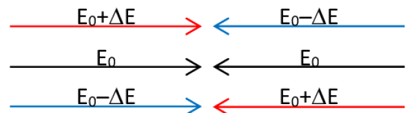
Figure 1: Monochromatization scheme for head-on collisions.

During the following years physicists proposed to upgrade existing colliders or to build new ones based on the same monochromatization principle: VEPP-4Avdienko et al. (1983), Tau-Charm factoryZholents (1992); Faus-Golfe and Le Duff (1992), SPEAR Wille and Chao (1984), B factoryDubrovin and Zholents (1991), LEPBassetti and Jowett (1987). However, the monochromatization principle was never tested.

Recent proposal of monochromatization for FCC-eeValdivia García et al. (2016) was a reason for us to return to the topic of monochromatization in head-on collisions, derive expressions for monochromatization with crossing angle and propose a new monochromatization scheme for crossing angle collisions based on particle’s longitudinal position correlation with energy deviation.

The starting point for our calculations is definition of luminosity $\mathcal{L}$ as a ratio of number of events per second $\dot{N}$ and a total cross section $\sigma$ Møller (1947); Suzuki (1976)

$$\mathcal{L}=\frac{\dot{N}}{\sigma}=f_{0}(1+\cos(2\theta))\int n_{1}n_{2}dVdct\,,$$ (1)

where $f_{0}$ is bunch collision rate, $n_{1}$ and $n_{2}$ are the densities of colliding bunches, $2\theta$ is the full crossing angle (FIG. 2), $V$ is a volume occupied by bunches, $c$ is speed of light and $t$ is time.

II Invariant mass

Collider energy resolution is defined as a square root of second central moment of luminosity distribution with respect to invariant mass $M$. For two colliding particles with four-momenta $P_{1}^{\mu}=\{E_{1},\vec{p}_{1}\}$ and $P_{2}^{\mu}=\{E_{2},\vec{p}_{2}\}$ invariant mass is

$$M^{2}=(P_{1}^{\mu}+P_{2}^{\mu})^{2}=2m_{e}^{2}+2E_{1}E_{2}-2\vec{p}_{1}\vec{p}_{2}\,,$$ (2)

where $\theta$ is a half of the crossing angle (FIG. 2), $E_{1}$, $E_{2}$ and $\vec{p_{1}}$, $\vec{p_{2}}$ are the energies and momenta of two colliding particles, $m_{e}$ is electron mass.

Figure 2: Collision geometry

We will neglect electron mass in further calculations and assume the speed of light $c=1$, therefore energy and momentum are equal $E=\left|\vec{p}\right|$. To calculate the scalar product of momenta we choose accompanying first particle coordinate system with axis $z$ directed along the azimuth of beam orbit

$$\vec{p}_{1} =\{p_{1,x},p_{1,y},p_{1,z}\}\,,$$ (3)

$$\vec{p}_{2} =\{-p_{2,x}^{\prime}\cos(2\theta)+p_{2,z}^{\prime}\sin(2\theta)\,,$$

$$\qquad\;p_{2,y}^{\prime}\,,$$ (4)

$$\qquad\!-p_{2,x}^{\prime}\sin(2\theta)-p_{2,z}^{\prime}\cos(2\theta)\}\,,$$

where the prime variables describe coordinates of the second particle in self accompanying system. Introducing normalized variables $\delta_{1,2}=(E_{(1,2)}-E_{0})/E_{0}$, $x_{1,2}^{\prime}=p_{(1,2),x}/p_{0}$ and $y_{1,2}^{\prime}=p_{(1,2),y}/p_{0}$ we obtain for longitudinal momentum

$$\begin{split}p_{(1,2),z}&=\sqrt{p_{0}^{2}(1+\delta_{(1,2)})^{2}-p_{(1,2),x}^{2}-p_{(1,2),y}^{2}}\\ &=p_{0}\left(1+\delta_{(1,2)}-\frac{x_{(1,2)}^{\prime 2}}{2}-\frac{y_{(1,2)}^{\prime 2}}{2}\right)+O(3)\,,\end{split}$$ (5)

where $E_{0}$ and $p_{0}=E_{0}$ are the average energy and momentum for both bunches. Substituting obtained expression in (2) we obtain

$$\begin{split}M^{2}&=2E_{0}^{2}\biggl{[}(1+\delta_{1}+\delta_{2}+\delta_{1}\delta_{2})(1+\cos(2\theta))\\ &+(x_{2}^{\prime}-x_{1}^{\prime}+x_{2}^{\prime}\delta_{1}-x_{1}^{\prime}\delta_{2})\sin(2\theta)-y1^{\prime}y2^{\prime}\\ &-\left(\frac{x_{1}^{\prime 2}+x_{2}^{\prime 2}+y_{1}^{\prime 2}+y_{2}^{\prime 2}}{2}-x_{1}^{\prime}x_{2}^{\prime}\right)\cos(2\theta)\biggr{]}+O(3)\,.\end{split}$$ (6)

Now, we assume that colliding bunches’ population obey normal distribution with average energy and momentum $E_{0}=\left<E_{1}\right>=\left<E_{2}\right>$ and $E_{0}=p_{0}$, and standard deviation $\sigma_{E}$ with relative value $\sigma_{\delta}=\sigma_{E}/E_{0}$, with angular spreads in vertical and horizontal planes $\sigma_{x^{\prime}}=p_{x^{\prime}}/p_{0}$ and $\sigma_{y^{\prime}}=p_{y^{\prime}}/p_{0}$. We also take a square root of (6) which gives us

$$\begin{split}M&=2E_{0}\biggl{[}\biggl{(}1-\frac{y_{1}^{\prime 2}+y_{2}^{\prime 2}}{4}-\frac{(x_{1}^{\prime}-x_{2}^{\prime})^{2}}{8}\\ &-\frac{(\delta_{1}-\delta_{2})^{2}-4(\delta_{1}+\delta_{2})}{8}\biggr{)}\cos(\theta)+\frac{(y_{1}^{\prime}-y_{2}^{\prime})^{2}}{8\cos(\theta)}\\ &+\frac{2(x_{2}^{\prime}-x_{1}^{\prime})+(\delta_{1}-\delta_{2})(x_{2}^{\prime}+x_{1}^{\prime})}{4}\sin(\theta)\biggr{]}+O(3)\,.\end{split}$$ (7)

Averaging (6) and (7) over angular spreads we derive expressions ready for further use with luminosity distribution:

$$\begin{split}\left<M^{2}\right>_{x^{\prime},y^{\prime}}&=2E_{0}^{2}(1+\delta_{1}+\delta_{2}+\delta_{1}\delta_{2})(1+\cos(2\theta))\\ &-2E_{0}^{2}(\sigma_{x^{\prime}}^{2}+\sigma_{y^{\prime}}^{2})\cos(2\theta)+O(3)\,,\end{split}$$ (8)

$$\begin{split}\left<M\right>_{x^{\prime},y^{\prime}}&=2E_{0}\left[1-\frac{(\delta_{1}-\delta_{2})^{2}}{8}+\frac{\delta_{1}+\delta_{2}}{2}\right]\cos(\theta)\\ &-\frac{E_{0}}{2}\sigma_{x^{\prime}}^{2}\cos(\theta)-\frac{E_{0}}{2}\sigma_{y^{\prime}}^{2}\frac{\cos(2\theta)}{\cos(\theta)}+O(3)\,.\end{split}$$ (9)

III Monochromatization with transverse correlation

A. Renieri Renieri proposed to introduce at IP horizontal dispersion $\pm\psi_{x}$ of opposite signs for colliding beams in head-on collisions. In this case the nature of monochromatization is obvious — collision rate for particles with opposite energy deviation is higher than contrariwise (FIG. 1). Increasing collision angle (zero is head-on) will decrease efficiency of monochromatization but it is still possible (FIG. 3) because particles with energy deviation will meet higher density of the particles with opposite energy deviation.

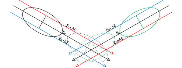
Figure 3: Crossing angle collision with opposite dispersion.

For two colliding bunches (FIG. 4.)

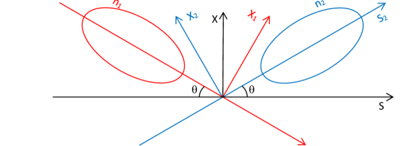
Figure 4: Crossing angle collision with opposite dispersion.

we write the bunch density $n_{i}$ in own frame system

$$\begin{split}n_{i}(x_{i},y_{i},s_{i},t,\delta_{i})&=\frac{N_{i}}{(2\pi)^{4/2}\sigma_{x}\sigma_{y}\sigma_{z}\sigma_{\delta}}\exp\!\left[-\frac{(x_{i}\pm\psi_{x}\delta_{i})^{2}}{2\sigma_{x}^{2}}\right.\\ &\quad\left.-\frac{(y_{i}\pm\psi_{y}\delta_{i})^{2}}{2\sigma_{y}^{2}}-\frac{(s_{i}\mp ct)^{2}}{2\sigma_{z}^{2}}-\frac{\delta_{i}^{2}}{2\sigma_{\delta}^{2}}\right]\,,\end{split}$$ (10)

where we also introduced vertical dispersion $\pm\psi_{y}$ of opposite signs for colliding bunches, $N_{i}$ is bunch population, $\{x_{i},y_{i},s_{i}\}$ is usual accelerator basis of transverse and longitudinal coordinates, $\delta_{i}=(E_{i}-E_{0})/E_{0}$ is energy deviation, and $\sigma_{x,y}=\sqrt{\varepsilon_{x,y}\beta_{x,y}}$, $\varepsilon_{x,y}$, $\beta_{x,y}$ are betatron beam size, emittance and beta function in corresponding plane at the IP, $\sigma_{z}$ and $\sigma_{\delta}$ are standard deviations of bunch longitudinal and energy deviation distributions. Then we need to transform coordinates into laboratory frame with the following expressions

$$\left\{\begin{aligned} x_{i}&=x\cos(\pm\theta)+s\sin(\pm\theta)\,,\\ y_{i}&=y\,,\\ s_{i}&=x\sin(\pm\theta)+s\cos(\pm\theta)\,.\end{aligned}\right.$$ (11)

Using (1) we calculate luminosity according to

$$\begin{split}\mathcal{L}&=f_{0}(1+\cos(2\theta))\times\\ &\times\int n_{1}(x,y,s,t,\delta_{1})n_{2}(x,y,s,t,\delta_{2})dxdydsdctd\delta_{1}d\delta_{2}\,.\end{split}$$ (12)

Neglecting hour glass effect the result is

$$\mathcal{L} =\frac{N_{1}N_{2}}{4\pi\sigma_{x}\sigma_{y}\sqrt{1+\varphi^{2}}}\frac{1}{\Lambda}=\frac{\mathcal{L}_{0}}{\Lambda}\,,$$ (13)

$$\frac{\partial^{2}\mathcal{L}}{\partial\delta_{1}\partial\delta_{2}} =\frac{\mathcal{L}_{0}}{2\pi\sigma_{\delta}^{2}}\exp\left[-\frac{(\delta_{1}-\delta_{2})}{4\sigma_{\delta}^{2}}-\Lambda^{2}\frac{(\delta_{1}+\delta_{2})}{4\sigma_{\delta}^{2}}\right]\,,$$ (14)

$$\Lambda^{2} =1+\frac{\psi_{y}^{2}\sigma_{\delta}^{2}}{\sigma_{y}^{2}}+\frac{\psi_{x}^{2}\sigma_{\delta}^{2}}{\sigma_{x}^{2}(1+\varphi^{2})}\,,$$ (15)

where $\varphi=\sigma_{z}\tan{\theta}/\sigma_{x}$ is Piwinski angle, $\mathcal{L}_{0}$ is luminosity in absence of dispersion Smith (1972). Substitution of zero crossing angle $\theta$ and zero vertical dispersion will give expressions obtained by A. Renieri.

Cross section of the narrow resonance with mass $M_{0}$ could be written as

$$\sigma(\delta_{1},\delta_{2})=B+A\cdot\delta(\left<M\right>_{x^{\prime},y^{\prime}}-M_{0})\,,$$ (16)

where $B$ is describing background and independent of energy, $\left<M\right>_{x^{\prime},y^{\prime}}$ is given in (9). With the help of (1) and (14) the production rate $\dot{N}$ in resonance vicinity is

$$\dot{N} =\int\sigma(\delta_{1},\delta_{2})\frac{\partial^{2}\mathcal{L}}{\partial\delta_{1}\partial\delta_{2}}d\delta_{1}d\delta_{2}$$ (17)

$$=B\frac{\mathcal{L}_{0}}{\Lambda}+A\frac{\mathcal{L}_{0}\exp\left[-\frac{m^{2}\Lambda^{2}}{4E_{0}^{2}\sigma_{\delta}^{2}}\right]}{\sqrt{2\pi}\cos(\theta)\sigma_{\delta}\sqrt{2E_{0}^{2}+E_{0}m\Lambda^{2}}}\,,$$

$$m =\frac{E_{0}}{2}\sigma_{x^{\prime}}^{2}+\frac{E_{0}}{2}\sigma_{y^{\prime}}^{2}\frac{\cos(2\theta)}{\cos(\theta)^{2}}+\frac{M_{0}}{\cos(\theta)}-2E_{0}\,.$$

Calculating expected values of (8) and (9) with (14) we obtain estimation of invariant mass resolution

$$\begin{split}\sigma_{M}^{2}&=\left<M^{2}\right>_{x^{\prime},y^{\prime},\delta_{1},\delta_{2}}-\left<M\right>_{x^{\prime},y^{\prime},\delta_{1},\delta_{2}}^{2}\\ &=2E_{0}^{2}\left[\left(\frac{\sigma_{\delta}\cos(\theta)}{\Lambda}\right)^{2}+\left(\sigma_{x^{\prime}}\sin(\theta)\right)^{2}\right]\,.\end{split}$$ (18)

Note that for large crossing angles the term with angular spread might be dominant.

III.1 Notes on obtaining

For a head-on collisions expression we may further simplify expression for $\Lambda$ (15). First, for $\Lambda\gg 1$ we expand expression (15)

$$\Lambda\approx\frac{\psi\sigma_{\delta}}{\sigma_{x}}\,.$$ (19)

Second, we replace horizontal dispersion in the planar ring at the IP by expression Courant and Snyder (1958)

$$\begin{split}\psi&=\frac{\sqrt{\beta_{x}}}{2\sin(\pi\nu_{x})}\oint\frac{\sqrt{\beta_{x}(\tau)}}{\rho(\tau)}\cos(\varphi(\tau)-\pi\nu_{x})d\tau\\ &=\sqrt{\beta_{x}}F_{D}\,,\\ F_{D}&=\frac{1}{2\sin(\pi\nu_{x})}\oint\frac{\sqrt{\beta_{x}(\tau)}}{\rho(\tau)}\cos(\varphi(\tau)-\pi\nu_{x})d\tau\,,\end{split}$$ (20)

where $\beta_{x}$ is horizontal beta function at the IP, $\rho$ is bending radius of the dipoles, $\varphi(\tau)$ is phase factor, $F_{D}$ is a factor defined by the whole lattice. Third, we substitute expressions for $\sigma_{\delta}$ and $\sigma_{x}=\sqrt{\varepsilon_{x}\beta_{x}}$ with the help of synchrotron radiation integrals Helm et al. (1973)

$$\sigma_{\delta} =\sqrt{C_{q}\gamma^{2}\frac{I_{3}}{J_{s}I_{2}}}\,,$$ (21)

$$\sigma_{x} =\sqrt{C_{q}\gamma^{2}\frac{I_{5}}{J_{x}I_{2}}\beta_{x}}\,,$$ (22)

$$I_{2} =\oint\frac{d\tau}{\rho^{2}(\tau)}\,,$$ (23)

$$I_{3} =\oint\frac{d\tau}{\left|\rho(\tau)\right|^{3}}\,,$$ (24)

$$I_{5} =\oint\frac{\mathcal{H}(\tau)d\tau}{\left|\rho(\tau)\right|^{3}}\,,$$ (25)

where $J_{x}$ and $J_{s}$ are horizontal and longitudinal damping partition numbers, and $\mathcal{H}(s)=\beta_{x}(s)\psi^{\prime 2}(s)+2\alpha_{x}(s)\psi(s)\psi^{\prime}(s)+\gamma_{x}(s)\psi^{2}(s)$. Now then, we obtain expression for $\Lambda$

$$\Lambda\approx F_{D}\sqrt{\frac{J_{x}}{J_{s}}\frac{I_{3}}{I_{5}}}\approx F_{D}\sqrt{\frac{J_{x}}{J_{s}}\frac{1}{\left<\mathcal{H}\right>}}\,,$$ (26)

where $\left<\right>$ denote average value over the ring.

So, in order to obtain large monochromatization factor $\Lambda$ it is necessary to have lattice with small horizontal emittance i.e. small $\left<\mathcal{H}\right>$, horizontal damping partition number greater than longitudinal $J_{x}>J_{s}$, and large lattice factor $F_{D}$(20).

III.2 Example of FCC-ee

Future circular collider (FCC) is a project in CERN of the next accelerator after LHC Benedikt (2016); ref ; Oide et al. (2016). The ultimate goal is 100 km proton-proton machine with 100 TeV central mass energy. The first possible step is $e^{+}e^{-}$ factory — FCC-ee with central mass energy range from 80 GeV to 350 GeV and two IPs. We apply derived expressions of transverse monochromatization scheme to see what luminosity and energy resolution could be achieved at Higgs boson threshold ($\sigma(ee\rightarrow H)=1.6$ fb, $\Gamma=4.2$ MeV, beam energy is $E_{0}=62.5$ GeV).

Influence of synchrotron radiation of the particles in a strong electromagnetic field of the opposite bunch (beamstrahlung) modifies beam emittance, energy spread and length Bogomyagkov et al. (2014). Presence of dispersion at the IP will change beam emittance even more; therefore calculations were performed in steps, on each step new parameters were calculated for a test bunch and then interchanged with parameters of the oncoming bunch until equilibrium is reachedBogomyagkov et al. (2014). Table 1 presents parameters at 62.5 GeV beam energy for baseline (no monochromatization), monochromatization with $\psi=1$ m and $\psi=0.5$ m.

Table 1: Parameters of FCC-ee with and without monochromatization for two IPs.

	Test 0	Test 1	Test 2
Energy, GeV	62.5	62.5	62.5
$\psi_{x}^{*}$, m	0	1	0.5
$\beta_{x}^{*}/\beta_{y}^{*}$, mm	500/1	500/1	500/1.4
$\varepsilon_{x}/\varepsilon_{y}$, nm/pm	0.26/2	2.8/21	3.8/2.9
$\theta$, mrad	15
$\sigma_{x}$, mm	0.01	0.04	0.04
$\sigma_{y}$, $\mu$m	0.04	0.15	0.2
$\sigma_{z}$, mm	8.3	3.8	2.8
$\sigma_{\delta}\,,10^{-4}$	16	7	8
Piwinski angle $\varphi$	11	1.5	0.95
$V_{RF}$, GeV	0.75	0.75	1.5
$N_{p}$	$3\times 10^{11}$
$N_{bunches}$	2615
Luminosity,
$10^{34}$ cm-2s-1	9	2.8	5
$\Lambda$	1	10	6
$\sigma_{M}$, MeV	141	6	11

Notice with $\Lambda=10$ energy resolution improves more than by a factor of ten that is because of energy spread reduction. This happens owing to beamstrahlung: dispersion at the IP increases horizontal emittance (22) and (25), larger emittance means smaller beam density and weaker fields of the opposite bunch; therefore, smaller energy spread. In the last column (Test 2) we increased RF voltage and vertical beta function in order to match the length of interaction area with vertical beta function.

IV Monochromatization with longitudinal correlation

Another approach to enchance collider energy resolution is to use correlation between particle’s longitudinal position and energy (FIG. 5).

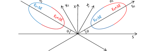
Figure 5: Monochromatization for crossing angle collision with correlation between particle’s energy and longitudinal position.

Such longitudinal correlation may take place in case of strong focusing in longitudinal plain Litvinenko (1997); Gallo et al. (2003a, b). Figure 6 illustrates idea in the phase diagram, where particles belonging to two different ellipses collide when they reach the same $z$ but posses opposite sign of energy deviation.

Figure 6: Colliding beam ellipses in longitudinal plain, showing correlation between collision energy deviation $\delta$ and longitudinal position $z$.

Having $\beta_{z},\alpha_{z},\gamma_{z},\varepsilon_{z}$ Twiss parameters and emittance in longitudinal plain with $\{z=s-ct,\delta\}$ conjugate variables, beam distribution in $\{z,\delta\}$ plain is Kapchinsky and Vladimirsky (1959)

$$f(z,\delta)=\frac{1}{2\pi\varepsilon_{z}}\exp\left[-\frac{\gamma_{z}z^{2}+2\alpha_{z}z\delta+\beta_{z}\delta^{2}}{2\varepsilon_{z}}\right]\,.$$ (27)

In order for monochromatization to happen, the bunches should posses opposite sign of $\alpha_{z}$ (FIG. 6), but because time $s$ flows in opposite direction for the bunches, in further calculations $\alpha_{z}$ has the same sign for both bunches. The bunch density is

$$\begin{split}n_{i}(x_{i},y_{i},z_{i},\delta_{i})&=\frac{N_{i}}{(2\pi)^{4/2}\sigma_{x}\sigma_{y}\varepsilon_{z}}\exp\!\left[-\frac{x_{i}^{2}}{2\sigma_{x}^{2}}\right.\\ &\quad\left.-\frac{y_{i}^{2}}{2\sigma_{y}^{2}}-\frac{\gamma_{z}z^{2}+2\alpha_{z}z\delta+\beta_{z}\delta^{2}}{2\varepsilon_{z}}\right]\,,\end{split}$$ (28)

where $z_{i}=s_{i}\mp ct$. Calculations of luminosity by (12) with coordinate transformation (11) gives similar to (13), (14), (15) results but with different definition of $\Lambda$ and total luminosity is not decreased by $\Lambda$

$$\mathcal{L} =\frac{N_{1}N_{2}}{4\pi\sigma_{x}\sigma_{y}\sqrt{1+\varphi^{2}}}=\mathcal{L}_{0}\,,$$ (29)

$$\frac{\partial^{2}\mathcal{L}}{\partial\delta_{1}\partial\delta_{2}} =\frac{\mathcal{L}_{0}\Lambda}{2\pi\sigma_{\delta}^{2}}\exp\left[-\frac{(\delta_{1}-\delta_{2})}{4\sigma_{\delta}^{2}}-\Lambda^{2}\frac{(\delta_{1}+\delta_{2})}{4\sigma_{\delta}^{2}}\right]\,,$$ (30)

$$\Lambda^{2} =\frac{1+\varphi^{2}}{1+\frac{1}{1+\alpha_{z}^{2}}\varphi^{2}}\approx 1+\alpha_{z}^{2}\,,\quad\varphi\gg 1\,,$$ (31)

where $\sqrt{\varepsilon_{z}\beta_{z}}=\sigma_{z}$, $\sqrt{\varepsilon_{z}\gamma_{z}}=\sigma_{\delta}$, $\varphi=\sqrt{\varepsilon_{z}\beta_{z}}\tan(\theta)/\sigma_{x}$ is Piwinski angle. Note that in case of low $\alpha_{z}$, monochromatization vanishes $\Lambda=1$, which corresponds to the absence of the phase ellipses tilt (FIG. 6) and is a usual state of operation for modern colliders (bunch energy spread and length are independent of $s$).

Production rate at the resonance vicinity with cross section (16) is

$$\dot{N} =\int\sigma(\delta_{1},\delta_{2})\frac{\partial^{2}\mathcal{L}}{\partial\delta_{1}\partial\delta_{2}}d\delta_{1}d\delta_{2}$$ (32)

$$=B\mathcal{L}_{0}+A\frac{\Lambda\mathcal{L}_{0}\exp\left[-\frac{m^{2}\Lambda^{2}}{4E_{0}^{2}\sigma_{\delta}^{2}}\right]}{\sqrt{2\pi}\cos(\theta)\sigma_{\delta}\sqrt{2E_{0}^{2}+E_{0}m\Lambda^{2}}}\,,$$

$$m =\frac{E_{0}}{2}\sigma_{x^{\prime}}^{2}+\frac{E_{0}}{2}\sigma_{y^{\prime}}^{2}\frac{\cos(2\theta)}{\cos(\theta)^{2}}+\frac{M_{0}}{\cos(\theta)}-2E_{0}\,.$$

Comparing production rates for monochromatization with transverse correlation (17) and longitudinal (32) we notice that longitudinal monochromatization is contrary to transverse — background rate is not reduced by $\Lambda$, and production rate of the resonance is increased by $\Lambda$.

Invariant mass resolution is now $s$ dependent and independent of $\alpha_{z}$

$$\begin{split}\sigma_{M}^{2}&=\left<M^{2}\right>_{x^{\prime},y^{\prime},\delta_{1},\delta_{2}}-\left<M\right>_{x^{\prime},y^{\prime},\delta_{1},\delta_{2}}^{2}\\ &=2E_{0}^{2}\left[\left(\frac{\sigma_{\delta}\cos(\theta)}{\Lambda}\right)^{2}+\left(\sigma_{x^{\prime}}\sin(\theta)\right)^{2}\right]\\ &\approx 2E_{0}^{2}\left[\left(\sqrt{\frac{\varepsilon_{z}}{\beta_{z}(s)}}\cos(\theta)\right)^{2}+\left(\sigma_{x^{\prime}}\sin(\theta)\right)^{2}\right]\,.\end{split}$$ (33)

In order to enhance invariant mass resolution one needs to decrease longitudinal emittance and increase beta function at the observation point.

IV.1 Examples of RF focusing

Introduction of Twiss functions in longitudinal plane allowed authors of Gallo et al. (2003a); Chao (1979) to estimate longitudinal emittance

$$\varepsilon_{z}=\sigma_{0\delta}^{2}\frac{\oint\frac{\beta(\tau)}{\left|\rho(\tau)\right|^{3}}d\tau}{\oint\frac{1}{\left|\rho(\tau)\right|^{3}}d\tau}\,,$$ (34)

where $\sigma_{0\delta}^{2}=C_{q}\gamma^{2}I_{3}/(2I_{2})$ is a usual expression for energy spread, $\rho(\tau)$ is bending radius. Obtained expression is similar and could obtained in the same manner as lower fundamental limit on vertical emittance. For a planar isomagnetic ring with the help of (33) we estimate invariant mass resolution

$$\sigma_{M}(s)\approx\sqrt{2}E_{0}\sqrt{\sigma_{0\delta}^{2}\frac{\left<\beta_{z}\right>}{\beta_{z}(s)}\cos^{2}(\theta)+\sigma_{x^{\prime}}^{2}\sin^{2}(\theta)}$$ (35)

where $\left<\beta_{z}\right>$ is average value of longitudinal beta function in the ring. In order to enhance energy resolution we need to minimize $\left<\beta_{z}\right>$ and increase $\beta_{z}$, and minimize $\sigma_{x^{\prime}}\sin(\theta)$.

Authors of Gallo et al. (2003a) studied the case of one cavity and reported a need for high voltage and short wave length RF. We decided to compare one cavity lattice with several cavities lattice. The latter is similar to using more complex cells than FODO in order to achieve lower emittance in transverse plain. For that reason we developed a toy lattice for $2\theta=90$ degree collision angle and with four RF cavities (FIG. 7, TABLE 2), where we chose $\sigma_{x^{\prime}}=0$ to distinguish effect of RF focusing. Introduction of $\sigma_{x^{\prime}}\neq 0$ will worsen invariant mass resolution.

Figure 7: Scetch of RF cavities of the toy ring.

The focusing strength of the cavity is Litvinenko (1997)

$$\frac{1}{F}=\frac{V_{RF}}{E_{0}}\frac{2\pi}{\lambda_{RF}}\,,$$ (36)

where $V_{RF}$ is RF voltage amplitude in the cavity, $\lambda_{RF}$ is wave length of RF field. Since RF amplitude is limited; therefore lower beam energy and shorter wave length are necessary to increase focusing strength of the cavity.

Table 2: Parameters of the toy ring with longitudinal monochromatization.

	Test 0	Test 1	Test 2
Energy, MeV	150
$\Pi$, m	21
$2\theta$, rad	$\pi/2$
$\alpha$	0.5
$U0$, keV	2
$f0$, MHz	14.3
$q1/q2/q3$,	130/13/130
$\sigma_{x}$, $\mu$m	100
$\sigma_{x^{\prime}}\,,10^{-3}$	0
$\sigma_{0\delta}\,,10^{-4}$	4
$V_{RF,1}/V_{RF,2}/V_{RF,3}$, MV	0/0.01/0	0/9/0	-2.9/0.01/2.9
$\varepsilon_{z}$, $10^{-6}$m	33	1	3.3
$\sigma_{\delta,0}/\sigma_{\delta,1}/\sigma_{\delta,2}\,,10^{-4}$	4/4/4	4.9/4.9/4.9	5.3/5.3/5.3
$\sigma_{z,0}/\sigma_{z,1}/\sigma_{z,2}$, mm	81/81/81	2.1/2.4/3.3	7/14/0.6
$\sigma_{M,0}/\sigma_{M,1}/\sigma_{M,2}$, keV	60/60/60	71/63/46	70/35/800

We chose cavity $pF2$ with harmonic factor $q2$ as the one to compensate synchrotron radiation energy loss. The energy spread $\sigma_{\delta}$, bunch length $\sigma_{z}$ and invariant mass resolution $\sigma_{M}$ now depend on the azimuth, the index $\{0,1,2\}$ denotes positions at the beginning of the lattice, at the first and second cavities. Optimizing voltage and harmonic factors of other three cavities we achieved energy resolution almost twice better (Test 2) than in initial state (Test 0) and better than with one cavity (Test 1). The voltage of the additional cavities are 3 MV with frequency of 3 GHz lower than in one cavity case (Test 1). Higher beam energy will require higher voltage and shorter wave length, which now looks unrealistic. However, using more cavities and creating multi cell lattice with longitudinal final focus (like in transverse plain) might produce better monochromatization given that contribution from the term with $\sigma_{x^{\prime}}$ is smaller.

V Conclusion

We derived expressions for energy resolution and luminosity for crossing angle collisions with monochromatization based on transverse and longitudinal correlations between particle position and energy deviation. Monochromatization based on transverse correlation is feasible at the present level of accelerator technology; the longitudinal correlation requires high voltage and high frequency RF system, special longitudinal lattice — hard to build at the present state of RF technology. Introduction of multi cavity lattice reduces requirements for RF system.

- (1) A. Renieri, Possibility of achieving very high energy resolution in electron-positron storage rings, Preprint LNF-75/6(R) (Laboratori Nazionali di Frascati).
- Benedikt (2016) M. Benedikt (2nd FCC week, Rome, 2016).
- (3) FCC-ee design study, Tech. Rep.
- Amman (1976) F. Amman, General formulae of luminosity for various types of colliding beam machines, Preprint KEK-76-3 (National laboratory for high energy physics, 1976).
- Bassetti et al. (1974) M. Bassetti et al., in Proceedings, 9th International Conference on High-Energy Accelerators, Stanford, California, 2-7 May 1974 (1974) pp. 104–107.
- Avdienko et al. (1983) A. A. Avdienko, G. A. Kornyukhin, I. Y. Protopopov, A. N. Skrinsky, A. B. Temnykh, G. M. Tumaikin, and A. A. Zholents, Proceedings, 12th International Conference on High-Energy Accelerators, HEACC 1983: Fermilab, Batavia, August 11-16, 1983, Conf. Proc. C830811, 186 (1983).
- Zholents (1992) A. A. Zholents, Polarized J / psi mesons at a tau charm factory with a monochromator scheme, Tech. Rep. CERN-SL-92-27-AP (1992).
- Faus-Golfe and Le Duff (1992) A. Faus-Golfe and J. Le Duff, A Versatile lattice for a tau - charm factory that includes a monochromatization scheme, Tech. Rep. LAL-RT-92-01 (1992).
- Wille and Chao (1984) K. Wille and A. W. Chao, INVESTIGATION OF A MONOCHROMATOR SCHEME FOR SPEAR, Tech. Rep. SLAC/AP-032, SLAC/AP-32 (1984).
- Dubrovin and Zholents (1991) A. N. Dubrovin and A. A. Zholents, Conference Record of the 1991 IEEE Particle Accelerator Conference (PAC 1991): Accelerator Science and Technology May 6-9, 1991 San Francisco, California, Conf. Proc. C910506, 2835 (1991), [,2835(1991)].
- Bassetti and Jowett (1987) M. Bassetti and J. M. Jowett, Proceedings of the 1987 IEEE Particle Accelerator Conference (PAC1987): Accelerator Engineering and Technology, March 16-19, 1987 Washington, D.C., Conf. Proc. C870316, 115 (1987).
- Valdivia García et al. (2016) M. A. Valdivia García, A. Faus-Golfe, and F. Zimmermann, in Proceedings, 7th International Particle Accelerator Conference (IPAC 2016): Busan, Korea, May 8-13, 2016 (2016) p. WEPMW009.
- Møller (1947) C. Møller, in Proceedings, International Conference on Fundamental Particles and Low Temperatures, vol.1, Cambridge, UK, 22-27 Jul 1946 (1947) pp. 194–199.
- Suzuki (1976) T. Suzuki, General formulae of luminosity for various types of colliding beam machines, Preprint KEK-76-3 (National laboratory for high energy physics, 1976).
- Smith (1972) L. Smith, On the calculation of luminosity for electron - proton colliding beam, Tech. Rep. PEP-0020, LBL-ERAN-191 (1972).
- Courant and Snyder (1958) E. D. Courant and H. S. Snyder, Annals Phys. 3, 1 (1958), [Annals Phys.281,360(2000)].
- Helm et al. (1973) R. H. Helm, M. J. Lee, P. L. Morton, and M. Sands, 1973 particle accelerator conference. accelerator engineering and technology. San Francisco, March 1973, IEEE Trans. Nucl. Sci. 20, 900 (1973).
- Oide et al. (2016) K. Oide et al., Phys. Rev. Accel. Beams 19, 111005 (2016), arXiv:1610.07170 [physics.acc-ph] .
- Bogomyagkov et al. (2014) A. Bogomyagkov, E. Levichev, and D. Shatilov, Phys. Rev. ST Accel. Beams 17, 041004 (2014), arXiv:1311.1580 [physics.acc-ph] .
- Litvinenko (1997) V. N. Litvinenko, in Nonlinear and collective phenomena in beam physics. Proceedings, Workshop of the International Committee on Future Accelerators, Arcidosso, Italy, September 2-6, 1996, Vol. 395 (1997) pp. 275–283, [,275(1996)].
- Gallo et al. (2003a) A. Gallo, P. Raimondi, and M. Zobov, in 30th Advanced ICFA Beam Dynamics Workshop on High Luminosity e+ e- Collisions (e+ e- Factories 2003) Stanford, California, October 13-16, 2003, Vol. C0309101 (2003) p. THWA003, arXiv:physics/0404020 [physics] .
- Gallo et al. (2003b) A. Gallo, P. Raimondi, and M. Zobov, Strong RF focusing for luminosity increase, Tech. Rep. DAFNE-TECHNICAL-NOTE:-G-60 (2003) arXiv:physics/0309066 [physics] .
- Kapchinsky and Vladimirsky (1959) I. Kapchinsky and V. Vladimirsky, in Proceedings II International Conference on High Energy Accelerators, Geneva, Cern, 1959 (1959) pp. 274–288.
- Chao (1979) A. W. Chao, J. Appl. Phys. 50, 595 (1979).