October 31, 2016
Mean Field Voter Model of Election to the House of Representatives in Japan
Abstract
In this study, we propose a mechanical model of a plurality election based on a mean field voter model. We assume that there are three candidates in each electoral district, i.e., one from the ruling party, one from the main opposition party, and one from other political parties. The voters are classified as fixed supporters and herding (floating) voters with ratios of and , respectively. Fixed supporters make decisions based on their information and herding voters make the same choice as another randomly selected voter. The equilibrium vote-share probability density of herding voters follows a Dirichlet distribution. We estimate the composition of fixed supporters in each electoral district and using data from elections to the House of Representatives in Japan (43rd to 47th). The spatial inhomogeneity of fixed supporters explains the long-range spatial and temporal correlations. The estimated values of are close to the estimates obtained from a survey.
1 Introduction
Social phenomena are an active research field in econophysics and socio-physics, and many studies have aimed to deepen our understanding of them[1, 2, 3, 4]. Opinion dynamics is a central research theme and voter models have been studied extensively as a paradigm of opinion dynamics[5, 6, 7, 8]. Recently, the validity of a model was tested for describing the real opinion dynamics in the U.S. presidential election[9], where it was concluded that a noisy diffusive process of opinions can reproduce the statistical features of elections, i.e., the stationary vote-share distributions and long-range spatial correlation, which decay logarithmically with distance. The model is simple and attractive in the domain of physics.
In the model, the decisions made by all the voters are described by an infection mechanism. Two voters are selected randomly and one voter’s choice is made the same as another’s choice, with some noise. The spatial inhomogeneity of the system is considered by using data to define the initial conditions. The noise level has to be fine tuned in order to simulate the statistical properties of elections, particularly maintaining the initial spatial inhomogeneity; otherwise, the spatial pattern disappears or the spatial correlation becomes too strong and the model cannot reproduce the statistical properties of the election data. However, it is necessary to avoid making subtle choices for the parameters when modeling a social system. If people interact with others and make decisions in a social system, the process should be robust and stable. This is the first problem that needs to be addressed.
The second problem is estimating the ratio of floating voters who do not vote for a particular political party. In the voter model described above, the opinions of all the voters can be changed by interactions with other voters. However, this approach is too simple to represent the situation in actual elections. Some people prefer a certain political party and it is reasonable to assume that their opinions will not be changed easily by interacting with others. Nowadays, many people recently have become dissatisfied with the current status of the political system and they have no particular political party to vote for[11]. They are called floating voters and it is considered that they have a decisive role in the results of elections. If we assume that social interactions play a crucial role in their decisions [9, 3, 10], then they should be studied in the framework of a voter model.
In the present study, we propose a mean field voter model to describe the dynamics of a plurality election in Japan. In the model, voters are classified as fixed supporters who have a preference for a specific political party and floating voters whose decision depends on the choices of others. The influence of other voters on floating voters is described by the voter model mechanism. The vote share distribution of floating voters follows a Dirichlet distribution and the system is stable. We show how to decompose the vote share into votes by fixed supporters and those by floating voters, and we estimate the spatial inhomogeneity of the electoral system. We study the fluctuations in the vote share of floating voters and the ratio of floating voters is estimated. We explain the spatial correlation and temporal correlation in terms of the spatial inhomogeneity in the fixed supporters.
2 Mean Field Voter Model
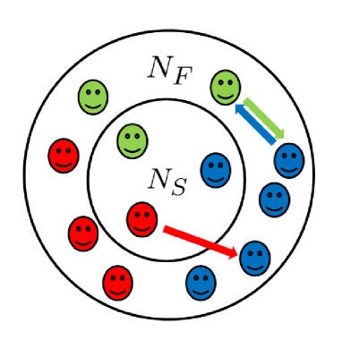
There are political parties, electoral districts, and elections. In each election, candidates fight for a single congress seat in each electoral district. We denote the political parties as , electoral districts as , and elections as . There are votes in district for election , and voters vote for political party . holds. are classified as floating (herding) voters and fixed supporters who vote for political party (Figure 1). and we denote the total floating voters and supporters as and , respectively. We write the ratio of floating voter as , . We denote the vote share for political party as . is then decomposed as
We introduce , which represents the vote share of political party among fixed supporters. The ratio is denoted as , which represents the vote share of political party among floating voters.
| (1) |
We assume that the choices of fixed supporters do not change and that the choices of floating voters are described by a voter model. In each turn, a randomly selected floating voter changes his choice to that of another randomly selected voter. The fixed supporters only affect the choices made by floating voters. We also assume that among fixed supporters, only supporters can affect the choices of floating voters. As shown in the following, controls the fluctuations in from .
At equilibrium, variables with values in the standard unit interval add up to 1, , which constrains the sample space of dependent variables to a dimensional simplex. Thus, one variable can always be omitted due to . We use the abbreviated form of and . The probability density of is described by a Dirichlet distribution, which is given by Eq. (2). We employ the alternative parametrization of the Dirichlet distribution introduced by Ferrari and Cribari-Neto[12]. The derivation is given in Appendix B.
| (2) |
The denominator in eq.(2) is the multinomial beta function, which serves as a normalization constant, and it is defined as
is the gamma function defined as .
We write the random variable obeys the Dirichlet distribution in the alternative parametrization as
Each component of is marginally beta-distributed with and . The expected values are defined as , the variances are , and the covariances are . is a “precision” parameter to model the dispersion of the variables. In the context of the mean field voter model, a small indicates that the influence is weak and the fluctuations in are large. If is large, the influence is strong and the fluctuations in from are suppressed, and almost coincides with .
3 Data Analysis
| date | Districts | Regions | Voters | Votes | Ruling Political Party | |
|---|---|---|---|---|---|---|
| 1 | 2003/11/9 | 300 | 3345 | LDP | ||
| 2 | 2005/9/11 | 300 | 2534 | LDP | ||
| 3 | 2009/8/30 | 300 | 2037 | LDP | ||
| 4 | 2012/12/16 | 300 | 1994 | DPJ | ||
| 5 | 2014/12/14 | 295 | 1983 | LDP |
We employ data from elections to the House of Representatives (general election) in Japan. This is a plurality election and there are about 300 electoral districts, where several candidates compete for a single congress seat. We use data of elections from the 43rd (2003) to 47th (2014) elections, which we label as and in Table 1. During this period, the Liberal Democratic party of Japan (LDP) and the Democratic party of Japan (DPJ) were elected as the ruling party in and elections and election, respectively. As there is only one congress seat in each electoral district, there is at most one candidate from each of these two political parties. We label the candidates from LDP as and from DPJ as . There might be several candidates from other political parties (OPP), we combine them together and treat them as one candidate. We label them as . By this treatment of several candidates from OPP, there are at most three candidates in each district. Each district is divided into several regions where the results of the elections were recorded. There are 2000 to 3000 regions.
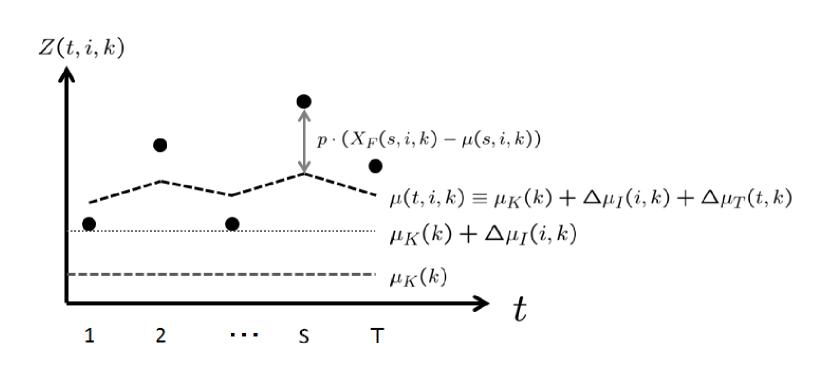
We use data from the regions where the above three candidates fought for a single seat five times in a row due to the necessity to infer in the mean field voter model. There are regions, which we label as . We denote the vote share for candidate in region in election as . holds in region in election . In order to decompose as described in Eq. (1), we write as
shows the different types of fitness values for the politicians from political party . Please refer to Figure 2. shows the overall fitness, and and show the temporal and regional deviation from , respectively. shows the fitness of a candidate from political party in region in election .
| Number of political parties and their index | |
| Number of elections and time variable | |
| Number of regions and their index | |
| Number of votes in region for election | |
| for political party | |
| Votes share for political party in region for election | |
| Number of floating voters and fixed supporters in region , election | |
| Ratio of floating voter | |
| for political party | |
| Vote share of political party among fixed supporters | |
| Overall fitness of political party | |
| Temporal deviation of fitness from , | |
| Regional deviation of fitness from , | |
| for political party | |
| Vote share of political party among floating voters | |
| Number of fixed supporters who can affect the choices of floating voters. |
We summarize the notations in Table 2. The decomposition is similar to ANOVA (analysis of variance ) in statistics. There are three factors, and and we assume there is no interaction effect among them and are estimated as the sum of the three factors, and . In the next section, we use the maximum likelihood principle to estimate the model parameters. Based on the results, we test the validity of the mean field voter model.
4 Results
We assume that the floating voter ratio does not depend on region and write it as . In the mean field voter model, are decomposed as,
| (3) |
There are parameters in the model, which we estimate using the maximum likelihood principle. When we apply the maximum likelihood principle, some becomes negative for small values of . In this case, we assume that . is estimated as . Table 3 shows the results for in the first row. We also show the number of cases where we employed in the second row. For about one-third of cases, at least one of for each becomes negative by the choice in election . Thus, the estimate of is not appropriate or the assumption that is independent of is too crude.
| 1 | 2 | 3 | 4 | 5 | |
|---|---|---|---|---|---|
| 146 | 124 | 132 | 78 | 142 | |
| NHK poll |
We also show the estimates obtained by Japan Broadcasting Corporation (NHK) in the third row, which are based on a public poll of more than 1000 people[14]. According to the poll, 25% to 39% are estimated as floating voters. The estimate obtained by the mean field voter model is in the same order.
4.1 vs and standardized
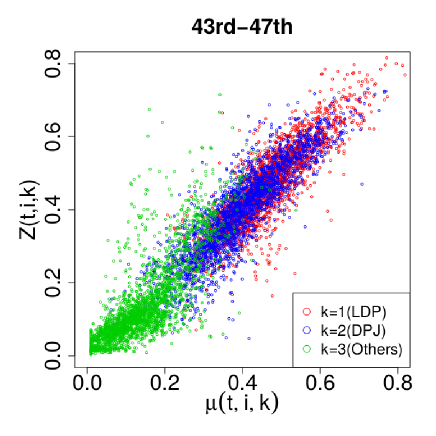
We show the scatter plots for and in Figure3. If the decomposition in Eq. (1) is correct, then is distributed around . As shown in Figure 3, for and are distributed almost symmetrically around the diagonal. However, the distribution of is not symmetric around the diagonal, so the decomposition might not be good for the candidates with .
 |
 |
 |
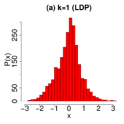
In order to check the validity of the proposed model, we estimate the standardized , which is denoted as . If the model is correct and holds, then V. is defined as
| (4) |
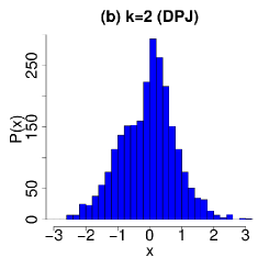
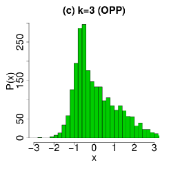
Figure 4 shows the probability densities for with , respectively. The variances in are estimated as , and for , respectively. As shown in Figure 4, the distribution with is wider than those with . does not follow a normal distribution, so the asymmetrical nature of the distribution is not crucial. However, the variance with is about the twice that with , which suggests that the decomposition in Eq. (1) is not good. We discuss improvements to the proposed model in the conclusion.
4.2 Spatial and temporal correlations
 |
 |
 |
We estimate the spatial and temporal correlations. The spatial correlation function is computed as
| (5) |
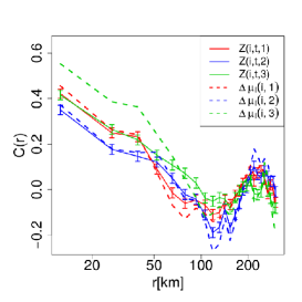
The first term is averaged over pairs of regions separated by a distance . The spatial correlation decays logarithmically with geographical distance [Figure 5(a)], as reported in previous studies. The logarithmic decay of the spatial correlations is considered generic for the fluctuations in electoral dynamics[9]. In the figure, we also plot the correlation functions for , which clearly almost coincide with for . This suggests that the physical description of the spatial correlation is spatial inhomogeneity in . Every region has certain characteristics, such as the type of the region and its historical nature. These characteristic do not change rapidly even if some people move between regions. If all the voters are floating voters[9], the diffusion and noise should be controlled to maintain the inhomogeneity in . In our model, the voters are classified as fixed supporters and floating voters, and there is no movement of people among different regions, so it is not necessary to consider this issue.
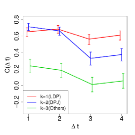
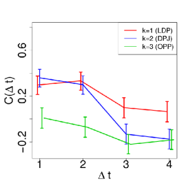
Figure 5(b) shows the results for the temporal correlation, , which is computed as
| (6) |
Here is defined as . does not decay with , which can be explained by the decomposition in Eq. (1). The covariance of and is decomposed into the covariance of and , and the covariance of and .
We assume that and are independent from each other. If we further assume that the correlation between and decays with , as and do not depend on , we have
Then, the temporal correlation for a large value of is approximately expressed as
| (7) |
which suggests that the physical origin of the temporal correlation is also the spatial inhomogeneity of .
We also check the decomposition in Eq. (1) by studying the temporal correlation of . Figure 5(c) shows it, which is defined by replacing with in eq. (6). decays with and it almost vanishes for . However, becomes negative for and . This suggests that a more subtle decomposition of should be performed.
5 Conclusions
In this study, we proposed a mean field voter model for a plurality election. We assumed that voters are classified as fixed supporters and floating voters, where the behavior of the latter can be described by the voter model’s infection mechanism. We decomposed the vote share into that from the fixed supporters and that from the floating voters , . has three factors and . follows a Dirichlet distribution with the parameters . We estimated the model parameter , where we used electoral data from the House of Representatives elections in Japan during 2003–2014. There we assume that does not depend on the region and there is no interaction effect among the three factors in . Using the estimated parameters, we decomposed and checked the validity of the proposed model.
-
•
The variances in the standardized are , and for , respectively (Figure 4).
-
•
The spatial correlation functions for are described by those for (Figure 5(a)).
- •
These results show that the decomposition of is effective for simulating the statistical nature of the electoral data. However, the decomposition should be performed carefully to verify the validity of the mean field voter model. We estimated using some average values of , which should be replaced with the maximum likelihood estimates. In addition, the assumption of the independence of on is also excessively crude and it is necessary to consider their regional dependencies. These issues should be addressed in future studies.
Appendix A Election Data
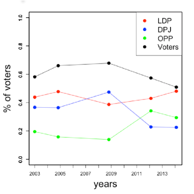
We provide further information regarding the data discussed in the main text. We used the results of House of Representatives elections from 2003 (43rd) to 2014 (47th), which were aggregated into electoral districts[13]. In Figure6(a), we present the global features of the election data, i.e., the turnout as well as votes for the LDP, DPJ, and OPP. In Figure 6(b), we show the changes in the shares associated with the turnout and the votes for different parties in the regions considered in the main text. There are regions. The shares were computed region-by-region, and we then extracted the averages and standard deviations.
 |
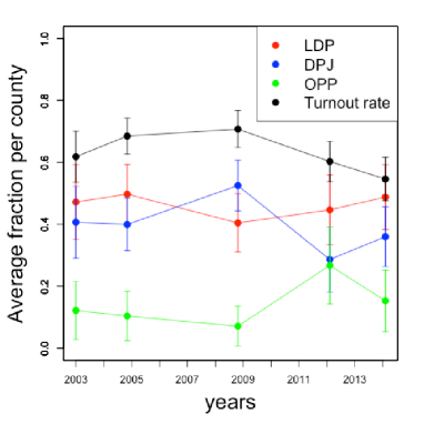 |
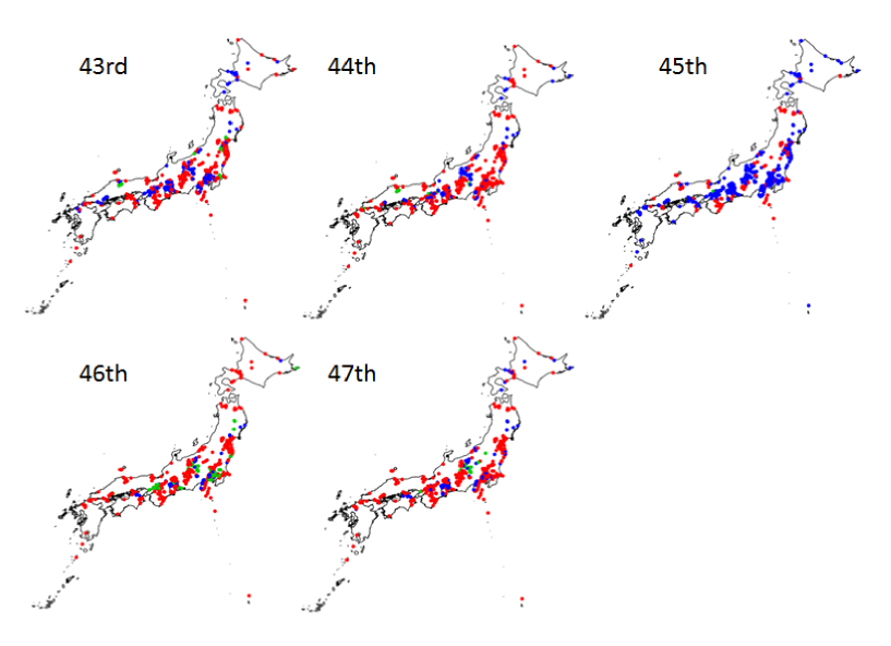
Figure 7 shows the winning political party in electoral regions during five general elections.
Appendix B
We derive the Dirichlet distribution for . There are floating voters and voters for political party . . We write the probability function as . The proportion of fixed supporters affects the choices of the floating voters because there are voters. The probability that a randomly selected voter is a floating voter with choice is . The probability that another randomly chosen voter makes the choice is . The transition probability from state for any pair is given as
Similarly, the transition probability from state is given as
The detailed balance condition for the stationary can be solved easily and we obtain
where . In the limit , the probability function becomes a Dirichlet distribution.
References
- [1] R. N. Mantegna and H. E. Stanley, Introduction to Econophysics: Correlations and Complexity in Finance (Cambridge University Press, Cambridge, 2007).
- [2] A. Pentland, Social Physics: How good ideas spread (Penguin Press, 2014).
- [3] P. Ormerod, Positive Linking, (Faber & Faber, 2012).
- [4] S. Mori, K. Nakayama and M. Hisakado : Phys. Rev. E.94(2016)052301.
- [5] C. Castellano, S. Fortunato, and V. Loreto: Rev. Mod. Phys.81(2009)591.
- [6] S. Mori and M. Hisakado: J. Phys. Soc. Jpn.79(2010)034001.
- [7] M. Hisakado and S. Mori, J. Phys. A43(2010)315207.
- [8] S. Mori, M. Hisakado, and T. Takahashi: Phys. Rev. E.86(2012)026109.
- [9] J. Fernandez-Gracia, K. Suchecki, J. J. Ramasco, M. San Miguel, and V. M. Eguíluz: Phys. Rev. Lett 112(2014)158701.
- [10] N. A. Ara jo, J. S. Andrade, and H. J. Herrmann: PLoS One 5(2010)e12446.
- [11] L. Killan, The Swing Vote: The Untapped Power of Independents (St. Martin’s Press, 2012).
- [12] S. P. L. Ferrari and F. Cribari-Neto: Journal of Statistical Software 34(2004)799.
- [13] S. Mizusaki and Y. Mori, JED-M Ver 3.2 28th-47th general elections regional data (LDP press, 2015)
- [14] Japan Broadcasting Corporation (NHK) conducts public opinion polls by telephone every month to examine political consciousness of the people. The survey target is male and female over the age of 20 nationwide and the investigation method is the telephone method (RDD tracking method). One can get the data from the website, https://www.nhk.or.jp/bunken/research/yoron/political/2016.html. The data contain several political parties’ support rate and the ratio of people who do not have a specific political party to support.