Hidden correlations entailed by q-non additivity render the q-monoatomic gas highly non trivial

A. Plastino1, M. C. Rocca1
, 1 La Plata National University and Argentina’s National Research Council
(IFLP-CCT-CONICET)-C. C. 727, 1900 La Plata - Argentina
Abstract

It ts known that Tsallis’ q-non-additivity entails hidden correlations. It has also been shown that even for a monoatomic gas, both the q-partition function $Z$ and the mean energy $<U>$ diverge and, in particular, exhibit poles for certain values of the Tsallis non additivity parameter $q$. This happens because $Z$ and $<U>$ both depend on a $\Gamma$-function. This $\Gamma$, in turn, depends upon the spatial dimension $\nu$. We encounter three different regimes according to the argument $A$ of the $\Gamma$-function. (1) $A>0$, (2) $A<0$ and $\Gamma>0$ outside the poles. (3) $A$ displays poles and the physics is obtained via dimensional regularization. In cases (2) and (3) one discovers gravitational effects and quartets of particles. Moreover, bound states and gravitational effects emerge as a consequence of the hidden q-correlations.

Keywords: q-Statistics, divergences, partition function, dimensional regularization, specific heat.

1 Introduction

Generalized or q-statistical mechanics Γ  la Tsallis has generated manifold applications in the last quarter of a century [1, 2, 3, 4, 5, 6, 7, 8, 9, 10, 11, 12, 13]. It has been shown (see for instance, [14, 15]) that Tsallis’ q-statistics is of great importance for dealing with some astrophysical issues involving self-gravitating systems [16]. Moreover, this statistics has proved its utility in many different scientific fields, with several thousands of publications and authors [2], so that studying its structural features is an important issue for physics, astronomy, biology, neurology, economics, etc. [1]. The success of the q-statistics reaffirms the well grounded notion asserting that there is much physics whose origin is of purely statistical nature (not mechanical). As a spectacular example, me mention the application of q-ideas to high energy experimental physics, where the q-statistics appears to adequately describe the transverse momentum distributions of different hadrons [17, 18, 19].

In this work we show that as yet unexplored gravitational effects characterize this q-theory on account of divergences that, in some circumstances, emerge, within the q-statistical framework, in both the mean energy $<U>$ and the partition function $Z$ [20].

Divergences constitute an important issue in theoretical physics. Indeed, the study and elimination of divergences of a physical theory is perhaps one of the most important aspects of theoretical work. The quintessential typical example is the thus far failed, attempt to quantify the gravitational field. Some examples of elimination of divergences can be looked at in references [21, 22, 23, 24, 25].

We will use here an extremely simplified version, such as that of [26], of the ideas of [21, 22, 23, 24, 25] in connection with Tsallis q-statistics [1, 2], with emphasis in its applicability to gravitational issues [14, 15], in particular self-gravitating systems [16]. We will see that the removal of the above mentioned divergences produces interesting insights.

It is to be stressed that for $Z<0$ the system can not exist, as no probabilities can be introduced. Then, several options are available. $<U>>0$ is the natural state of affairs. We will uncover that, in a Tsallis’ scenario, $<U><0$ is possible for special q-values which entails boundedness. Also negative specific heats $C$ may emerge, an indication of gravitational effects [16].

These interesting results appear after using mathematics known since at least 40 years ago and for whose development M. Veltman and G. t’Hooft where awarded the Nobel prize of physics in 1999. Acquaintance with such mathematics is not really needed to understand this paper. The reader has merely to accept that their physical significance can not be doubted. In a few words, one needs from the above mathematics analytical extensions and dimensional regularization [21, 22, 23, 24, 25].

In this work we analyze the behavior of $Z$ and $<U>$ in three regions of the argument of the $\Gamma$-function contained in them. The nature of the argument of the $\Gamma$-function governs the behavior of $Z$ and $<U>$. This behavior yields three different regions, for a given spatial dimension $\nu$, Tsallis’ index $q$ and number of particles $N$. The region’s particularities are:
$(1)\;\;\;\frac{1}{1-q}-\frac{n\nu}{2}-1>0$
$(2)\;\;\;\frac{1}{1-q}-\frac{n\nu}{2}<0\;\;\;\Gamma\left(\frac{1}{1-q}-\frac{n\nu}{2}\right)>0$
$(3)\;\;\;\frac{1}{1-q}-\frac{n\nu}{2}=-p\;\;\;p=0,1,2,3,4.....$
Normal monoatomic gas behavior is encountered in region (1). Instead, gravitational effects are discovered in region (2). Finally, in region (3) we have both normal behavior and gravitational effects. In particular the $N$ particles are grouped into quartets that remind one of alpha particles. It should be noted than in case (3) we are making a regularization of the corresponding theory and NOT a renormalization.

2 The monoatomic gas

We stress that here we use normal (linear in the probability) expectation values, and not the weighted ones usually attached to Tsallis’ theory [1]. This is done for simplicity. Other ways of evaluating mean values pose difficulties in this context that will be tackled in the future [28].

Remark that in this case, restricting ourselves to the interval $[0<q\leq 1]$, the so-called Tsallis cut-off [1] does not apply.

The q-partition function of a monoatomic gas is given by:

$$Z=V^{n}\int\limits_{-\infty}^{\infty}\left[1+\frac{\beta(1-q)}{2m}(p_{1}^{2}+p_{2}^{2}+\cdot\cdot\cdot p_{n}^{2})\right]^{\frac{1}{q-1}}d^{\nu}p_{1}d^{\nu}p_{2}\cdot\cdot\cdot d^{\nu}p_{n},$$ (2.1)

The mean energy is defined by:

$$<U>=\frac{V^{n}}{Z}\int\limits_{-\infty}^{\infty}\left[1+\frac{\beta(1-q)}{2m}(p_{1}^{2}+p_{2}^{2}+\cdot\cdot\cdot p_{n}^{2})\right]^{\frac{1}{q-1}}$$
$$\frac{p_{1}^{2}+p_{2}^{2}+\cdot\cdot\cdot p_{n}^{2}}{2m}d^{\nu}p_{1}d^{\nu}p_{2}\cdot\cdot\cdot d^{\nu}p_{n}.$$ (2.2)

Both integrals are in general divergent for many values of $q$. This can be proved by a simple powers count. We appeal to techniques developed in [21, 22, 23, 24, 25] so as to deal with them.

In ref.[26] we have computed both $Z$ and $<U>$ obtaining:

$$Z=V^{n}\left[\frac{2\pi m}{\beta(1-q)}\right]^{\frac{\nu n}{2}}\frac{\Gamma\left(\frac{1}{1-q}-\frac{\nu n}{2}\right)}{\Gamma\left(\frac{1}{1-q}\right)}.$$ (2.3)
$$<U>=\frac{V^{n}}{Z}\frac{\nu n}{2\beta(1-q)}\left[\frac{2\pi m}{\beta(1-q)}\right]^{\frac{\nu n}{2}}\frac{\Gamma\left(\frac{1}{1-q}-\frac{\nu n}{2}-1\right)}{\Gamma\left(\frac{1}{1-q}\right)}.$$ (2.4)
$$<U>=\frac{\nu n}{\beta[2q-\nu n(1-q)]}.$$ (2.5)

The derivative with respect to $T$ yields for the specific heat at constant volume

$$C_{V}=\frac{\nu nk}{2q-\nu n(1-q)}.$$ (2.6)

3 Limitations for the particle-number

We briefly review now results obtained in Ref. [26]. Some related work by Livadiotis, McComas, and Obregon, should be cited [12, 13, 27]. We pass first to analyze the Gamma functions involved in computing $Z$ and $<U>$, for the region $[0<q\leq 1]$. From (2.3) we have, for positive Gamma-argument

$$\frac{1}{1-q}-\frac{\nu n}{2}>0.$$ (3.1)

In the same vein we have from (2.4)

$$\frac{1}{1-q}-\frac{\nu n}{2}-1>0.$$ (3.2)

We reach then two conditions that pose severe limitations on the particle-number $n$, i.e.,

$$1\leq n<\frac{2q}{\nu(1-q)}$$ (3.3)

There is a maximum permissible $n$. For example, if $q=1-10^{-3},\nu=3$, one has

$$1\leq n<666.$$ (3.4)

We can not have more than 665 particles. Keeping the dimensionality equal to three, for $q=1/2$ just one particle is permitted and for $q=1/4$, no particles can be present exist. Roughly, for a number of particles of the order of $10^{n}$, $q$ has to be of the order of $1-10^{-n}$.

4 The dimensional analytical extension of divergent integrals [21, 22, 23, 24, 25]

The exposition of our present results starts here. We pass first to considering negative Gamma arguments in (2.3), which will require analytical extension/dimensional regularization in integrals (2.1) and (2.2). One has

$$\frac{1}{1-q}-\frac{\nu n}{2}<0,$$ (4.1)

together with

$$\Gamma\left(\frac{1}{1-q}-\frac{\nu n}{2}\right)>0,$$ (4.2)

We use now

$$\Gamma(z)\Gamma(1-z)=\frac{\pi}{\sin(\pi z)},$$ (4.3)

to find

$$\Gamma\left(\frac{1}{1-q}-\frac{\nu n}{2}\right)=-\frac{\pi}{\sin\pi\left(\frac{\nu n}{2}-\frac{1}{1-q}\right)\Gamma\left(\frac{\nu n}{2}-\frac{1}{1-q}\right)}>0.$$ (4.4)

This is true if

$$\sin\pi\left(\frac{\nu n}{2}-\frac{1}{1-q}\right)<0,$$ (4.5)

so that

$$2p+1<\frac{\nu n}{2}-\frac{1}{1-q}<2(p+1)$$ (4.6)

where $p=0,1,2,3,4,5.....$, or equivalently

$$\frac{4p+2}{\nu}+\frac{2}{\nu(1-q)}<n<\frac{4(p+1)}{\nu}+\frac{2}{\nu(1-q)}.$$ (4.7)

Now, from (2.3), (2.5), and (2.6) we obtain (a) $Z>0$, (b) $<U><0$, (c) $C<0$, which entails bound states, on account of (b) and self-gravitation according to (c) [16].

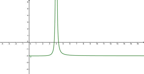
5 The poles of the q-Ideal Gas treatment

If the Gamma’s argument is such that

$$\frac{1}{1-q}-\frac{\nu n}{2}=-p\;\;{\rm for}\;\;p=0,1,2,3,......,$$ (5.1)

$Z$ displays a single pole.

For $\nu=1$ we have

$$\frac{1}{1-q}-\frac{n}{2}=-p\;\;{\rm for}\;\;p=0,1,2,3,.......$$ (5.2)

Since $0\leq q<1$, the concomitant $q$ values are

$$q=\frac{1}{2},\frac{2}{3},\frac{3}{4},\frac{4}{5},......,$$ (5.3)

$n$ even, $n\geq 4$ and

$$q=\frac{1}{3},\frac{3}{5},\frac{5}{7},\frac{7}{9},......,$$ (5.4)

$n$ odd, $n\geq 3$.

For $\nu=2$

$$\frac{1}{1-q}-n=-p\;\;{\rm for}\;\;p=0,1,2,3,......,$$ (5.5)

Again, since $0\leq q<1$,

$$q=\frac{1}{2},\frac{2}{3},\frac{3}{4},\frac{4}{5},......,$$ (5.6)

$n\geq 2$.

For $\nu=3$

$$\frac{1}{1-q}-\frac{3n}{2}=-p\;\;{\rm for}\;\;p=0,1,2,3,......,$$ (5.7)

and because $0\leq q<1$,

$$q=\frac{1}{2},\frac{2}{3},\frac{3}{4},\frac{4}{5},......,$$ (5.8)

$n$ even, $n\geq 1$, and

$$q=\frac{1}{3},\frac{3}{5},\frac{5}{7},\frac{7}{9},......,$$ (5.9)

$n$ odd, $n\geq 1$.

The location of these poles will change if escort mean values where used.
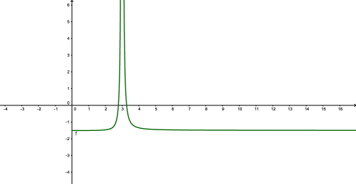
We discuss now poles in $<U>$, given by

$$\frac{1}{1-q}-\frac{\nu n}{2}-1=-p\;\;{\rm for}\;\;p=0,1,2,3,......,$$ (5.10)

For $\nu=1$

$$\frac{1}{1-q}-\frac{n}{2}-1=-p\;\;{\rm for}\;\;p=0,1,2,3,......,$$ (5.11)

On account on the condition (G): $0\leq q<1$ we have

$$q=\frac{1}{2},\frac{2}{3},\frac{3}{4},\frac{4}{5},......,$$ (5.12)

for $n$ even, $n\geq 2$ and

$$q=\frac{1}{3},\frac{3}{5},\frac{5}{7},\frac{7}{9},......,$$ (5.13)

for $n$ odd , $n\geq 1$.

For $\nu=2$

$$\frac{1}{1-q}-n-1=-p\;\;{\rm for}\;\;p=0,1,2,3,......,$$ (5.14)

minding (G) we have

$$q=\frac{1}{2},\frac{2}{3},\frac{3}{4},\frac{4}{5},......,$$ (5.15)

$n\geq 1$.

For $\nu=3$

$$\frac{1}{1-q}-\frac{3n}{2}-1=-p\;\;{\rm for}\;\;p=0,1,2,3,......,$$ (5.16)

and, from (G),

$$q=\frac{1}{2},\frac{2}{3},\frac{3}{4},\frac{4}{5},......,$$ (5.17)

$n$ even, $n\geq 1$ and

$$q=\frac{1}{3},\frac{3}{5},\frac{5}{7},\frac{7}{9},......,$$ (5.18)

$n$ odd, $n\geq 1$.

6 The three-dimensional case

As an example of dimensional regularization [21, 22, 23, 24, 25] we will go into some detail concerning the poles at $q=\frac{1}{2}$ and $q=\frac{1}{3}$.

6.1 The $q=1/2$ pole

In this case $n$is even, $n\geq 2$. We have

$$Z=V^{n}\left(\frac{4m\pi}{\beta}\right)^{\frac{\nu n}{2}}\Gamma\left(2-\frac{\nu n}{2}\right).$$ (6.1)

Using

$$\Gamma\left(2-\frac{\nu n}{2}\right)\Gamma\left(\frac{\nu n}{2}-1\right)=-\frac{\pi}{\sin\left(\frac{\pi\nu n}{2}\right)}$$ (6.2)

or, equivalenly

$$\Gamma\left(2-\frac{\nu n}{2}\right)\Gamma\left(\frac{\nu n}{2}-1\right)=-\frac{(-1)^{\frac{3n}{2}+1}\pi}{\sin\left[\frac{\pi n}{2}(\nu-3)\right]},$$ (6.3)

so that

$$Z=V^{n}\left(\frac{4m\pi}{\beta}\right)^{\frac{\nu n}{2}}\frac{(-1)^{\frac{3n}{2}+1}\pi}{\sin[\frac{\pi n}{2}(\nu-3)]\Gamma\left(\frac{\nu n}{2}-1\right)}.$$ (6.4)

Since

$$\sin[\frac{\pi n}{2}(\nu-3)]=\frac{\pi n}{2}(\nu-3)\left\{1+\sum\limits_{m=1}^{\infty}\frac{(-1)^{m}}{(2m+1)!}\left[\frac{\pi n}{2}(\nu-3)\right]^{2m}\right\}=$$ (6.5)
$$=\frac{\pi n}{2}(\nu-3)X,$$ (6.6)

with

$$X=\left\{1+\sum\limits_{m=1}^{\infty}\frac{(-1)^{m}}{(2m+1)!}\left[\frac{\pi n}{2}(\nu-3)\right]^{2m}\right\},$$ (6.7)

we get

$$Z=V^{n}\left(\frac{4m\pi}{\beta}\right)^{\frac{3n}{2}}\frac{(-1)^{\frac{3n}{2}+1}}{\Gamma\left(\frac{\nu n}{2}-1\right)X\frac{n}{2}(\nu-3)}\left[1+\frac{n}{2}(\nu-3)\ln\left(\frac{4m\pi}{\beta}\right)+\cdot\cdot\cdot\right]$$ (6.8)

The term independent of $\nu-3$ is, following dimensional regularization prescriptions [21, 22, 23, 24, 25]

$$Z=V^{n}\left(\frac{4m\pi}{\beta}\right)^{\frac{3n}{2}}\frac{(-1)^{\frac{3n}{2}+1}}{\Gamma\left(\frac{3n}{2}-1\right)}\ln\left(\frac{4m\pi}{\beta}\right)$$ (6.9)

This is then the physical Z-value at the pole [21, 22, 23, 24, 25]. For the mean energy we have

$$Z<U>=V^{n}\frac{n\nu}{\beta}\left(\frac{4m\pi}{\beta}\right)^{\frac{\nu n}{2}}\Gamma\left(1-\frac{\nu n}{2}\right).$$ (6.10)

Using

$$\Gamma\left(1-\frac{\nu n}{2}\right)\Gamma\left(\frac{\nu n}{2}\right)=\frac{\pi}{\sin\left(\frac{\pi\nu n}{2}\right)}$$ (6.11)

or, equivalently

$$\Gamma\left(1-\frac{\nu n}{2}\right)\Gamma\left(\frac{\nu n}{2}\right)=-\frac{(-1)^{\frac{3n}{2}}\pi}{\sin\left[\frac{\pi n}{2}(\nu-3)\right]}$$ (6.12)

one finds for $<U>$

$$Z<U>=V^{n}\frac{n\nu}{\beta}\left(\frac{4m\pi}{\beta}\right)^{\frac{\nu n}{2}}\frac{(-1)^{\frac{3n}{2}}\pi}{\sin[\frac{\pi n}{2}(\nu-3)]\Gamma\left(\frac{\nu n}{2}\right)}.$$ (6.13)

$<U>$ can be recast as

$$Z<U>=V^{n}\frac{n(\nu-3)}{\beta}\left(\frac{4m\pi}{\beta}\right)^{\frac{\nu n}{2}}\frac{(-1)^{\frac{3n}{2}}\pi}{\sin[\frac{\pi n}{2}(\nu-3)]\Gamma\left(\frac{\nu n}{2}\right)}+$$
$$V^{n}\frac{3n}{\beta}\left(\frac{4m\pi}{\beta}\right)^{\frac{\nu n}{2}}\frac{(-1)^{\frac{3n}{2}}\pi}{\sin[\frac{\pi n}{2}(\nu-3)]\Gamma\left(\frac{\nu n}{2}\right)}.$$ (6.14)

Repeating the Z-treatment yields for $<U>$:

$$Z<U>=V^{n}\frac{2}{\beta}\left(\frac{4m\pi}{\beta}\right)^{\frac{3n}{2}}\frac{(-1)^{\frac{3n}{2}}}{\Gamma\left(\frac{3n}{2}\right)}+$$
$$V^{n}\frac{3n}{\beta}\left(\frac{4m\pi}{\beta}\right)^{\frac{3n}{2}}\frac{(-1)^{\frac{3n}{2}}}{\Gamma\left(\frac{3n}{2}\right)}\ln\left(\frac{4m\pi}{\beta}\right)$$ (6.15)

or, equivalently

$$Z<U>=V^{n}\frac{2}{\beta}\left(\frac{4m\pi}{\beta}\right)^{\frac{3n}{2}}\frac{(-1)^{\frac{3n}{2}}}{\Gamma\left(\frac{3n}{2}\right)}\left[1-\frac{3n}{2}\ln\left(\frac{4m\pi}{\beta}\right)\right].$$ (6.16)

Appealing here to (6.9) for the physical $Z$ we finally obtain

$$<{\cal U}>=\frac{4}{\beta(3n-2)}\left[\frac{1}{\ln\beta-\ln 4m\pi}-\frac{3n}{2}\right].$$ (6.17)

We discuss first $(-1)^{\frac{3n}{2}+1}=-1$ and then $n=4,8,12,16......$, so that

$$Z=\frac{V^{n}}{\Gamma\left(\frac{3n}{2}-1\right)}\left(\frac{4m\pi}{\beta}\right)^{\frac{3n}{2}}\ln\left(\frac{\beta}{4m\pi}\right)$$ (6.18)

If $(-1)^{\frac{3n}{2}+1}=1$, then $n=2,6,10,14......$ and

$$Z=\frac{V^{n}}{\Gamma\left(\frac{3n}{2}-1\right)}\left(\frac{4m\pi}{\beta}\right)^{\frac{3n}{2}}\ln\left(\frac{4m\pi}{\beta}\right).$$ (6.19)

From (6.17) - (6.18) and requiring $Z>0$ and $<U>>0$ one deduces

$$\frac{1}{4m\pi ke^{\frac{2}{3n}}}<T<\frac{1}{4m\pi k}.$$ (6.20)

From (6.17) - (6.19) and demanding $Z>0$ y $<U><0$ one finds

$$0\leq T<\frac{1}{4m\pi ke^{\frac{2}{3n}}}$$ (6.21)

The specific heat derives from (6.17) for $<U>$. One has

$$C=\frac{4k}{3n-2}\left[\frac{1}{\ln\beta-\ln 4m\pi}+\frac{1}{(\ln\beta-\ln 4m\pi)^{2}}-\frac{3n}{2}\right].$$ (6.22)

6.2 The $q=1/3$ pole

Here $Z$ is

$$Z=V^{n}\left(\frac{3m\pi}{\beta}\right)^{\frac{\nu n}{2}}\frac{\Gamma\left(\frac{3}{2}-\frac{\nu n}{2}\right)}{\Gamma\left(\frac{3}{2}\right)}.$$ (6.23)

Using again

$$\Gamma\left(\frac{3}{2}-\frac{\nu n}{2}\right)\Gamma\left(\frac{\nu n}{2}-\frac{1}{2}\right)=-\frac{\pi}{\cos\left(\frac{\pi\nu n}{2}\right)},$$ (6.24)

or, equivalently

$$\Gamma\left(\frac{3}{2}-\frac{\nu n}{2}\right)\Gamma\left(\frac{\nu n}{2}-\frac{1}{2}\right)=-\frac{(-1)^{\frac{3n-1}{2}}\pi}{\sin\left[\frac{\pi n}{2}(\nu-3)\right]},$$ (6.25)

so that

$$Z=\frac{V^{n}}{\Gamma\left(\frac{3}{2}\right)}\left(\frac{3m\pi}{\beta}\right)^{\frac{\nu n}{2}}\frac{(-1)^{\frac{3n-1}{2}}\pi}{\sin[\frac{\pi}{2}(\nu-3)]\Gamma\left(\frac{\nu n}{2}-\frac{1}{2}\right)}.$$ (6.26)

We can dimensionally regularize $Z$ - $<U>$ as above, to find

$$Z=\frac{V^{n}}{\Gamma\left(\frac{3n}{2}\right)}\left(\frac{3m\pi}{\beta}\right)^{\frac{3n}{2}}\frac{(-1)^{\frac{3n-1}{2}}}{\Gamma\left(\frac{3n-1}{2}\right)}\ln\left(\frac{3m\pi}{\beta}\right),$$ (6.27)
$$<{\cal U}>=\frac{3}{\beta(3n-1)}\left[\frac{1}{\ln\beta-\ln 3m\pi}-\frac{3n}{2}\right].$$ (6.28)

We tackle first $(-1)^{\frac{3n-1}{2}}=-1$ and then $n=1,5,9,13......$

$$Z=\frac{V^{n}}{\Gamma\left(\frac{3}{2}\right)\Gamma\left(\frac{3n-1}{2}\right)}\left(\frac{3m\pi}{\beta}\right)^{\frac{3n}{2}}\ln\left(\frac{\beta}{3m\pi}\right).$$ (6.29)

For $(-1)^{\frac{3n-1}{2}}=1$, then $n=3,7,11,15......$

$$Z=\frac{V^{n}}{\Gamma\left(\frac{3}{2}\right)\Gamma\left(\frac{3n-1}{2}\right)}\left(\frac{3m\pi}{\beta}\right)^{\frac{3n}{2}}\ln\left(\frac{3m\pi}{\beta}\right).$$ (6.30)

From (6.28) - (6.29) and demanding e $Z>0$ - $<U>>0$ we find

$$\frac{1}{3m\pi ke^{\frac{2}{3n}}}<T<\frac{1}{3m\pi k}.$$ (6.31)

From (6.28)-y (6.30) and requiring $Z>0$ - $<U><0$ we get

$$0\leq T<\frac{1}{3m\pi ke^{\frac{2}{3n}}}.$$ (6.32)

Finally, for $C$ one has

$$C=\frac{3k}{3n-1}\left[\frac{1}{\ln\beta-\ln 3m\pi}+\frac{1}{(\ln\beta-\ln 3m\pi)^{2}}-\frac{3n}{2}\right].$$ (6.33)

7 Conclusions

We have used an elementary regularization procedure to investigate the poles in both $Z$ and $<U>$ for specific, discrete q-values, in Tsallis’ q-scenario. We analyzed the thermal behavior at the poles and encountered suggestive features. The study was undertaken in one, two, three, and $N$ dimensions. Amongst the ensuing pole-features, rather unexpected, but nonetheless true, we focus on:

  • β€’

    There is an upper bound to the temperature at the poles, re-confirming the discoveries of Ref. [29].

  • β€’

    In some instances, Tsallis’ entropies are positive just for a restricted temperature-range.

  • β€’

    Negative specific heats, characteristic feature of self-gravitating systems [16], are found. See the illuminating by Silva-Alcaniz [30]. We will, in a future work, try to connect our methodology with that of this reference.

Our physical results are deduced only from statistics and not from mechanical properties. This fact brings to mind of a similar feature that emerges in the case of the entropic force conjectured by Verlinde [31].

References

  • [1] M. Gell-Mann and C. Tsallis, Eds. Nonextensive Entropy: Interdisciplinary applications, Oxford University Press, Oxford, 2004; C. Tsallis, Introduction to Nonextensive Statistical Mechanics: Approaching a Complex World, Springer, New York, 2009.
  • [2] See http://tsallis.cat.cbpf.br/biblio.htm for a regularly updated bibliography on the subject.
  • [3] I. S. Oliveira: Eur. Phys. J. B 14, 43 (2000)
  • [4] E. K. Lenzi , R. S. Mendes: Eur. Phys. J. B 21, 401 (2001)
  • [5] C. Tsallis: Eur. Phys. J. A 40, 257 (2009)
  • [6] P. H. Chavanis: Eur. Phys. J. B 53, 487 (2003)
  • [7] G. Ruiz ,C. Tsallis: Eur. Phys. J. B 67, 577 (2009)
  • [8] P. H. Chavanis , A. Campa: Eur. Phys. J. B 76, 581 (2010)
  • [9] N. Kalogeropoulos: Eur. Phys. J. B 87, 56 (2014)
  • [10] N. Kalogeropoulos: Eur. Phys. J. B 87, 138 (2014)
  • [11] A. Kononovicius, J. Ruseckas: Eur. Phys. J. B 87, 169 (2014)
  • [12] G. Livadiotis, D. J. McComas: APJ 748, 88 (2011).
  • [13] G. Livadiotis: Entropy 17, 2062 (2015).
  • [14] A. R. Plastino, A. Plastino, Phys. Lett. A 174 (1993) 384.
  • [15] P. H. Chavanis, C. Sire, Physica A 356 (2005) 419; P.-H. Chavanis, J. Sommeria, Mon. Not. R. Astron. Soc. 296 (1998) 569.
  • [16] D. Lynden-Bell, R. M. Lynden-Bell, Mon. Not. R. Astron. Soc. 181 (1977) 405.
  • [17] C. Tsallis, Introduction to Nonextensive Statistical Mechanics (Springer, Berlin, 2009).
  • [18] F. Barile et al. (ALICE Collaboration), EPJ Web Conferences 60, (2013) 13012; B. Abelev et al. (ALICE Collaboration), Phys. Rev. Lett. 111, (2013) 222301; Yu. V.Kharlov (ALICE Collaboration), Physics of Atomic Nuclei 76, (2013) 1497. ALICE Collaboration, Phys. Rev. C 91, (2015) 024609; ATLAS Collaboration, New J. Physics 13, (2011) 053033; CMS Collaboration, J. High Energy Phys. 05, (2011) 064; CMS Collaboration, Eur. Phys. J. C 74, (2014) 2847.
  • [19] A. Adare et al (PHENIX Collaboration), Phys. Rev. D 83, (2011) 052004; PHENIX Collaboration, Phys. Rev. C 83, (2011) 024909; PHENIX Collaboration, Phys. Rev. C 83, (2011) 064903; PHENIX Collaboration, Phys. Rev. C 84, (2011) 044902.
  • [20] A. Plastino; M. C. Rocca; G. L. Ferri: EPJB 89, 150 (2016).
  • [21] C. G. Bollini and J. J. Giambiagi: Phys. Lett. B 40, (1972), 566.Il Nuovo Cim. B 12, (1972), 20.
  • [22] C. G. Bollini and J.J Giambiagi : Phys. Rev. D 53, (1996), 5761.
  • [23] G.’t Hooft and M. Veltman: Nucl. Phys. B 44, (1972), 189.
  • [24] C. G. Bollini, T. Escobar and M. C. Rocca : Int. J. of Theor. Phys. 38, (1999), 2315.
  • [25] C. G Bollini and M.C. Rocca : Int. J. of Theor. Phys. 43, (2004), 59. Int. J. of Theor. Phys. 43, (2004), 1019. Int. J. of Theor. Phys. 46, (2007), 3030.
  • [26] A. Plastino, M. C. Rocca: arXiv:1701.03525
  • [27] O. Obregon, International Journal of Modern Physics A 30 (2015) 1530039.
  • [28] E. P. Bento et al. Phys. Rev. E 91, (2015) 022105. G. Baris Bagcy and Thomas Oikonomou. Phys. Rev. E 92 (2015) 016103.
  • [29] A. R. Plastino, A. Plastino, Phys. Lett. A 193 (1994) 140.
  • [30] R. Silva and J. R. Alcaniz. Phys. Lett. A 313 (2003) 393.
  • [31] E. Verlinde, arXiv:1001.0785 [hep-th]; JHEP 04, 29 (2011).
Refer to caption
Figure 1: $c/k$ at the pole $q=1/2$ versus $\beta$ for $m=1/\pi$ and $n=100$. The right branch corresponds to $Z>0$, i.e., the physical branch.
Refer to caption
Figure 2: $c/k$ at the pole $q=1/3$ versus $\beta$, for $m=1/\pi$ and $n=99$. The right branch corresponds to $Z>0$, i.e., the physical branch.