Spin memory effect for compact binaries in the post-Newtonian approximation

Abstract

The spin memory effect is a recently predicted relativistic phenomenon in asymptotically flat spacetimes that become nonradiative infinitely far in the past and future. Between these early and late times, the magnetic-parity part of the time integral of the gravitational-wave strain can undergo a nonzero change; this difference is the spin memory effect. Families of freely falling observers around an isolated source can measure this effect, in principle, and fluxes of angular momentum per unit solid angle (or changes in superspin charges) generate the effect. The spin memory effect had not been computed explicitly for astrophysical sources of gravitational waves, such as compact binaries. In this paper, we compute the spin memory in terms of a set of radiative multipole moments of the gravitational-wave strain. The result of this calculation allows us to establish the following results about the spin memory: (i) We find that the accumulation of the spin memory behaves in a qualitatively different way from that of the displacement memory effect for nonspinning, quasicircular compact binaries in the post-Newtonian approximation: the spin memory undergoes a large secular growth over the duration of the inspiral, whereas for the displacement effect this increase is small. (ii) The rate at which the spin memory grows is equivalent to a nonlinear, but nonoscillatory and nonhereditary effect in the gravitational waveform that had been previously calculated for nonspinning, quasicircular compact binaries. (iii) This rate of build-up of the spin memory could potentially be detected by future gravitational-wave detectors by carefully combining the measured waveforms from hundreds of gravitational-wave detections of compact binaries.

I Introduction

I.1 Overview of the displacement memory effect

The displacement memory effect is a well studied property of asymptotically flat spacetimes that limit to nonradiative solutions infinitely far in the past and future. The effect is characterized by the gravitational-wave strain undergoing a change between these early and late times. Nearby freely falling observers can measure this effect through their geodesic deviation. In principle, any isolated source that radiates (effective) energy density in massless (or gravitational) fields asymmetrically, or that has a change in its supermomentum charges, can produce the effect. It is of great interest to know whether astrophysical sources that exist in our observable universe can generate the effect with a sufficient amplitude so that it might be detected by current or upcoming gravitational-wave experiments.

Zel’dovich and Polnarev Zel’dovich and Polnarev (1974) made an important first step in this direction when they computed, in linearized gravity, the displacement memory arising from the scattering of stars. Related calculations of the displacement memory from gravitational bremsstrahlung were performed soon after Turner (1977); Turner and Will (1978); Kovacs and Thorne (1978). Turner also noted that neutrino emission from supernovae would be a source of the displacement memory effect Turner (1978). These early calculations of the effect were all in the context of linear gravity. Christodoulou Christodoulou (1991) found that the effective energy per solid angle radiated in gravitational waves could also be a source of the displacement memory, in principle. Wiseman and Will Wiseman and Will (1991) calculated this nonlinear displacement memory for compact binaries, and Blanchet and Damour Blanchet and Damour (1992) computed the effect in the post-Newtonian-expanded, multipolar post-Minkowski approximation (henceforth, the PN approximation, for short). They were able to confirm that compact binaries do have a nontrivial memory effect. The displacement memory effect has subsequently been computed to a high order in the PN approximation Favata (2009a) and in numerical relativity simulations Pollney and Reisswig (2011) (comparisons between numerical and analytical calculations of the displacement memory are given in Cao and Han (2016)).

With a range of astrophysical sources that generate the displacement memory and with the improvement in the sensitivity of current gravitational-wave detectors, observing the displacement memory is now an active goal of gravitational-wave research. Initial strategies to detect the displacement memory signal were proposed as long as roughly thirty years ago Braginsky and Grishchuk (1985); Braginskii and Thorne (1987). Pulsar timing experiments have performed searches for the displacement memory, though they have not yet found evidence for the phenomenon Wang et al. (2015); Arzoumanian et al. (2015). In addition, it will be possible to use LIGO Abbott et al. (2009) (alone or in concert with Virgo Acernese et al. (2015) and KAGRA Aso et al. (2013)) to detect the accumulation of the displacement memory by coherently combining on the order of one-hundred memory signals from gravitational-wave detections of binary black holes Lasky et al. (2016). Future ground-based gravitational-wave detectors will be able to observe the displacement memory in even greater detail, and space-based interferometers, such as the LISA mission Audley et al. (2017), would be capable of detecting the memory signal from individual supermassive-binary-black-hole mergers Favata (2009b).

The displacement memory also has an interesting connection to the symmetry group of asymptotically flat spacetimes, the Bondi-Metzner-Sachs group Bondi et al. (1962); Sachs (1962, 1962). This group has a similar structure to the Poincaré group, in the sense that it is the semidirect product of an abelian group with a group isomorphic to the proper, orthochronous Lorentz group; however, rather than having a four-dimensional group of translations, it has an infinite-dimensional group of supertranslations (which include the four-dimensional group of ordinary translations). The additional supertranslations, roughly, can be thought of as “angle-dependent” translations. The displacement memory is related to the supertranslation needed to reach a particular frame at late times from a related frame at early times (see, e.g., Strominger and Zhiboedov (2016a); Flanagan and Nichols (2017) for recent descriptions of this property). Alternatively, it can be thought of as the transformation needed to transform a “preferred” Poincaré group at early times to a different preferred Poincaré group at late times (e.g., Ashtekar (2014)). Finally, there is one additional interesting relationship between the memory and asymptotic symmetries: the changes in charges conjugate to the supertranslations, the supermomentum charges, are also a source of the displacement memory.

I.2 Summary of the spin memory

The history of the spin memory has unfolded following a somewhat different path. Its discovery was inspired (at least in part) by the work of Barnich and Troessaert Barnich and Troessaert (2010a, b) (see also Banks (2003)). In these papers, they proposed that the symmetry algebra of asymptotically flat spacetimes be enlarged to incorporate all symmetry vector fields, including those that have analytic singularities. This extends the Lorentz part of the algebra to the Virasoro algebra with vanishing central charge. The additional generators were dubbed “super-rotations,” because they can be thought of as generalizations of the Lorentz vector fields (very roughly, they are a certain type of angle-dependent rotations and boosts).

Several years later, Pasterski et al. Pasterski et al. (2015) observed that there is a new memory effect that is related to the super-rotation symmetry, though in a somewhat different way from how the displacement memory and the supertranslation symmetry are related (see also Flanagan and Nichols (2017)). This new memory was dubbed the “spin memory,” because it is sourced by asymmetric changes in the (effective) angular momentum per unit solid angle radiated to null infinity in massless (and gravitational) fields, as well as changes in the superspin charges (the magnetic-parity part of the charges conjugate to the super-rotation vector fields). However, it has no relation to a spacetime super-rotated from a specific early-time frame, because such spacetimes are not asymptotically flat in the traditional sense (see, e.g., Strominger and Zhiboedov (2016b))

There are (at least) two idealized observational methods by which the spin memory can be measured: (i) Construct a set of Bondi coordinates around an isolated source and require that an observer follow an accelerating worldline of constant spatial Bondi coordinates. Have this observer carry a Sagnac detector and have her measure the time-integrated change in the Sagnac effect between early and late times. The resulting change is the spin memory Pasterski et al. (2015). (ii) Consider a family of freely falling observers around an isolated source. Have them measure their geodesic deviation from their neighboring observers and allow them to compare their results with these other observers around the source. From these measurements they can extract the magnetic-parity portion of the sky pattern of the time-integrated strain that defines the spin memory Flanagan et al. (2017). Both (i) and (ii) are in fact nonlocal measurements, because some nonlocal information is hidden in the procedure to define Bondi coordinates.

There is, therefore, compelling theoretical evidence that, in principle, the spin memory exists and is measurable. However, there are neither any calculations of the magnitude of the effect from astrophysical sources, nor are there explicit strategies to detect the spin memory using current or future gravitational-wave detectors. This paper is a first step towards addressing these gaps in our understanding of the spin memory. Our focus will be on compact binary systems in quasicircular orbits which, given the recent detections of black-hole binaries by the LIGO-Virgo Collaboration Abbott et al. (2016a), are a particularly relevant and promising source.

Computing the spin memory in full generality from such sources would be challenging and would likely require the computational infrastructure of Cauchy numerical relativity simulations combined with Cauchy-characteristic extraction (e.g., Bishop et al. (1996); Reisswig et al. (2009); Handmer et al. (2016)). We will not attempt such a large undertaking in this paper. Instead, we will derive an expression for the spin memory in terms of a set of radiative multipole moments of the gravitational-wave strain. Within the PN approximation, we can then relate the radiative moments to a set of source moments and thereby obtain quantitative values for the magnitude of the growth of the spin memory from specific types of astrophysical sources (in particular, compact binaries in quasicircular orbits).

I.3 Methodology for computing memory effects

In the Bondi framework, the displacement memory can be computed from one component of Einstein’s equations (which turns out to contain equivalent information to the flux law for the supermomentum charges). The contributions to the displacement memory can be categorized into three types: changes in the supermomentum charges (the ordinary displacement memory in the nomenclature of Bieri and Garfinkle (2014)), fluxes of the stress-energy tensor of matter fields (the matter part of the null displacement memory), and fluxes of the effective stress-energy of gravitational fields (the nonlinear null displacement memory). These contributions are defined in terms of quantities far from an isolated source without reference to quantities in the interior of the spacetime. The displacement memory effect is then the limiting change of the gravitational-wave strain produced by these three contributions, between the asymptotically nonradiative regions of the spacetime infinitely far in the past and future.

The PN approximation takes a different approach to defining the displacement memory effect. Because the PN approach perturbatively relates the dynamics of a source to its emitted gravitational waves via an asymptotic matching calculation, it cannot describe the complete evolution of a compact binary; the errors in the perturbative expansion grow large when the binary’s separation is small. It is not possible to use the PN approximation until the binary settles into the asymptotically nonradiative state in the future that is needed to define the displacement memory effect. Instead a proxy for the displacement memory is defined in PN theory by a specific piece of the PN-expanded wave-zone metric perturbation at a fixed time, which is not instantaneous (nonhereditary) and nonlinear and resembles the retarded integral of the effective energy density of the gravitational field (see, e.g., Blanchet (2014)). Specifically, this contribution is the nonlinear part of the null displacement memory, in the terminology of Bieri and Garfinkle (2014). It is also this piece of the metric that serves as the displacement memory signal that can be detected by gravitational-wave detectors (such as LIGO Lasky et al. (2016)) rather than the formal asymptotic change in the gravitational-wave strain.

In the Bondi framework, the spin memory has contributions from three types of sources that are analogous to those of the displacement memory: there is an ordinary part from changes of the superspin charges, a matter part of the null spin memory from the flux of angular momentum per solid angle in matter fields, and a nonlinear null spin memory from the flux of effective angular momentum per solid angle in gravitational waves. In the PN framework, the spin memory has not been computed, and there is not yet an established definition of what the spin memory observable is in this approximation. We will define the spin memory in this context by its nonlinear null part evaluated at a finite retarded time, rather than infinitely far in the future (analogously to how the displacement memory is defined in PN theory). The features of this definition of the spin memory are described next.

I.4 Summary of results

Our results are based on an expression for the spherical-harmonic modes of the spin memory observable that we compute in this paper in terms of the radiative multipole moments of the gravitational-wave strain. From this expression, we can determine the spin memory for nonspinning quasicircular compact binaries in the PN approximation. For these systems, we will denote the total mass of the binary by $M$ and its orbital frequency by $\omega$. We will form the dimensionless PN quantity $x=(M\omega)^{2/3}$ (in geometric units in which $G=c=1$). Our calculations show that the spin memory is contained predominantly in the $l=3$, $m=0$ mode (for a coordinate frame in which the binary has its orbital angular momentum oriented along the $z$ direction). This mode scales as $x^{-1/2}$; namely, it gradually accumulates over the long inspiral to have a quite significant effect. One should contrast this with the displacement memory, which scales as $x$ (it grows most rapidly when the binary is most relativistic and has small contributions from the early stages of the inspiral).

While this difference in scaling at low orbital frequencies is indeed a curiosity, it is difficult to envision how to observe this feature directly. The gradual accumulation of the spin memory takes place over such a long timescale that for any individual event, it is difficult to envision a way to measure this effect. LIGO, for example, is sensitive to just the late stages of the inspiral (and the merger and ringdown) of stellar-mass compact binaries, and it measures the strain, not its time integral. This would seem to pose a challenge for detecting the spin memory. However, we are able to show that the rate at which the spin memory accumulates is equivalent to a nonlinear, nonhereditary, and nonoscillatory component of the gravitational waveform that had previously been discovered at 2.5 PN order for nonspinning compact binaries Arun et al. (2004). For this reason, we will subsequently call this term the “spin memory mode.” This quantity is conceivably detectable, although its high PN order would make it challenging to do so.

To estimate the spin memory mode’s detectability, we use improvised (though nonrigorous) waveforms created by inserting numerical-relativity gravitational-waveform modes from the SXS waveform catalog SXS into the leading PN-order multipolar expression we derive for the spin memory. For individual binary mergers, we find that the signal-to-noise ratio (SNR) in the spin memory component of the waveform is below the detection threshold. However, by coherently combining the spin memory signals using a procedure similar to that described in Lasky et al. (2016), we suspect that the effect could be measurable by future ground-based detectors like the Einstein Telescope (see, e.g., Punturo et al. (2010)).

I.5 Outline of this paper

We structure the remainder of our paper in the following way: In Sec. II, we describe the basic elements of the PN approximation and the Bondi framework. It is here that we describe a way to incorporate a set of PN radiative moments into a Bondi frame. As a warm up, we show in Sec. III that we can use this PN-expanded Bondi frame to correctly predict the multipolar expression for the PN computation of the displacement memory, including the correct leading-order expression for the PN displacement memory of compact binary systems. With this result completed, we then turn to the calculation of the nonlinear part of the null spin memory in Sec. IV. We give both a general expression in terms of the radiative moments of the gravitational-wave strain and a leading-order result for compact binaries in this section. We also show how the rate of accumulation of the spin memory corresponds to the 2.5PN nonlinear, nonoscillatory, and nonhereditary part of the gravitational waveform (the spin memory mode). In Sec. V, we estimate the SNR of the spin memory mode in current and future ground-based detectors. We sketch a procedure for coherently adding spin memory signals to allow for the detection of this phenomenon. In Sec. VI, we conclude. Appendix A contains certain properties of the vector and tensor spherical harmonics that appear in our calculations. As a check of our calculation of the spin memory, we show in Appendix B that we recover the same expression for the flux of angular momentum flux expanded in multipole moments of the gravitational-wave strain that was derived in Thorne (1980) using very different methods. Finally, in Appendix C, we compare the spin memory mode in a numerical simulation with our improvised, approximate waveform model.

Throughout this paper, we use units in which $G=c=1$, although we will on occasion denote relative PN errors with expressions of the form $O(c^{-n})$ where $c$ is the speed of light and $O(G^{m})$ for Newton’s constant $G$. Our conventions for the metric and curvature tensors follow those given in Wald Wald (1984).

II Elements of the Bondi and PN frameworks

In the two parts of this section, we introduce the minimal elements of the PN approximation and the Bondi framework that we will need for this paper. More detailed reviews of PN theory can be found, for example, in Blanchet (2014). The textbook by Stewart Stewart (1994), for example, has significantly more information about asymptotically flat spacetimes, as does the recent review article Mädler and Winicour (2016a).

II.1 PN approximation

Our focus will be primarily on the asymptotic gravitational waveform within the PN approximation, and our emphasis in this section, therefore, will largely fall on this aspect of PN theory.

II.1.1 General aspects of PN theory

The gravitational waveform in the PN approximation is encoded within a symmetric, trace-free and transverse tensor $h_{ij}^{\mathrm{TT}}$. We are using the notation that the Latin indices $i$ and $j$ refer to spatial indices in inertial Minkowski coordinates. The transverse-traceless metric perturbation is a function of two sets of radiative multipole moments, which are often called the mass and current moments. We will expand $h_{ij}^{\mathrm{TT}}$ in sets of second-rank, “pure-spin” tensor harmonics of electric and magnetic parity. The definitions of these harmonics and their relationship to the spin-weighted spherical harmonics are given in Appendix A (related definitions and relations of pure-spin vector and third-rank tensor harmonics are also given therein).

The waveform can be written as

$$h_{ij}^{\mathrm{TT}}=\frac{1}{r}\sum_{m,l\geq 2}[U_{lm}(u)T^{(e),lm}_{ij}+V_{lm}(u)T^{(b),lm}_{ij}]+O(1/r^{2})\,,$$ (1)

where $U_{lm}(u)$ are the radiative mass moments and $V_{lm}(u)$ are the radiative current moments. The coordinate $u=t-r$ is the retarded time. Expressions for the tensor harmonics $T^{(e),lm}_{ij}$ and $T^{(b),lm}_{ij}$ can be obtained from Eq. (54) after applying an appropriate transformation to Cartesian coordinates from spherical polar coordinates. The function $h_{ij}^{\mathrm{TT}}$ is real, whereas the second-rank, pure-spin tensor harmonics and the radiative mass and current moments are all complex quantities. Because the tensor harmonics satisfy the complex-conjugate relationships

$$\bar{T}^{(e),lm}_{ij}=(-1)^{m}T^{(e),l-m}_{ij}\,,\qquad\bar{T}^{(b),lm}_{ij}=(-1)^{m}T^{(b),l-m}_{ij}\,,$$ (2)

the radiative mass and current moments must have a similar relation

$$\bar{U}_{lm}=(-1)^{m}U_{l-m}\,,\qquad\bar{V}_{lm}=(-1)^{m}V_{l-m}\,,$$ (3)

to ensure that $h_{ij}^{\mathrm{TT}}$ is real.

The moments $U_{lm}(u)$ and $V_{lm}(u)$ can also be related to the spin-weighted spherical-harmonic expansion of the complex waveform

$$h=h_{+}-ih_{\times}\,,$$ (4)

where $h_{+}$ and $h_{\times}$ are the real-valued gravitational-wave polarizations. They are defined by projecting the strain $h_{ij}^{\mathrm{TT}}$ onto vectors in an orthonormal spatial dyad in the direction orthogonal to the propagation of the gravitational waves (see the end of Appendix A for details). The relevant relationship is

$$h=\sum_{l,m}h_{lm}(u){}_{-2}Y_{lm}\,,$$ (5)

where

$$h_{lm}=\frac{1}{r\sqrt{2}}(U_{lm}-iV_{lm})\,.$$ (6)

This expression can also be inverted to solve for the radiative mass and current moments in terms of the modes $h_{lm}$. The result is

$$U_{lm}= \frac{r}{\sqrt{2}}[h_{lm}+(-1)^{-m}\bar{h}_{l-m}]\,,$$ (7a)

$$V_{lm}= i\frac{r}{\sqrt{2}}[h_{lm}-(-1)^{-m}\bar{h}_{l-m}]\,,$$ (7b)

which will be useful for relating analytical- and numerical-relativity quantities in Appendix C.

Finally, the radiative moments can be related to a set of source multipole moments (in practice, this is done through an intermediate set of canonical moments; see, e.g., Blanchet (2014) for details). At leading order in the PN expansion, the radiative multipoles are equal to $l$ derivatives of the source multipoles $I_{lm}$ and $J_{lm}$:

$$U_{lm}=I_{lm}^{(l)}+O(G)\,,\qquad V_{lm}=J_{lm}^{(l)}+O(G)\,.$$ (8)

We use $O(G)$ to mean there is a relative (not an absolute) error of order $G$. We will employ the relations (8) in the next part to express the radiative multipoles in terms of the total mass, symmetric mass ratio, and orbital frequency of a compact binary. With the expression for the spin memory in terms of the radiative multipole moments given in Sec. IV and the expressions (8), one can compute the spin memory for any source of one’s choosing at leading PN order. We will focus on nonspinning compact binary sources in quasicircular orbits in this paper.

II.1.2 PN theory for compact binaries in quasicircular orbits

Consider a nonspinning, quasicircular compact binary in a coordinate system with the orbital angular momentum aligned along the $z$ axis. In the PN approximation, the leading-order gravitational waveform is determined by the $l=2$, $m=2$ mode $U_{2,2,}$ Blanchet (2014). In terms of the PN parameter $x=(M\omega)^{2/3}$, where $\omega$ is the orbital frequency and $M$ is the total mass of the binary, it is given by

$$U_{2,2}=-8\sqrt{\frac{2\pi}{5}}\eta Mx\exp[ix^{-5/2}/(16\eta)]+O(c^{-2})\,,$$ (9)

We have defined the symmetric mass ratio, $\eta=m_{1}m_{2}/M^{2}$, where $m_{1}$ and $m_{2}$ are the masses of the two components of the binary. The errors of $O(c^{-2})$ are again relative errors, and they arise in both the amplitude and the phase. The time derivative of the mode can be computed via the chain rule

$$\dot{U}_{lm}=\frac{dU_{lm}}{dx}\dot{x}\,.$$ (10)

The quantity $\dot{x}$ also has a PN expansion which is given by

$$\dot{x}=\frac{-\mathcal{L}}{dE/dx}=\frac{64\eta}{5M}x^{5}+O(c^{-2})$$ (11)

where $\mathcal{L}$ is the GW luminosity. Combining these results, we find that

$$\dot{U}_{2,2}=16i\sqrt{\frac{2\pi}{5}}\eta x^{5/2}\exp[ix^{-5/2}/(16\eta)]+O(c^{-2})\,.$$ (12)

We will use both Eqs. (9) and (12) in our calculation of the PN-expanded spin memory.

II.2 Bondi framework

The Bondi framework uses a set of coordinates $(u,r,\theta^{A})$, with $A=1,2$. The coordinates have the following interpretations: $u$ is a retarded time, $r$ is an affine parameter along outgoing null rays, and $\theta^{A}$ are arbitrary coordinates on the 2-sphere. A set of boundary conditions are imposed upon the components of the metric, so that it can be written in the form

$$ds^{2}= -(1-2mr^{-1})du^{2}+2dudr+D^{B}C_{AB}d\theta^{A}du$$

$$+r^{2}(h_{AB}+r^{-1}C_{AB})d\theta^{A}d\theta^{B}+\ldots\,,$$ (13)

where the ellipsis denotes higher-order terms in the series in $1/r$. The expression $h_{AB}$ is the metric on a round 2-sphere, $D_{A}$ is the covariant derivative compatible with $h_{AB}$, $C_{AB}(u,\theta^{C})$ is the shear tensor, and $m(u,\theta^{A})$ is the Bondi mass aspect. The tensor $C_{AB}$ is symmetric and trace-free. In Bondi gauge,

$$N_{AB}=\partial_{u}C_{AB}$$ (14)

is the news tensor, which vanishes in stationary spacetimes. The Einstein equations prescribe the evolution of $m$ and a higher-order term in the metric $N_{A}(u,\theta^{A})$. Additionally, the evolution of $C_{AB}$ is set via Eq. (14), but the news can be chosen freely.

Let us expand $C_{AB}$ in tensor harmonics

$$C_{AB}=\sum_{lm}(C_{(e),lm}T^{(e),lm}_{AB}+C_{(b),lm}T^{(b),lm}_{AB})\,.$$ (15)

The tensor $C_{AB}$ contains information about the gravitational-wave strain; thus, one might expect there to be some relationship between it and the strain $h_{ij}^{\mathrm{T}T}$ in the PN approach, in a regime in which both expansions are valid. The easiest way to find the relationship is to compare the leading-order part of the Riemann tensors in a series in $1/r$ in the linearized approximation. In terms of the strain $h_{ij}^{\mathrm{T}T}$, the coordinate components of the Riemann (or, equivalently at this order, Weyl) tensor are given by

$$R_{titj}=-\frac{1}{2}\ddot{h}_{ij}^{\mathrm{T}T}+O(1/r^{2})\,,$$ (16)

(see, e.g., Flanagan and Hughes (2005)), whereas for the Bondi framework, the leading-order components are given by

$$R_{uAuB}=-\frac{1}{2r}\ddot{C}_{AB}+O(1/r^{2})$$ (17)

(see, e.g., Flanagan and Nichols (2017)). Consider now the projection of the Riemann tensor into the orthogonal basis vectors that are orthogonal to the propagation direction of the gravitational waves, $\vec{e}_{\hat{r}}=\vec{\partial}_{r}$,

$$\vec{e}_{\hat{0}}=\vec{\partial}_{u}\,,\qquad\vec{e}_{\hat{A}}=\frac{1}{r}\partial_{A}\,.$$ (18)

After transforming between the Bondi and inertial Minkowski coordinates, we are then able to relate the coefficients $C_{(e),lm}$ and $C_{(b),lm}$ to the radiative multipole moments $U_{lm}$ and $V_{lm}$. They satisfy the relationship

$$\ddot{C}_{(e),lm}=\ddot{U}_{lm}\,,\qquad\ddot{C}_{(b),lm}=\ddot{V}_{lm}\,.$$ (19)

By fixing the constants of integration, we can construct a Bondi frame in which

$$C_{(e),lm}=U_{lm}\,,\qquad C_{(b),lm}=V_{lm}\,.$$ (20)

In such a frame, we can then use the Bondi approach in the regime of validity of the PN approximation, which will allow us to compute the displacement and spin memories in this context.

III Multipolar expansion of the displacement memory within the Bondi framework

We first derive a general expression for the displacement memory in terms of a set of radiative multipole moments; we then specialize the expression for nonspinning compact binaries in quasicircular orbits in the PN approximation.

III.1 Displacement memory in terms of radiative multipole moments

In the Bondi framework, the total memory can be computed from the expression

$$\mathcal{D}\Delta\Phi=8\Delta m+\int du(32\pi r^{2}T_{uu}+N_{AB}N^{AB})\,,$$ (21)

where the limits of integration are formally $u\rightarrow\pm\infty$ (see, e.g., Flanagan and Nichols (2017)). In Eq. (21), we have defined several quantities: the operator $\mathcal{D}=D^{2}(D^{2}+2)$, the field $\Delta\Phi$ which is related to the change in the electric-parity part of the shear tensor in the Bondi framework

$$\Delta C_{AB}=\frac{1}{2}(2D_{A}D_{B}-h_{AB}D^{2})\Delta\Phi\,,$$ (22)

and the energy per unit solid angle in matter fields, $T_{uu}$, which scales as $r^{-2}$. Note that the quantity $\Delta C_{AB}$ is strictly electric parity for most astrophysical sources of gravitational waves (see, e.g., Mädler and Winicour (2016b)), while the tensor $C_{AB}$ generically has electric- and magnetic-parity parts [see Eq. (36)].

To solve for $\Delta\Phi$, we must invert the operator $\mathcal{D}$. This operator has a nontrivial kernel (the $l=0$ and $l=1$ spherical harmonics), and its inverse is not defined on these elements of the kernel. However, if we define a projector $\mathcal{P}$ (the exact expression for which is not particularly important) that removes these first two harmonics and apply it to the right-hand side of Eq. (21), then we can solve for $\Delta\Phi$. The result is

$$\Delta\Phi=\mathcal{D}^{-1}\mathcal{P}\left[8\Delta m+\int du(32\pi r^{2}T_{uu}+N_{AB}N^{AB})\right]\,.$$ (23)

In the PN approximation, only the nonlinear memory is typically computed. Thus, we will treat the contribution of just the last term,

$$\Delta\Phi=\mathcal{D}^{-1}\mathcal{P}\int_{-\infty}^{u_{f}}duN_{AB}N^{AB}\,.$$ (24)

As is also common in the PN approximation, we truncate the integral at a finite retarded time $u_{f}$, rather than taking the formal limit as $u\rightarrow\infty$. We will now compute the multipole moments of Eq. (24), which are given by

$$\Delta\Phi_{lm}=\frac{(l-2)!}{(l+2)!}\int d^{2}\Omega\int_{-\infty}^{u_{f}}duN_{AB}N^{AB}\bar{Y}_{lm}\,,$$ (25)

where $l\geq 2$.

Before we expand the news tensor in radiative multipoles, it will be useful to introduce some notation for the integral of three spin-weighted spherical harmonics over $S^{2}$,

$$\int d^{2}\Omega({}_{s^{\prime}}Y_{l^{\prime}m^{\prime}})({}_{s^{\prime\prime}}Y_{l^{\prime\prime}m^{\prime\prime}})({}_{s}\bar{Y}_{lm})\,.$$ (26)

These integrals have been performed in several different sources, with nearly as many different conventions for the definitions and normalizations of the spin-weighted spherical harmonics. We use a notation most similar to that in Beyer et al. (2014) for these integrals, but we use the conventions for the spin-weighted spherical harmonics in Ruiz et al. (2008) (which we give in Appendix A for completeness). These integrals are only nonzero when $s=s^{\prime}+s^{\prime\prime}$, $m=m^{\prime}+m^{\prime\prime}$, and $l$ is in the range $\Lambda=\{\max(|l^{\prime}-l^{\prime\prime}|,|m^{\prime}+m^{\prime\prime}|,|s^{\prime}+s^{\prime\prime}|),\ldots,l^{\prime}+l^{\prime\prime}-1,l^{\prime}+l^{\prime\prime}\}$. The integral can be expressed in terms of Clebsch-Gordon coefficients, and we will denote it as

$$\int d^{2}\Omega({}_{s^{\prime}}Y_{l^{\prime}m^{\prime}})({}_{s^{\prime\prime}}Y_{l^{\prime\prime}m^{\prime\prime}})({}_{s^{\prime}+s^{\prime\prime}}\bar{Y}_{lm^{\prime}+m^{\prime\prime}})\equiv$$

$$\mathcal{C}_{l}(s^{\prime},l^{\prime},m^{\prime};s^{\prime\prime},l^{\prime\prime},m^{\prime\prime})\,,$$ (27)

where we have defined

$$\mathcal{C}_{l}(s^{\prime},l^{\prime},m^{\prime};s^{\prime\prime},l^{\prime\prime},m^{\prime\prime})=(-1)^{l+l^{\prime}+l^{\prime\prime}}\sqrt{\frac{(2l^{\prime}+1)(2l^{\prime\prime}+1)}{4\pi(2l+1)}}$$

$$\times\langle l^{\prime},s^{\prime};l^{\prime\prime},s^{\prime\prime}|l,s^{\prime}+s^{\prime\prime}\rangle\langle l^{\prime},m^{\prime};l^{\prime\prime},m^{\prime\prime}|l,m^{\prime}+m^{\prime\prime}\rangle\,.$$ (28)

We have used a bra-ket notation for the Clebsch-Gordon coefficients. Two useful properties of the coefficients $\mathcal{C}_{l}(s^{\prime},l^{\prime},m^{\prime};s^{\prime\prime},l^{\prime\prime},m^{\prime\prime})$ that we will frequently use are

$$\mathcal{C}_{l}(s^{\prime},l^{\prime},m^{\prime};s^{\prime\prime},l^{\prime\prime},m^{\prime\prime})= (-1)^{l+l^{\prime}+l^{\prime\prime}}$$

$$\times\mathcal{C}_{l}(-s^{\prime},l^{\prime},m^{\prime};-s^{\prime\prime},l^{\prime\prime},m^{\prime\prime})\,,$$ (29a)

$$\mathcal{C}_{l}(s^{\prime},l^{\prime},m^{\prime};s^{\prime\prime},l^{\prime\prime},m^{\prime\prime})= (-1)^{l+l^{\prime}+l^{\prime\prime}}$$

$$\times C_{l}(s^{\prime},l^{\prime},-m^{\prime};s^{\prime\prime},l^{\prime\prime},-m^{\prime\prime})\,,$$ (29b)

where we have restricted to integer spin weights $s^{\prime}$ and $s^{\prime\prime}$.

We can then express Eq. (25) in terms of the radiative moments $U_{lm}$ and $V_{lm}$ by substituting Eqs. (15) and (20) into Eq. (24) and by using Eqs. (54), (62), and (29). We find that the moments $\Delta\Phi_{lm}$ can be written as

$$\Delta\Phi_{lm}= \frac{1}{2}\frac{(l-2)!}{(l+2)!}\sum_{l^{\prime},l^{\prime\prime},m^{\prime},m^{\prime\prime}}\mathcal{C}_{l}(-2,l^{\prime},m^{\prime};2,l^{\prime\prime},m^{\prime\prime})$$

$$\times\int_{-\infty}^{u_{f}}du\{2i[1-(-1)^{l+l^{\prime}+l^{\prime\prime}}]\dot{U}_{l^{\prime}m^{\prime}}\dot{V}_{l^{\prime\prime}m^{\prime\prime}}$$

$$+[1+(-1)^{l+l^{\prime}+l^{\prime\prime}}](\dot{U}_{l^{\prime}m^{\prime}}\dot{U}_{l^{\prime\prime}m^{\prime\prime}}+\dot{V}_{l^{\prime}m^{\prime}}\dot{V}_{l^{\prime\prime}m^{\prime\prime}})\}\,.$$ (30)

The expression above requires that $l,l^{\prime},l^{\prime\prime}\geq 2$. Only terms with $l\in\Lambda$ are nonzero. In addition, just the terms in the sum with $m^{\prime}+m^{\prime\prime}=m$ contribute. The expression in Eq. (30) involves an infinite double sum over the moments, but in the PN expansion, only a very small number contribute at the leading order.

III.2 Displacement memory for compact binaries in the PN approximation

When computing the displacement memory for nonspinning compact binaries, it is convenient to choose a coordinate system in which the orbital angular momentum of the binary lies along the $z$ axis. Favata Favata (2009a), for example, has shown that the $m=0$ modes of the memory observable $\Delta\Phi_{l0}$ are the only modes that enter at the leading PN order and that are nonoscillatory (the modes of $\Delta\Phi_{lm}$ with $m\neq 0$ introduce oscillatory corrections to the waveform that begin at a relative 2.5PN order). Thus, we will specialize to the $m=0$ modes of $\Delta\Phi_{lm}$.

For simplicity, we just compute the leading-order memory effect, which is encoded in the $\Delta\Phi_{2,0}$ and $\Delta\Phi_{4,0}$ modes (not surprisingly, it is only $U_{2,2}$ that is needed) so that $\Delta\Phi$ is given by

$$\Delta\Phi= \frac{1}{15120\sqrt{\pi}}(180\sqrt{5}Y_{2,0}+Y_{4,0})\int^{u_{f}}_{-\infty}du|\dot{U}_{2,2}|^{2}$$

$$+O(c^{-2})\,,$$ (31)

where $u_{f}$ is the retarded time at which the integral is truncated. Computing the memory reduces to a question of how to evaluate the integral in Eq. (31). Favata Favata (2009a) showed that one way to do this is to transform the integral with respect to $u$ to one with respect to $x$ by dividing by $\dot{x}$. Substituting Eq. (12) into (31) and using Eq. (11), we find that

$$\Delta\Phi=\frac{\sqrt{\pi}}{1890}M\eta x_{f}(180\sqrt{5}Y_{2,0}+Y_{4,0})+O(c^{-2})\,.$$ (32)

The quantity $x_{f}$ is given by $x$ evaluated at $u_{f}$. Next, we reconstruct $\Delta C_{AB}$ from $\Delta\Phi$ to find

$$\Delta C_{AB}=\frac{\sqrt{5\pi}}{315}M\eta x_{f}(60\sqrt{3}T^{(e),2,0}_{AB}+T^{(e),4,0}_{AB})+O(c^{-2})\,.$$ (33)

Thus, the strain $h=h_{+}-ih_{\times}$ is given just by $h_{+}$ to this order and has the form

$$h_{+}^{\mathrm{mem}}=\frac{\sqrt{5\pi}}{315\sqrt{2}r}M\eta x_{f}(60\sqrt{3}{}_{-2}Y_{2,0}+{}_{-2}Y_{4,0})+O(c^{-2})\,.$$ (34)

From this, we recover the expression for the memory

$$h_{+}^{\mathrm{mem}}=\frac{1}{48r}M\eta x_{f}\sin^{2}\theta(17+\cos^{2}\theta)+O(c^{-2})\,,$$ (35)

which was first computed in Wiseman and Will (1991) (though which differs by a known factor of two Arun et al. (2004)). We take this result as an indication that we can correctly incorporate leading-order results in the PN approximation into a specific Bondi frame. This ability will be necessary to compute the leading-order part of the spin memory in the next section.

IV Multipolar expansion of the spin memory within the Bondi framework

We begin this section by deriving an expression for the nonlinear null spin memory in terms of a set of radiative multipole moments. We next compute the spin memory in the PN approximation for nonspinning, quasicircular compact binaries, and we conclude this section by articulating the relationship between the rate of accumulation of the spin memory and 2.5PN nonhereditary, nonoscillatory, and nonlinear term in the gravitational waveform. The steps involved in the calculation of the spin memory are quite similar to those in the computation of the memory in the previous section.

IV.1 Spin memory in terms of radiative moments

The shear tensor $C_{AB}$ can be written as a sum of two terms

$$C_{AB}=\frac{1}{2}(2D_{A}D_{B}-h_{AB}D^{2})\Phi+\epsilon_{C(A}D_{B)}D^{C}\Psi\,.$$ (36)

The functions $\Phi$ and $\Psi$ are smooth functions of the coordinates $(u,\theta^{A})$. The spin memory observable was defined to be

$$\Delta\Sigma\equiv\int du\Psi\,,$$ (37)

where the limits of the integrand are $u\rightarrow\pm\infty$ (see, e.g., Flanagan and Nichols (2017)).

The quantity $\Delta\Sigma$ is determined by changes in the flux of angular momentum per unit solid angle in gravitational waves and matter and changes in the curl of a quantity $\Delta\hat{N}_{A}$ that is a generalization of the spin of the system (the superspin charges). The relationship is

$$D^{2}\mathcal{D}\Delta\Sigma= 8\epsilon^{AB}D_{B}\Delta\hat{N}_{A}+64\pi r^{2}\int du\epsilon^{AB}D_{B}T_{uA}+$$

$$\int du\epsilon^{AD}D_{D}(3N_{AB}D_{C}C^{BC}-3C_{AB}D_{C}N^{BC}$$

$$-N^{BC}D_{B}C_{AC}+C^{BC}D_{B}N_{AC})\,,$$ (38)

where $T_{uA}$ is the angular momentum per unit solid angle in matter fields, which scales with $r$ as $r^{-2}$. We will focus on just the vacuum, null part of the spin memory, which is just the last two lines of Eq. (38), because of the close analogy to computing just the null, vacuum part of the displacement memory in Sec. III. In doing so, we will again make use of the operator $\mathcal{P}$ that projects out the $l=0$ and $l=1$ spherical harmonics. The nonlinear, null, spin memory can be calculated from

$$D^{2}\mathcal{D}\Delta\Sigma= \mathcal{P}\int du\epsilon^{AD}D_{D}(C^{BC}D_{B}N_{AC}-N^{BC}D_{B}C_{AC}$$

$$+3N_{AB}D_{C}C^{BC}-3C_{AB}D_{C}N^{BC})\,.$$ (39)

For computing this spin memory, it will be useful to expand $\Delta\Sigma$ in scalar spherical harmonics so as to obtain the moments $\Delta\Sigma_{lm}$. Integrating by parts, one can then express the right-hand side as the moments of a vector field with respect to the magnetic-parity vector harmonics. Because $C_{AB}$ and $N_{AB}$ are symmetric trace-free tensors, then the terms $C^{BC}D_{B}N_{AC}$ and $N^{BC}D_{B}C_{AC}$ only involve the symmetric trace-free part of $D_{B}N_{AC}$ and $D_{B}C_{AC}$. By writing $C_{AB}$ in terms of the multipole moments $U_{lm}$ and $V_{lm}$, expanding its derivatives, and using some of the relations in Appendix A, we can reduce the angular integral to the product of three spin-weighted spherical harmonics, as in Eq. (27). Taking these facts into account, we find

$$\Delta\Sigma_{lm}= \frac{1}{4\sqrt{l(l+1)}}\frac{(l-2)!}{(l+2)!}\sum_{l^{\prime},l^{\prime\prime},m^{\prime},m^{\prime\prime}}[3\sqrt{(l^{\prime}-1)(l^{\prime}+2)}\mathcal{C}_{l}(-1,l^{\prime},m^{\prime};2,l^{\prime\prime},m^{\prime\prime})+\sqrt{(l^{\prime\prime}-2)(l^{\prime\prime}+3)}$$

$$\times\mathcal{C}_{l}(-2,l^{\prime},m^{\prime};3,l^{\prime\prime},m^{\prime\prime})]\int_{-\infty}^{u_{f}}du\{i[1-(-1)^{l+l^{\prime}+l^{\prime\prime}}](U_{l^{\prime}m^{\prime}}\dot{U}_{l^{\prime\prime}m^{\prime\prime}}-\dot{U}_{l^{\prime}m^{\prime}}U_{l^{\prime\prime}m^{\prime\prime}}+V_{l^{\prime}m^{\prime}}\dot{V}_{l^{\prime\prime}m^{\prime\prime}}-\dot{V}_{l^{\prime}m^{\prime}}V_{l^{\prime\prime}m^{\prime\prime}})$$

$$-[1+(-1)^{l+l^{\prime}+l^{\prime\prime}}](U_{l^{\prime}m^{\prime}}\dot{V}_{l^{\prime\prime}m^{\prime\prime}}+\dot{V}_{l^{\prime}m^{\prime}}U_{l^{\prime\prime}m^{\prime\prime}}-\dot{U}_{l^{\prime}m^{\prime}}V_{l^{\prime\prime}m^{\prime\prime}}-V_{l^{\prime}m^{\prime}}\dot{U}_{l^{\prime\prime}m^{\prime\prime}})\}\,.$$ (40)

The expression above requires $l,l^{\prime},l^{\prime\prime}\geq 2$. As with the displacement memory, only terms with $l\in\Lambda$ are nonzero and only those with $m^{\prime}+m^{\prime\prime}=m$ contribute to the sum.

The $l=1$ moments of the right-hand side of Eq. (39) [without the projector, or similarly for Eq. (40)] contain information about the angular momentum radiated, which was derived in Thorne (1980) through angular-momentum balance in the center-of-mass frame of a PN source. As a check of our expression for the spin memory, we show in Appendix B that we can derive the expression for the flux of angular momentum in terms of the radiative multipole moments of the gravitational wave strain given in Thorne (1980). Next, we turn to the spin memory of compact binaries.

IV.2 Spin memory for compact binaries in the PN approximation

The expression (40) greatly simplifies in the PN approximation for nonspinning, quasicircular binaries. We will consider the same set up as in Sec. III.2: a binary with orbital angular momentum in the $z$ direction. At leading order in the PN approximation, the relevant multipoles will be just $U_{2,2}$ and $\dot{U}_{2,-2}$ (plus their complex conjugates). Arguments similar to those in Sec. III.2 suggest that the $m=0$ modes of $\Sigma_{lm}$ will be the leading-order effect, whereas all the $m\neq 0$ modes will be relative 2.5PN corrections. The relevant moment of the spin memory will be just the $l=3$, $m=0$ mode, whereas all other modes will be higher-PN quantities. Thus, $\Delta\Sigma$ is given by

$$\Delta\Sigma=\frac{1}{80\sqrt{7\pi}}Y_{3,0}\int^{u_{f}}_{-\infty}du\Im(\bar{U}_{2,2}\dot{U}_{2,2})+O(c^{-2})\,,$$ (41)

where $\Im()$ denotes the imaginary part. We will evaluate this integral by transforming to the coordinate $x$. However, we will now assume that as $u\rightarrow-\infty$, $x$ approaches a small, but nonzero value $x_{-\infty}$ (namely, the binary formed at a finite separation in the past). We then find that $\Delta\Sigma_{3,0}$ takes the form

$$\Delta\Sigma=\frac{1}{10}\sqrt{\frac{\pi}{7}}\eta M^{2}(x_{f}^{-1/2}-x_{-\infty}^{-1/2})Y_{3,0}+O(c^{-2})\,.$$ (42)

The $u$ integral of the magnetic-parity part of $C_{AB}$ associated with the spin memory takes the form

$$\epsilon_{C(A}D_{B)}D^{C}\Delta\Sigma= \sqrt{\frac{3\pi}{35}}\eta M^{2}(x_{f}^{-1/2}-x_{-\infty}^{-1/2})T^{(b),3,0}_{AB}$$

$$+O(c^{-2})\,.$$ (43)

Thus, we can infer that the contribution of the spin memory to the $u$ integral of the strain enters into the cross component

$$\int_{-\infty}^{u_{f}}duh_{\times}^{\mathrm{smm}}= \frac{1}{r}\sqrt{\frac{3\pi}{70}}\eta M^{2}(x_{f}^{-1/2}-x_{-\infty}^{-1/2}){}_{-2}Y_{3,0}$$

$$+O(c^{-2})\,.$$ (44)

We have labeled this contribution by “smm” for reasons that we will describe in Sec. IV.4. Inserting the explicit expression for the spin-weighted spherical harmonic we find that

$$\int_{-\infty}^{U_{R}}duh_{\times}^{\mathrm{smm}}= \frac{3}{8r}M^{2}\eta(x_{f}^{-1/2}-x_{-\infty}^{-1/2})\sin^{2}\theta\cos\theta$$

$$+O(c^{-2})\,.$$ (45)

Note that if $x_{-\infty}$ were allowed to go to zero (having an infinitely separated binary), the spin memory observable would diverge in the infinite past; however, we argue in the next part that such a limit is not a physically reasonble one in this context.

IV.3 Discussion of the frequency dependence of the spin memory

The frequency dependence of the spin memory effect might initially appear somewhat problematic, because it scales with a negative power of frequency and would diverge if the frequency goes to zero (i.e., if the components of the binary are separated by an infinite distance). Simply having a quantity scale with a negative power of frequency is not necessarily an issue; it might indicate that there is a well-defined physical reason for the quantity to be infinite in the limit of infinite separation. For example, the leading-order gravitational-wave phase for compact binaries scales as $x^{-5/2}$ [see Eq. (9)], but this simply reflects the fact that a binary must undergo an infinite number of cycles (over an infinitely long time) to inspiral from an infinitely distant separation. Given the finite age of the universe, the binaries of observational relevance are those that are formed at a finite separation, undergo a finite number of cycles, and merge within a Hubble time. The conclusion to draw from this example is not to abandon the gravitational-wave phase as a physical observable, but rather to restrict the use of this observable to systems for which it is a finite quantity (namely, binaries formed at a finite separation).

The angular momentum of a binary is another example of such a quantity. In the Newtonian limit, it is given by $\eta M^{2}\sqrt{r/M}\sim x^{-1/2}$; therefore, it formally diverges for a binary with its components at an infinite separation. Because it has been proven in the PN approximation that the angular momentum carried by the gravitational waves is equivalent to the change in the angular momentum of the binary (i.e., that the balance equations hold; see, e.g., Blanchet (1997)), then it follows that the radiated angular momentum will be equal at leading order to the change in the Newtonian angular momentum as the binary’s separation decreases. Thus, the leading-order change in angular momentum from an inspiraling binary system is another example of a quantity that is well defined physically, but which should be restricted to the class of systems for which it is finite.

The spin memory is roughly the “higher multipole moments of the change in the radiated angular momentum” for compact binaries. In fact, the same combination of the multipole moments that enter into the leading-order spin memory effect also appear in the leading change in the radiated angular momentum. This, in turn, gives the spin memory the same time and frequency dependencies as the change in angular momentum have. Therefore, it seems natural to treat the spin memory with the same set of physical constraints that one would for the change angular momentum: namely, that one should not consider the spin memory in the limit a binary with an infinite separation of its components. In addition, because any actual compact binary in our Universe has a finite initial separation and a limited change in frequencies, this is not a significant physical restriction on the class of solutions that we consider.

IV.4 Relation to nonhereditary, nonoscillatory contributions to compact-binary waveforms

In Arun et al. (2004), the polarizations of the gravitational waveform were computed for compact binaries in quasicircular orbits at 2.5PN order. At this order, a new contribution to the cross polarization of the waveform was discovered that was nonlinear, nonoscillatory, but also not hereditary (in the sense that it does not involve an integral over the multipole moments over all retarded times up to the given time; rather, it depends on the value of the moments at that given retarded time). It appeared in the radiative current octopole moment as a result of a nonlinear interaction between the mass quadrupole moments of the source and also the mass quadupole and spin dipole. The interpretation of this term was not completely understood. For example, whether this term would give rise to a constant offset between early and late times had not been known (see the discussion in Favata (2009a) for more details).

By differentiating Eq. (45) with respect to $u$, we find that

$$h_{\times}^{\mathrm{smm}}=-\frac{12M\eta^{2}}{5r}x^{7/2}\sin^{2}\theta\cos\theta+O(c^{-2})\,,$$ (46)

which is precisely the expression given in Arun et al. (2004), after accounting for the relative minus sign in our conventions for the gravitational-wave polarizations. It will also be useful to express this quantity in terms of the radiative mass quadrupole moments $U_{2,2}$. The result of this is

$$h_{\times}^{\mathrm{smm}}=\frac{3}{64\pi r}\Im(\bar{U}_{2,2}\dot{U}_{2,2})\sin^{2}\theta\cos\theta\,.$$ (47)

Because this part of $h_{\times}$ is intimately connected to the spin memory, we will call $h_{\times}^{\mathrm{smm}}$ the “spin memory mode” (and which is why we have labeled it with the abbreviation “smm”).

In Favata (2009a), there is also a general expression for the term $h_{\times}^{\mathrm{smm}}$ in terms of the source multipole moments. By integrating the expression (41) by parts, differentiating the resulting expression, and using the relationships between the radiative and source multipole moments in Eq. (8) we can recover the expression quadratic in the source mass quadrupole moments in Eq. (5.6) of Favata (2009a). However, there is an additional contribution to that expression involving the interaction of the spin dipole and mass quadrupole, which is not included in the $u$ derivative of the spin memory. It is interesting to note that this additional term does not contribute for the compact binaries that are the focus of this paper.

V Prospects for detection of the spin memory mode

We primarily focus on the detectability of the spin memory mode by ground-based gravitational-wave detectors; however, we will also comment on detecting the spin memory from other sources and by different types of detectors.

V.1 Compact binaries with ground-based detectors

We first describe how we compute the approximate spin memory mode using the SXS:BBH:0305 waveform from the SXS waveform catalog SXS . We next describe how we compute the SNR for such waveforms. Finally, we sketch how it could be possible to coherently combine multiple subthreshold observations of the spin memory mode to make a detection of the effect from multiple compact-binary mergers.

V.1.1 Construction of an approximate spin memory mode

Although the spin memory accumulates over a long timescale during the inspiral of a binary, it does not seem possible to measure this aspect of it with ground-based interferometers; rather, it will be the rate of change of the spin memory near the binary’s merger that will generate a signal that can be measured by such detectors. This part of the binary’s evolution, however, is not treated accurately by the PN approximation. Numerical relativity is capable of simulating this portion of the waveform, in principle, using Cauchy-characteristic extraction; however, such waveforms are not publicly available and those without it are known to not represent the relevant modes accurately (see, e.g., the technical caveats in SXS ). Thus, a method to estimate the spin memory mode will be necessary to determine whether it is observable or not.

To do this, we will use the expression for the leading-order spin memory mode in Eq. (47), but we will substitute in the $U_{2,2}$ and $U_{2,-2}$ modes from the simulation SXS:BBH:0305. The resulting spin memory mode is shown in Appendix C, where it is directly compared with the corresponding mode from numerical relativity simulations. The spirit of this approach is similar to that of Favata (2009b), in which the displacement memory is computed from an expression of the form

$$h_{+}^{\mathrm{mem}}=\frac{1}{384\pi r}\sin^{2}\theta(17+\cos^{2}\theta)\int du|\dot{U}_{2,2}|^{2}\,,$$ (48)

for radiative multipoles $U_{2,2}$ that were chosen to fit the numerical-relativity waveform modes. When we compute the SNR for the displacement memory modes in the next part of this section, we will use the expression (48), with the $\dot{U}_{2,2}$ mode from the numerical simulation.

V.1.2 SNR calculations from individual compact-binary coalescences

Table 1: SNR of dominant ($l=2$, $m=2$) mode, displacement memory mode ($l=2,4$, $m=0$), and spin memory mode ($l=3$, $m=0$) in advanced LIGO in the zero-detuning, high-power configuration and in the Einstein Telescope in the ET-B design. The source is a compact binary with the masses, spins, luminosity distance, and inclination of the GW150914 event; however, the sky location, reference phase, and polarization are chosen to be maximal for the respective modes (see the text for more detail). Just one digit of accuracy is given.

Mode	SNR in LIGO	SNR in ET
$l=2$, $m=2$	$\sim 1\times 10^{2}$	$\sim 5\times 10^{3}$
$l=2,4$, $m=0$	$\sim 1$	$\sim 30$
$l=3$, $m=0$	$\sim 0.03$	$\sim 1$

To estimate the circumstances in which the spin memory mode will be detectable, we perform calculations of the SNR. The square of the SNR is defined by

$$\rho^{2}=4\int_{0}^{\infty}df\frac{|\tilde{h}(f)|^{2}}{S_{n}(f)}\,,$$ (49)

where $S_{n}(f)$ is the noise power-spectral density of the detector and $\tilde{h}(f)$ is the Fourier transform of the detector response

$$h(t)=F_{+}h_{+}+F_{\times}h_{\times}\,,$$ (50)

where $F_{+}$ and $F_{\times}$ are the antenna response patterns of the detectors to the plus and cross polarizations of the waveform. We will compute the SNR in the zero-detuning, high-power configuration of advanced LIGO and the ET-B design of the Einstein Telescope. Fits of the power-spectral densities of these two detectors are given in Ajith (2011) and Regimbau et al. (2012), respectively.

For the waveforms, we consider signals comprised of just the dominant, quadrupole mode ($l=2$, $m=2$), the displacement memory mode ($l=2,4$, $m=0$), and the spin memory mode ($l=3$, $m=0$). In the SNR calculation for advanced LIGO, the $l=2$, $m=2$ mode comes from the simulation SXS:BBH:0305, which was the simulation used in the paper Abbott et al. (2016b) with the most likely parameters of the GW150914 event. The waveform in the SXS catalog has the mass and distance normalized out of the waveform; therefore, we scale it by the most likely luminosity distance ($D_{L}=410$Mpc) and the total source-frame mass of the binary ($65M_{\odot}$) at a redshift of $z=0.09$. Similarly to Lasky et al. (2016), we also assume that the inclination of the binary is given by $\theta\sim 7\pi/9$, which is consistent with the posteriors for the GW150914 event. This inclination angle gives rise to a nearly maximal spin memory signal for this event and a strong (though not maximal) displacement memory signal and dominant, quarupole signal. For the sky position, polarization, and phase at coalescence, we choose these values to maximize the SNR for the respective types of signals. In the SNR calculation for the Einstein Telescope, we use the $l=2$, $m=2$ mode from the PhenomC waveform model Santamaria et al. (2010), because this model covers lower gravitational-wave frequencies that are not captured in the numerical relativity simulation. The parameters of the PhenomC waveform are chosen to be the same as those for the numerical waveform.

Our results are summarized in Table 1. For individual binary mergers, the spin memory mode will be too small to detect even for the Einstein Telescope. However, it is of interest to note that the displacement memory mode can have a significant SNR for GW150914-like events in ET-B.

V.1.3 Stacking multiple subthreshold spin-memory-mode observations

Because detecting the spin memory from individual binary mergers is unlikely, trying to coherently combine multiple subthreshold spin-memory-mode observations is the more promising route towards detection. Coherent addition of the signals allows for the evidence to grow with the number of detections $N$ as $\sqrt{N}$ Lasky et al. (2016). The strategy for detecting the spin memory would run similarly to that elaborated in Lasky et al. (2016) for the displacement memory modes, but there is one additional subtlety for which we must account.

To coherently add the displacement memory modes, one must determine the sign of the strain signal in the detector that is associated with the displacement memory. The sky pattern of the memory produces a strictly nonnegative strain, $h_{+}^{\mathrm{mem}}$; therefore, the sign in the detector’s response arises solely from the polarization angle $\psi$ in the detector’s antenna response function (i.e., the sign of the memory is determined just by the sign of the antenna response function). However, it is not possible to determine the polarization angle and the sign of the antenna response function from a measurement of the leading $l=2$, $m=2$ modes of the waveform, because there is a degeneracy between the reference phase (phase at coalescence) and the polarization under the shift

$$(\phi_{c}^{\prime},\psi^{\prime})=(\phi_{c}+\pi/2,\psi+\pi/2)\,.$$ (51)

A shift of $\psi$ by $\pi/2$ changes the sign of the antenna response function and thence the displacement memory signal in the detector. Fortunately, this degeneracy can be broken using higher-order, spin-weighted spherical-harmonic modes of the gravitational waveform. Specifically, when the SNR in the combination of higher-order modes

$$\Delta h=\sum_{l,m}[h_{lm}(\phi_{c},\psi;\vec{\theta})-h_{lm}(\phi_{c}^{\prime},\psi^{\prime};\vec{\theta})]({}_{-2}Y_{lm})$$ (52)

is sufficiently high, it is possible to determine the sign of the detector’s antenna response function [note that the term $\vec{\theta}$ in Eq. (52) is used to indicate that the spherical-harmonic modes depend on other parameters that are not changed, and also note that we use the convention of Lasky et al. (2016) in which quantities like the phase at coalescence and the antenna response pattern are also included in the quantity $h_{lm}$ in Eq. (52)].

All these subtleties for detecting the displacement memory mode would still apply to the spin memory mode; however, there is now one additional issue: the spin memory mode changes sign under a change in the inclination angle $\iota\rightarrow\pi-\iota$. Therefore, to coherently add the spin memory signals, we would also need to measure the inclination with sufficient accuracy to determine the sign of the sky pattern of the spin memory mode. Given the very high SNR of GW150914-like events in planned third-generation detectors like the Einstein Telescope, it is likely that this will be possible. In addition, given the comparable SNRs of the spin memory mode in the Einstein Telescope and the displacement memory mode in advanced LIGO, it is plausible that on the order of one-hundred binary-black-hole mergers will need to be added coherently to detect the spin memory. However, a more detailed investigation into the number of sources and the best measurement procedures needed to detect the spin memory mode is beyond the scope of this paper. It will be left for future work.

V.2 Discussion of other types of sources and detectors

Because the spin memory is defined to be the change in the magnetic-parity part of the time-integrated gravitational-wave strain, it would make for a more compelling detection if there were a detector (and source) that could directly access this observable. There is, in principle, an experiment that could measure this quantity directly: pulsar timing arrays. The residuals depend upon the difference of the time integral of the gravitational-wave strain at Earth and at the pulsars in the timing array (see, e.g., Lommen (2015)). For a gravitational-wave event within the galaxy, such as a galactic supernova, the pulsars could surround the source of waves. If so, they can directly extract the magnetic-parity part of the sky pattern of the gravitational-wave strain. Given the infrequency of such supernovae and the uncertainties about the amount of angular momentum radiated in gravitational waves or neutrinos from such events, it is difficult to quantify the prospect of detecting such an effect. But if there were a detection of displacement memory by pulsar timing arrays, it would be of interest to search for any coincident spin memory effects as well.

The spin memory mode from individual, resolvable supermassive black-hole binaries is a potential source for space-based gravitational-wave interferometers, like the LISA mission Audley et al. (2017). Given the uncertainties on the rates of such mergers and the SNR of the loudest events in the LISA band, it is more difficult to get a quantitative estimate of the number of events needed to detect the spin memory mode with the LISA detector. However, it might be of interest to explore this in more detail in future work.

VI Conclusions

In this paper, we computed the spin memory effect within the Bondi framework in terms of a multipolar expansion of the gravitational-wave strain. This allowed us to relate the radiative multipoles to source multipoles via the PN approximation and compute the spin memory from specific sources of gravitational waves. We focused on nonspinning, quasicircular compact binaries, and we found that the spin memory has some interesting differences from the displacement memory. Because the displacement memory grows like $x=(M\omega)^{2/3}$, it is largest around the time of the binary’s merger. The spin memory, however, grows like $x^{-1/2}$ for compact binaries. Thus, it has a significant contribution from the early inspiral, as well as a contribution from around the time of merger.

While it may seem surprising that a nonlinear gravitational effect like the spin memory would have a large gradual accumulation as the binary inspirals from the weak-field regime to the strong-field one, this behavior is similar to that of the total angular momentum radiated by a quasicircular compact binary. The Newtonian angular momentum for such a binary also scales with the PN parameter $x$ as $x^{-1/2}$. Because any astrophysical binary will have its components be separated by a finite distance, its total radiated angular momentum or its spin memory effect will be finite quantites (i.e., the PN parameter at the time of its formation will be some nonzero, but small quantity).

The rate of change of how the spin memory accumulates (what we called the spin memory mode) turns out to be identical to a 2.5PN-order effect in the cross polarization of a gravitational waveform for nonspinning compact binaries. In addition to giving a concrete interpretation to this unusual nonlinear, but nonhereditary and nonoscillatory effect, it also provides an avenue by which the spin memory could be observed in gravitational-wave detectors. Because of the spin memory’s relationship to the extended BMS symmetry, this would be a promising method by which we can learn, observationally, about the appropriate boundary conditions and asymptotic symmetries of isolated gravitational systems.

We therefore estimated the signal-to-noise ratio of the spin memory mode in advanced LIGO at its design sensitivity and the planned detector, the Einstein Telescope. For individual binary mergers, detecting the spin memory mode seems unlikely, even for the Einstein Telescope. Instead, if one were to coherently combine measurements of the spin memory mode from hundreds of gravitational-wave observations of binary-black-hole mergers in the Einstein Telescope, the prospects for observing the effect look better. Additional work to refine the strategy for coherently combining measurements of the spin memory mode will be needed in the future.

Other directions for future work are as follows: First, it would be of interest to study the detectability of the spin memory for pulsar timing arrays and space-based gravitational-wave detectors in greater detail. Second, it would be useful to compute higher-order PN corrections to the spin memory effect for compact binaries so as to model the effect from the last few orbits and merger of compact objects more precisely. Third, it would also be important to compute the effect in numerical relativity simulations of compact binaries and supernovae.

Appendix A Conventions for pure-spin tensor harmonics and relations to spin-weighted spherical harmonics

The pure-spin vector and tensor harmonics are constructed by applying the covariant derivative $D_{A}$ that is compatible with the 2-sphere metric $h_{AB}$ to the scalar spherical harmonics $Y_{lm}$ (which are normalized with the Condon-Shortley phase convention). The definitions of the vector harmonics that we use are

$$T^{(e),lm}_{A}= \frac{1}{\sqrt{l(l+1)}}D_{A}Y_{lm}\,,$$ (53a)

$$T^{(b),lm}_{A}= \frac{1}{\sqrt{l(l+1)}}\epsilon_{AB}D^{B}Y_{lm}\,,$$ (53b)

where we require that $l\geq 1$. The second-rank tensor harmonics $T^{(e),lm}_{AB}$ and $T^{(b),lm}_{AB}$ we will define as

$$T^{(e),lm}_{AB}= \frac{1}{2}\sqrt{\frac{2(l-2)!}{(l+2)!}}(2D_{A}D_{B}-h_{AB}D^{2})Y_{lm}\,,$$ (54a)

$$T^{(b),lm}_{AB}= \sqrt{\frac{2(l-2)!}{(l+2)!}}\epsilon_{C(A}D_{B)}D^{C}Y_{lm}\,,$$ (54b)

which are nonzero for $l\geq 2$. The highest-rank harmonics we will need are the third-rank tensor harmonics, which we define by

$$T^{(e),lm}_{ABC}= 2\sqrt{\frac{(l-3)!}{(l+3)!}}(D_{A}D_{B}D_{C}Y_{lm})^{\mathrm{STF}}\,,$$ (55a)

$$T^{(b),lm}_{ABC}= 2\sqrt{\frac{(l-3)!}{(l+3)!}}(D_{A}\epsilon_{DB}D_{C}D^{D}Y_{lm})^{\mathrm{STF}}\,,$$ (55b)

where these harmonics are nonzero if $l\geq 3$.

The pure spin harmonics are complete for smooth vector, second-rank, and third-rank symmetric, trace-free tensor fields, and they satisfy the orthogonality relationships

$$\int d^{2}\Omega T^{(e),lm}_{A}T_{(e),l^{\prime}m^{\prime}}^{A}= \delta_{l^{\prime}l}\delta_{m^{\prime}m}\,,$$ (56a)

$$\int d^{2}\Omega T^{(b),lm}_{A}T_{(b),l^{\prime}m^{\prime}}^{A}= \delta_{l^{\prime}l}\delta_{m^{\prime}m}\,,$$ (56b)

$$\int d^{2}\Omega T^{(e),lm}_{A}T_{(b),l^{\prime}m^{\prime}}^{A}= 0\,,$$ (56c)

for the vector harmonics,

$$\int d^{2}\Omega T^{(e),lm}_{AB}T_{(e),l^{\prime}m^{\prime}}^{AB}= \delta_{l^{\prime}l}\delta_{m^{\prime}m}\,,$$ (57a)

$$\int d^{2}\Omega T^{(b),lm}_{AB}T_{(b),l^{\prime}m^{\prime}}^{AB}= \delta_{l^{\prime}l}\delta_{m^{\prime}m}\,,$$ (57b)

$$\int d^{2}\Omega T^{(e),lm}_{AB}T_{(b),l^{\prime}m^{\prime}}^{AB}= 0\,,$$ (57c)

for the second-rank tensor harmonics, and

$$\int d^{2}\Omega T^{(e),lm}_{ABC}T_{(e),l^{\prime}m^{\prime}}^{ABC}= \delta_{l^{\prime}l}\delta_{m^{\prime}m}\,,$$ (58a)

$$\int d^{2}\Omega T^{(b),lm}_{ABC}T_{(b),l^{\prime}m^{\prime}}^{ABC}= \delta_{l^{\prime}l}\delta_{m^{\prime}m}\,,$$ (58b)

$$\int d^{2}\Omega T^{(e),lm}_{ABC}T_{(b),l^{\prime}m^{\prime}}^{ABC}= 0\,,$$ (58c)

for the third-rank tensor harmonics.

Finally, we give relationships between the pure-spin harmonics and the spin-weighted spherical harmonics, which we define by

$${}_{s}Y_{lm}= \sqrt{\frac{(l-s)!}{(l+s)!}}\eth^{s}Y_{lm} s\geq 0\,,$$ (59a)

$${}_{s}Y_{lm}= (-1)^{s}\sqrt{\frac{(l+s)!}{(l-s)!}}\bar{\eth}^{-s}Y_{lm} s<0\,,$$ (59b)

where the operators $\eth$ and $\bar{\eth}$ act on a function $f$ of spin weight $s$ by

$$\eth f=-\sin^{s}\theta(\partial_{\theta}+i\csc\theta)(f\sin^{-s}\theta)\,,$$ (60a)

$$\bar{\eth}f=-\sin^{-s}\theta(\partial_{\theta}-i\csc\theta)(f\sin^{s}\theta)\,.$$ (60b)

The relationships for the vector harmonics are

$$T^{(e),lm}_{A}= \frac{1}{\sqrt{2}}({}_{-1}Y_{lm}m_{A}-{}_{1}Y_{lm}\bar{m}_{A})\,,$$ (61a)

$$T^{(b),lm}_{A}= \frac{i}{\sqrt{2}}({}_{-1}Y_{lm}m_{A}+{}_{1}Y_{lm}\bar{m}_{A})\,.$$ (61b)

For the second-rank tensor harmonics they are

$$T^{(e),lm}_{AB}= \frac{1}{\sqrt{2}}({}_{-2}Y_{lm}m_{A}m_{B}+{}_{2}Y_{lm}\bar{m}_{A}\bar{m}_{B})\,,$$ (62a)

$$T^{(b),lm}_{AB}= -\frac{i}{\sqrt{2}}({}_{-2}Y_{lm}m_{A}m_{B}-{}_{2}Y_{lm}\bar{m}_{A}\bar{m}_{B})\,,$$ (62b)

and for the third-rank tensor harmonics they are

$$T^{(e),lm}_{ABC}= \frac{1}{\sqrt{2}}({}_{-3}Y_{lm}m_{A}m_{B}m_{C}-{}_{3}Y_{lm}\bar{m}_{A}\bar{m}_{B}\bar{m}_{C})\,,$$ (63a)

$$T^{(b),lm}_{ABC}= -\frac{i}{\sqrt{2}}({}_{-3}Y_{lm}m_{A}m_{B}m_{C}+{}_{3}Y_{lm}\bar{m}_{A}\bar{m}_{B}\bar{m}_{C})\,.$$ (63b)

In the above expressions, the vector $m_{A}$ has the form $m_{A}\partial^{A}=\partial_{\theta}+i\csc\theta\partial_{\phi}$ in spherical polar coordinates, and $\bar{m}_{A}$ is its complex conjugate (independent of the coordinate chart). With these definitions, it can then be easily shown that our convention for the gravitational-wave polarizations is defined by

$$h=h_{+}-ih_{\times}=C_{AB}\bar{m}^{A}\bar{m}^{B}\,,$$ (64)

where $C_{AB}$ is the strain tensor in the Bondi formalism.

Appendix B Flux of angular momentum

In this appendix, we compute the flux of angular momentum. It is given by the $l=1$, $m=0,\pm 1$ moments of the right-hand side of Eq. (39) when properly normalized and with the integral with respect to $u$ removed. The expression is

$$\frac{dJ_{1,m}}{du}= \frac{1}{64\pi}\int d^{2}\Omega(C^{BC}D_{B}N_{AC}-N^{BC}D_{B}C_{AC}$$

$$+3N_{AB}D_{C}C^{BC}-3C_{AB}D_{C}N^{BC})\epsilon^{AD}D_{D}\bar{Y}_{1,m}\,.$$ (65)

When written in terms of the radiative multipole moments, the angular momentum flux has the form very similar to that shown in Eq. (40), but because this expression is specialized to the $l=1$ moments now, only terms in which $|l^{\prime}-l^{\prime\prime}|\leq 1$ and $|m^{\prime}+m^{\prime\prime}|\leq 1$ contribute to the sum. As a result there are several significant simplifications that occur. The most important of which is that the contribution from the set of terms begin multiplied by $[1-(-1)^{l^{\prime}+l^{\prime\prime}}]$ turn out to be zero and only those being multiplied by $[1+(-1)^{l^{\prime}+l^{\prime\prime}}]$ contribute. As a result, the only contributions to the angular momentum flux come from the moments with $l^{\prime}=l^{\prime\prime}$, and the double sum reduces to a single sum over multipoles. After some computation, we find that

$$\frac{dJ_{1,0}}{du}= -\frac{i}{64\pi}\sqrt{\frac{3}{\pi}}\sum_{l^{\prime},m^{\prime}}m^{\prime}(\bar{U}_{l^{\prime}m^{\prime}}\dot{U}_{l^{\prime}m^{\prime}}+\bar{V}_{l^{\prime}m^{\prime}}\dot{V}_{l^{\prime}m^{\prime}})\,,$$ (66a)

$$\frac{dJ_{1,\pm 1}}{du}= \pm\frac{i}{64\pi}\sqrt{\frac{3}{2\pi}}\sum_{l^{\prime},m^{\prime}}\sqrt{(l^{\prime}\mp m^{\prime})(l^{\prime}\pm m^{\prime}+1)}$$

$$\times(\bar{U}_{l^{\prime}m^{\prime}}\dot{U}_{l^{\prime}m^{\prime}\pm 1}+\bar{V}_{l^{\prime}m^{\prime}}\dot{V}_{l^{\prime}m^{\prime}\pm 1})\,,$$ (66b)

where, as usual, $l^{\prime}\geq 2$. Because the flux of angular momentum is real, then the $m=\pm 1$ multipoles satisfy the relationship

$$\frac{dJ_{1,1}}{du}=-\frac{d\bar{J}_{1,-1}}{du}\,.$$ (67)

Next, we would like to relate these multipole moments to the expression in inertial Minkowski coordinates given in Thorne (1980). The way to do this is described in Flanagan and Nichols (2017). First, define the vectors

$$n_{i}=(\sin\theta\cos\phi,\sin\theta\sin\phi,\cos\theta)\,,\qquad e^{A}_{i}=D^{A}n_{i}\,,$$ (68)

and then write the $l=1$, magnetic-parity vector harmonics as

$$\epsilon^{AB}D_{B}\bar{Y}_{1,m}=\omega^{ij}_{1,m}e^{A}_{[i}n_{j]}$$ (69)

for some antisymmetric tensors $\omega_{ij}^{1,m}=\omega_{[ij]}^{1,m}$. From the expressions for the vector harmonics, the coefficients take the form

$$\omega^{xy}_{1,0}= -\frac{1}{2}\sqrt{\frac{3}{\pi}}\,,\qquad\omega^{xz}_{1,0}=0\,,\qquad\omega^{yz}_{1,0}=0\,,$$ (70a)

$$\omega^{xy}_{1,\pm 1}= 0\,,\qquad\omega^{xz}_{1,\pm 1}=\frac{i}{2}\sqrt{\frac{3}{2\pi}}\,,\qquad\omega^{yz}_{1,\pm 1}=\pm\frac{1}{2}\sqrt{\frac{3}{2\pi}}\,.$$ (70b)

The multipole moments of the angular momentum flux are related to the inertial-Minkowski-coordinate components of the flux by

$$\frac{dJ_{1,m}}{du}=\frac{1}{2}\omega^{ij}_{1,m}\frac{dJ_{ij}}{du}\,.$$ (71)

With the relationship

$$\frac{dJ_{i}}{du}=\frac{1}{2}\epsilon_{ijk}\frac{dJ_{jk}}{du}\,,$$ (72)

one can combine the results of Eqs. (66), (70), and (71) to solve for the inertial Minkowski components of the flux

$$\frac{dJ_{x}}{du}= \frac{i}{64\pi}\sum_{l^{\prime},m^{\prime}}[\sqrt{(l^{\prime}-m^{\prime})(l^{\prime}+m^{\prime}+1)}$$

$$\times(\bar{U}_{l^{\prime}m^{\prime}}\dot{U}_{l^{\prime}m^{\prime}+1}+\bar{V}_{l^{\prime}m^{\prime}}\dot{V}_{l^{\prime}m^{\prime}+1})$$

$$+\sqrt{(l^{\prime}+m^{\prime})(l^{\prime}-m^{\prime}+1)}$$

$$\times(\bar{U}_{l^{\prime}m^{\prime}}\dot{U}_{l^{\prime}m^{\prime}-1}+\bar{V}_{l^{\prime}m^{\prime}}\dot{V}_{l^{\prime}m^{\prime}-1})]\,,$$ (73a)

$$\frac{dJ_{y}}{du}= -\frac{1}{64\pi}\sum_{l^{\prime},m^{\prime}}[\sqrt{(l^{\prime}-m^{\prime})(l^{\prime}+m^{\prime}+1)}$$

$$\times(\bar{U}_{l^{\prime}m^{\prime}}\dot{U}_{l^{\prime}m^{\prime}+1}+\bar{V}_{l^{\prime}m^{\prime}}\dot{V}_{l^{\prime}m^{\prime}+1})$$

$$-\sqrt{(l^{\prime}+m^{\prime})(l^{\prime}-m^{\prime}+1)}$$

$$\times(\bar{U}_{l^{\prime}m^{\prime}}\dot{U}_{l^{\prime}m^{\prime}-1}+\bar{V}_{l^{\prime}m^{\prime}}\dot{V}_{l^{\prime}m^{\prime}-1})]\,,$$ (73b)

$$\frac{dJ_{z}}{du}= \frac{i}{32\pi}\sum_{l^{\prime}m^{\prime}}m^{\prime}(\bar{U}_{l^{\prime}m^{\prime}}\dot{U}_{l^{\prime}m^{\prime}}+\bar{V}_{l^{\prime}m^{\prime}}\dot{V}_{l^{\prime}m^{\prime}})\,.$$ (73c)

These expressions agree with those in Eq. (4.23) of Thorne (1980). While the individual terms in the sum are not necessarily real, it can be shown that the total sum is, in fact, real.

Appendix C Comparison with spin memory mode in numerical simulations

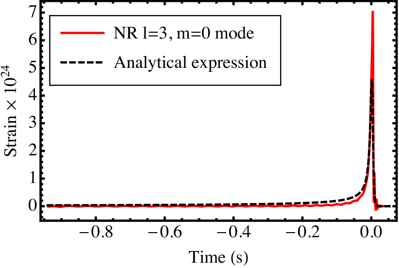
Figure 1: Spin memory mode in a numerical relativity simulation (solid red curve) and that computed from the analytical expression involving the $l=2$, $m=\pm 2$ modes (black dashed curve). The waveform is scaled to have parameters like that of the GW150914 event, which are described in greater detail in the text.

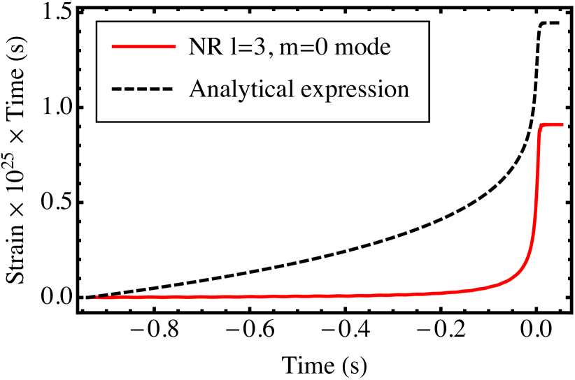
Figure 2: The spin memory effect computed directly from a numerical relativity simulation and the analytical expression containing the $l=2$, $m=\pm 2$ by integrating the curves in Fig. 1 numerically.

As a brief exercise in relating analytical and numerical-relativity predictions, we compare the spin memory mode from the simulation SXS:BBH:0305 from the SXS waveform catalog SXS with the analytical result that is given in Eq. (47). We also compare the $u$ integral of (47) and the numerical $l=3$, $m=0$ mode. It is not a strict analytical comparison in the sense that we use the $l=2$, $m=\pm 2$ modes from the numerical simulation in our analytical expression for the spin memory modes; instead, it can be thought of as a consistency check of the numerical modes with the analytical expectations for these modes.

One might be concerned that this is a fruitless exercise, because one of the major caveats noted in SXS is that the $m=0$ modes are not captured well by the extrapolation method used to compute the waveforms at future null infinity. For the displacement memory mode ($l=2$, $m=0$), the waveform computed from Eq. (48) and the $l=2$, $m=0$ mode from the simulation show large discrepancies between the two (not even qualitative similarities).

Interestingly, the spin memory modes are much more similar. For illustrative purposes, we rescale the numerical waveforms to have the same total mass, luminosity distance, and inclination as GW150914 (as detailed in Sec. V). The result of this comparison is shown in Fig. 1. The solid red curve is the numerical-relativity waveform, and the dashed black curve is the result calculated using the numerical $l=2$, $m=\pm 2$ modes and the analytical expression (47). The peak of the magnitude of the $l=2$, $m=2$ mode is chosen to be the time $t=0$ in Figs. 1 and 2. The agreement between the two methods is remarkably good, especially considering how poor it is for the displacement memory mode. We speculate that it might occur because of the nonhereditary nature of the spin memory mode or because of the higher PN order of the effect. It would be interesting to investigate this in greater detail.

To temper any overexuberance about the strength of the agreement, we also show the spin memory in Fig. 2, which was computed by integrating the two curves in Fig. 1 numerically. We chose the constants of integration so that both curves went to zero at the earliest time depicted in the figure. Even though the peak of the numerical-relativity curve in Fig. 1 is noticeably larger than that of the analytical curve, the analytical curve has a larger spin memory effect than the numerical one does. This occurs because the numerical curve hovers more closely to zero than the analytical curve does; as a result, the analytical expression is able to capture more of the gradual accumulation of the spin memory. And although the differences between the curves in Figs. 1 and 2 are larger in the latter than the former, the qualitative agreement in both is rather impressive.