Phase space curvature in spin-orbit coupled ultracold atom systems

Abstract

We consider a system with spin-orbit coupling and derive equations of motion which include the effects of Berry curvatures. We apply these equations to investigate the dynamics of particles with equal Rashba-Dresselhaus spin-orbit coupling in one dimension. In our derivation, the adiabatic transformation is performed first and leads to quantum Heisenberg equations of motion for momentum and position operators. These equations explicitly contain position-space, momentum-space, and phase-space Berry curvature terms. Subsequently, we perform the semiclassical approximation, and obtain the semiclassical equations of motion. Taking the low-Berry-curvature limit results in equations that can be directly compared to previous results for the motion of wavepackets. Finally, we show that in the semiclassical regime, the effective mass of the equal Rashba-Dresselhaus spin-orbit coupled system can be viewed as a direct effect of the phase-space Berry curvature.

I Introduction

The geometrical concept of curvature has found multiple applications in various branches of physics Frankel (2004), including the general theory of relativity Einstein (1915), gauge theories in particle physics Yang and Mills (1954), and most recently condensed-matter physics in the guise of Berry curvatures Xiao et al. (2010). In simple terms, position-space Berry curvature can be understood as a result of magnetization texture in real space, while momentum-space Berry curvature requires spin-orbit coupling (SOC) Xiao et al. (2010); Fujita et al. (2011). Here, SOC is understood in the broad sense, i.e., as linking the velocity to some quantized internal charcteristic of the particle.

Even though SOC arises naturally in crystals that lack an inversion center, that is not the case in ultra-cold atom systems Manchon et al. (2015). There, the coupling between the motion of each neutral atom and its hyperfine spin Stuhl et al. (2015) (or other degrees of freedom Livi et al. (2016); Wall et al. (2016)) has to be artificially engineered Dalibard et al. (2011). Recently, this field has seen considerable progress Galitski and Spielman (2013); Goldman et al. (2014); Zhai (2015), and some of the proposed spin-orbit coupling schemes have been experimentally realized. In particular, one-dimensional equal Rashba-Dresselhaus Rashba (1960); Dresselhaus (1955) SOC was implemented several years ago Lin et al. (2011a) and has received a substantial amount of attention Li et al. (2015). Furthermore, there has been promising experimental progress in engineering two-dimensional Rashba SOC Campbell and Spielman (2016); Huang et al. (2016), while three-dimensional Weyl SOC remains an active theoretical research direction Anderson et al. (2012, 2013); Dubček et al. (2015); Armaitis et al. (2017). Most of this work is concentrated on utilizing the internal states of the atom and transitions between them with no spatial dependence. However, other means, such as spatial degrees of freedom and periodic driving of the system can also be efficiently exploited for similar purposes Struck et al. (2012, 2014); Eckardt (2017). For example, it is possible to achieve strong effective magnetic field in optical lattices and thus simulate various condensed-matter Hamiltonians Struck et al. (2011); Lewenstein et al. (2012); Struck et al. (2013); Aidelsburger et al. (2013); Miyake et al. (2013); Goldman et al. (2016). According to the concept of synthetic dimensions Celi et al. (2014), internal degrees of freedom can be used to emulate additional spatial directions Celi et al. (2014); Mancini et al. (2015); Price et al. (2015a); Stuhl et al. (2015); Suszalski and Zakrzewski (2016); Anisimovas et al. (2016); Livi et al. (2016). In this context, coupling between spatial and internal degrees of freedom was demonstrated using both hyperfine Stuhl et al. (2015) and long-lived electronic Livi et al. (2016); Wall et al. (2016) states. Central to understanding all of these advances is the notion of the Berry phase Berry (1984).

Figure 1: In the absence of spin-orbit coupling both spin species ($\uparrow$ and $\downarrow$) respond to a spin-independent linear potential in the same way, since their masses are equal (left). When the spin-orbit coupling is turned on, adiabatic motion occurs in dispersion branches labelled by $+$ and $-$. The effective mass in the two branches is different, resulting in a different response to the same potential (right). This effect can be explained by the phase-space Berry curvature in the semiclassical regime (see Sec. VI for more details).

The Berry phase, as well as Berry curvatures in real and momentum spaces have been thoroughly discussed in literature in various contexts, see Xiao et al. (2010); Goldman et al. (2014) and references therein. However, up to now considerably less attention has been paid to phase-space Berry curvatures, especially outside the solid-state physics community. It was only recently realized that this phase-space Berry curvature can lead to an alternation of density of states Freimuth et al. (2013); Bamler (2016). This change in the density of states might in turn be used to detect topological objects, such as skyrmions, by a mundane electrical measurement. This turns out to be particularly relevant to solid-state materials, where both spin-orbit coupling and magnetization textures are present Hanneken et al. (2015); Hamamoto et al. (2016).

Theoretical progress concerning phase-space Berry curvature has been mostly concentrated on lattice systems in the semiclassical approximation. In an early publication Sundaram and Niu (1999), wavepacket propagation in a slowly perturbed crystal has been described using a combined Hamiltonian-Lagrangian approach. A derivation of the equations of motion using the Ehrenfest theorem without the Lagrangian formalism has been presented in Ref. Shindou and Imura (2005). A series of articles by P. Gosselin and coworkers has developed a purely Hamiltonian semiclassical treatment Gosselin et al. (2006, 2007, 2008a), and also perturbatively addressed the problem beyond the semiclassical (lowest order in the reduced Planck constant $\hbar$) approximation Gosselin et al. (2008b); Gosselin and Mohrbach (2009). In other work, quantum kinetic equations have been derived for multiband systems, taking the effects of phase-space Berry curvature into account Wong and Tserkovnyak (2011).

In this paper we approach the phase-space Berry curvature with applications in ultracold-atom systems in mind. We present two main results. First, we have derived quantum-mechanical Heisenberg equations of motion, where various Berry curvatures show up without relying on the semiclassical approximation, Eqs. (28). These equations also allow us to recover the semiclassical results of Ref. Sundaram and Niu (1999) by explicitly taking the small-curvature limit and purely within the Hamiltonian formalism. Second, we show that in the experimentally-accessible equal Rashba-Dresselhaus spin-orbit coupled system, the effective mass in the semiclassical single-minimum regime can be reinterpreted as the phase-space Berry curvature, cf. Fig. 1.

This paper is organized as follows. In Sec. II we present the problem and introduce the notation. In Sec. III we attack the general problem by performing an adiabatic approximation, which results in the Heisenberg equations of motion. To show that this treatment is also of practical interest, we then apply these results to two particular cases in Sec. IV. Namely, we derive the (quantum) equations of motion when either the position-space Berry curvature or the momentum-space Berry curvature is nonvanishing. In Sec. V, we perform the semiclassical approximation for the general problem and obtain the corresponding equations of motion with various Berry-curvature terms explicitly shown. We investigate the experimentally-relevant equal Rashba-Dresselhaus Hamiltonian in our framework in Sec. VI. Finally, Sec. VII summarizes our results and provides some directions for future work.

II Position-dependent spin-orbit coupling

Let us consider the following Hamiltonian with position-dependent spin-orbit coupling

$$H=\frac{\hbar^{2}}{2m}(\bm{k}I-\bm{A}(\bm{r}))^{2}+V(\bm{r})\,,$$ (1)

where $\bm{A}$ is a position-space vector of $2\times 2$ matrices in the spin space, $V$ is a spin-space matrix, and $I$ is the identity matrix. For concreteness and simplicity we consider (pseudo-)spin 1/2 atoms, i.e., systems with two dispersion branches. Generalization to higher-spin systems with more than two dispersion branches is straightforward and does not change the qualitative picture. Note that $\bm{A}$ and $V$ may depend on position $\bm{r}$ Su et al. (2015). Wavevector $\bm{k}$ and position $\bm{r}$ are (noncommuting) operators. We separate the spin-dependent part of the potential,

$$V(\bm{r})=\sum_{j}v^{j}(\bm{r})\sigma^{j}+v_{0}({\bm{r}})I$$ (2)

and also make the spin-dependence of the vector potential $\bm{A}$ explicit,

$$A_{j}(\bm{r})=\sum_{l}a_{j}^{l}({\bm{r}})\sigma^{l}\,,$$ (3)

where $\sigma^{j}$ are the Pauli matrices. Note that the square of the $\bm{A}$ matrix is proportional to the identity matrix. We write position-space vectors using bold font and their indices as subscripts, whereas spin-space vectors are denoted by the arrow above and their indices are written as superscripts. The matrix $\bm{A}$ may also contain a term proportional to the identity matrix. Such a term would describe the usual $U(1)$ electromagnetic field, which is beyond the scope of this paper, and we thus neglect it.

Using the matrices given in Eqs. (2) and (3), the Hamiltonian in Eq. (1) becomes

$$H= \frac{\hbar^{2}}{2m}I\sum_{i}k_{i}k_{i}+\sum_{j}\Big{(}-\frac{\hbar^{2}}{2m}\sum_{i}\{k_{i},a_{i}^{j}\}+v^{j}\Big{)}\sigma^{j}$$

$$+\Big{(}\sum_{i,j}\frac{\hbar^{2}}{2m}a_{i}^{j}a_{i}^{j}+v_{0}\Big{)}I\,,$$ (4)

where we have introduced the anticommutator $\{k_{i},a_{i}^{j}\}=k_{i}a_{i}^{j}+a_{i}^{j}k_{i}$. The Hamiltonian above contains a term of the Zeeman form, and thus it is natural to introduce the operator

$$B^{j}=-\frac{\hbar^{2}}{2m}\sum_{i}\{k_{i},a_{i}^{j}\}+v^{j}\,,$$ (5)

which plays the role of the magnetic field in this term. We will therefore use the term “effective magnetic field” to describe the operator $B^{j}$ from here on. Furthermore, there is a spin-independent potential in the Hamiltonian,

$$W(\bm{r})=\frac{\hbar^{2}}{2m}\sum_{i,j}[a_{i}^{j}(\bm{r})]^{2}+v_{0}(\bm{r})\,.$$ (6)

We now are in the position to write down the initial Hamiltonian in the following concise manner,

$$H=\frac{\hbar^{2}}{2m}{\bm{k}}^{2}I+\vec{B}\cdot\vec{\sigma}+W(\bm{r})I$$ (7)

We proceed to look for the solution of the time-dependent Schrödinger equation

$$i\hbar\frac{\partial}{\partial t}\Psi=H\Psi$$ (8)

using adiabatic approximation by assuming that the distance between the eigenvalues of the operator $\vec{B}\cdot\vec{\sigma}$ is large compared to the off-diagonal terms.

III General equations for adiabatic approximation

In this Section we treat the quantum mechanical problem exactly first, and then in adiabatic approximation. We do not directly perform, for example, the expansion in orders of $\hbar$ as carried out in Refs. Gosselin et al. (2006, 2007, 2008a, 2008b); Gosselin and Mohrbach (2009). Instead, we postpone the semiclassical approximation to Sec. V of the paper.

III.1 Unitary transformation

Anticipating adiabatic approximation, let us define a unitary operator $U$, which diagonalizes the term $\vec{B}\cdot\vec{\sigma}$ in spin space. Our problem is divided up into two dispersion branches which we label with the sign of the eigenvalue of the operator $\vec{B}\cdot\vec{\sigma}$. In particular, the definition of $U$ implies that

$$\mathcal{P}_{+}^{{\dagger}}{U}^{{\dagger}}\vec{B}\cdot\vec{\sigma}U\mathcal{P}_{-}=\mathcal{P}_{-}^{{\dagger}}{U}^{{\dagger}}\vec{B}\cdot\vec{\sigma}U\mathcal{P}_{+}=0\,,$$ (9)

where

$$\mathcal{P}_{+}=\left(\begin{array}[]{c}1\\ 0\end{array}\right)\,,\qquad\mathcal{P}_{-}=\left(\begin{array}[]{c}0\\ 1\end{array}\right)\,,$$ (10)

are the respective $\sigma^{z}$ eigenstates. Therefore, we can rewrite the diagonalized Zeeman term as

$${U}^{{\dagger}}\vec{B}\cdot\vec{\sigma}U=\mathcal{P}_{+}^{{\dagger}}{U}^{{\dagger}}\vec{B}\cdot\vec{\sigma}{U}\mathcal{P}_{+}+\mathcal{P}_{-}^{{\dagger}}{U}^{{\dagger}}\vec{B}\cdot\vec{\sigma}{U}\mathcal{P}_{-}\,.$$ (11)

The wavefunction in the diagonal basis is related to the original wavefunction by the same transformation,

$$\tilde{\Psi}={U}^{{\dagger}}\Psi\,.$$ (12)

Plugging this definition into Eq. (8) yields the Schrödinger equation in the new basis,

$$i\hbar\frac{\partial}{\partial t}\tilde{\Psi}=\tilde{H}\tilde{\Psi}\,,$$ (13)

where from

$$\tilde{H}={U}^{{\dagger}}H{U}$$ (14)

we see that the Hamiltonian after the transformation retains its original form,

$$\tilde{H}=\frac{\hbar^{2}}{2m}\tilde{{\bm{k}}}^{2}I+\vec{\tilde{B}}\cdot\vec{\tilde{\sigma}}+W(\tilde{{\bm{r}}})I$$ (15)

and the effect of this transformation can be incorporated through a redefinition of the effective magnetic field, position, momentum, and spin operators, namely,

$$\tilde{\bm{r}} =U^{\dagger}\bm{r}U\,,$$ (16a)

$$\tilde{\bm{k}} =U^{\dagger}\bm{k}U\,,$$ (16b)

$$\vec{\tilde{\sigma}} =U^{\dagger}\vec{\sigma}U\,.$$ (16c)

We note that though $\vec{\tilde{B}}\cdot\vec{\tilde{\sigma}}$ is proportional to $\sigma_{z}$, in general both $\vec{\tilde{B}}$ and $\vec{\tilde{\sigma}}$ have components in all three directions, and only their scalar product is diagonal in spin space.

III.2 Adiabatic approximation

Thus far our discussion has been exact. Let us now perform adiabatic approximation by assuming that the wavefunction $\tilde{\Psi}$ remains in the eigenspace of the projection operator $\mathcal{P}_{\pm}\mathcal{P}_{\pm}^{{\dagger}}$, i.e., either in the lower or the upper dispersion branch with respect to the position- and momentum-dependent effective magnetic field. Explicitly, $\tilde{\Psi}=\psi\mathcal{P}_{\pm}$ defines another wavefunction $\psi$, the components of which now evolve according to the Schrödinger equation with an effective Hamiltonian

$$H_{\mathrm{eff}}=\mathcal{P}_{\pm}^{{\dagger}}\tilde{H}\mathcal{P}_{\pm}$$ (17)

either in the lower ($-$) or the upper ($+$) branch. In the effective Hamiltonian the operators

$${\bm{r}}_{\mathrm{c}} =\mathcal{P}_{\pm}^{{\dagger}}\tilde{\bm{r}}\mathcal{P}_{\pm}=\mathcal{P}_{\pm}^{{\dagger}}{U}^{{\dagger}}{\bm{r}}{U}\mathcal{P}_{\pm}\,,$$ (18a)

$${\bm{k}}_{\mathrm{c}} =\mathcal{P}_{\pm}^{{\dagger}}\tilde{\bm{k}}\mathcal{P}_{\pm}=\mathcal{P}_{\pm}^{{\dagger}}{U}^{{\dagger}}{{\bm{k}}}{U}\mathcal{P}_{\pm}\,,$$ (18b)

appear. They describe the position and momentum operators adiabatically projected to one of the branches. These operators $\bm{r}_{\mathrm{c}}$ and $\bm{k}_{\mathrm{c}}$ are sometimes called the covariant operators Gosselin et al. (2006). They are manifestly different from their canonical counterparts, signalling breakdown of the Galilean invariance Zhang et al. (2016). Note that even though $\bm{r}_{\mathrm{c}}$ can be understood as a physical position operator (i.e., the position operator describing, e.g., the motion of the center of a wavepacket), $\bm{k}_{\mathrm{c}}$ does not correspond to kinetic momentum. A kinetic momentum, also known as physical momentum Zhang et al. (2016), operator could be obtained by performing the transformations described here on $\hbar(\bm{k}I-\bm{A})$, which is a matrix in spin space, as opposed to merely $\hbar\bm{k}$. One can convince oneself that $\hbar(\bm{k}I-\bm{A})$ is the kinetic momentum by computing the commutator between $\bm{r}_{\mathrm{c}}$ and the Hamiltonian in Eq. (1).

Since the position operator $\bm{r}$ and the momentum operator $\hbar\bm{k}$ are both spin independent, the projection operator commutes with them. Using this property, the last two equations can be rewritten as

$$\bm{r}_{\mathrm{c}} =\bm{r}-\bm{\mathcal{A}}^{(k)}\,,$$ (19a)

$$\bm{k}_{\mathrm{c}} =\bm{k}-\bm{\mathcal{A}}^{(r)}\,,$$ (19b)

where

$$\bm{\mathcal{A}}^{(k)} =-\mathcal{P}_{\pm}^{{\dagger}}{U}^{{\dagger}}[{\bm{r}},{U}]\mathcal{P}_{\pm}\,,$$ (20a)

$$\bm{\mathcal{A}}^{(r)} =-\mathcal{P}_{\pm}^{{\dagger}}{U}^{{\dagger}}[{{\bm{k}}},{U}]\mathcal{P}_{\pm}\,.$$ (20b)

Operators $\bm{\mathcal{A}}^{(k)}$ and $\bm{\mathcal{A}}^{(r)}$ represent the Berry connections. Given a suitable representation, commutators in these operators become derivatives, e.g., a commutator of a function with the position operator is proportional to a momentum derivative in the momentum representation. Therefore, when the operator $U$ is diagonal in position or momentum basis, the Berry connection operator $\bm{\mathcal{A}}^{(k)}$ or $\bm{\mathcal{A}}^{(r)}$ becomes a connection in the usual geometric sense, see Eqs. (30) and (39) below. This also explains the seemingly counter-intuitive labeling, which is standard Xiao et al. (2010).

In order to evaluate the potential term it is beneficial to expand $W({\bm{r}})$ in a power series,

$$W({\bm{r}})=w^{(0)}+\sum_{j}w_{j}^{(1)}r_{j}+\sum_{j,l}w_{jl}^{(2)}r_{j}r_{l}+\cdots\,.$$ (21)

In most ultracold-atom-related problems the potential $W$ is at most quadratic, and we will therefore limit our attention to such cases. Cubic and higher order terms in the potential $W$ would result in a more complicated expression in Eq. (24b). The effective Hamiltonian $H_{\mathrm{eff}}$ can thus be rewritten in the following concise form:

$$H_{\mathrm{eff}}=\frac{\hbar^{2}}{2m}{\bm{k}}_{\mathrm{c}}^{2}+W({\bm{r}}_{\mathrm{c}})+\mathcal{V}\,,$$ (22)

where

$$\mathcal{V}=\mathcal{P}_{\pm}^{{\dagger}}\vec{\tilde{B}}\cdot\vec{\tilde{\sigma}}\mathcal{P}_{\pm}+\mathcal{V}^{(r)}+\mathcal{V}^{(k)}\,,$$ (23)

with

$$\mathcal{V}^{(r)} =\frac{\hbar^{2}}{2m}\big{(}\mathcal{P}_{\pm}^{{\dagger}}{U}^{{\dagger}}[{{\bm{k}}},{U}]\mathcal{P}_{\mp}\big{)}\cdot\big{(}\mathcal{P}_{\mp}^{{\dagger}}{U}^{{\dagger}}[{{\bm{k}}},{U}]\mathcal{P}_{\pm}\big{)}\,,$$ (24a)

$$\mathcal{V}^{(k)} =\sum_{j,l}w_{jl}^{(2)}\mathcal{P}_{\pm}^{{\dagger}}{U}^{{\dagger}}[r_{j},{U}]\mathcal{P}_{\mp}\mathcal{P}_{\mp}^{{\dagger}}{U}^{{\dagger}}[r_{l},{U}]\mathcal{P}_{\pm}\,.$$ (24b)

We see that besides the alternation of the physical momentum and position operators, three extra potential terms have appeared. In the following subsections we investigate dynamics in this system in more detail.

III.3 Heisenberg equations

As discussed above, the operators ${\bm{r}}_{\mathrm{c}}$ and $\hbar{\bm{k}}_{\mathrm{c}}$ do not represent the canonical position and momentum. This is confirmed by the observation that their commutators differ from the usual commutators for the position and momentum operators. In particular, not only the position-momentum commutator gains an extra term, but the other commutators do not vanish anymore:

$$[(r_{\mathrm{c}})_{j},(r_{\mathrm{c}})_{l}] =i\Theta_{jl}^{(k,k)}\,,$$ (25a)

$$[(k_{\mathrm{c}})_{j},(k_{\mathrm{c}})_{l}] =i\Theta_{jl}^{(r,r)}\,,$$ (25b)

$$[(r_{\mathrm{c}})_{j},(k_{\mathrm{c}})_{l}] =i\delta_{j,l}+i\Theta_{jl}^{(k,r)}\,,$$ (25c)

where various Berry curvatures are given by

$$\Theta_{jl}^{(k,k)} =i[r_{j},\mathcal{A}_{l}^{(k)}]-i[r_{l},\mathcal{A}_{j}^{(k)}]\,,$$ (26a)

$$\Theta_{jl}^{(r,r)} =i[{k}_{j},\mathcal{A}_{l}^{(r)}]-i[{k}_{l},\mathcal{A}_{j}^{(r)}]\,,$$ (26b)

$$\Theta_{jl}^{(k,r)} =i[r_{j},\mathcal{A}_{l}^{(r)}]-i[{k}_{l},\mathcal{A}_{j}^{(k)}]\,,$$ (26c)

$$\Theta_{jl}^{(r,k)} =i[{k}_{j},\mathcal{A}_{l}^{(k)}]-i[r_{l},\mathcal{A}_{j}^{(r)}]\,,$$ (26d)

and also note that $\Theta_{jl}^{(k,r)}=-\Theta_{lj}^{(r,k)}$. The emergence of the extra terms in Eqs. (25) can be interpreted as curving up of position space, momentum space, and phase space, respectively. In quantum mechanics phase space is inherently curved, as position and momentum operators do not commute to begin with. Eqs. (25) demonstrate that non-commutative geometry underlies the algebraic structure of coordinates and momenta. Non-commutative coordinates in the context of field theory, and physics in general, have attracted a great deal of theoretical interest Seiberg and Witten (1999); Douglas and Nekrasov (2001).

Adiabatic approximation, and spin projection in particular, is essential to obtaining a nonzero Berry curvature (see Ref. Fujita et al. (2011) for an extensive discussion). If no spin projection is performed, Berry connections generally have a nontrivial matrix structure. Schematically, this matrix structure serves to generate terms of the $[\mathcal{A},\mathcal{A}]$ type, which exactly cancel the corresponding $[k,\mathcal{A}]$ and $[r,\mathcal{A}]$ terms. In this way it is ensured that a change of basis in spin space leaves physical dynamics unchanged. On the other hand, adiabatic approximation confines evolution of the system to only one of the two dispersion branches, and the price for that simplification is the emergence of Berry curvature.

Going beyond adiabatic approximation would bring about effects similar to Zitterbewegung, see Refs. Merkl et al. (2008); LeBlanc et al. (2013); Winkler et al. (2007). In that case, noncommuting components of the velocity operator $\dot{\bm{r}}_{\mathrm{c}}$ signal interbranch transitions. The frequency of these transitions is given by the gap between the dispersion branches.

Naturally, modified commutation relations result in altered Heisenberg equations for the covariant operators

$$\dot{\bm{k}}_{\mathrm{c}} =\frac{1}{i\hbar}[{\bm{k}}_{\mathrm{c}},H_{\mathrm{eff}}]\,,$$ (27a)

$$\dot{\bm{r}}_{\mathrm{c}} =\frac{1}{i\hbar}[{\bm{r}}_{\mathrm{c}},H_{\mathrm{eff}}]\,,$$ (27b)

which now contain the Berry curvature terms defined above,

$$\dot{\bm{k}}_{\mathrm{c}}= -\frac{1}{\hbar}\bm{\nabla}W({\bm{r}}_{\mathrm{c}})+\frac{1}{i\hbar}[{\bm{k}}_{\mathrm{c}},\mathcal{V}]$$ (28a)

$$+\frac{\hbar}{2m}\sum_{j,l}\bm{e}_{j}\{\Theta_{jl}^{(r,r)},(k_{\mathrm{c}})_{l}\}$$

$$+\frac{1}{2\hbar}\sum_{j,l}\bm{e}_{j}\{\Theta_{jl}^{(r,k)},\nabla_{l}W(\bm{r}_{\mathrm{c}})\}\,,$$

$$\dot{\bm{r}}_{\mathrm{c}}= \frac{\hbar}{m}{\bm{k}}_{\mathrm{c}}+\frac{1}{i\hbar}[{\bm{r}}_{\mathrm{c}},\mathcal{V}]$$ (28b)

$$+\frac{\hbar}{2m}\sum_{j,l}\bm{e}_{j}\{\Theta_{jl}^{(k,r)},(k_{\mathrm{c}})_{l}\}$$

$$+\frac{1}{2\hbar}\sum_{j,l}\bm{e}_{j}\{\Theta_{jl}^{(k,k)},\nabla_{l}W(\bm{r}_{\mathrm{c}})\}\,,$$

where $\bm{e}_{j}$ denotes the unit vector in the $j$ direction (i.e., $\bm{e}_{j}$ is a vector, and not a component of a vector), while all the $\nabla$’s here act on functions of a single variable, and thus represent derivatives with respect to that variable. This set of Eqs. (28) represents the first main result of the paper.

The first term on the right-hand side in each of the two equations denotes the usual contribution known from classical mechanics, whereas the subsequent terms are due to adiabatic approximation. In particular, in each case the second term is due to emergent potentials, whereas the last two terms are due to Berry curvatures. In order to make our hitherto abstract discussion more concrete, we consider two simple examples next.

IV Particular cases

Let us consider the situation where the operator $\vec{B}$ becomes a vector of complex numbers (as opposed to operators) in some representation. In this case the eigenvalues of the operator $\vec{B}\cdot\vec{\sigma}$ are $\pm|\vec{B}|$ with the eigenfunctions

$$\chi_{+}=\left(\begin{array}[]{c}e^{-i\frac{\phi}{2}}\cos\frac{\alpha}{2}\\ e^{i\frac{\phi}{2}}\sin\frac{\alpha}{2}\end{array}\right)\,,\quad\chi_{-}=\left(\begin{array}[]{c}e^{-i\frac{\phi}{2}}\sin\frac{\alpha}{2}\\ -e^{i\frac{\phi}{2}}\cos\frac{\alpha}{2}\end{array}\right)\,,$$ (29)

where the spherical angles $\alpha$ and $\phi$ give the direction of the vector $\vec{B}$. The unitary operator ${U}$, which diagonalizes the matrix $\vec{B}\cdot\vec{\sigma}$, then consists of two columns, $\chi_{+}$ and $\chi_{-}$. Two particular cases, which often occur in practice, are a position-dependent effective magnetic field, and spin-orbit coupling which corresponds to a momentum-dependent Zeeman term. We investigate them in more detail below.

IV.1 Position space curvature

When the operator $\vec{B}$ depends only on the coordinate $\bm{r}$, the unitary transformation operator is a function of position only: $U=U(\bm{r})$. In this case the Berry connections are $\bm{\mathcal{A}}^{(k)}=0$ and

$$\bm{\mathcal{A}}^{(r)}=i\chi_{\pm}^{{\dagger}}(\bm{r})\bm{\nabla}^{(r)}\chi_{\pm}(\bm{r})\,.$$ (30)

The corresponding Berry curvatures are $\Theta^{(k,k)}=\Theta^{(k,r)}=\Theta^{(r,k)}=0$ and

$$\Theta_{jl}^{(r,r)}=\nabla_{j}^{(r)}\mathcal{A}_{l}^{(r)}-\nabla_{l}^{(r)}\mathcal{A}_{j}^{(r)}\,.$$ (31)

The scalar potentials are $\mathcal{V}^{(k)}=0$ and

$$\mathcal{V}^{(r)}=-\frac{\hbar^{2}}{2m}\left(\chi_{\pm}^{{\dagger}}\bm{\nabla}^{(r)}\chi_{\mp}\right)\cdot\left(\chi_{\mp}^{{\dagger}}\bm{\nabla}^{(r)}\chi_{\pm}\right)\,.$$ (32)

These quantities can also be expressed in terms of the angles on the Bloch sphere, namely, $\alpha$ and $\phi$. Concretely, the Berry connection is

$$\bm{\mathcal{A}}^{(r)}=\pm\frac{1}{2}\cos\alpha\bm{\nabla}^{(r)}\phi\,,$$ (33)

the potential is the same for the two branches,

$$\mathcal{V}^{(r)}=\frac{\hbar^{2}}{8m}\Big{(}(\bm{\nabla}^{(r)}\alpha)^{2}+\sin^{2}\alpha(\bm{\nabla}^{(r)}\phi)^{2}\Big{)}\,,$$ (34)

while the Berry curvature is opposite for the two brances,

$$\Theta^{(r,r)}_{jl}= \pm\frac{\sin\alpha}{2}\Big{(}(\nabla^{(r)}_{j}\phi)(\nabla^{(r)}_{l}\alpha)$$

$$-(\nabla^{(r)}_{j}\alpha)(\nabla^{(r)}_{l}\phi)\Big{)}\,.$$ (35)

The latter two equations can also be conveniently expressed using the unit vector $\vec{n}=\vec{B}/|\vec{B}|$, describing the direction of the vector $\vec{B}$ Volovik (1987),

$$\mathcal{V}^{(r)} =\frac{\hbar^{2}}{8m}(\bm{\nabla}^{(r)}\vec{n})^{2}\,,$$ (36)

$$\Theta^{(r,r)}_{jl} =\mp\frac{1}{2}\vec{n}\cdot(\nabla_{j}^{(r)}\vec{n}\times\nabla_{l}^{(r)}\vec{n})\,.$$ (37)

The equations of motion (28) in this case are

$$\dot{\bm{k}}_{\mathrm{c}}= -\frac{1}{\hbar}\bm{\nabla}^{(r)}W({\bm{r}}_{\mathrm{c}})+\frac{1}{i\hbar}[{\bm{k}}_{\mathrm{c}},\mathcal{V}]$$ (38a)

$$+\frac{\hbar}{2m}\sum_{j,l}\bm{e}_{j}\{\Theta_{jl}^{(r,r)},(k_{\mathrm{c}})_{l}\}\,,$$

$$\dot{\bm{r}}_{\mathrm{c}}= \frac{\hbar}{m}{\bm{k}}_{\mathrm{c}}\,.$$ (38b)

The curvature $\Theta_{jl}^{(r,r)}$ is also known as the synthetic magnetic field and has been studied theoretically Dalibard et al. (2011); Goldman et al. (2014) as well as experimentally Lin et al. (2009); Beeler et al. (2013). Note that the Stern-Gerlach experiment Gerlach and Stern (1922), which is often discussed in introductory quantum mechanics textbooks Sakurai (1994), can also be described in this framework. In particular, a linear magnetic field gradient separates out the two spin components since the Berry connection in position space becomes nonzero, even though the Berry curvature itself vanishes in that case.

IV.2 Momentum space curvature

When operator $\vec{B}$ depends only on momentum $\bm{k}$, basis transformation is facilitated by $U=U(\bm{k})$, which then is a function of momentum only. In this case, the position-space Berry connection vanishes, $\bm{\mathcal{A}}^{(r)}=0$, whereas

$$\boldsymbol{\mathcal{A}}^{(k)}=-i\chi_{\pm}^{{\dagger}}\bm{\nabla}^{(k)}\chi_{\pm}\,.$$ (39)

Accordingly, the Berry curvature components related to position space vanish, $\Theta^{(r,r)}=\Theta^{(k,r)}=\Theta^{(r,k)}=0$, and all the curvature is concentrated in the momentum space,

$$\Theta_{jl}^{(k,k)}=-\nabla_{j}^{(k)}\mathcal{A}_{l}^{(k)}+\nabla_{l}^{(k)}\mathcal{A}_{j}^{(k)}\,.$$ (40)

The scalar potential has momentum components only, i.e., $\mathcal{V}^{(r)}=0$ and

$$\mathcal{V}^{(k)}=-\sum_{j,l}w_{jl}^{(2)}\left(\chi_{\pm}^{{\dagger}}\nabla^{(k)}_{j}\chi_{\mp}\right)\left(\chi_{\mp}^{{\dagger}}\nabla^{(k)}_{l}\chi_{\pm}\right)\,.$$ (41)

Equations similar to Eqs. (34) – (37) can also be written down in the case at hand. Finally, Heisenberg equations of motion (28) in this case are

$$\dot{\bm{k}}_{\mathrm{c}}= -\frac{1}{\hbar}\bm{\nabla}^{(r)}W({\bm{r}}_{\mathrm{c}})\,,$$ (42a)

$$\dot{\bm{r}}_{\mathrm{c}}= \frac{\hbar}{m}{\bm{k}}_{\mathrm{c}}+\frac{1}{i\hbar}[{\bm{r}}_{\mathrm{c}},\mathcal{V}]$$ (42b)

$$+\frac{1}{2\hbar}\sum_{j,l}\bm{e}_{j}\{\Theta_{jl}^{(k,k)},\nabla^{(r)}_{l}W(\bm{r}_{\mathrm{c}})\}\,.$$

We remark that strictly speaking when the two dispersion branches touch, adiabatic approximation becomes invalid. The condition for the validity of adiabatic approximation is particularly elegant in this momentum-space curvature case. Concretely, $|\vec{B}|$ must be nonzero for each $\bm{k}$. This only is the case when the system of equations

$$-\frac{\hbar^{2}}{m}\sum_{i}k_{i}a_{i}^{j}+v^{j}=0$$ (43)

has no solutions. In terms of $\bm{k}$, this system of equations is linear. Therefore, the branches do not touch only if the following determinant in spin space vanishes:

$$\sum_{j,l,n}\epsilon^{jln}a_{1}^{j}a_{2}^{l}a_{3}^{n}=0,$$ (44)

where $\epsilon^{jln}$ is the Levi-Civita symbol. Effects of the momentum-space curvature have already been extensively studied theoretically Price et al. (2014, 2015b).

V Semiclassical approximation

As we have seen in the last section, in cases where all the Berry curvature is concentrated in a single component, for example, as either position-space curvature or momentum-space curvature, the equations of motion are relatively simple and can often be treated exactly. However, this is not the case in general. Moreover, in the definition of the Berry connection or the Berry curvatures, $\hbar$ is crucially absent, suggesting that these quantities also affect semiclassical dynamics. Finally, semiclassical approximation is of practical interest, as it allows one to investigate the motion of wavepackets and clouds of ultracold atoms in particular. Motivated by these points, we consider semiclassical approximation in general in this Section, and proceed to apply it to particular Hamiltonians subsequently.

In semiclassical approximation we neglect the commutator between position and momentum. In that case the effective magnetic field operator becomes

$$B^{j}=-\frac{\hbar^{2}}{m}\sum_{i}k_{i}a_{i}^{j}(\bm{r})+v^{j}(\bm{r})\,.$$ (45)

The matrix $\vec{B}\cdot\vec{\sigma}$ still has the eigenvectors $\chi_{\pm}$, but they now parametrically depend on the numbers $\bm{r}$ and $\bm{k}$. Berry connections (20) are

$$\bm{\mathcal{A}}^{(r)} =i\chi_{\pm}^{\dagger}\bm{\nabla}^{(r)}\chi_{\pm}\,,$$ (46a)

$$\bm{\mathcal{A}}^{(k)} =-i\chi_{\pm}^{\dagger}\bm{\nabla}^{(k)}\chi_{\pm}\,,$$ (46b)

and lead to corresponding Berry curvatures (26)

$$\Theta_{jl}^{(k,k)} =-\nabla^{(k)}_{j}\mathcal{A}_{l}^{(k)}+\nabla^{(k)}_{l}\mathcal{A}_{j}^{(k)}\,,$$ (47a)

$$\Theta_{jl}^{(r,r)} =\nabla^{(r)}_{j}\mathcal{A}_{l}^{(r)}-\nabla^{(r)}_{l}\mathcal{A}_{j}^{(r)}\,,$$ (47b)

$$\Theta_{jl}^{(k,r)} =-\nabla^{(k)}_{j}\mathcal{A}_{l}^{(k)}-\nabla^{(r)}_{l}\mathcal{A}_{j}^{(r)}\,,$$ (47c)

$$\Theta_{jl}^{(r,k)} =\nabla^{(r)}_{j}\mathcal{A}_{l}^{(r)}+\nabla^{(k)}_{l}\mathcal{A}_{j}^{(k)}\,,$$ (47d)

and scalar potentials (24)

$$\mathcal{V}^{(r)} =-\frac{\hbar^{2}}{2m}\left(\chi_{\pm}^{{\dagger}}\bm{\nabla}^{(r)}\chi_{\mp}\right)\cdot\left(\chi_{\mp}^{{\dagger}}\bm{\nabla}^{(r)}\chi_{\pm}\right)\,,$$ (48a)

$$\mathcal{V}^{(k)} =-\sum_{j,l}w_{jl}^{(2)}\chi_{\pm}^{{\dagger}}\nabla^{(k)}_{j}\chi_{\mp}\chi_{\mp}^{{\dagger}}\nabla^{(k)}_{l}\chi_{\pm}\,.$$ (48b)

Equations of motion (28) then take the form

$$\dot{\bm{k}}_{\mathrm{c}}= -\frac{1}{\hbar}\bm{\nabla}^{(r)}W-\frac{1}{\hbar}\bm{\nabla}^{(r)}\mathcal{V}$$ (49a)

$$+\frac{\hbar}{m}\sum_{j,l}\bm{e}_{j}\Theta_{jl}^{(r,r)}(k_{\mathrm{c}})_{l}$$

$$+\frac{1}{\hbar}\sum_{j,l}\bm{e}_{j}\Theta_{jl}^{(r,k)}\nabla^{(r)}_{l}W\,,$$

$$\dot{\bm{r}}_{\mathrm{c}}= \frac{\hbar}{m}{\bm{k}}_{\mathrm{c}}+\frac{1}{\hbar}\bm{\nabla}^{(k)}\mathcal{V}$$ (49b)

$$+\frac{\hbar}{m}\sum_{j,l}\bm{e}_{j}\Theta_{jl}^{(k,r)}(k_{\mathrm{c}})_{l}$$

$$+\frac{1}{\hbar}\sum_{j,l}\bm{e}_{j}\Theta_{jl}^{(k,k)}\nabla^{(r)}_{l}W\,.$$

We see that in semiclassical approximation Berry curvatures $\Theta$ and scalar potentials $\mathcal{V}$ do not vanish and still show up in the equations of motion. However, since they involve derivatives of the eigenvectors $\chi_{\pm}$, which vary at scales much larger than the other relevant length scales, e.g., the de Broglie wavelength, these quantities are not dominant. Therefore, it is a reasonable approximation to insert classical relations $\dot{\bm{k}}_{\mathrm{c}}\approx-\bm{\nabla}^{(r)}W/\hbar$ and $\dot{\bm{r}}_{\mathrm{c}}\approx{\hbar}{\bm{k}}_{\mathrm{c}}/m$ on the right-hand side of the equations of motion. In that case, we arrive at

$$\dot{\bm{k}}_{\mathrm{c}}= -\frac{1}{\hbar}\bm{\nabla}^{(r)}(W+\mathcal{V})$$ (50a)

$$+\sum_{j,l}\bm{e}_{j}\left(\Theta_{jl}^{(r,r)}(\dot{r}_{\mathrm{c}})_{l}+\Theta_{lj}^{(k,r)}(\dot{k}_{\mathrm{c}})_{l}\right)\,,$$

$$\dot{\bm{r}}_{\mathrm{c}}= \frac{\hbar}{m}{\bm{k}}_{\mathrm{c}}+\frac{1}{\hbar}\bm{\nabla}^{(k)}\mathcal{V}$$ (50b)

$$-\sum_{j,l}\bm{e}_{j}\left(\Theta_{lj}^{(r,k)}(\dot{r}_{\mathrm{c}})_{l}+\Theta_{jl}^{(k,k)}(\dot{k}_{\mathrm{c}})_{l}\right)\,,$$

where we have grouped the terms in order to facilitate comparison with Eqs. (2.19) in Ref. Sundaram and Niu (1999). Even though the result is the same, we arrived at it purely within the Hamiltonian formalism. Furthermore, in our derivation we have shown that these equations constitute a special case of the semiclassical situation, namely, they are only valid when Berry curvatures are small.

VI One-dimensional spiral

Up to this point our discussion was valid for an arbitrary number of spatial dimensions. Now we specialize to a single spatial dimension, where the effects of phase space Berry curvature are nevertheless nontrivial, as phase space in this case is two dimensional. In particular, as an application of the discussion above, in this Section we investigate the dynamics described by the following one-dimensional Hamiltonian:

$$H=H_{0}-FxI\,,$$ (51)

where the $-FxI$ term describes a spin-independent force (linear potential), while

$$H_{0}= \frac{\hbar^{2}}{2m}(kI-a\sigma_{3})^{2}$$ (52)

$$+\frac{\hbar\Omega}{2}\Big{(}\cos\frac{x}{\lambda}\,\sigma_{1}+\sin\frac{x}{\lambda}\,\sigma_{2}\Big{)}$$

is an exactly-solvable Hamiltonian with a constant spin-orbit coupling term and a position-dependent Zeeman term. The spin-orbit coupling term is characterized by its constant strength $a$. The position-space Zeeman term constitutes a spiral with a constant magnitude $\Omega/2$ and a wavelength $\lambda$. Furthermore, it is convenient to introduce the wavenumber

$$\kappa=\frac{\Omega}{2a}\frac{m}{\hbar}\,,$$ (53)

which quantifies the relative strength of the position-space and momentum-space Zeeman terms. This Hamiltonian $H_{0}$ is well known: it has undergone an extensive theoretical investigation (see Ref. Li et al. (2015) and references therein) and has also been realized experimentally Lin et al. (2011a).

VI.1 Exact solution

In this subsection we recap the exact diagonalization Li et al. (2015) of $H_{0}$. We begin by observing that the Zeeman term can be rewritten as

$$\cos(x/\lambda)\sigma_{1}+\sin(x/\lambda)\sigma_{2}=e^{-i\frac{x}{2\lambda}\sigma_{3}}\sigma_{1}e^{i\frac{x}{2\lambda}\sigma_{3}}\,,$$ (54)

and hence the coordinate dependence may be eliminated by performing a unitary transformation. Concretely, the wave function in the new basis is

$$\tilde{\Psi}=U^{{\dagger}}\Psi\,,$$ (55)

where

$$U=e^{-i\frac{x}{2\lambda}\sigma_{3}}\,.$$ (56)

We then obtain the transformed Hamiltonian

$$\tilde{H}_{0}=U^{{\dagger}}H_{0}U=\frac{\hbar^{2}}{2m}(k-k_{0}\sigma_{3})^{2}+\frac{\hbar\Omega}{2}\sigma_{1}\,,$$ (57)

where

$$k_{0}=a+\frac{1}{2\lambda}\,.$$ (58)

The symbols in this Hamiltonian directly correspond to physical quantities in the experimental realization of the model Lin et al. (2011a); Li et al. (2015). In particular, given two lasers with small detuning from the Raman resonance, $k_{0}$ is the wavevector difference of the lasers (recoil wavevector), and $E_{R}=\hbar^{2}k_{0}^{2}/2m$ is the recoil energy. The intensity of the two lasers is represented by the Rabi frequency $\Omega$. The dispersion is thus given by

$$\frac{E}{\hbar^{2}/m}=\frac{k^{2}}{2}+\frac{k_{0}^{2}}{2}\pm\sqrt{(kk_{0})^{2}+\frac{\Omega^{2}}{4}\left(\frac{m}{\hbar}\right)^{2}}$$ (59)

in the lower ($-$) and the upper ($+$) branch. The upper branch has a single quadratic minimum, wheras the lower branch has one quadratic minimum when

$$\hbar\Omega>4E_{R}\,,$$ (60)

and two quadratic minima or one quartic minimum otherwise. As the gap between the two branches is governed by the ratio $\hbar\Omega/E_{R}$, and we will be interested in the situation where the adiabatic approximation is applicable, we limit further discussion to the single minimum regime given in Eq. (60). Expanding the dispersion around the minimum $k=0$, we find that the effective mass $m^{*}_{\pm}$ in the two branches is given by

$$\frac{m}{m^{*}_{\pm}}=1\pm\frac{2k_{0}^{2}}{\Omega}\frac{\hbar}{m}\approx 1\pm\frac{1}{\kappa}\left(a+\frac{1}{\lambda}\right)\,,$$ (61)

respectively. The first equality applies in the limit $k\ll k_{0}$ of interest when computing the effective mass, whereas the second approximation holds in the semiclassical regime. Indeed, the smallness of $1/\lambda a$ and $1/\lambda\kappa$ defines the semiclassical regime, where all the gradients are small compared to the de Broglie wavelength. Namely, when the period of the spiral $\lambda$ in the position-space Zeeman term is large as compared to the spin-orbit coupling wavenumber $a$, we have $1/\lambda a\ll 1$. In combination to the single-minimum condition, this also implies $1/\lambda\kappa\ll 1$. Note further that one can transform back from the physical Hamiltonian $\tilde{H}_{0}$ in Eq. (57) to the original Hamiltonian $H_{0}$, Eq. (52), with arbitrary $\lambda$ and $a$ as long as Eq. (58) is satisfied.

In order to investigate the dynamics of the full Hamiltonian $H$, the force term $-FxI$ may be added to the exact solution as a perturbation. In that case one concludes that in the presence of spin-orbit coupling, the two branches (effective spin components) respond to a force differently, as one of them accelerates faster than the other.

VI.2 Semiclassical solution

We now treat $H$ including the effect of the force $F$ explicitly, and also carefully tracing the effects of Berry curvatures in this system. The full Zeeman term now is a position- and momentum-dependent matrix:

$$\vec{B}\cdot\vec{\sigma}=\frac{\hbar\Omega}{2}\Big{(}\cos\frac{x}{\lambda}\,\sigma_{1}+\sin\frac{x}{\lambda}\,\sigma_{2}\Big{)}-\frac{\hbar^{2}}{m}ak\sigma_{3}\,.$$ (62)

As this term contains both position and momentum operators, it does not conform to either of the cases addressed in Sec. IV. We therefore have to resort to the semiclassical approach.

The direction of the vector $\vec{B}$ can be written in terms of the spherical angles $\alpha(k)$ and $\phi(x)$ as introduced in Eq. (29). In particular,

$$\tan\alpha =-\frac{\kappa}{k}\,,$$ (63a)

$$\phi =\frac{x}{\lambda}\,.$$ (63b)

The eigenvalues of the matrix $\vec{B}\cdot\vec{\sigma}$ are

$$\pm|\vec{B}|=\pm\frac{\hbar\Omega}{2\kappa}\sqrt{\kappa^{2}+k^{2}}\,.$$ (64)

For adiabatic approximation to hold, it is sufficient that the gap between the two branches, $2|\vec{B}|$, is larger than all the other relevant energy scales. This condition in particular enforces the single-minimum condition Eq. (60). The Berry connections are $\mathcal{A}^{(k)}=0$ and

$$\mathcal{A}^{(r)}=\mp\frac{k}{2\lambda\sqrt{\kappa^{2}+k^{2}}}$$ (65)

in this case. Note that due to the nonvanishing ${\mathcal{A}}^{(r)}$, cf. Eq. (19b), the physical momentum differs from the canonical momentum,

$$k_{\mathrm{c}}=k\left(1\pm\frac{1}{2\lambda\sqrt{\kappa^{2}+k^{2}}}\right)\,.$$ (66)

Position and momentum spaces remain flat, $\Theta^{(k,k)}=\Theta^{(r,r)}=0$, and only phase-space Berry curvature is nonzero and opposite for the two branches:

$$\Theta^{(k,r)}=-\Theta^{(r,k)}=\pm\frac{\kappa^{2}}{2\lambda(\kappa^{2}+k^{2})^{\frac{3}{2}}}\,.$$ (67)

The scalar potentials (23) are $\mathcal{V}^{(k)}=0$ and

$$\mathcal{V}^{(r)}=\frac{\hbar^{2}}{8m\lambda^{2}}\frac{\kappa^{2}}{\kappa^{2}+k^{2}}\,,$$ (68)

and thus the full potential $\mathcal{V}$ is

$$\mathcal{V}=\pm\frac{\hbar\Omega}{2\kappa}\sqrt{\kappa^{2}+k^{2}}+\frac{\hbar^{2}}{8m\lambda^{2}}\frac{\kappa^{2}}{\kappa^{2}+k^{2}}\,.$$ (69)

Semiclassical dynamics follows the equations (49)

$$\dot{k}_{\mathrm{c}}= \frac{F}{\hbar}(1-\Theta^{(r,k)})\,,$$ (70a)

$$\dot{x}_{\mathrm{c}}= \frac{\hbar}{m}{k}_{\mathrm{c}}(1+\Theta^{(k,r)})+\frac{1}{\hbar}\nabla^{(k)}\mathcal{V}\,,$$ (70b)

which in general are quite complicated.

However, for our semiclassical approach to be valid, we should keep only the lowest-order corrections in the small parameters $1/\lambda a$ and $1/\lambda\kappa$. Furthermore, in order to prevent the kinetic energy from causing sizeable interbranch transitions, we limit ourselves to the $|k|\ll\kappa$ regime, where adiabatic approximation holds. These approximations lead to

$$k_{\mathrm{c}} \approx k\left(1\pm\frac{1}{2\lambda\kappa}\right)\,,$$ (71a)

$$\Theta^{(r,k)} =-\Theta^{(k,r)}\approx\mp\frac{1}{2\lambda\kappa}\,,$$ (71b)

$$\frac{1}{\hbar}\nabla^{(k)}\mathcal{V} \approx\pm\frac{k}{\kappa}\frac{\Omega}{2\kappa}\,.$$ (71c)

Therefore, equations of motion in this limit are

$$\dot{k}_{\mathrm{c}} =\frac{F}{\hbar}\left(1\pm\frac{1}{2\lambda\kappa}\right)\,,$$ (72a)

$$\dot{x}_{\mathrm{c}} =\frac{\hbar}{m}k_{\mathrm{c}}\left(1\pm\frac{1}{2\lambda\kappa}\pm\frac{a}{\kappa}\right)\,,$$ (72b)

and for the center-of-mass motion we obtain the following closed equation:

$$\ddot{x}_{\mathrm{c}}=\frac{F}{m}\left(1\pm\frac{1}{\kappa}\left(\frac{1}{\lambda}+a\right)\right)\,.$$ (73)

From this equation one can read off the effective mass, which is then seen to match the one given in Eq. (61).

We conclude that the effective mass in this model in semiclassical approximation is correctly captured for both branches by the phase-space Berry curvature. The Berry-curvature result is compared with the bare mass and also with the exact solution in Fig. 2. Thus, the effective mass measurement is a direct probe of the phase-space Berry curvature in this system. Therefore, effective-mass measurements in Refs. Lin et al. (2011b); Zhang et al. (2012) can be reinterpreted as the first measurements of phase-space Berry curvature in ultracold-atom systems. This conclusion is the second main result of the paper.

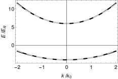
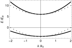
Figure 2: Dispersion of the two branches in the units of the recoil energy $E_{R}$ and the recoil wavevector $k_{0}$ in the semiclassical single-minimum regime, $\hbar\Omega/E_{R}=10$. The effective mass from the phase-space Berry-curvature in Eq. (73) (solid line) is compared to the exact result (dashed line, left) and the bare-mass approximation $m^{*}_{\pm}=m$ (dotted line, right).

VII Summary and outlook

In summary, we have presented a derivation of equations of motion in the presence of position-space, momentum-space and phase-space Berry curvatures. We have only relied on the Hamiltonian formalism, and we have clearly separated adiabatic approximation, semiclassical approximation, and the low-curvature limit. Our approach has resulted in the Heisenberg equations of motion Eqs. (28), which are written down with no reference to semiclassical approximation. From them, we have derived the semiclassical equations of motion Eqs. (49). In the limit of small curvature they reduce to Eqs. (50). The latter can be directly compared to the results of Ref. Sundaram and Niu (1999). Moreover, we have investigated the semiclassical dynamics in a system with an equal Rashba-Dresselhaus spin-orbit coupling system in a single spatial dimension. We have concluded that in the strong-coupling regime, where the dispersions of both branches are quadratic, the effective mass is directly related to phase-space Berry curvature.

Several directions of future work look promising. On the one hand, populating optical lattices with ultracold atoms one can go far beyond the regimes readily achievable in solid-state physics. In particular, it possible to engineer strong artificial magnetic fields Aidelsburger et al. (2013); Miyake et al. (2013); Aidelsburger et al. (2015) as well as strong synthetic spin-orbit coupling Livi et al. (2016); Wall et al. (2016); Kolkowitz et al. (2017), while motion of wave packets can be controlled and observed with remarkable precision Alberti et al. (2009, 2010); Haller et al. (2010). This motivates one to generalize the presented approach and revisit the effects of phase-space Berry curvature on a lattice. Furthermore, in higher-dimensional models, the effects of phase-space Berry curvature most likely go beyond the rescaling of mass. In the one-dimensional system we have investigated, the phase space is two-dimensional, thus permitting only scalar curvature. In more dimensions, this is no longer true. Finally, in the semiclassical approach including the effects of harmonic confinement is straightforward, thus allowing one to consider trapped systems and analyze their collective modes.