Exact ordering of energy levels for one-dimensional interacting Fermi gases with $SU(n)$ symmetry

Abstract

Based on the exact solution of one-dimensional Fermi gas systems with $SU(n)$ symmetry in a hard wall, we demonstrate that we are able to sort the ordering of the lowest energy eigenvalues of states with all allowed permutation symmetries, which can be solely marked by certain quantum numbers in the Bethe ansatz equations. Our results give examples beyond the scope of the generalized Lieb-Mattis theorem, which can only compare the ordering of energy levels of states belonging to different symmetry classes if they are comparable according to the pouring principle. In the strongly interacting regime, we show that the ordering of energy levels can be determined by an effective spin-exchange model and extend our results to the non-uniform system trapped in the harmonic potential.

I Introduction

The experimental progress in trapping and manipulating ultra-cold atomic systems provides an ideal platform for studying novel phenomena which are not easily accessible in solid state systemsBloch2008 . A typical example is that the ultra-cold fermion system with large hyperfine spin can possess high symmetries of $SU(n)$ and exhibit exotic quantum magnetic properties fundamentally different from the large-spin solid state systems, which usually have only $SU(2)$ symmetry. Large-spin alkaline and alkaline-earth fermion systems with $SU(n)$ symmetry have already been experimentally realized in recent years Ottenstein2008 ; Huckans2009 ; Zhang2014 ; Scazza2014 ; Cappellini2014 ; Taie2010 ; Cazalilla2009 ; Christian ; Pagano2014 . The experimental progress on ultracold Fermi gases has stimulated considerable theoretical studies, which unveiled the high $SU(n)$ symmetry can give rise to exotic properties in quantum magnetism and pairing superfluidity Wu2005 ; Wu2014 ; Nataf ; Chen2005 . Particularly, in the strongly interacting limit, recent studies have shown that the one-dimensional (1D) multicomponent gases can be effectively described by spin-exchange models Deuretzbacher1 ; Deuretzbacher2 ; Deuretzbacher3 ; YangLi1 ; Amin ; Lijun ; Haiping ; YangLi2 ; Haiping2 ; Volosniev2 ; Volosniev3 ; Levinsen ; Massignan ; Volosniev2017 ; Deuretzbacher2014 ; Harshman2016 and may be applied to study the quantum magnetism of spin system with $SU(n)$ symmetry Zhichao2014 ; Bois2015 ; Decamp2016 ; Nichael2016 ; Nataf2016B ; Nataf2016B2 ; Yuzhu2016 ; Capponi .

For an interacting spin-1/2 Fermi system with $SU(2)$ symmetry, the ground state is the spin singlet state according to the well known Lieb-Mattis theorem (LMT) Lieb , which indicates $E(S)<E(S^{{}^{\prime}})$ if $S<S^{{}^{\prime}}$ for a system composed of $N$ electrons interacting by an arbitrary symmetric potential, where $E(S)$ is the lowest energy of states with total spin $S$. Such a theorem can not be applied to the system with $SU(n)$ symmetry as the energy levels are no longer able to be sorted by the total spin $S$. Nevertheless, for the high-symmetry $SU(n)$ system, Lieb and Mattis proved a theorem (hereafter referred as LMT II), that if $\alpha$ can be poured in $\beta$, then $E\left(\alpha\right)>E\left(\beta\right)$, where $\alpha$ and $\beta$ are two different symmetry classes and $E\left(\alpha\right)$ and $E\left(\beta\right)$ are the respective ground-state energies of the two classes Lieb . Obviously, there exist some symmetry classes beyond LMT II where one class can not be poured into another and thus one is not able to compare their energy levels directly. Recently, the LMT II for the trapped multicomponent mixtures was tested by studying the 1D strongly interacting few-body Fermi gases, showing that the ground state corresponds to the most symmetric configuration allowed by the imbalance among the components Decamp .

Although the LMT II generally can predict correctly the ground state for a high-symmetry multicomponent system, it is still not clear whether the ordering of energy levels can be solely sorted according to their symmetry classes, especially for those symmetry classes which are not comparable by the pouring principle Lieb . Aiming to give some clues to the question, in this work we study the repulsively interacting 1D multicomponent Fermi gas with $SU(n)$ symmetry confined in a hard wall potential. The model can be exactly solved using the powerful Bethe ansatz (BA) method Sutherland1968 ; Gaudin , permitting us to obtain the exact energy spectrum for all allowed permutation symmetry classes corresponding to various Young tableaux. Particularly, in the strongly interacting limit, we show that the spin part is effectively described by an $SU(n)$ spin-exchange model and its coupling strength can be exactly derived from the expansion of the ground state energy. Therefore the ordering of energy levels can be determined by the effective spin-exchange model. We then generalize our study to the system trapped in a harmonic trap, which can be effectively described by an inhomogeneous spin-exchange model, and find that the ordering of energy levels fulfils similar distributions as the exactly solvable case.

II Model and results

We consider the 1D $n$-component fermionic systems with $SU\left(n\right)$ symmetry which can be described by the following Hamiltonian

$$H=\sum_{i}^{N}\left[-\frac{\hbar^{2}}{2m}\frac{\partial^{2}}{\partial x_{i}^{2}}+V\left(x_{i}\right)\right]+g\sum_{i<j}\delta\left(x_{i}-x_{j}\right).$$ (1)

Here $V\left(x_{i}\right)$ is the external potential, $g$ is the zero-range two-body interaction strength. The interactions between different components have the same coupling strength. For the spin-independent interactions, the particle number of each spin component is conserved. First we consider the exactly solvable case with $V\left(x_{i}\right)=0$ for $x_{i}\in(-L/2,L/2)$ and otherwise $V=\infty$ under the open boundary condition $\Psi\left(x_{i}=\pm L/2\right)=0$. For convention, we introduce the interaction strength $c=mg/\hbar^{2}$ and use the natural units $\hbar^{2}=2m=1$ in the following calculation. The system can be exactly solved by the BA method Sutherland1968 ; Gaudin ; Guan2006 and the corresponding Bethe ansatz equations (BAEs) are as follows:

$$2k_{j}L=2\pi I_{j}-\sum_{\alpha=1}^{M_{1}}\left[\theta\left(\frac{k_{j}-\lambda_{\alpha}^{1}}{c/2}\right)+\theta\left(\frac{k_{j}+\lambda_{\alpha}^{1}}{c/2}\right)\right]$$ (2)

with $j=1,2\cdots,N$ and

$$\sum_{\beta\neq\alpha}^{M_{r}}\left[\theta\left(\frac{\lambda_{\alpha}^{r}-\lambda_{\beta}^{r}}{c}\right)+\theta\left(\frac{\lambda_{\alpha}^{r}+\lambda_{\beta}^{r}}{c}\right)\right] = 2\pi J_{\alpha}^{r}+\sum_{\gamma=1}^{M_{r+1}}\left[\theta\left(\frac{\lambda_{\alpha}^{r}-\lambda_{\gamma}^{r+1}}{c/2}\right)+\theta\left(\frac{\lambda_{\alpha}^{r}+\lambda_{\gamma}^{r+1}}{c/2}\right)\right]$$ (3)

$$+\sum_{\delta=1}^{M_{r-1}}\left[\theta\left(\frac{\lambda_{\alpha}^{r}-\lambda_{\delta}^{r-1}}{c/2}\right)+\theta\left(\frac{\lambda_{\alpha}^{r}+\lambda_{\delta}^{r-1}}{c/2}\right)\right],$$

with $\alpha=1,\cdots,M_{r}$ and $r=1,2,\cdots n-1$, where $\lambda_{\delta}^{0}=k_{\delta}$, $\theta\left(x\right)=2\arctan x$, $M_{0}=N$, $M_{n}=0$ and $M_{r}$ takes integer in descending order $M_{0}>M_{1}>\cdots>M_{r}$. The quantum numbers $I_{j}$ and $J_{\alpha}^{r}$ are integers. ${k_{j}}s$ are quasi-momentum and $\lambda_{\alpha}^{r}$ denote the spin rapidities which are introduced to describe the motion of spin waves. The particle number $n_{r}$ in each spin component connects with $M_{r}$ via the relation $n_{r}=M_{r-1}-M_{r}$, where we have assumed the components are ordered so that $n_{1}\geq n_{2}\geq\cdots\geq n_{n}$. For the repulsive case with $c>0$, there is no charged bound state and the quasi-momenta $\{k_{j}\}$ take real values. The eigenvalue is given by $E=\Sigma_{j=1}^{N}k_{j}^{2}$.

Figure 1: Young tableau for the state of the $SU(n)$ $N$ -particle system with given quantum numbers $M_{r}$. The left and right Young tableaus represent symmetry classes of the coordinate and spin wave functions, respectively, which are conjugated with each other.

For a given set of $\{M_{r}\}$ ($r=0,\cdots,n-1$), there exists a unique Young tableau corresponding to the unique set of particle number distribution $\{n_{r}\}$ (See Fig.1). Taking the case of $N=4$ with $SU(4)$ symmetry as an example, $\{M_{r}\}$ ($r=0,\cdots,3$) can have five different configurations, i.e, $\{M_{r}\}=\{4,3,2,1\}$, $\{4,2,1,0\}$, $\{4,2,0,0\}$, $\{4,1,0,0\}$ and $\{4,0,0,0\}$, correspondingly there exist five sets of $\{n_{r}\}$, say, $\{n_{r}\}=\{1,1,1,1\}$, $\{2,1,1\}$, $\{2,2\}$, $\{3,1\}$ and $\{4\}$, which belong to different symmetry classes with their eigenfunctions described by the Young tableaus in Fig.2b, denoted by the simplified notations: $Y=(1,1,1,1)\equiv(1^{4})$, $(2,1,1)\equiv(2,1^{2})$, $(2,2)\equiv(2^{2})$, $(3,1)$ and $(4)$, from right to left, respectively. Here $n_{r}$ $(r=1,\cdots,4)$ in $(n_{1},n_{2},n_{3},n_{4})$ indicates the number of squares in the $r$-th column of the Young tableau, and the square numbers in the $r$-th column are equal to the particle numbers $n_{r}$ of the $r$-th component. For example, $(1,1,1,1)$ describes the Young tableau $\square\square\square\square$, which corresponds to the system with the component-dependent particle numbers $n_{1}=n_{2}=n_{3}=n_{4}=1$. We note that the notation adopted here is different from the standard notation of representation of Young tableau, but the same with Ref. Yang2009 .

According to the LMT II for the high-symmetry system, one can compare the ground state energies of different symmetry classes if they fulfill the pouring principle. When we say that $\alpha$ can be poured in $\beta$, where the Young tableau $\alpha$ has the columns $n_{1}\geq n_{2}\geq n_{3}\geq\cdots$ and the $\beta$ has the columns $n_{1}^{\prime}\geq n_{2}^{\prime}\geq n_{3}^{\prime}\geq\cdots$, it means that we have $n_{1}\geq n_{1}^{\prime}$; $\left(n_{1}-n_{1}^{\prime}\right)+n_{2}\geq n_{2}^{\prime}$; $\left(n_{1}-n_{1}^{\prime}\right)+\left(n_{2}-n_{2}^{\prime}\right)+n_{3}\geq n_{3}^{\prime}$; $et.$ $al.$, here any missing columns are to be regarded as having $n=0$ Lieb . Different from the $SU(2)$ system, for the $SU(n)$ system, some symmetry classes are not comparable by the pouring principle, e.g., symmetry classes denoted by $(3,3)$ and $(4,1^{2})$ for the $SU(4)$ system with $N=6$.

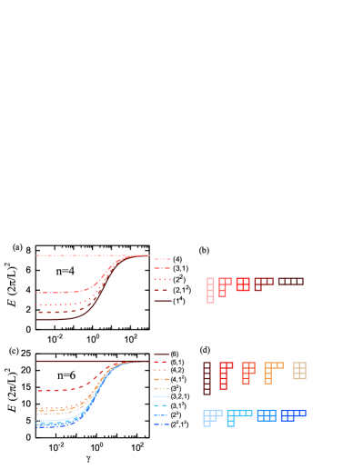
Figure 2: (color online). Ground state energies of states with different permutation symmetries versus the dimensionless interaction strength $\gamma$ for the $SU(4)$ system with particle number (a) $N=4$ and (c) $N=6$. (a) From dash-dot-dot line to solid line corresponding to the lowest-energy states with different symmetry classes described by the Young tableaux of the coordinate wave function in (b). (c) From the solid line to the dash-dot line corresponding to different symmetry classes described by the Young tableaux shown in (d).

Due to the unique correspondence between the symmetry classes and quantum numbers in the BAEs, we can calculate the lowest eigenenergy for each given symmetry class by numerically solving the corresponding BAEs with the quantum numbers $\left\{I_{j}\right\}=\left\{1,2,\cdots,N\right\}$ and $\{J_{\alpha}^{r}\}=\left\{1,2,\cdots,M_{r}\right\}$, which permits us to determine the order of energy levels with different symmetries. We present our results for the spin-$3/2$ fermionic gas with $SU\left(4\right)$ symmetry in Fig.2. For the case of $N=4$ with five sets of $\{M_{r}\}$, the corresponding lowest energies for each symmetry classes are shown in Fig.2(a), indicating that the order of the energy levels fulfills $E\left(4\right)>E\left(3,1\right)>E\left(2,2\right)>E\left(2,1^{2}\right)>E\left(1^{4}\right)$ in the whole regime $0\leq\gamma<\infty$, except in the Tonks-Girardeau limit $\gamma\rightarrow\infty$ all the levels approach the same value, where $\gamma=cL/N$ is the dimensionless interaction strength. We note that in this case, the order of energy levels can also be determined by applying the LMT II, as all the five different symmetry classes are comparable according to the pouring principle. However, for the case of $N=6$, there exist incomparable symmetry classes, as discussed before, neither $\left(4,1^{2}\right)$ nor $\left(3^{2}\right)$ can be poured into each other, so the LMT cannot determine the order of $E\left(4,1^{2}\right)$ and $E\left(3^{2}\right)$. Also, $E\left(3,1^{3}\right)$ and $E\left(2^{3}\right)$ are not comparable by the pouring principle. Similar to the case of $N=4$, all the symmetry classes for $N=6$ can be uniquely determined by solving the BAEs and thus we can give an order of the energy levels as demonstrated in Fig.2(c). From our calculated results, we can determine the order of energy levels of the incomparable symmetry classes and we have $E\left(4,1^{2}\right)>E\left(3^{2}\right)$ and $E\left(3,1^{3}\right)>E\left(2^{3}\right)$. As shown in Fig.2 (c), the order of ground state energies with different symmetries does not change for arbitrary finite interaction strength and no phase transition occurs in the whole repulsive interaction region.

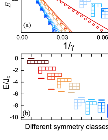
Figure 3: (color online). (a) The lowest energy versus $1/\gamma$ for various symmetry classes. The scattered symbols represent results obtained from the effective spin chain, whereas the solid lines are obtained by solving the BAES. (b) The lowest energy calculated by exact diagonalization of effective spin chain model of the $SU(4)$ system with $N=6$ in a harmonic trap for various symmetry classes. Here we use the Young tableaus of spin wave function, which conjugate with the tableaus of coordinate wave function in Fig.2(d), to represent different symmetry classes.

In the strongly repulsive regime $\left(cL/N\gg 1\right)$, spin rapidities $\lambda_{\alpha}^{\left(r\right)}$ are proportional to $c$ while $k_{j}$ remains finite. From the expansion of Eq.(2) up to the first order in $k_{j}/c$, the quasi-momentum is given by $2k_{j}L=2\pi I_{j}-2\zeta\frac{k_{j}}{c}+O\left(\left|c\right|^{-3}\right)$, which leads to $k_{j}=\frac{\pi}{L}I_{j}\left(1+\frac{1}{cL}\zeta\right)$ with

$$\zeta=\sum_{\alpha=1}^{M_{1}}\frac{4}{1+4(\gamma_{\alpha}^{1})^{2}}.$$ (4)

Here $\gamma_{\alpha}^{r}\equiv\lambda_{\alpha}^{r}/c$ and $\gamma_{\alpha}^{1}$ is determined by the following equation

$$2N\theta\left(2\gamma_{\alpha}^{1}\right) = 2\pi J_{\alpha}^{1}-\sum_{\beta\neq\alpha}^{M_{1}}\left[\theta\left(\gamma_{\alpha}^{1}-\gamma_{\beta}^{1}\right)+\theta\left(\gamma_{\alpha}^{1}+\gamma_{\beta}^{1}\right)\right]$$ (5)

$$-\sum_{\gamma=1}^{M_{2}}\left[\theta\left(2\gamma_{\alpha}^{1}-2\gamma_{\gamma}^{2}\right)+\theta\left(2\gamma_{\alpha}^{1}+2\gamma_{\gamma}^{2}\right)\right],$$

which is obtained from the expansion of the second BAEs, i.e., Eq.(3) with $r=1$, up to the first order in $k_{j}/c$. The above equation can not solely determine $\gamma_{\alpha}^{1}$ as it includes $\gamma_{\alpha}^{2}$, which should be iteratively determined by the following equations

$$\sum_{\beta\neq\alpha}^{M_{r}}\left[\theta\left(\gamma_{\alpha}^{r}-\gamma_{\beta}^{r}\right)+\theta\left(\gamma_{\alpha}^{r}+\gamma_{\beta}^{r}\right)\right]=2\pi J_{\alpha}^{r}+$$

$$~{}\sum_{\gamma=1}^{M_{r+1}}\left[\theta\left(2\gamma_{\alpha}^{r}-2\gamma_{\gamma}^{r+1}\right)+\theta\left(2\gamma_{\alpha}^{r}+2\gamma_{\gamma}^{r+1}\right)\right]+$$

$$~{}\sum_{\delta=1}^{M_{r-1}}\left[\theta\left(2\gamma_{\alpha}^{r}-2\gamma_{\delta}^{r-1}\right)+\theta\left(2\gamma_{\alpha}^{r}+2\gamma_{\delta}^{r-1}\right)\right],$$ (6)

with $\alpha=1,\cdots,M_{r}$ ($r=2,\cdots n-1$). Up to the order of $c^{-1}$, the ground state energy of the $SU(n)$ Fermi gas is given by

$$E=E_{F}\left(1-\frac{2}{cL}\zeta\right)=E_{F}\left(1-2\frac{\zeta/N}{\gamma}\right),$$ (7)

where $E_{F}=\frac{\hbar^{2}\pi^{2}}{2mL^{2}}\frac{2N^{3}+3N^{2}+N}{6}$ is the energy at $c=\infty$. It is equal to the Fermi energy of fully polarized Fermi gas, consistent with that from the generalized Bose-Fermi mapping Guan2006 ; Yang2009 ; Chen2009 ; Deuretzbacher ; Girardeau1 ; Girardeau2007 .

We note that Eq.(5) and (6) are the well-known Bethe equations for the open $SU(n)$ Heisenberg spin chain

$$H_{S}=J\sum_{i=1}^{N-1}(P_{i,i+1}-1),$$ (8)

here $P_{i,i+1}$ is the permutation operator which permutes the spin states of the $i$-th and $i+1$-th particles. The ground state energy of $H_{S}$ with $J>0$ is given by $E_{S}=-J\zeta$ Sutherland1975 . By comparing with Eq.(7), we see that the effective Hamiltonian describing the spin dynamics in the strongly interacting limit is given by $H_{eff}=H-E_{F}=H_{S}$ with the exchange parameter given by $J=2\frac{\epsilon_{F}}{\gamma}$, where $\epsilon_{F}=E_{F}/N$ is the average Fermi energy. In Fig.3(a), we show the energy spectrum of $H$ in the strongly repulsive limit for the uniform system with $N=6$ by using the effective Hamiltonian $H=E_{F}+H_{S}$. In the infinitely repulsive limit $\gamma\rightarrow\infty$, all the energy levels of different symmetry classes are degenerate. Since the ground state energies of $H_{S}$ for systems belonging to different symmetry classes take different values, the energy levels split when the interaction strength deviates the TG limit. The order of the splitting levels are convenient to be distinguished by the Young diagrams of the spin wavefuntion, which are the conjugations of the Young diagrams of the coordinate wavefuntion (see Fig.1).

In the strongly interacting regime, the $SU(n)$ Fermi gas in an inhomogeneous potential can also be described by a non-uniform effective spin-chain model

$$H_{eff}=\sum_{i=1}^{N-1}J_{i}(P_{i,i+1}-1),$$ (9)

with the coefficients given by

$$J_{i}=\frac{2N!}{c}\int\prod_{j}dx_{j}|\partial_{i}\varphi_{A}|^{2}\delta(x_{i}-x_{i+1})\theta_{[i,i+1]}^{1},$$

where $\theta_{[i,i+1]}^{1}=\theta^{1}/\theta(x_{i}-x_{i+1})$ is a reduced sector function, $\theta^{1}$ being the Heaviside step function whose value is $1$ in the region $x_{1}<x_{2}<\cdots<x_{N}$ and zero otherwise YangLi1 ; Lijun . The wave function $\varphi_{A}$ is taken as the ground state of $N$ spinless fermions, i.e., the Slater determinant made up of the lowest $N$-level of eigenstates. The difference from the uniform system is that the exchange coefficients are site-dependent. A generalization of LMT for the $SU(n)$ chain is given in Ref.Hakobyan . Consider the $SU(4)$ system with $N=6$ in a harmonic trap $V(x)=m\omega^{2}x^{2}/2$ with the trapping frequency $\omega$, we get a nonuniform $SU(4)$ spin chain with $J_{3}\equiv J_{c}$, $J_{1}=J_{5}=0.5743J_{c}$ and $J_{2}=J_{4}=0.8956J_{c}$, where $J_{c}$ represents the effective exchange strength between two spins in the trap center. By directly diagonalizing the corresponding spin chain model, we can get the order of energy levels for the harmonic system in the strong interaction strength region. As shown in Fig. 3(b), the order of energy levels is solely related to their symmetry classes, which agrees with the case of uniform system. Our result indicates that the order of energy levels in the strongly interacting regime is not changed when the trap potential is changed from the hard wall to the harmonic trap. Strongly interacting systems trapped in other external traps can be also studied similarly by solving corresponding effective spin-exchange models.

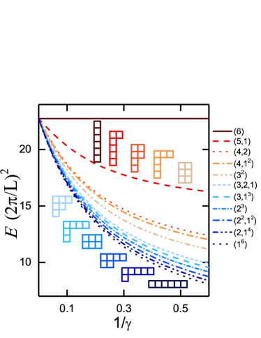
Figure 4: (color online). The ground state energies of eleven symmetry classes versus $1/\gamma$ for the $SU(6)$ system with $N=6$. From dark red solid line to dark blue dotted line correspond to the lowest energy states of different symmetry classes described by the corresponding Young tableaus.

Our results can be directly generalized to the multi-component $SU(n)$ system with larger $n$, for example, the system with $SU\left(6\right)$ symmetry, for which the BAEs take the form of Eqs. (2) and (3) with $n=6$. For the example system with $N=6$, by solving the corresponding BAEs, we can get the ground state energies for eleven symmetry classes. The corresponding results are shown in Fig.4. Compared to the case of $SU\left(4\right)$, there are two extra symmetry classes $(2,1^{4})$ and $(1^{6})$, and similarly there also exist incomparable symmetry classes by the pouring principle, e.g., $(4,1^{2})$ and $(3^{2})$, as well as $(3,1^{3})$ and $(2^{3})$. The exact BA result gives the order of ground state energy levels of different symmetry classes: $E(6)\geq E(5,1)\geq E(4,2)\geq\cdots\geq E(2,1^{4})\geq E(1^{6})$, where “$=$” holds true only in the TG limit $\gamma\rightarrow\infty$. As shown in Fig.4, the order is unchanged in the whole interaction region.

III SUMMARY

In summary, based on the BA solution of few-particle systems, we have studied the ordering of energy levels for all kinds of permutation symmetry classes of 1D multi-component Fermi systems with $SU(n)$ symmetry. In the strongly interacting regime, from the expansion of the BA solutions, we demonstrate that the system can be effectively described by an $SU(n)$ spin exchange model with the exchange parameter being exactly determined. Furthermore, the ordering of energy levels of the strongly interacting system trapped in a harmonic potential is also determined by solving its effective spin-exchange model.

- (1) I. Bloch, J. Dalibard, and W. Zwerger, Rev. Mod. Phys. 80, 885 (2008).
- (2) T. B. Ottenstein, T. Lompe, M. Kohnen, A. N. Wenz, and S. Jochim, Phys. Rev. Lett. 101, 203202 (2008).
- (3) J. H. Huckans, J. R. Williams, E. L. Hazlett, R. W. Stites, and K. M. O’Hara, Phys. Rev. Lett. 102, 165302 (2009).
- (4) X. Zhang, M. Bishof, S. L. Bromley, C. V. Kraus, M. S. Safronova, P. Zoller, A. M. Rey, and J. Ye, Science 345 1467 (2014).
- (5) F. Scazza, C. Hofrichter, M. Höfer, P. C. De Groot, I. Bloch, and S. Fölling, Nat. Phys. 10, 779(2014).
- (6) G. Cappellini, M. Mancini, G. Pagano, P. Lombardi, L. Livi, M. Siciliani de Cumis, P. Cancio, M. Pizzocaro, D. Calonico, F. Levi, C. Sias, J. Catani, M. Inguscio, and L. Fallani, Phys. Rev. Lett. 113, 120402 (2014).
- (7) M. A. Cazalilla, A. F. Ho, and M. Ueda, New J. Phys. 11, 103033 (2009).
- (8) S. Taie, Y. Takasu, S. Sugawa, R. Yamazaki, T. Tsujimoto, R. Murakami, and Y. Takahashi, Phys. Rev. Lett. 105, 190401 (2010).
- (9) C. Hofrichter, L. Riegger, F. Scazza, M. Höfer, D. R. Fernandes, I. Bloch, and S. Fölling, Phys. Rev. X 6, 021030 (2016).
- (10) G. Pagano, M. Mancini, G. Cappellini, P. Lombardi, F. Schäfer, H. Hu, X.-J. Liu, J. Catani, C. Sias, M. Inguscio, and L. Fallani, Nat. Phys. 10, 198 (2014).
- (11) C. Wu, Phys. Rev. Lett. 95, 266404 (2005); C. Wu, J. P. Hu, and S. C. Zhang, Phys. Rev. Lett. 91, 186402 (2003).
- (12) S. Chen, C. Wu, S. C. Zhang, and Y. Wang, Phys. Rev. B 72, 214428 (2005).
- (13) D. Wang, Y. Li, Z. Cai, Z. Zhou, Y. Wang, and C. Wu, Phys. Rev. Lett. 112, 156403 (2014).
- (14) P. Nataf and F. Mila, Phys. Rev. Lett. 113, 127204 (2014).
- (15) A. G. Volosniev, D. V. Fedorov, A. S. Jensen, M. Valiente, and N. T. Zinner, Nat. Commun. 5, 5300 (2014).
- (16) F. Deuretzbacher, D. Becker, J. Bjerlin, S. M. Reimann, and L. Santos, Phys. Rev. A 90, 013611 (2014).
- (17) A. G. Volosniev, D. Petrosyan, M. Valiente, D. V. Fedorov, A. S. Jensen, and N. T. Zinner, Phys. Rev. A 91, 023620 (2015).
- (18) J. Levinsen, P. Massignan, G. M. Bruun, and, M. M. Parish, Sci. Adv. 1, e1500197 (2015).
- (19) P. Massignan, J. Levinsen, and M. M. Parish, Phys. Rev. Lett. 115, 247202 (2015).
- (20) F. Deuretzbacher, D. Becker, and L. Santos, Phys. Rev. A 94, 023606 (2016).
- (21) F. Deuretzbacher, D. Becker, J. Bjerlin, S. M. Reimann, L. Santos, Phys. Rev. A 95, 043630 (2017).
- (22) L. Yang, L. Guan, and H. Pu, Phys. Rev. A 91, 043634 (2015).
- (23) A. S. Dehkharghani, A. G. Volosniev, E. J. Lindgren, J. Rotureau, C. Forssn, D. V. Fedorov, A. S. Jensen, and N. T. Zinner, Scientific reports 5, 16075 (2015).
- (24) L. Yang and X. Cui, Phys. Rev. A 93, 013617 (2016).
- (25) H. Hu, L. Pan, and S. Chen, Phys. Rev. A 93, 033636 (2016)
- (26) L. Yang and H. Pu, Phys. Rev. A 94, 033614 (2016).
- (27) H. Hu, L. Guan, and S. Chen, New J. Phys. 18, 025009 (2016)
- (28) F. Deuretzbacher, D. Becker, J. Bjerlin, S. M. Reimann, and L. Santos Phys. Rev. A 90, 013611 (2014).
- (29) A. G. Volosniev, Few-Body Syst 58: 54 (2017).
- (30) N. L. Harshman, Few-Body Syst 57: 45 (2016); Few-Body Syst 57: 11 (2016).
- (31) Z. Zhou, Z. Cai, C. Wu, and Y. Wang, Phys. Rev. B 90, 235139 (2014).
- (32) V. Bois, S. Capponi, P. Lecheminant, M. Moliner, and K. Totsuka, Phys. Rev. B 91, 075121 (2015).
- (33) J. Decamp, J. Jüemann, M. Albert, M. Rizzi, A. Minguzzi, and P. Vignolo, Phys. Rev. A 90, 053614 (2016).
- (34) M. E. Beverland, G. Alagic, M. J. Martin, A. P. Koller, A. M. Rey, and A. V. Gorshko, Phys. Rev. A 93, 051601(R) (2016).
- (35) P. Nataf, M. Lajkó, P. Corboz, A. M. Läuchli, K. Penc, and Frédéric Mila, Phys. Rev. B 93, 201113(R) (2016).
- (36) P. Nataf and F. Mila, Phys. Rev. B 93, 155134 (2016).
- (37) X.-W. Guan, Z.-Q. Ma, and B. Wilson, Phys. Rev. A 85, 033633 (2012); Y. Jiang, P. He, and X.-W. Guan, J. Phys. A: Math. Theor. 49, 174005 (2016).
- (38) S. Capponi, P. Lecheminant, and K. Totsuka, Ann. Phys. 367, 50 (2016).
- (39) E. Lieb and D. Mattis, Phys. Rev. 125, 164 (1962).
- (40) J. Decamp, P. Armagnat, B. Fang, M. Albert, A. Minguzzi, and P. Vignolo, New J. Phys. 18, 055011(2016).
- (41) B. Sutherland, Phys. Rev. Lett. 20, 98 (1968).
- (42) M. Gaudin, Phys. Rev A, 4, 386 (1971).
- (43) N. Oelkers, M. T. Batchelor, M. Bortz, and X.-W. Guan, J. Phys. A: Math. Gen. 39, 1073 (2006).
- (44) C. N. Yang, Chin. Phys. Let. 26, 120504 (2009).
- (45) M. D. Girardeau and A. Minguizzi, Phys. Rev. Lett. 99, 230402 (2007).
- (46) F. Deuretzbacher, K. Fredenhagen, D. Becker, K. Bongs, K. Sengstock, and D. Pfannkuche, Phys. Rev. Lett. 100, 160405 (2008).
- (47) L. Guan, S. Chen, Y. Wang and Z. Q. Ma, Phys. Rev. Lett. 102, 160402 (2009).
- (48) M. D. Girardeau, J. Math. Phys. 1, 516 (1960).
- (49) B. Sutherland, Phys. Rev. B 12, 3795 (1975).
- (50) T. Hakobyan, Nucl. Phys. B 699, 575, (2004); T. Hakobyan, SIGMA 6, 024, (2010).