Pattern Storage, Bifurcations and Higher-Order Correlation Structure of an Exactly Solvable Asymmetric Neural Network Model

Diego Fasoli^1,2,∗, Anna Cattani¹, Stefano Panzeri¹

1 Laboratory of Neural Computation, Center for Neuroscience and Cognitive Systems @UniTn, Istituto Italiano di Tecnologia, 38068 Rovereto, Italy

2 Center for Brain and Cognition, Computational Neuroscience Group, Universitat Pompeu Fabra, 08002 Barcelona, Spain

$\ast$ Corresponding Author. E-mail: diego.fasoli@upf.edu

Abstract

Exactly solvable neural network models with asymmetric weights are rare, and exact solutions are available only in some mean-field approaches. In this article we find exact analytical solutions of an asymmetric spin-glass-like model of arbitrary size and we perform a complete study of its dynamical and statistical properties. The network has discrete-time evolution equations, binary firing rates and can be driven by noise with any distribution. We find analytical expressions of the conditional and stationary joint probability distributions of the membrane potentials and the firing rates. The conditional probability distribution of the firing rates allows us to introduce a new learning rule to store safely, under the presence of noise, point and cyclic attractors, with important applications in the field of content-addressable memories. Furthermore, we study the neuronal dynamics in terms of the bifurcation structure of the network. We derive analytically examples of the codimension one and codimension two bifurcation diagrams of the network, which describe how the neuronal dynamics changes with the external stimuli. In particular, we find that the network may undergo transitions among multistable regimes, oscillatory behavior elicited by asymmetric synaptic connections, and various forms of spontaneous symmetry-breaking. On the other hand, the joint probability distributions allow us to calculate analytically the higher-order correlation structure of the network, which reveals neuronal regimes where, statistically, the membrane potentials and the firing rates are either synchronous or asynchronous. Our results are valid for networks composed of an arbitrary number of neurons, but for completeness we also derive the network equations in the mean-field limit and we study analytically their local bifurcations. All the analytical results are extensively validated by numerical simulations.

1 Introduction

In biological neural networks, asymmetric synapses constitute $75-95\%$ of all synapses [8]. Yet, exactly solvable neural network models with asymmetric synaptic connections are rare. Typically, asymmetric models that admit exact solutions are spin-glass-like systems of neural networks, such as the Little-Hopfield model [23, 21] and the Sherrington-Kirkpatrick model [34, 26]. In neuroscience, these models were investigated in the ’$70$s and ’$80$s, during a renewed interest in neural networks that followed the pioneer work on the McCulloch-Pitts model [24] and the Perceptron [33] (’$40$s and ’$50$s respectively). Due to their complexity, spin-glass-like models admit exact analytical solutions only in some mean-field approaches. In [20], Hertz et al. solved the Langevin dynamics of the $n$-component soft-spin version of the asymmetric Sherrington-Kirkpatrick model in the limit $n\rightarrow\infty$. In [6], Crisanti and Sompolinsky found exact analytical expressions for the average autocorrelation and susceptibility of a spherical asymmetric spin-glass model in the mean-field limit of infinite network size. In [31], Rieger et al. found exact solutions for the response and autocorrelation functions of a fully asymmetric Sherrington-Kirkpatrick model, by means of a path-integral approach. Moreover, in [9] Derrida et al. found an analytical expression of the evolution of a spin configuration having a finite overlap on one stored pattern in a dilute version of the asymmetric Little-Hopfield model. Since spin-glasses display features that are widespread in complex systems, nowadays the interest in these models is still strong in fields of research such as mathematics, physics, chemistry, and materials science [4].

The main difficulty in studying asymmetric neural networks is the impossibility to apply the powerful methods of equilibrium statistical mechanics, because no energy function exists for these systems. In this work, we introduce an asymmetric spin-glass like neural network model with random noise (Sec. (2)) that can be solved exactly without adopting any mean-field approach (Sec. (3)). In particular, our solutions are valid for networks composed of an arbitrary number of neurons, and do not require additional constraints such as synaptic dilution.

Despite most of the work on spin-glass-like neural networks dates back to the ’$70$s and ’$80$s, we set our study in the modern context of bifurcation theory and functional connectivity analysis, which nowadays are topics of central importance to systems neuroscience [12, 13]. In SubSec. (3.1) we derive exact analytical solutions for the conditional probability distributions of the membrane potentials and the firing rates, as well as for the joint probability distributions in the stationary regime. In SubSec. (3.2) we show that the conditional probability distribution of the firing rates allows us to define a new learning rule to safely store stationary and oscillating solutions even in presence of noise. In SubSec. (3.3) we derive examples of exact codimension one and codimension two bifurcation diagrams in the zero-noise limit of the network equations. Then, in SubSec. (3.4) we calculate the higher-order correlation structure of the noisy network, for both the membrane potentials and the firing rates. While all the results are valid for networks composed of an arbitrary number of neurons, for completeness in SubSec. (3.5) we also derive the mean-field equations in the thermodynamic limit $N\rightarrow\infty$, and we find exact analytical expressions of the local codimension one bifurcations. To conclude, in Sec. (4) we discuss the novelty and the biological implications of our results.

2 Materials and Methods

In this section we introduce the neural network model we study. For the sake of clarity, in the main text of this article we suppose that the network is driven by independent noise sources with Gaussian distribution, while in the Supplementary Materials we consider noise with arbitrary distribution.

Here we describe the neuronal activity by means of the following spin-glass-like network model:

$$V_{i}\left(t+1\right)=\frac{1}{M_{i}}\sum_{j=0}^{N-1}J_{ij}\mathscr{H}\left(V_{j}\left(t\right)-\theta_{j}\right)+I_{i}\left(t\right)+\sigma_{i}^{\mathcal{B}}\mathcal{B}_{i}\left(t\right),\quad i=0,...,N-1.$$ (1)

The network is synchronously updated, which is considered a more realistic description of the biological dynamics [11, 27]. Moreover, in Eq. (1) $N\geq 2$ represents the number of neurons in the network and is generally finite. $V_{i}\left(t+1\right)$ is the membrane potential of the $i$th neuron at the time instant $t+1$. The external current $I_{i}\left(t\right)$ is the deterministic component of the stimulus to the $i$th neuron. $\sigma_{i}^{\mathcal{B}}\mathcal{B}_{i}$ is the stochastic component of the stimulus, where $\mathcal{B}_{i}\left(t\right)$ for $i=0,...,N-1$ are independent normally distributed noise sources with unit variance. $\sigma_{i}^{\mathcal{B}}$ represents the overall intensity (i.e. the standard deviation) of the noisy term. Moreover, $\mathscr{H}\left(\cdot\right)$ is the Heaviside step function with threshold $\theta$:

$$\mathscr{H}\left(V-\theta\right)=\begin{cases}0&\mathrm{if}\;V\leq\theta\\ \\ 1&\mathrm{otherwise},\end{cases}$$ (2)

which converts the membrane potential of the $j$th neuron into its corresponding binary firing rate, $\nu_{j}\left(t\right)=\mathscr{H}\left(V_{j}\left(t\right)-\theta_{j}\right)\in\left\{0,1\right\}$. Then, $J_{ij}$ is the synaptic weight from the $j$th (presynaptic) neuron to the $i$th (postsynaptic) neuron. In this article, the matrix $J$ is arbitrary, therefore it may be asymmetric and self-connections (loops) may be present. $M_{i}$ is the total number of incoming connections to the $i$th neuron, and represents a normalization factor that prevents the divergence of the sum $\sum_{j=0}^{N-1}J_{ij}\mathscr{A}\left(V_{j}\left(t\right)\right)$ for large networks.

In the special case when $J$ is symmetric, invertible and with zeros on the main diagonal ($J_{ii}=0$), while $I_{i}=\sigma_{i}^{\mathcal{B}}=0\;\forall i$, under the following change of variables:

$$V_{i}\left(t\right)=\frac{1}{M_{i}}\sum_{j=0}^{N-1}J_{ij}A_{j}\left(t\right),$$

Eq. (1) is equivalent to the synchronous version of the network model introduced by Hopfield in [21]:

$$A_{i}\left(t+1\right)=\mathscr{H}\left(\frac{1}{M_{i}}\sum_{j=0}^{N-1}J_{ij}A_{j}\left(t\right)-\theta_{i}\right),\quad i=0,...,N-1.$$

Important differences arise in the asymmetric model, as we discuss in the next section.

3 Results

In this section we study the dynamical and statistical properties of the network equations (1). In SubSec. (3.1) we report the exact solutions of the conditional probability distributions of the membrane potentials and the firing rates, as well as the joint probability distributions in the stationary regime. Then, in SubSec. (3.2) we invert the formula of the conditional probability distribution of the firing rates, which allows us to define a new learning rule to safely store stationary and oscillatory patterns of neural activity even in presence of noise. In SubSec. (3.3) we study analytically the bifurcations of the network dynamics in the zero-noise limit $\sigma^{\mathcal{B}}\rightarrow 0$, in terms of its codimension one and codimension two bifurcation diagrams. In SubSec. (3.4) we derive exact analytical expressions for the higher-order cross-correlations of the membrane potentials and the firing rates, for any noise intensity. To conclude, in SubSec. (3.5) we report the mean-field equations of the network, which are exact in the thermodynamic limit $N\rightarrow\infty$, and we study analytically its local bifurcations. All the analytical results are extensively validated by numerical simulations.

3.1 Conditional and Joint Probability Distributions

We call $\boldsymbol{V}=\left[\begin{array}[t]{ccc}V_{0},&\ldots,&V_{N-1}\end{array}\right]^{T}$ the collection of the membrane potentials at time $t+1$, and $\boldsymbol{V}^{\prime}$ that at time $t$. In the Supplementary Materials (see SubSec. (S1.1.3)) we prove that if the membrane potentials evolve in time according to Eq. (1), then their conditional probability distribution is:

$$p\left(\boldsymbol{V}|\boldsymbol{V}^{\prime}\right)=\frac{1}{\left(2\pi\right)^{\frac{N}{2}}\prod_{i=0}^{N-1}\sigma_{i}^{\mathcal{B}}}\prod_{m=0}^{N-1}e^{-\frac{1}{2}\left(\frac{V_{m}-\frac{1}{M_{m}}\sum_{n=0}^{N-1}J_{mn}\mathscr{H}\left(V^{\prime}_{n}-\theta_{n}\right)-I_{m}\left(t\right)}{\sigma_{m}^{\mathcal{B}}}\right)^{2}}.$$ (3)

Eq. (3) holds for any $t$ and also for time-varying stimuli $I_{i}\left(t\right)$. Moreover, if the network statistics reach a stationary regime (typically this occurs for $t\rightarrow\infty$ and for constant stimuli $I_{i}\left(t\right)=I_{i}\;\forall t$), the joint probability distribution of the membrane potentials is:

$$p\left(\boldsymbol{V}\right)=\frac{1}{\left(2\pi\right)^{\frac{N}{2}}\prod_{i=0}^{N-1}\sigma_{i}^{\mathcal{B}}}\sum_{j=0}^{2^{N}-1}F_{j}\prod_{m=0}^{N-1}e^{-\frac{1}{2}\left(\frac{V_{m}-\frac{1}{M_{m}}\sum_{n=0}^{N-1}J_{mn}\mathscr{B}_{j,n}^{\left(N\right)}-I_{m}}{\sigma_{m}^{\mathcal{B}}}\right)^{2}}.$$ (4)

In Eq. 4, $\mathscr{B}_{j,n}^{\left(N\right)}\overset{\mathrm{def}}{=}\left[\boldsymbol{\mathscr{B}}_{j}^{\left(N\right)}\right]_{n}$, and $\boldsymbol{\mathscr{B}}_{j}^{\left(N\right)}$ is the $N\times 1$ vector whose entries are the digits of the binary representation of $j$ (e.g. $\boldsymbol{\mathscr{B}}_{5}^{\left(4\right)}=\left[\begin{array}[]{cccc}0,&1,&0,&1\end{array}\right]^{T}$, so that $\mathscr{B}_{5,0}^{\left(4\right)}=\mathscr{B}_{5,2}^{\left(4\right)}=0$ and $\mathscr{B}_{5,1}^{\left(4\right)}=\mathscr{B}_{5,3}^{\left(4\right)}=1$). If we define $\widetilde{\boldsymbol{F}}\overset{\mathrm{def}}{=}\left[\begin{array}[]{ccc}F_{0},&\ldots,&F_{2^{N}-2}\end{array}\right]^{T}$, then:

$$\widetilde{\boldsymbol{F}}=\mathcal{A}^{-1}\widetilde{\boldsymbol{G}},$$

while $F_{2^{N}-1}=1-\sum_{j=0}^{2^{N}-2}F_{j}$. Moreover, $\mathcal{A}$ and $\widetilde{\boldsymbol{G}}$ are a $\left(2^{N}-1\right)\times\left(2^{N}-1\right)$ matrix and a $\left(2^{N}-1\right)\times 1$ column vector respectively, defined as follows:

$$\mathcal{A}_{i,j}=\delta_{i,j}+G_{i,2^{N}-1}-G_{i,j}$$

$$\left[\widetilde{\boldsymbol{G}}\right]_{i}=G_{i,2^{N}-1}$$

$$G_{i,j}=\frac{1}{2^{N}}\prod_{m=0}^{N-1}\left[1+\left(-1\right)^{\mathscr{B}_{i,m}^{\left(N\right)}}\mathrm{erf}\left(\frac{\theta_{m}-\frac{1}{M_{m}}\sum_{n=0}^{N-1}J_{mn}\mathscr{B}_{j,n}^{\left(N\right)}-I_{m}}{\sqrt{2}\sigma_{m}^{\mathcal{B}}}\right)\right],$$

while $\delta_{i,j}$ is the Kronecker delta. $\mathcal{A}^{-1}$ can be calculated analytically from the cofactor matrix $\mathcal{C}$ of $\mathcal{A}$, through the relation $\mathcal{A}^{-1}=\frac{1}{\det\left(\mathcal{A}\right)}\mathcal{C}^{T}$, with $\det\left(\mathcal{A}\right)=\sum_{j=0}^{N-1}\mathcal{C}_{ij}\mathcal{A}_{ij}$ (for any $i$) according to Laplace’s formula. Then, from Eq. (4) we obtain the following expression of the single-neuron marginal probability distribution:

$$p_{i}\left(V\right)=\frac{1}{\sqrt{2\pi}\sigma_{i}^{\mathcal{B}}}\sum_{j=0}^{2^{N}-1}F_{j}e^{-\frac{1}{2}\left(\frac{V-\frac{1}{M_{i}}\sum_{k=0}^{N-1}J_{ik}\mathscr{B}_{j,k}^{\left(N\right)}-I_{i}}{\sigma_{i}^{\mathcal{B}}}\right)^{2}},\quad i=0,\ldots N-1.$$ (5)

Examples of the probability distributions of the membrane potentials for $N=2$ and $N=5$ are shown in Fig. (1) and in the top panels of Fig. (3), respectively.

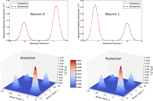
Figure 1: Examples of probability distributions for $\boldsymbol{N=2}$. This figure is obtained for the values of the parameters in Tab. (1). The red curves in the top panels show the single-neuron marginal probability distributions of the two neurons, as given by Eq. (5). The blue dots represent the numerical evaluation of the same distributions. The bottom panels show the two-neurons joint probability distribution, as given by Eq. (4) (left), and numerically evaluated (right). The numerical distributions of this figure have been obtained through a Monte Carlo method over $10^{6}$ repetitions of the network dynamics, obtained by solving iteratively Eq. (1) in the temporal interval $t=\left[0,100\right]$. Then, the probability distributions have been evaluated from the collected data at $t=100$ through a kernel density estimator. We assume that at $t=100$ the probability distributions have already reached a stationary regime, which is confirmed by the good agreement between the analytical and numerical results.

Figure 2: An example of oscillatory dynamics for $\boldsymbol{N=2}$. This figure is obtained for the values of the parameters in Tab. (1), and shows an example of oscillatory dynamics that corresponds to the stationary probability distributions of Fig. (1). The synchronous version of the Hopfield network (which has symmetric connections) can sustain only oscillations with period $\mathcal{T}=2$, known as two-cycles [17]. Here we show that the asymmetric network can undergo oscillations with period $\mathcal{T}=4$. The oscillations are perturbed by the presence of the noisy terms $\sigma_{i}^{\mathcal{B}}\mathcal{B}_{i}\left(t\right)$, while oscillations with $\mathcal{T}>2$ in the noise-free version of the model are shown in Fig. (7). The top-left panel shows an example of temporal dynamics of the membrane potentials during the oscillation, while the top-right panel shows the dynamics in the phase space of the model. The bottom-left panel shows the transition probabilities between the four possible states of the firing rates $\boldsymbol{\nu}$, according to Eq. (6). Then, the bottom-right panel shows the comparison between the analytical joint probability distribution of the firing rates (red bars, calculated by Eq. (7)), and the corresponding numerical distribution (blue bars).

Figure 3: Examples of probability distributions for $\boldsymbol{N=5}$. This figure is obtained for the values of the parameters in Tab. (2). The top panels show two examples of the single-neuron marginal probability distributions of the membrane potentials. The bottom-left panel shows the Kullback–Leibler divergence between the analytical single-neuron distributions (as given by Eq. (5)), and the corresponding numerical distributions (calculated as in Fig. (1)), for an increasing number of Monte Carlo repetitions (trials) of the network dynamics. The divergence decreases with the number of repetitions, therefore the numerical distribution is better approximated by its analytical counterpart when the statistical error (due to the finite number of repetitions) decreases. The bottom-right panel shows the comparison between the analytical joint probability distribution of the firing rates (red bars, calculated by Eq. (7)), and the corresponding numerical distribution (blue bars), over the $2^{N}=16$ states of the network activity.

$J=\left[\begin{array}[]{cc}0&-11\\ 11&0\end{array}\right],\quad\boldsymbol{I}=\left[\begin{array}[]{c}1\\ -1\end{array}\right],\quad\boldsymbol{\sigma}^{\mathcal{B}}=\left[\begin{array}[]{c}1\\ 1\end{array}\right]$

Table 1: Set of parameters used for generating Figs. (1) and (2).

$J=\left[\begin{array}[]{ccccc}0&40&-36&60&-36\\ 104&0&-40&32&-40\\ 40&80&0&40&-8\\ 52&60&-56&0&-84\\ 36&64&-44&48&0\end{array}\right],\quad\boldsymbol{I}=\left[\begin{array}[]{c}-1\\ 0\\ -2\\ 2\\ 0\end{array}\right],\quad\boldsymbol{\sigma}^{\mathcal{B}}=\left[\begin{array}[]{c}2\\ 1\\ 1\\ 2\\ 3\end{array}\right]$

Table 2: Set of parameters used for generating Fig. (3).

Neuroscientists often make use of measures of correlation between firing rates, rather than between membrane potentials. For this reason, it is interesting to evaluate also the probability distributions of the firing rates, which in our model are binary quantities defined as $\nu_{i}\left(t\right)\overset{\mathrm{def}}{=}\mathscr{H}\left(V_{i}\left(t\right)-\theta_{i}\right)$. If we introduce the vector $\boldsymbol{\nu}=\left[\begin{array}[t]{ccc}\nu_{0},&\ldots,&\nu_{N-1}\end{array}\right]^{T}$, then from Eqs. (3) and (4) it is easy to prove (see SubSec. (S1.2.1) of the Supplementary Materials) that the conditional probability distribution, and the stationary joint and single-neuron marginal distributions of the firing rates are:

$$P\left(\boldsymbol{\nu}|\boldsymbol{\nu}^{\prime}\right)= \frac{1}{2^{N}}\prod_{m=0}^{N-1}\left[1+\left(-1\right)^{\nu_{m}}\mathrm{erf}\left(\frac{\theta_{m}-\frac{1}{M_{m}}\sum_{n=0}^{N-1}J_{mn}\nu_{n}^{\prime}-I_{m}\left(t\right)}{\sqrt{2}\sigma_{m}^{\mathcal{B}}}\right)\right]$$ (6)

$$P\left(\boldsymbol{\nu}\right)= \frac{1}{2^{N}}\sum_{j=0}^{2^{N}-1}F_{j}\prod_{m=0}^{N-1}\left[1+\left(-1\right)^{\nu_{m}}\mathrm{erf}\left(\frac{\theta_{m}-\frac{1}{M_{m}}\sum_{n=0}^{N-1}J_{mn}\mathscr{B}_{j,n}^{\left(N\right)}-I_{m}}{\sqrt{2}\sigma_{m}^{\mathcal{B}}}\right)\right]$$ (7)

$$P_{i}\left(\nu\right)= \frac{1}{2}\sum_{j=0}^{2^{N}-1}F_{j}\left[1+\left(-1\right)^{\nu}\mathrm{erf}\left(\frac{\theta_{i}-\frac{1}{M_{i}}\sum_{n=0}^{N-1}J_{in}\mathscr{B}_{j,n}^{\left(N\right)}-I_{i}}{\sqrt{2}\sigma_{i}^{\mathcal{B}}}\right)\right],\quad i=0,\ldots N-1$$ (8)

respectively. We observe that while Eqs. (3), (4) and (5) represent probability density functions (pdfs), namely probability distributions of continuous random variables (the membrane potentials), Eqs. (6), (7) and (8) represent probability mass functions (pmfs), namely probability distributions of discrete random variables (the firing rates). In particular, $P\left(\boldsymbol{\nu}|\boldsymbol{\nu}^{\prime}\right)$ is known as state-to-state transition probability matrix in the context of the theory of Markov processes [15]. Examples of $P\left(\boldsymbol{\nu}\right)$ for $N=2$ and $N=5$ are shown in the bottom-right panels of Figs. (2) and (3), respectively.

3.2 A New Learning Rule for Storing Point and Cyclic Attractors

At time $t$, the state of the neural network is described by the vector of the firing rates, $\boldsymbol{\nu}\left(t\right)=\left[\begin{array}[t]{ccc}\nu_{0}\left(t\right),&\ldots,&\nu_{N-1}\end{array}\left(t\right)\right]^{T}$, which represents the activity pattern of the system at time $t$. In the context of content-addressable memories, one aims to determine a synaptic connectivity matrix $J$ that stores one or more desired sequences of activity patterns. The way such matrix is built defines a learning rule for storing these patterns.

In particular, we suppose we want to store $D$ pattern sequences $\boldsymbol{\nu}^{\left(i\right)}\left(t_{0}\right)\rightarrow\ldots\rightarrow\boldsymbol{\nu}^{\left(i\right)}\left(t_{L_{i}}\right)$ of length $L_{i}$, for $i=0,\ldots,D-1$. By inverting Eq. (6), in Sec. (S2) of the Supplementary Materials we prove that if the network is fully-connected without loops, the matrix $J$ that stores these pattern sequences satisfies the following sets of linear algebraic equations:

$$\Omega^{\left(j\right)}\boldsymbol{J}^{\left(j\right)}=\boldsymbol{u}^{\left(j\right)},\quad j=0,\ldots,N-1.$$ (9)

In Eq. (9), $\boldsymbol{J}^{\left(j\right)}$ is the $\left(N-1\right)\times 1$ vector with entries $J_{jk}$ for $k\neq j$ (the weights $J_{jj}$ are equal to zero, therefore they are already known). Moreover, if we define $\mathcal{L}\overset{\mathrm{def}}{=}\sum_{i=0}^{D-1}L_{i}$ and $L_{-1}\overset{\mathrm{def}}{=}0$, then $\boldsymbol{u}^{\left(j\right)}$ is a $\mathcal{L}\times 1$ vector with entries:

$$u_{L_{i-1}+n_{i}}^{\left(j\right)}=\left(N-1\right)\left[\theta_{j}-\left(-1\right)^{\nu_{j}^{\left(i\right)}\left(t_{n_{i}}+1\right)}K_{j}^{\left(i,n_{i}\right)}\sqrt{2}\sigma_{j}^{\mathcal{B}}-I_{j}\right],\quad n_{i}=0,\ldots,L_{i}-1,\quad i=0,\ldots,D-1,$$

where $K_{j}^{\left(i,n_{i}\right)}$ is any sufficiently large and positive constant. Moreover, $\Omega^{\left(j\right)}$ is the $\mathcal{L}\times\left(N-1\right)$ matrix obtained by removing the $j$th column of the matrix:

$$\Omega=\left[\begin{array}[]{ccc}\nu_{0}^{\left(0\right)}\left(t_{0}\right)&\ldots&\nu_{N-1}^{\left(0\right)}\left(t_{0}\right)\\ \vdots&\ddots&\vdots\\ \nu_{0}^{\left(0\right)}\left(t_{L_{0}-1}\right)&\ldots&\nu_{N-1}^{\left(0\right)}\left(t_{L_{0}-1}\right)\\ \vdots&\ddots&\vdots\\ \nu_{0}^{\left(D-1\right)}\left(t_{0}\right)&\ldots&\nu_{N-1}^{\left(D-1\right)}\left(t_{0}\right)\\ \vdots&\ddots&\vdots\\ \nu_{0}^{\left(D-1\right)}\left(t_{L_{D-1}-1}\right)&\ldots&\nu_{N-1}^{\left(D-1\right)}\left(t_{L_{D-1}-1}\right)\end{array}\right].$$

Generally, each system in Eq. (9) may be solved through the pseudoinverse of the matrix $\Omega^{\left(j\right)}$, providing the set of synaptic weights that store the $D$ pattern sequences $\boldsymbol{\nu}^{\left(i\right)}\left(t_{0}\right)\rightarrow\ldots\rightarrow\boldsymbol{\nu}^{\left(i\right)}\left(t_{L_{i}}\right)$ (even though solutions to Eq. (9) do not always exist, depending on $\Omega^{\left(j\right)}$ and $\boldsymbol{u}^{\left(j\right)}$).

In particular, we observe that oscillations of period $\mathcal{T}$ correspond to the special case $L_{i}=\mathcal{T}$ with $\boldsymbol{\nu}^{\left(i\right)}\left(t\right)=\boldsymbol{\nu}^{\left(i\right)}\left(t+\mathcal{T}\right)$. For $\mathcal{T}=1$ this condition allows us to store a stationary state. Examples of $\mathcal{M}$-stable systems obtained through this method are shown in Fig. (4), for $\mathcal{M}=2,\,3,\,4$, while examples of oscillatory dynamics with period $\mathcal{T}=2,\,3,\,4$ are shown in Fig. (5).

The learning rule Eq. (9) can be easily extended by including further constraints. For example, it is possible to relax the full-connectivity assumption and to set a given portion of the synaptic weights to zero. This allows us to define a learning rule for sparse neural networks. The storage capacity depends on the number of synaptic connections, but a detailed investigation is beyond the purpose of this article.

Figure 4: Neuronal multistability. Examples of stationary states stored in a network of size $N=4$, by means of the learning rule (9). $\mathcal{M}$ represents the degree of multistability of the network, namely the total number of stationary states. This figure plots the transitions between the states of the network (from $0_{10}=0000_{2}$ to $15_{10}=1111_{2}$), and the color of the arrows is determined by $P\left(\boldsymbol{\nu}|\boldsymbol{\nu}^{\prime}\right)$ (see Eq. (6)) for the values of the parameters in Tab. (3). The stationary states are highlighted in red.

$J=\left[\begin{array}[]{cccc}0&-39&93&-39\\ -84&0&-84&171\\ 123&-66&0&-66\\ -15&54&-15&0\end{array}\right],\quad J=\left[\begin{array}[]{cccc}0&-123&48&48\\ -510&0&171&171\\ 378&123&0&-255\\ 138&54&-84&0\end{array}\right],\quad J=\left[\begin{array}[]{cccc}0&93&93&-171\\ 171&0&-339&171\\ 123&-255&0&123\\ -84&54&54&0\end{array}\right]$

$\boldsymbol{I}=\left[\begin{array}[]{c}-2\\ 1\\ 2\\ -3\end{array}\right],\quad\boldsymbol{\sigma}^{\mathcal{B}}=\left[\begin{array}[]{c}2\\ 4\\ 3\\ 1\end{array}\right]$

Table 3: Set of parameters used for generating Fig. (4). The synaptic connectivity matrices $J$ have been obtained from Eq. (9) for $K_{j}^{\left(i,n_{i}\right)}=10\;\forall i,\,j,\,n_{i}$.

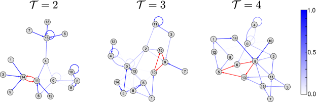
Figure 5: Neuronal oscillations. Examples of oscillatory states with period $\mathcal{T}$ stored in a network of size $N=4$, by means of the learning rule (9). This figure plots the conditional probability $P\left(\boldsymbol{\nu}|\boldsymbol{\nu}^{\prime}\right)$ for the values of the parameters in Tab. (4). The oscillatory states are highlighted in red..

$J=\left[\begin{array}[]{cccc}0&30&63&30\\ -84&0&-84&339\\ 84&42&0&42\\ -15&84&-15&0\end{array}\right],\quad J=\left[\begin{array}[]{cccc}0&-93&93&93\\ 171&0&3&-339\\ 123&-255&0&3\\ -30&3&84&0\end{array}\right],\quad J=\left[\begin{array}[]{cccc}0&-84&93&-84\\ -171&0&171&-171\\ 42&42&0&42\\ -42&-42&54&0\end{array}\right]$

Table 4: Set of parameters used for generating Fig. (5) ($\boldsymbol{I}$ and $\boldsymbol{\sigma}^{\mathcal{B}}$ as in Tab. (3)). The synaptic connectivity matrices $J$ have been obtained from Eq. (9) for $K_{j}^{\left(i,n_{i}\right)}=10\;\forall i,\,j,\,n_{i}$.

3.3 Bifurcations in the Deterministic Network

Bifurcation analysis is a mathematical technique for investigating the qualitative change in the neuronal dynamics produced by varying model parameters. Therefore it represents a fundamental tool for performing a systematic analysis of the complexity of the neuronal activity patterns. In particular, in this subsection we study how the dynamics of the network depends on the external stimuli $I_{i}$. Moreover, we perform our analysis in the zero-noise limit $\sigma^{\mathcal{B}}\rightarrow 0$, as is common practice in bifurcation theory (see e.g. [3, 18, 19, 12]). We observe that while local bifurcation analysis in graded models is performed through the eigenvalues of the Jacobian matrix [22], in our case an alternative approach is required. Indeed, the Jacobian matrix of our model is not defined at the discontinuity of the activation function (2), thus preventing the use of the powerful methods of bifurcation analysis developed for graded models.

Since we study the bifurcations in terms of formation/destruction of stationary and oscillatory solutions, the bifurcation diagrams of Eq. (1) can be obtained analytically from the conditional probability distribution of the firing rates $P\left(\boldsymbol{\nu}|\boldsymbol{\nu}^{\prime}\right)$ (see Eq. (6)), which in the zero-noise limit $\sigma^{\mathcal{B}}\rightarrow 0$ becomes:

$$P\left(\boldsymbol{\nu}|\boldsymbol{\nu}^{\prime}\right)=\frac{1}{2^{N}}\prod_{j=0}^{N-1}\left[1+\left(-1\right)^{\nu_{j}}\mathrm{sgn}\left(\theta_{j}-\frac{1}{M_{j}}\sum_{k=0}^{N-1}J_{jk}\nu_{k}^{\prime}-I_{j}\right)\right].$$ (10)

In Eq. (10), $\mathrm{sgn}\left(\cdot\right)$ is the sign function, which is defined as follows:

$$\mathrm{sgn}\left(x\right)=\begin{cases}-1&\mathrm{if}\;x<0\\ \\ \hphantom{-}1&\mathrm{otherwise}.\end{cases}$$

In particular, the stationary states $\boldsymbol{\nu}$ satisfy the condition $P\left(\boldsymbol{\nu}|\boldsymbol{\nu}\right)=1$. Therefore, if the stationary states were known, it would be possible to invert the condition $P\left(\boldsymbol{\nu}|\boldsymbol{\nu}\right)=1$ in the currents $I_{i}$, obtaining analytical expressions of the range of the stimuli where the network admits the stationary solution $\boldsymbol{\nu}$. In a similar way, each oscillatory solution of the network has to satisfy the condition $P\left(\boldsymbol{\nu}|\boldsymbol{\nu}^{\prime}\right)=1$ at the same time for each of its transitions $\boldsymbol{\nu}^{\prime}\rightarrow\boldsymbol{\nu}$. For example, given the oscillation $\boldsymbol{\nu}_{0}\rightarrow\boldsymbol{\nu}_{1}\rightarrow\boldsymbol{\nu}_{2}\rightarrow\boldsymbol{\nu}_{0}$, it must be $P\left(\boldsymbol{\nu}_{0}|\boldsymbol{\nu}_{1}\right)=P\left(\boldsymbol{\nu}_{1}|\boldsymbol{\nu}_{2}\right)=P\left(\boldsymbol{\nu}_{2}|\boldsymbol{\nu}_{0}\right)=1$ for the same combination of stimuli. Again, by inverting analytically these conditions, we get the range of the stimuli where the network admits this oscillatory solution.

This approach requires prior knowledge of the stationary and oscillatory solutions of the network. One possibility is to determine these solutions numerically, for example by solving, for $\sigma_{i}^{\mathcal{B}}=0$, Eq. (1) iteratively for all the $2^{N}$ initial conditions of the firing rates and for all the combinations of the currents $\left(I_{0},\ldots,I_{N-1}\right)$ on a sufficiently dense discretization of the stimulus space. Another possibility is to perform a numerical calculation of the conditional probability distribution (similarly to Figs. (4) and (5)), from which the stationary and oscillatory solutions can be detected through a search of the simple cycles of length $L$ of the $2^{N}\times 2^{N}$ binary matrix $P\left(\boldsymbol{\nu}|\boldsymbol{\nu}^{\prime}\right)$. In this approach, the stationary states correspond to loops of the matrix $P\left(\boldsymbol{\nu}|\boldsymbol{\nu}^{\prime}\right)$ (i.e. to cycles of length $L=1$). In a similar way, oscillations correspond to simple cycles of length $L=\mathcal{T}>1$, where $\mathcal{T}$ represents the period of the oscillation. More efficient techniques will be considered in future work.

The bifurcation diagrams of the network strongly depend on its connectivity matrix $J$. However, a detailed analysis of the relation between the bifurcation structure and the network topology is beyond the purpose of this article. For the sake of example, we apply our method to a fully-connected network composed of $N_{E}=3$ excitatory and $N_{I}=3$ inhibitory neurons, even though this technique can be easily employed for calculating the bifurcation diagrams of networks with any size and topology. We suppose that each excitatory (respectively inhibitory) neuron receives an external stimulus $I_{E}$ (respectively $I_{I}$), and we derive the codimension two bifurcation diagram of the network in the $I_{E}-I_{I}$ plane. The remaining parameters of the network are reported in Tab. (5).

By representing the firing rates of the excitatory neurons through the three top entries of the vector $\boldsymbol{\nu}$, we found numerically that the network admits the stationary states $0-7$ and $56-63$ (in decimal representation), for particular combinations of $I_{E,I}$. Thus for example the state $\boldsymbol{\nu}=\left[\begin{array}[t]{cccccc}0&0&0&1&0&1\end{array}\right]^{T}$ (i.e. the state $5$ in decimal representation), which is characterized by two active inhibitory neurons (while the remaining neurons in the network are not firing), is a stationary state for some values of the stimuli. Moreover, we found numerically that the network undergoes the oscillations $0\rightarrow 7\rightarrow 0$, $56\rightarrow 63\rightarrow 56$, $0\rightarrow 56\rightarrow 63\rightarrow 0$, $0\rightarrow 63\rightarrow 7\rightarrow 0$ and $0\rightarrow 56\rightarrow 63\rightarrow 7\rightarrow 0$. Now, by inverting the conditions provided by the conditional probability distribution (10), we get the portions of the $I_{E}-I_{I}$ plane where each stationary state and oscillation occurs. The details of the analytical calculations are shown in SubSecs. (S3.1) and (S3.2) of the Supplementary Materials, for the stationary and oscillatory solutions respectively. The resulting codimension two bifurcation diagram is shown in Fig. (6).

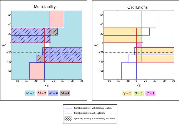
Figure 6: An example of codimension two bifurcation diagram. This diagram is obtained for a a fully-connected network composed of $N_{\text{E}}=3$ excitatory and $N_{I}=3$ inhibitory neurons. Each excitatory (respectively inhibitory) neuron receives an external stimulus $I_{E}$ (respectively $I_{I}$), while the remaining parameters of the network are reported in Tab. (5). The two panels of the figure refer to the same bifurcation diagram, but have been separated for clarity in order to show how multistability (left panel) and oscillations (right panel) depend on the external stimuli. In more detail, the left panel shows how different combinations of the currents $I_{E,I}$, for this specific network architecture, give rise to a number of stationary solutions $\mathcal{M}$ that ranges from $1$ (monostability) to $4$ (quadristability). Moreover, the right panel shows how, for different values of the stimuli, the network undergoes oscillations with period $\mathcal{T}=2$, $3$ or $4$. The blue lines in the diagram represent the combinations of the current $I_{E,I}$ at which a bifurcation occurs. Here, the stationary states lose their stability, turning into different stationary states or into oscillatory solutions. In a similar way, the red lines represent the bifurcations at which oscillations turn into new oscillations or into stationary solutions. For this reason, some blue and red lines in the diagram overlap. The readers are referred to SubSecs. (S3.1) and (S3.2) of the Supplementary Materials for the derivation of their analytical formulas. The shaded areas represent the regions of the $I_{E}-I_{I}$ plane where the symmetry of the inhibitory neurons is broken, despite the symmetry of the underlying neural equations. This occurs for example with the stationary state $\boldsymbol{\nu}=\left[\begin{array}[t]{cccccc}0&0&0&1&0&0\end{array}\right]^{T}$, since in this case only two inhibitory neurons over three do not fire. On the contrary, in this example the symmetry in the excitatory population is never broken, although this may occur with different network sizes or with different topologies of the synaptic connections. The horizontal dashed line in the panels corresponds to the value of the current to the inhibitory population ($I_{I}=-20$) that we have chosen for the calculation of the codimension one bifurcation diagrams of Fig. (7).

$\boldsymbol{\theta}=\left[\begin{array}[]{c}1\\ \vdots\\ 1\end{array}\right],\quad J=\left[\begin{array}[]{cc}\mathfrak{J}_{EE}&\mathfrak{J}_{EI}\\ \mathfrak{J}_{IE}&\mathfrak{J}_{II}\end{array}\right],\quad\mathfrak{J}_{\alpha\alpha}=J_{\alpha\alpha}\left[\begin{array}[]{ccc}0&1&1\\ 1&0&1\\ 1&1&0\end{array}\right],\quad\mathfrak{J}_{\alpha\beta}=J_{\alpha\beta}\left[\begin{array}[]{ccc}1&1&1\\ 1&1&1\\ 1&1&1\end{array}\right]\;\mathrm{for}\;\alpha\neq\beta$

$J_{EE}=-J_{II}=80,\quad J_{IE}=-J_{EI}=70$

Table 5: Set of parameters used for generating Figs. (6) and (7).

The codimension one bifurcation diagrams can be derived analytically from Eq. (1) for $\sigma_{i}^{\mathcal{B}}=0$, by replacing the firing rates of the stationary solutions or those of the oscillatory solutions, and then by calculating $V$ as a function of the stimuli. More explicitly, in our example of a fully-connected network we obtain:

$$\begin{cases}V_{E}\left(I_{E},I_{I}\right)=\frac{N_{E}-1}{N-1}J_{EE}\nu_{E}\left(I_{E},I_{I}\right)+\frac{J_{EI}}{N-1}\sum_{j=0}^{N_{I}-1}\nu_{I,j}\left(I_{E},I_{I}\right)+I_{E}\vphantom{{\displaystyle\sum_{\begin{subarray}{c}j=0\\ j\neq i\end{subarray}}^{N_{I}-1}}}\\ V_{I,i}\left(I_{E},I_{I}\right)=\frac{N_{E}}{N-1}J_{IE}\nu_{E}\left(I_{E},I_{I}\right)+\frac{J_{II}}{N-1}{\displaystyle\sum_{\begin{subarray}{c}j=0\\ j\neq i\end{subarray}}^{N_{I}-1}}\nu_{I,j}\left(I_{E},I_{I}\right)+I_{I},\quad i=0,1,2,\end{cases}$$ (11)

where $V_{E}\left(I_{E},I_{I}\right)$ and $V_{I,i}\left(I_{E},I_{I}\right)$ represent the (stimulus-dependent) membrane potentials in the excitatory and inhibitory population, respectively. Moreover, $\nu_{E}\left(I_{E},I_{I}\right)$ and $\nu_{I,i}\left(I_{E},I_{I}\right)$ are the excitatory and inhibitory firing rates of the stationary/oscillatory solutions, that we obtained numerically as described above. The relation between $\nu_{E,I}$ and $I_{E,I}$ is calculated analytically in Sec. (S3) of the Supplementary Materials. In particular, we observe that in the excitatory population the stationary firing rates (namely the three top entries of the binary representation of the states $0-7$ and $56-63$) and the corresponding membrane potentials are homogeneous ($\nu_{i}=\nu_{E}\left(I_{E},I_{I}\right)$ and $V_{i}=V_{E}\left(I_{E},I_{I}\right)$ for $i=0,1,2$), while in the inhibitory population they are generally heterogeneous ($\nu_{N_{I}+i}=\nu_{I,i}$ and $V_{N_{I}+i}=V_{I,i}\left(I_{E},I_{I}\right)$ for $i=0,1,2$). This is an example of symmetry-breaking that occurs in the inhibitory population (see the shaded areas in the left panel of Fig. (6)). On the contrary, according to the numerical solutions there is no symmetry-breaking during the oscillatory dynamics (see the right panel of Fig. (6)), therefore in this case the firing rates are homogeneous in both the neural populations. Eq. (11) is plotted in the top panels of Fig. (7).

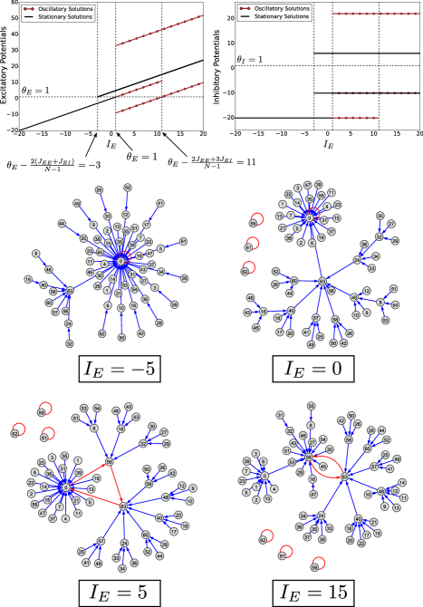
Figure 7: Examples of codimension one bifurcation diagrams. This figure is obtained in the case of the fully-connected network discussed in SubSec. (3.3), for $I_{I}=-20$ (see the horizontal dashed line in Fig. (6)). The top panels represent the codimension one bifurcation diagrams of the excitatory (left) and inhibitory (right) neurons, obtained from Eq. (11) as a function of the stimulus $I_{E}$. In particular, from the firing rates $\nu_{E}$ and $\nu_{I,j}$ of the stationary states, Eq. (11) provides the fixed point solutions of the membrane potentials (black lines). In a similar way, from the firing rates of the oscillatory states we obtain the fixed point cycle solutions (brown lines). The remaining panels of the figure show all the possible bifurcations of the firing rates, for increasing $I_{E}$. The graphs have been obtained from Eq. (10), and highlight in red all the stationary and oscillatory solutions of the network dynamics (compare with the areas crossed by the dashed line in Fig. (6) when moving from left to right).

3.4 Higher-Order Cross-Correlations

The study of correlations among neurons is a topic of central importance to systems neuroscience. Second-order and higher-order correlations are key to understanding the information encoding capabilities of neural populations [1, 30, 29, 5, 25] and to making inferences about how neurons exchange and integrate information [35, 37, 7, 32, 16].

In [14] the authors introduced the following normalized coefficient for quantifying the higher-order correlations among an arbitrary number $n$ of neurons (groupwise correlation) in a network of size $N$ (with $2\leq n\leq N$):

$$\mathrm{Corr}_{n}\left(x_{i_{0}}\left(t\right),\ldots,x_{i_{n-1}}\left(t\right)\right)=\frac{\overline{\prod_{m=0}^{n-1}\left(x_{i_{m}}\left(t\right)-\overline{x}_{i_{m}}\left(t\right)\right)}}{\sqrt[n]{\prod_{m=0}^{n-1}\overline{\left|x_{i_{m}}\left(t\right)-\overline{x}_{i_{m}}\left(t\right)\right|^{n}}}}.$$ (12)

The bar represents the statistical mean over trials computed at time $t$. The variables $x$ in Eq. (12) can be either the membrane potentials or the firing rates. In the first case, in SubSec. (4.1) of the Supplementary Materials we prove that in the stationary regime:

$$\mathrm{Corr}_{n}\left(V_{i_{0}}\left(t\right),\ldots,V_{i_{n-1}}\left(t\right)\right)= \frac{\sqrt{\pi}\sum_{j=0}^{2^{N}-1}F_{j}\prod_{m=0}^{n-1}\mathcal{R}_{j,i_{m}}^{\left(N\right)}}{2^{\frac{n}{2}}\Gamma\left(\frac{n+1}{2}\right)\sqrt[n]{\prod_{m=0}^{n-1}\left[\left(\sigma_{i_{m}}^{\mathcal{B}}\right)^{n}\sum_{j=0}^{2^{N}-1}F_{j}\Phi\left(-\frac{n}{2},\frac{1}{2};-\frac{1}{2}\left(\frac{\mathcal{R}_{j,i_{m}}^{\left(N\right)}}{\sigma_{i_{m}}^{\mathcal{B}}}\right)^{2}\right)\right]}}$$

$$\mathcal{R}_{j,i_{m}}^{\left(N\right)}= \frac{1}{M_{i_{m}}}\sum_{l=0}^{N-1}\left[\left(\mathscr{B}_{j,l}^{\left(N\right)}-\sum_{k=0}^{2^{N}-1}F_{k}\mathscr{B}_{k,l}^{\left(N\right)}\right)J_{i_{m}l}\right],$$

where $\Gamma$ and $\Phi$ are the gamma function and Kummer’s confluent hypergeometric function of the first kind, respectively. Moreover, in SubSec. (S4.2) of the Supplementary Materials we prove that the higher-order correlation structure of the firing rates is given by the following formula:

$$\mathrm{Corr}_{n}\left(\nu_{i_{0}}\left(t\right),\ldots,\nu_{i_{n-1}}\left(t\right)\right)= \frac{\sum_{j=0}^{2^{N}-1}F_{j}\prod_{m=0}^{n-1}\left(1-2\overline{\nu}_{i_{m}}-E_{j,i_{m}}\right)}{2^{n}\sqrt[n]{\prod_{m=0}^{n-1}Z_{n}\left(\overline{\nu}_{i_{m}}\right)}}$$

$$Z_{n}\left(x\right)= x^{n}\left(1-x\right)+x\left(1-x\right)^{n}$$

$$\overline{\nu}_{i_{m}}= \frac{1}{2}\left(1-\sum_{j=0}^{2^{N}-1}F_{j}E_{j,i_{m}}\right)$$

$$E_{j,i_{m}}= \mathrm{erf}\left(\frac{\theta_{i_{m}}-\frac{1}{M_{i_{m}}}\sum_{l=0}^{N-1}J_{i_{m}l}\mathscr{B}_{j,l}^{\left(N\right)}-I_{i_{m}}}{\sqrt{2}\sigma_{i_{m}}^{\mathcal{B}}}\right).$$

In Fig. (8) we show an example of cross-correlations between pairs of neurons (i.e. $n=2$, in which case Eq. (12) corresponds to the Pearson’s correlation coefficient). In the same figure we also show the corresponding standard deviations of the membrane potentials and the firing rates:

$$\sigma_{i}^{V}= \sqrt{\left(\sigma_{i}^{\mathcal{B}}\right)^{2}+\sum_{m=0}^{2^{N}-1}F_{m}\left(\mathcal{R}_{m,i}^{\left(N\right)}\right)^{2}}$$

$$\sigma_{i}^{\nu}= \sqrt{\overline{\nu}_{i}-\left(\overline{\nu}_{i}\right)^{2}}$$

(derived in Eqs. (S29) and (S33) of the Supplementary Materials).

Figure 8: An example of cross-correlation structure for $\boldsymbol{N=4}$. This figure is obtained for the values of the parameters in Tab. (6). The top-panels show the comparison between the analytical standard deviations (given by Eq. (LABEL:eq:standard-deviations), for $I\in\left[-12,12\right]$) of the membrane potentials (left) and the firing rates (right), and the corresponding numerical approximations. For each value of the stimulus $I$, we calculated the network statistics through a Monte Carlo method over $10^{5}$ repetitions. The middle panels show the same comparison for the cross-correlations between neurons $0$ and $1$ (the red curves are described by Eqs. (LABEL:eq:higher-order-correlations-of-the-memebrane-potentials), left, and (LABEL:eq:higher-order-correlations-of-the-firing-rates), right). The bottom panels show examples of highly correlated activity (synchronous states) between the membrane potentials (for $I=0$, left) and between the firing rates (for $I=2$, right).

$J=\left[\begin{array}[]{cccc}0&-15&45&-120\\ 15&0&90&-285\\ 90&-105&0&-3\\ 165&-60&75&0\end{array}\right],\quad\boldsymbol{I}=I\left[\begin{array}[]{c}1\\ 1\\ 1\\ 1\end{array}\right],\quad\boldsymbol{\sigma}=\left[\begin{array}[]{c}1\\ 3\\ 2\\ 2\end{array}\right]$

Table 6: Set of parameters used for generating Fig. (8). The values of the stimulus $I$ are specified in the figure.

Examples of cross-correlations for $n>2$ are shown in Fig. (S3) of the Supplementary Materials. Our analysis shows that the external stimulus $I$ dynamically switches the network between synchronous (i.e. highly correlated) and asynchronous (i.e. uncorrelated) states. The conditions under which these states may occur are discussed in SubSecs. (S4.1.1), (S4.1.2) and (S4.2.1) of the Supplementary Materials. In general, we did not observe any relation between $\mathrm{Corr}_{n}\left(V_{i_{0}}\left(t\right),\ldots,V_{i_{n-1}}\left(t\right)\right)$ and $\mathrm{Corr}_{n}\left(\nu_{i_{0}}\left(t\right),\ldots,\nu_{i_{n-1}}\left(t\right)\right)$, so that low (respectively high) correlations between the membrane potentials do not necessarily correspond to low (respectively high) correlations between the firing rates.

3.5 Mean-Field Limit

In this section we study Eq. (1) in the thermodynamic limit $N\rightarrow\infty$ by means of Sznitman’s mean-field theory (see [38, 2] and references therein). As discussed in [14], generally Sznitman’s theory can be applied only to networks with sufficiently dense synaptic connections. For this reason, we suppose that the network is composed of $\mathfrak{P}$ neural populations $\alpha$ (for $\alpha=0,\ldots,\mathfrak{P}-1$), and that within each population the neurons have fully-connected topology and homogeneous parameters. From this assumption it follows for example that the stimuli are organized into $\mathfrak{P}$ vectors $\boldsymbol{I}_{\alpha}$, one to each population, and such that:

$$\boldsymbol{I}_{\alpha}\left(t\right)=I_{\alpha}\left(t\right)\boldsymbol{1}_{N_{\alpha}},$$ (16)

where $\boldsymbol{1}_{N_{\alpha}}$ is the $N_{\alpha}\times 1$ all-ones vector and $N_{\alpha}$ is the size of the population $\alpha$. In a similar way, the synaptic connectivity matrix can be written as follows:

$$\begin{array}[]{ccc}J=\left[\begin{array}[]{cccc}\mathfrak{J}_{00}&\mathfrak{J}_{01}&\cdots&\mathfrak{J}_{0,\mathfrak{P}-1}\\ \mathfrak{J}_{10}&\mathfrak{J}_{11}&\cdots&\mathfrak{J}_{1,\mathfrak{P}-1}\\ \vdots&\vdots&\ddots&\vdots\\ \mathfrak{J}_{\mathfrak{P}-1,0}&\mathfrak{J}_{\mathfrak{P}-1,1}&\cdots&\mathfrak{J}_{\mathfrak{P}-1,\mathfrak{P}-1}\end{array}\right],&&\mathfrak{J}_{\alpha\beta}=\begin{cases}J_{\alpha\alpha}\left(\mathbb{I}_{N_{\alpha}}-\mathrm{Id}_{N_{\alpha}}\right),&\;\mathrm{for}\;\alpha=\beta\\ \\ J_{\alpha\beta}\mathbb{I}_{N_{\alpha},N_{\beta}},&\;\mathrm{for}\;\alpha\neq\beta\end{cases}\end{array}$$ (17)

for $\alpha,\beta=0,\ldots,\mathfrak{P}-1$. The real numbers $J_{\alpha\beta}$ are free parameters that describe the strength of the synaptic connections from the population $\beta$ to the population $\alpha$. Moreover, $\mathbb{I}_{N_{\alpha},N_{\beta}}$ is the $N_{\alpha}\times N_{\beta}$ all-ones matrix (here we use the simplified notation $\mathbb{I}_{N_{\alpha}}\overset{\mathrm{def}}{=}\mathbb{I}_{N_{\alpha},N_{\alpha}}$), while $\mathrm{Id}_{N_{\alpha}}$ is the $N_{\alpha}\times N_{\alpha}$ identity matrix.

In the thermodynamic limit, the neurons become independent and normally distributed, according to the law $V_{i}\left(i\right)\sim\mathcal{N}\left(\overline{V}_{\alpha}\left(t\right),\left(\sigma_{\alpha}^{\mathcal{B}}\right)^{2}\right)$ for every neuron $i$ in population $\alpha$ (see Fig. (9) in the case $\mathfrak{P}=2$). In the mathematical literature, this phenomenon is known as propagation of chaos [38, 2, 14, 13]. As we show in SubSec. (S5.1) of the Supplementary Materials, propagation of chaos allows use to derive the following set of mean-field equations for the mean membrane potentials $\overline{V}_{\alpha}$ :

$$\overline{V}_{\alpha}\left(t+1\right)=\frac{1}{2}\sum_{\beta=0}^{\mathfrak{P}-1}R_{\beta}J_{\alpha\beta}\left[1-\mathrm{erf}\left(\frac{\theta_{\beta}-\overline{V}_{\beta}\left(t\right)}{\sqrt{2}\sigma_{\beta}^{\mathcal{B}}}\right)\right]+I_{\alpha}\left(t\right),\;\alpha=0,\ldots,\mathfrak{P}-1,$$ (18)

where $R_{\alpha}=\underset{N\rightarrow\infty}{\lim}\frac{N_{\alpha}}{M_{\alpha}}$. Therefore in the thermodynamic limit the stochastic network model can be reduced to a set of $\mathfrak{P}$ deterministic equations in the unknowns $\overline{V}_{\alpha}$.

Figure 9: Network statistics in the thermodynamic limit. This figure has been obtained for a fully-connected network composed of one excitatory and one inhibitory population, for $N_{E}=N_{I}=\frac{N}{2}$, $I_{E}=-I_{I}=10$ and the values of the parameters reported in Tab. (7). The top panels show the fast convergence of the single-neuron marginal probability distributions of the membrane potentials to the mean-field normal distribution $\mathcal{N}\left(\overline{V}_{\alpha}\left(t\right),\left(\sigma_{\alpha}^{\mathcal{B}}\right)^{2}\right)$ for increasing network size $N$ (see text). In particular, the panels show the evolution of the probability distribution of the excitatory neurons, but this result holds also for the inhibitory population. The bottom panels show the corresponding decrease of the pair-wise correlation between the membrane potentials (left) and the decrease of their distance correlation (right). $\mathrm{Corr}_{\alpha\beta}$ (respectively $\mathrm{dCorr}_{\alpha\beta}$) represents the correlation (respectively the distance correlation) between the membrane potentials of the populations $\alpha$ and $\beta$. In particular, the decrease of the distance correlation with the network size numerically proves that the neurons become increasingly independent in the thermodynamic limit [36]. In the mathematical literature, this phenomenon is known as propagation of chaos [38, 2, 14, 13], and represents a key property of the network that allows us to derive its mean-field equations (18). In this figure, for each value of $N$ we calculated the numerical probability distributions, the correlations and the distance correlations through a Monte Carlo method over $10^{4}$ repetitions, so that the statistical error is of the order of $10^{-2}$.

$J_{EE}=-J_{II}=80,$	$\theta_{E}=\theta_{I}=1$
$J_{IE}=-J_{EI}=70,$	$\sigma_{E}^{\mathcal{B}}=1,\;\sigma_{I}^{\mathcal{B}}=2$

Table 7: Set of parameters used for generating Fig. (9) and the top panels of Fig. (10).

We observe that, unlike the original network equations (1), the activation functions in the mean-field equations (18) are differentiable everywhere for $\sigma^{\mathcal{B}}>0$. For this reason, when noise is present in every population, the bifurcation structure of Eq. (18) can be studied through the bifurcation theory of graded systems [22]. For the sake of example, we focus on the case of a network composed of two neural populations, one excitatory and one inhibitory (even though the bifurcation structure may be studied for every $\mathfrak{P}$). From now on, it is convenient to change slightly the notation, and to consider $\alpha=E,\,I$ rather than $\alpha=0,\,1$. Beyond global bifurcations, which generally cannot be studied analytically, the mean-field network may undergo limit-point, period-doubling and Neimark-Sacker local bifurcations. By applying the technique developed in [19, 12], in SubSec. (S5.2) of the Supplementary Materials we prove that these local codimension one bifurcations are analytically described by the following set of parametric equations:

$$\begin{cases}I_{E}\left(\mathfrak{v}\right)=\mathfrak{v}-\frac{1}{2}R_{E}J_{EE}\left[1+\mathrm{erf}\left(\frac{\mathfrak{v}-\theta_{E}}{\sqrt{2}\sigma_{E}^{\mathcal{B}}}\right)\right]-\frac{1}{2}R_{I}J_{EI}\left[1+\mathrm{erf}\left(\frac{\mu_{I}\left(\mathfrak{v}\right)-\theta_{I}}{\sqrt{2}\sigma_{I}^{\mathcal{B}}}\right)\right]\\ \\ I_{I}\left(\mathfrak{v}\right)=\mu_{I}\left(\mathfrak{v}\right)-\frac{1}{2}R_{E}J_{IE}\left[1+\mathrm{erf}\left(\frac{\mathfrak{v}-\theta_{E}}{\sqrt{2}\sigma_{E}^{\mathcal{B}}}\right)\right]-\frac{1}{2}R_{I}J_{II}\left[1+\mathrm{erf}\left(\frac{\mu_{I}\left(\mathfrak{v}\right)-\theta_{I}}{\sqrt{2}\sigma_{I}^{\mathcal{B}}}\right)\right]\end{cases}$$ (19)

in the parameter $\mathfrak{v}$, where:

$$\mu_{I}\left(\mathfrak{v}\right)=\theta_{I}\pm\sqrt{-2\left(\sigma_{I}^{\mathcal{B}}\right)^{2}\ln\left(\sqrt{2\pi}\sigma_{I}^{\mathcal{B}}g_{I}\left(\mu_{I}\right)\right)}.$$

For the limit-point and period-doubling bifurcations we get:

$$g_{I}\left(\mu_{I}\right)=\frac{sR_{E}J_{EE}g_{E}\left(\mathfrak{v}\right)-s^{2}}{R_{E}R_{I}\left(J_{EE}J_{II}-J_{EI}J_{IE}\right)g_{E}\left(\mathfrak{v}\right)-sR_{I}J_{II}},$$

with $s=1$ and $s=-1$ respectively, while for the Neimark-Sacker bifurcation we obtain:

$$g_{I}\left(\mu_{I}\right)=\frac{1}{R_{E}R_{I}\left(J_{EE}J_{II}-J_{EI}J_{IE}\right)g_{E}\left(\mathfrak{v}\right)},$$

where:

$$g_{E}\left(\mathfrak{v}\right)=\frac{1}{\sqrt{2\pi}\sigma_{E}^{\mathcal{B}}}e^{-\frac{\left(\mathfrak{v}-\theta_{E}\right)^{2}}{2\left(\sigma_{E}^{\mathcal{B}}\right)^{2}}}.$$

Eq. (19) describes the local bifurcations in the codimension two bifurcation diagram of the mean-field network. Since global bifurcations cannot be derived analytically, we obtained the complete bifurcation structure of the mean-field network by the MatCont Matlab toolbox [10] (see Fig. (10)).

Figure 10: Bifurcation diagrams of the mean-field model. This figure shows the codimension two (left) and codimension one (right) bifurcation diagrams of the model Eq. (18), obtained numerically by the MatCont Matlab toolbox [10]. In the top panels, which we obtained for $R_{E}=R_{I}=0.5$ and the parameters of Tab. (7), we show the formation of the limit-point ($\mathrm{LP}$) and period-doubling ($\mathrm{PD}$) bifurcations. These local codimension one bifurcations correspond to the blue and red curves in the top-left panel of the figure, and are described analytically by Eq. (19). In this panel we also show the remaining bifurcations of the mean-field model. In particular, the $\mathrm{LPPD}$ bifurcation is a local codimension two bifurcation, which represents the simultaneous occurrence of the limit-point and period-doubling bifurcations. Again, this bifurcation can be described analytically by intersecting the $\mathrm{LP}$ and $\mathrm{PD}$ curves obtained from Eq. (19). Moreover, $\mathrm{LPC}$, $\mathrm{CP}$, $\mathrm{GPD}$ and $\mathrm{R1}$ are limit point of cycles, cusp, generalized period-doubling, and $1:1$ strong resonance bifurcations, respectively. For more details, the reader is referred to [22]. In the top-right panel we show the fixed point curves (black) and the fixed point cycle curves (brown) obtained for $I_{I}=0$, which are mathematically described by Eqs. (S43) and (S52) in the Supplementary Materials, respectively. In the bottom panels, which we obtained for $J_{EE}=-J_{II}=10$, we show the formation of the Neimark-Sacker ($\mathrm{NS}$) bifurcation. This local codimension one bifurcation corresponds to the green curve in the bottom-left panel of the figure, and is described analytically by Eq. (19). In this panel we also show the formation of Chenciner ($\mathrm{CH}$) and of the $1:\mathrm{X}$ strong resonance bifurcations ($\mathrm{RX}$, for $\mathrm{X}=1,3,4$) [22]. In the bottom-right panel, obtained again for $I_{I}=0$, we omitted the fixed point cycle curve from our analysis because of its high complexity. This curve may be calculated numerically as explained in SubSec. (S5.2.3) of the Supplementary Materials, if desired.

4 Discussion

We studied a synchronously updated firing-rate neural network model with asymmetric synaptic weights and discrete-time evolution, that allows exact analytical solutions for any network size $N$. The main difficulty in studying asymmetric neural networks is the impossibility to apply the powerful methods of equilibrium statistical mechanics, because no energy function exists for these networks. For this reason, exactly solvable neural network models with asymmetric weights are still rare [20, 6, 31, 9, 39]. Exact analytical solutions are available only in some mean-field approaches, such as the limit of an infinite number of spin components, or the thermodynamic limit of infinite network size. On the contrary, our model allows exact solutions for any network size $N$. This is due to the use of the stochastic recurrence relation (1), rather than Little’s definition of temperature [23] (in particular, compare our Eq. (8) with Little’s Eq. (4)). In this respect, our work follows the approach described in [39], but with some important differences. In [39] the authors specifically considered first- and second-order Hebbian synaptic connections in a diluted network with Gaussian noise, and studied the dynamical evolution of the overlap between the state of the network and the stored point attractors in the thermodynamic limit. On the contrary, in our work we considered first-order synaptic connections with an arbitrary synaptic matrix $J$ and arbitrary noise statistics, and we derived exact solutions for any network size $N$ without further assumptions, as described below.

In particular, we derived exact solutions for the conditional probability distributions of the membrane potentials and the firing rates, as well as for the joint probability distributions in the stationary regime. Due to the asymmetry of the synaptic weights, the network we studied can undergo oscillations with period $\mathcal{T}\geq 2$, while synchronous Hopfield networks (which have symmetric connections) can sustain only oscillations with period $\mathcal{T}=2$, known as two-cycles [17]. Moreover, compared to small-size graded networks [14, 13], where the impossibility to use statistical methods restricts the derivation of (approximate) analytical formulas of the joint probability distributions only to simple network topologies, here we derived an exact solution which is valid for any connectivity matrix $J$.

The formula of the conditional probability distribution of the firing rates allowed us to define a new learning rule to store point and periodic attractors. Point attractors correspond to stable states, while periodic attractors represent oscillatory solutions of the network activity. The learning rule that we introduced can be seen as a variant of the so called pseudoinverse learning rule for discrete-time systems [40]. While the pseudoinverse rule was introduced in [28] for deterministic Hopfield-type models, our rule can also be used to safely store sequences of activity patterns in noisy networks.

To complete our analysis on the formation of stable and oscillatory solutions, we performed an analytical study of the bifurcations. The method we proposed can be applied to networks with any topology, but for the sake of example, we considered the case of a fully-connected network. As is common practice, we performed the bifurcation analysis in the zero-noise limit $\sigma^{\mathcal{B}}\rightarrow 0$. We derived analytical expressions for the codimension one and codimension two bifurcation diagrams, showing how the external stimuli affect the neuronal dynamics. It is important to observe that in graded networks the local bifurcations are studied through the eigenvalues of the Jacobian matrix of the network equations [12], which are not defined in our model due to the discontinuous activation function (2). For this reason, we took advantage of the conditional probability distribution of the firing rates, which allowed us to determine for which combinations of the external stimuli the network undergoes multistability, oscillations or symmetry-breaking.

Then, we derived exact expressions of the higher-order correlation structure of noisy networks in the stationary regime, for both the membrane potentials and the firing rates. In the case of the time-continuous graded networks studied in [14, 13], the authors found analytical (approximate) solutions of the correlation structure through a perturbation analysis of the neural equations in the small-noise limit $\sigma^{\mathcal{B}}\ll 1$. A consequence of this approximation is that the correlations between the membrane potentials and those between the firing rates have the same mathematical expression in the graded model. On the contrary, in this article we derived exact expressions of the correlations for any noise intensity. Due to the discontinuous activation function (2), the two correlations structures are never identical, even in the small-noise limit. Moreover, similarly to the case of graded networks [13], we found that the external stimuli can dynamically switch the neural activity from asynchronous (i.e. uncorrelated) to synchronous (i.e. highly correlated) states, with two important differences. The first is that low (respectively high) correlations between the membrane potentials do not necessarily correspond to low (respectively high) correlations between the firing rates. The second is that while in graded networks synchronous states may occur through critical slowing down [13], the discrete network considered here relies on different mechanisms for generating highly correlated activity, that we have only partially covered. Indeed critical slowing down is deeply related to the eigenvalues of the network, which are not defined for a system with discontinuous activation function like ours.

For completeness and in order to link our results to previous work on asymmetric models, we derived the mean-field equations of the network in the thermodynamic limit $N\rightarrow\infty$. Due to the limitations of Sznitman’s mean-field theory, we derived these equations only for sufficiently dense multi-population networks driven by independent sources of noise. Then, by applying the methods developed in [19, 12], we derived exact analytical expressions for the local codimension one bifurcations in terms of the external stimuli. This method can be applied to networks composed of an arbitrary number of populations, but for the sake of example we considered the simple case of two populations. This allowed us to describe analytically part of the codimension two bifurcation diagram of the network, while we found the global bifurcations numerically by the MatCont Matlab toolbox [10].

To conclude, we observe that solvable finite-size network models are invaluable theoretical tools for studying the brain at its multiple scales of spatial organization. Studying how the complexity of neuronal activity changes for increasing network size is of fundamental importance for unveiling the emergent properties of the brain. In this article, we made an effort in this direction, trying to fill the gap in the current neuroscientific literature. Asymmetric synaptic connections, which are widely considered as a mathematically advanced task, increase the biological plausibility of the model and allows a more complete description of neural oscillations. While we think that these results are of considerable theoretical interest by themselves, in future work we will rigorously determine how the two main assumptions of the model, namely the discrete-time evolution and the binary firing rates, affect its capability to describe realistic neuronal activity.

References

- [1] L. F. Abbott and P. Dayan. The effect of correlated variability on the accuracy of a population code. Neural Comput., 11(1):91–101, 1999.
- [2] J. Baladron, D. Fasoli, O. Faugeras, and J. Touboul. Mean-field description and propagation of chaos in networks of Hodgkin-Huxley and FitzHugh-Nagumo neurons. J. Math. Neurosci., 2(1):10, 2012.
- [3] R. M. Borisyuk and A. B. Kirillov. Bifurcation analysis of a neural network model. Biol. Cybern., 66(4):319–325, 1992.
- [4] A. Bovier and P. Picco. Mathematical aspects of spin glasses and neural networks. Progress in Probability. Birkhäuser Boston, 2012.
- [5] M. R. Cohen and J. H. Maunsell. Attention improves performance primarily by reducing interneuronal correlations. Nature Neurosci., 12(12):1594–1600, 2009.
- [6] A. Crisanti and H. Sompolinsky. Dynamics of spin systems with randomly asymmetric bonds: Langevin dynamics and a spherical model. Phys. Rev. A, 36:4922–4939, 1987.
- [7] O. David, D. Cosmelli, and K. J. Friston. Evaluation of different measures of functional connectivity using a neural mass model. NeuroImage, 21(2):659–673, 2004.
- [8] J. DeFelipe, P. Marco, I. Busturia, and A. Merchán-Pérez. Estimation of the number of synapses in the cerebral cortex: Methodological considerations. Cereb. Cortex, 9(7):722, 1999.
- [9] B. Derrida, E. Gardner, and A. Zippelius. An exactly solvable asymmetric neural network model. Europhys. Lett., 4(2):167–173, 1987.
- [10] A. Dhooge, W. Govaerts, and Y. A. Kuznetsov. MATCONT: A MATLAB package for numerical bifurcation analysis of ODEs. ACM Trans. Math. Softw., 29(2):141–164, 2003.
- [11] B. Ermentrout. Neural networks as spatio-temporal pattern-forming systems. Rep. Prog. Phys., 61(4):353–430, 1998.
- [12] D. Fasoli, A. Cattani, and S. Panzeri. The complexity of dynamics in small neural circuits. PLoS Comput. Biol., 12(8):1–35, 2016.
- [13] D. Fasoli, A. Cattani, and S. Panzeri. From local chaos to critical slowing down: A theory of the functional connectivity of small neural circuits. arXiv:1605.07383 [q-bio.NC], 2016.
- [14] D. Fasoli, O. Faugeras, and S. Panzeri. A formalism for evaluating analytically the cross-correlation structure of a firing-rate network model. JMN, 5:6, 2015.
- [15] W. Feller. An introduction to probability theory and its applications, volume 1. John Wiley, New York, 1971.
- [16] K. J. Friston. Functional and effective connectivity: A review. Brain Connect., 1(1):13–36, 2011.
- [17] E. Goles-Chacc, F. Fogelman-Soulie, and D. Pellegrin. Decreasing energy functions as a tool for studying threshold networks. Discrete Appl. Math., 12(3):261–277, 1985.
- [18] F. Grimbert and O. Faugeras. Bifurcation analysis of Jansen’s neural mass model. Neural Comput., 18(12):3052–3068, 2006.
- [19] R. Haschke and J. J. Steil. Input space bifurcation manifolds of recurrent neural networks. Neurocomputing, 64:25–38, 2005.
- [20] J. A. Hertz, G. Grinstein, and S. A. Solla. Irreversible spin glasses and neural networks, pages 538–546. Springer Berlin Heidelberg, 1987.
- [21] J. J. Hopfield. Neural networks and physical systems with emergent collective computational abilities. PNAS, 79(8):2554–2558, 1982.
- [22] Y. A. Kuznetsov. Elements of applied bifurcation theory, volume 112. Springer-Verlag New York, 1998.
- [23] W. A. Little. The existence of persistent states in the brain. Math. Biosci., 19(1):101–120, 1974.
- [24] W. McCulloch and W. Pitts. A logical calculus of the ideas immanent in nervous activity. Bull. Math. Biophys., 5:115–133, 1943.
- [25] R. Moreno-Bote, J. Beck, I. Kanitscheider, X. Pitkow, P. Latham, and A. Pouget. Information-limiting correlations. Nature Neurosci., 17(10):1410–1417, 2014.
- [26] T. Morita and T. Horiguchi. Exactly solvable model of a spin glass. Solid State Commun., 19(9):833–835, 1976.
- [27] P. Peretto. Collective properties of neural networks: A statistical physics approach. Biol. Cybern., 50(1):51–62, 1984.
- [28] L. Personnaz, I. Guyon, and G. Dreyfus. Collective computational properties of neural networks: New learning mechanisms. Phys. Rev. A, 34(5):4217–4228, 1986.
- [29] J. W. Pillow, J. Shlens, L. Paninski, A Sher, A. M. Litke, E. J. Chichilnisky, and E. P. Simoncelli. Spatio-temporal correlations and visual signaling in a complete neuronal population. Nature, 454(7206):995–999, 2008.
- [30] G. Pola, A. Thiele, K. P. Hoffmann, and S. Panzeri. An exact method to quantify the information transmitted by different mechanisms of correlational coding. Network: Comput. Neural Syst., 14(1):35–60, 2003.
- [31] H. Rieger, M. Schreckenberg, and J. Zittartz. Glauber dynamics of neural network models. J. Phys. A: Math. Gen., 21(4):L263, 1988.
- [32] B. P. Rogers, V. L. Morgan, A. T. Newton, and J. C. Gore. Assessing functional connectivity in the human brain by fmri. Magn. Reson. Imaging, 25(10):1347–1357, 2007.
- [33] F. Rosenblatt. The perceptron: A probabilistic model for information storage and organization in the brain. Psychol. Rev., 65(6):386–408, 1958.
- [34] D. Sherrington and S. Kirkpatrick. Solvable model of a spin-glass. Phys. Rev. Lett., 35:1792–1796, 1976.
- [35] W. Singer. Synchronization of cortical activity and its putative role in information processing and learning. Annu. Rev. Physiol., 55(1):349–374, 1993.
- [36] G. J. Székely, M. L. Rizzo, and N. K. Bakirov. Measuring and testing dependence by correlation of distances. Ann. Stat., 35(6):2769–2794, 2007.
- [37] G. Tononi, O. Sporns, and G. M. Edelman. A measure for brain complexity: relating functional segregation and integration in the nervous system. Proc. Natl. Acad. Sci. U.S.A., 91(11):5033–5037, 1994.
- [38] J. Touboul, G. Hermann, and O. Faugeras. Noise-induced behaviors in neural mean field dynamics. SIAM J. Appl. Dyn. Syst., 11(1):49–81, 2012.
- [39] L. Wang, E. E. Pichler, and J. Ross. Oscillations and chaos in neural networks: An exactly solvable model. PNAS, 87(23):9467–9471, 1990.
- [40] C. Zhang, G. Dangelmayr, and I. Oprea. Storing cycles in Hopfield-type networks with pseudoinverse learning rule: Admissibility and network topology. Neural Networks, 46:283–298, 2013.