Three dimensional boundary displacement due to stable ideal kink modes excited by external n=2 magnetic perturbations

Abstract

In low- collisionality ($\nu^{\star}$) scenarios exhibiting mitigation of edge localized modes, stable ideal kink modes at the edge are excited by externally applied magnetic perturbation (MP)-fields. At ASDEX Upgrade these modes can cause three-dimensional (3D) boundary displacements up to the centimeter range. These displacements have been measured using toroidally localized high resolution diagnostics and rigidly rotating $n=2$ MP-fields with various applied poloidal mode spectra. These measurements are compared to non-linear 3D ideal magnetohydrodynamics (MHD) equilibria calculated by VMEC. Comprehensive comparisons have been conducted, which consider for instance plasma movements due to the position control system, attenuation due to internal conductors and changes in the edge pressure profiles.

VMEC accurately reproduces the amplitude of the displacement and its dependencies on the applied poloidal mode spectra. Quantitative agreement is found around the low field side (LFS) midplane. The response at the plasma top is qualitatively compared. The measured and predicted displacements at the plasma top maximize when the applied spectra is optimized for ELM-mitigation. The predictions from the vacuum modeling generally fails to describe the displacement at the LFS midplane as well as at the plasma top. When the applied mode spectra is set to maximize the displacement, VMEC and the measurements clearly surpass the predictions from the vacuum modeling by a factor of four. Minor disagreements between VMEC and the measurements are discussed. This study underlines the importance of the stable ideal kink modes at the edge for the 3D boundary displacement in scenarios relevant for ELM-mitigation.

1 Introduction

Externally applied MPs can be used to mitigate and to suppress ELMs in high confinement mode (H-mode) [1]. At low collisionality ($\acs{nustar}<0.3$), ELM mitigation and suppression are accompanied with a loss of confinement primarily resulting in the loss of density, the so-called density ’pump-out’. Recent studies at ASDEX Upgrade [2, 3], DIII-D [4] and MAST [2] have shown that both the best ELM mitigation as well as suppression are achieved by an externally applied MP-field when its poloidal mode spectrum excites modes at the edge which are most amplified by the plasma. According to MHD calculations [5], these modes are stable ideal kink modes, which are driven by the H-mode edge pressure gradient and/or the associated bootstrap current [6]. Because of the amplification by the plasma, the resulting MPs at the plasma boundary can be even larger than expected solely from the externally applied MPs [7, 8]. Moreover, these stable kink modes cause a 3D displacement of the plasma boundary, which is clamped to the applied MP field. MHD codes, like IPEC [9], JOREK [10], MARS-F [11], M3D-C1 [12], VMEC [13, 14] are able to calculate this deformation for various plasma scenarios and coil configurations. These MHD codes predict that the X-point displacement, also referred as high field side (HFS) response [6] or peeling response, maximizes when the applied poloidal mode spectrum is optimized for ELM mitigation or suppression. It is therefore assumed that the X-point displacement influences the ELM stability.

The characterization and prediction of the non-axisymmetric boundary deformation is important because such 3D geometry can influence the ELM stability [15], turbulent transport [16] and the coupling of the ion cyclotron resonance heating (ICRH) [17]. The 3D boundary distortion from external MPs has been extensively studied in various machines like ASDEX Upgrade [18, 19], DIII-D [20, 7, 12], MAST [21], JET [22, 23] and has been reviewed in Ref. [24]. The main conclusion of Ref. [24] is that the measured displacement of the LFS midplane boundary depends approximately linearly on the applied resonant field predicted by vacuum field modeling [24]. But it was also observed that in some cases the vacuum modeling clearly underestimates the displacement due to stable ideal kink modes.

In this paper, we demonstrate that in a scenario which exhibits ELM mitigation at low $\nu^{\star}$ stable ideal kink modes dominate the boundary displacement. When the applied poloidal mode spectrum is optimized to excite the edge kink mode, the displacement is about four times larger than the expectation from the vacuum field modeling. Thus, predictions by vacuum field modeling are not a good approximation. This is similar to one case studied in Ref. [7, 25]. We extended the analysis of Ref. [26] and present comprehensive studies of the 3D boundary displacement at ASDEX Upgrade using rigidly rotating MP-fields with toroidal mode number $n=2$ and toroidally localized diagnostics. The analysis methods have been further improved including the effects from the plasma position control system, the attenuation of the MP-field from internal conductors and the applied poloidal mode spectrum. This allows us to achieve a new level of accuracy and to perform detailed analyses of the local plasma response via the displacement. We further characterize the dependence of the 3D displacement on the applied poloidal mode spectra by varying the differential phase angle ($\Delta\varphi\rm{{}_{UL}}$) [27], which is the toroidal phase of the MP-field from the upper coil set $\varphi\rm{{}_{U}}$ subtracted by the lower one $\varphi\rm{{}_{L}}$, $\acs{dphi}=\varphi\rm{{}_{U}}-\varphi\rm{{}_{L}}$. These measurements are compared to the results of the non-linear ideal MHD equilibrium code VMEC, which has also been employed at other devices [21, 28, 29, 30]. It is demonstrated that VMEC can predict quantitatively the displacement.

This paper is organized as follows. Section 2 describes the experimental configuration and measuring principles. The modeling is described in section 3. In section 4, we test the plasma response via the ELM behavior. This is then compared to displacement measurements and calculations around the plasma top in section  5. The comparison between measurements and modeling of the displacement around the LFS midplane is shown in section 6. This paper concludes with section 7. The sensitivity studies regarding the grid resolution in VMEC are shown in the Appendix.

2 Experimental configuration

2.1 Discharge configuration with rigid rotations

The present configuration is very similar to the one studied in Ref. [26]. The experiments have a toroidal field $B\rm{{}_{T}}$ of $-2.5\ \rm{T}$, low triangularity (lower $\delta\rm{{}_{l}}=0.52$ and upper $\delta\rm{{}_{u}}=0.119$) and a plasma current of $800\ \rm{kA}$ resulting in a safety factor of $q_{95}\approx-5.2$. In addition to the ohmic heating of about $300\;\rm{kW}$, the external heating power in the discharges presented here amounts to around $7\;\rm{MW}$ from neutral beam injection (NBI) and $2\;\rm{MW}$ from centrally deposited electron cyclotron resonance heating (ECRH).

The applied $n=2$ MP-fields are produced by 16 saddle coils with 8 coils in each row (see Ref. [27]). To measure the displacement using toroidally localized diagnostics, we rotate the applied MP-field rigidly. Figure 1 shows time traces of a typical discharge. To indicate the timing of the rigid rotation, the top frame shows the supplied current of one MP-coil. To test the plasma response for different applied poloidal mode spectra, we varied $\Delta\varphi\rm{{}_{UL}}$ in-between discharges and, in some cases, during the discharge. In the illustrated discharge, the external MP-field rotates rigidly with $2\;\rm{Hz}$ at two different values for $\Delta\varphi\rm{{}_{UL}}$ for 3 seconds each. First, $\Delta\varphi\rm{{}_{UL}}$ of $\approx 0^{\circ}$ was applied, which is close to the maximum mis-alignment of the external MP-field with respect to the equilibrium field in the pedestal. Therefore, we refer to this configuration as (vacuum) non-resonant in figure 1(b). Then, at 5 seconds, we set $\Delta\varphi\rm{{}_{UL}}$ to $\approx\pm 180^{\circ}$, which is the optimum field-alignment and therefore, labelled as (vacuum) resonant. During both phases a moderate degree of density ’pump-out’ ($10-20\%$) is observed as shown in the measured line integrated densities using the edge and core chord (figure 1(c)). The time trace of one edge electron cyclotron emission (ECE) channel exhibits a clear modulation in the measured radiation temperature ($T\rm{{}_{rad}}$), which is caused by the radial displacement (figure 1(d)). This channel is optically thick, so we can assume that electron temperature ($T\rm{{}_{e}}$) can be approximated by $T\rm{{}_{rad}}$. Furthermore, the amplitude clearly changes with the applied $\Delta\varphi\rm{{}_{UL}}$.

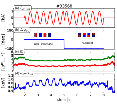
Figure 1: Overview of a typical discharge with rigid rotation: (a) Power supply current of one MP-coil illustrating the timing of the rigid rotation with $2\ \rm{Hz}$, (b) the differential phase angle of two rotation phases employing vacuum non-resonant and resonant configuration, (c) line integrated density of a core (green) and edge chord (red) and (d) $T\rm{{}_{rad}}$($\approx\acs{Te}$) from ECE in the pedestal around the LFS midplane. The modulation amplitude measured by ECE depends clearly on $\Delta\varphi\rm{{}_{UL}}$.

2.2 Set of discharges with rigid rotations

shot	set $\Delta\varphi\rm{{}_{UL}}$ [∘]	f [Hz]	$<\beta_{N}>$	available diagnostics
33118	-90	3	1.82	ECE, CXRS, LIB, REF-X
33345	90 , -90	2	2.18, 1.81	ECE, CXRS, LIB, REF-X
33346	130, 50	2	2.27, 2.09	ECE, CXRS, REF-X
33568	0, $\pm 180$	2	1.83, 1.96	ECE
33569	-50 , -130	2	2.01, 2.03	ECE, CXRS, LIB, REF-X
33570	-100	2	2.0	ECE, CXRS, REF-X

Table 1: Overview of analyzed discharges. The experimental periods used as input for the MHD modeling are colored. $<\beta_{N}>$ is the normalized beta averaged over the analyzed rotation period.

To systematically study the plasma response during ELM mitigation, we applied rigidly rotating MP-fields with various $\Delta\varphi\rm{{}_{UL}}$s. The resulting change of the applied poloidal mode spectra allows us to investigate its impact on the plasma response and the non-axisymmetric boundary displacement. In all discharges, the same plasma shape, heating power and gas fuelling rate was configured. Only in discharge $\#33569$, one gyrotron tripped prior to the rotation phase resulting in $500\ \rm{kW}$ less ECRH power. The set of discharges with the different phases of $\Delta\varphi\rm{{}_{UL}}$ is listed in Table 1. Because the set $\Delta\varphi\rm{{}_{UL}}$ also influences the density ’pump-out’ [4], the density and hence, normalized beta ($\beta\rm{{}_{N}}$) vary by around $20\%$.

2.3 Displacement measurements around the midplane

To measure the radial displacement, we use the high resolution profile diagnostics around the LFS midplane. Figure 2(a) shows the set of used diagnostics consisting of profile ECE [31, 26], lithium beam (LIB) [32, 33], edge charge exchange recombination spectroscopy (CXRS) [34] and X-mode reflectometer (REF-X) [35]. As some diagnostic data were not available for all discharges, the last column of Table 1 lists the availability of the various profile diagnostics.

To determine the displacement around the midplane, we track movements in the profile diagnostics during the rigid rotation using only pre ELM data points ($60-90\%$ of the ELM cycle). In the case of electron density ($n\rm{{}_{e}}$) profile measurements, the procedure is straight forward. We determine the density [26] at the separatrix before the MP-phase and track the position of this values along the diagnostic lines of sight (LOS) during the rigid rotation. In our case, it is $1.2\cdot 10^{19}\ \rm{m^{-3}}$ and is used for all $n\rm{{}_{e}}$ profile diagnostics and for all analyzed phases. Small variations of this density value do not change the outcome of the analysis because of the steep density gradients in the pedestal.

For CXRS measurements a similar method is used. But instead of using the ion temperature ($T\rm{{}_{i}}$) or the rotation profiles, it is more advantageous to use the measured line intensity ($I\rm{{}_{imp}}$), which is Boron 5+ ($B_{5+}$) in this case. $T\rm{{}_{i}}$ and rotation profiles are not reliable in the scrape off layer (SOL), because of a low $I\rm{{}_{imp}}$. They usually exhibit large uncertainties and a large scatter in the SOL (see figure 2(c)). Because of the low beam attenuation at the edge, $I\rm{{}_{imp}}$ is approximately proportional to the impurity density around the plasma boundary. Therefore, the $I\rm{{}_{imp}}$-profile increases monotonically from the SOL towards the pedestal top (figure 2(c)). This allows us to use the same procedure for CXRS as for the $n\rm{{}_{e}}$ profile measurements. A value of $0.5\cdot 10^{17}\ \rm{Ph/m^{2}sr\ s}$ at the separatrix is determined prior to the MP-phase and is used for all cases.

ECE measurements require a different approach due to the non-monotonic behavior of the $T\rm{{}_{rad}}$ profile from the ECE diagnostic at the edge known as the ’shine-through’ effect [31]. To obtain the plasma displacement, first, the $T\rm{{}_{rad}}$ data from the steep gradient region is fitted using a spline at the beginning of each rigid rotation phase [26]. Then, this spline is only varied by a radial shift until the least square (LSQ) is minimized (see also Ref. [26]). This is done for every pre-ELM time point throughout the analyzed time window.

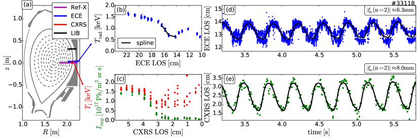
Figure 2: Measuring $\xi_{r}$ around the LFS midplane. (a) poloidal cross-section showing LOS of REF-X, ECE, CXRS and LIB, (b) $T\rm{{}_{rad}}$ profile from ECE and spline (line) to determine profile shift, (c) $T\rm{{}_{i}}$ profile in red and $I\rm{{}_{imp}}$ in green from CXRS. (d) and (e) show time traces of the separatrix position from ECE and CXRS as well as their corresponding sine fits (line), respectively.

2.4 Estimation of the axisymmetric contribution due to the plasma position control

To guarantee a stable plasma operation during these MP-field rotation experiments, the plasma position at the outer midplane is feedback-controlled. The plasma control system (PCS) assumes an axisymmetric equilibrium during the rigidly rotating MP-field. Because the reconstruction of the actual radial plasma position is based on poloidal magnetic field ($B\rm{{}_{\Theta}}$) measurements localized at one toroidal position (blue diamonds in 3(a)), it can induce additional sinusoidal axisymmetric $n=0$ movements of the plasma for two reasons. First, the $B\rm{{}_{\Theta}}$ probes pick up stray-fields from the MP-coils and the field generated by the plasma response to the MP, which are not accounted for in the realtime equilibrium regression used for the PCS. Second, the control system tries to counteract the rotating 3D displacement (see Ref. [36]).

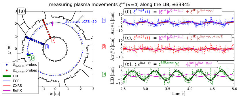
Figure 3: Measuring $n=0$ plasma movements at the LOS of the LIB diagnostic. (a) top view of the experimental configuration showing the various diagnostics and two $B\rm{{}_{\Theta}}$ arrays. Array 1 ($Arr\#1$, blue diamonds), which is used for the PCS and Array 2 ($Arr\#2$, red diamonds). Solid black and dashed blue line indicate the outer LCFS and the displaced VMEC boundary amplified by a factor of 50, respectively. Separatrix movements at the LIB using equilibrium reconstructions with (b) $Arr\#1$ (blue) and (c) $Arr\#2$ (red). The determined axisymmetric $\xi\rm{{}^{axi}}$ and non-axisymmetric contributions $\xi\rm{{}^{3D}}$ are purple and brown, respectively. (d) Measured displacement using LIB (green) and determined displacement (black). In general, effects from PCS are small.

These sinusoidal $n=0$ movements have the same frequency as the rotating displacement and can distort the displacement measurements in amplitude and phase. To interpret the measurements correctly, it is therefore necessary to quantify this contribution from the $n=0$ movements. This can be done by reconstructing the axisymmetric equilibrium throughout the rigid rotation at two toroidal positions using two toroidally separated $B\rm{{}_{\Theta}}$ arrays (blue and red diamonds in figure 3(a)). It allows us to disentangle the $n=0$ movements from distortions in the axisymmetric equilibrium reconstruction due to the non-axisymmetric effects like the 3D displacement and the ’pick-up’ in the magnetic probes. The main idea is that during the rigid rotation the non-axisymmetric contributions appear in both equilibrium reconstructions with a preset phase difference ($n\pi/4$) depending on the toroidal separation of the two probe arrays and the applied toroidal mode number $n$, whereas the axisymmetric $n=0$ contributions appear simultaneously. This enables us to quantify the $n=0$ movements along various LOS of used diagnostics and subtract it from the measured $n=0$ displacement of the LCFS.

One example of this procedure is shown in Figure 3 (discharge $\#33345$, $\acs{dphi}\approx 90^{\circ}$). This experiment exhibits the largest plasma movements ($\pm 1.5\ \rm{mm}$) within the set of discharges (Table 1). Figure 3(b) and (c) show time traces of the separatrix movements along the LIB LOS from the integrated data analysis equilibrium (IDE) [37] data from the array 1 (blue) and array 2 (red), respectively. The determined axisymmetric $n=0$ contribution caused by the control system ($\xi\rm{{}^{axi}}$) and non-axisymmetric one ($\xi\rm{{}^{3D}}$) are shown in purple and brown, respectively. The extracted axisymmetric contribution $\xi\rm{{}^{axi}}$ is then subtracted from the LIB measurement ($\xi\rm{{}^{LIB}}$, green) to determine the actual displacement ($\xi$, black) along the LIB, which is shown in figure 3(d). Please note that the LIB is above the midplane (see figure 2(a)). This procedure is applied to each rigid rotation phase and for each used diagnostics of table 1. In all experiments, the observed $n=0$ movements of the plasma are relatively small ($0-1.5\ \rm{mm}$) with respect to the measured radial displacement ($2-8\ \rm{mm}$). From these numbers, we can already conclude that the PCS in ASDEX Upgrade, which uses only magnetic measurements, is not fully counteracting the 3D boundary displacement [36]. Otherwise, the $n=0$ movements would have the same magnitude as the displacements. Detailed analysis of the behavior of the PCS and the cause of this $n=0$ movements are beyond the scope of this paper and will be published elsewhere.

2.5 Plasma top diagnostics for HFS response

As already mentioned in the introduction, the displacement around the X-point and the HFS response, are thought to be important for ELM mitigation. However, MHD codes with spectral representation exclude the X-point. VMEC calculations done for ASDEX Upgrade plasmas show the lowest displacement amplitude at the X-point. The X-Point region is difficult to diagnose and requires sophisticated plasma response measurements [38]. Instead, we use the displacement around the plasma top to characterize this HFS response. It exhibits the same dependence on $\Delta\varphi\rm{{}_{UL}}$ as the X-point and the HFS midplane (see Ref. [39]).

To probe the response at the plasma top, we use one soft X-ray channel with a $75\ \mu\rm{m}$ filter [40]. The LOS is exactly tangential to the axisymmetric flux surfaces (see figure 8(a)). To evaluate the displacement, we use again only pre-ELM data and fit the time trace of the emissivity using the same sine function as in section 2. The relative amplitude of the emissivity is then compared to the local displacement calculated by VMEC. Therefore, it is only possible to make a qualitative comparison. This analysis is relatively simple and does not allow us to account for the effects from the PCS, which were shown to be small in section 2.4.

3 Modeling of the displacement

3.1 Screening of transient MPs due to image currents in passive conductors

ASDEX Upgrade has a passive stabilization loop (PSL) to reduce the growth rate of vertical instabilities. It is a copper conductor onto which the MP-coils are mounted. Thus, local image currents in the PSL can attenuate and delay transient MP-fields at the plasma boundary depending on their frequency. To quantify the attenuation and the phase delay [41], finite elements (FEM) calculations have been employed. According to these calculations, the MP-field amplitudes for a $2\ \rm{Hz}$ rotation are reduced to $62.1\%$ and $68.7\%$ for the upper and lower coil set, respectively, whereas for $3\;\rm{Hz}$, they are reduced to $56.3\%$ and $64.5\%$. The variations between the upper and lower coil set arises from slightly different positions with respect to the PSL. In a rigid rotation the different PSL responses for the upper and lower coils have also a small effect on the differential phase $\Delta\varphi\rm{{}_{UL}}$, which changes by around $-4^{\circ}$ for $3\;\rm{Hz}$ and even lower for $2\;\rm{Hz}$. To account for this attenuation in the modeling, we simply applied the response function from the FEM calculations to the power supply current of the MP-coils. The result is an ’effective’ coil current, which is used as an input for the modeling. This approach is legitimate, since the distance between MP-coils and PSL is much shorter than the one between MP-coils and the plasma.

3.2 Input Equilibria

To account for changes in the $q$-profile and/or pressure profile, we use the 2D CLISTE equilibrium reconstructions from three different discharges to generate the input equilibria for the modeling of the displacement. Figure 4 shows the (a) $q$-profile, (b) pressure profile and (c) the shape of the LCFS of the low (red), medium (green) and high (blue) $\beta\rm{{}_{N}}$ case colored in table  1.

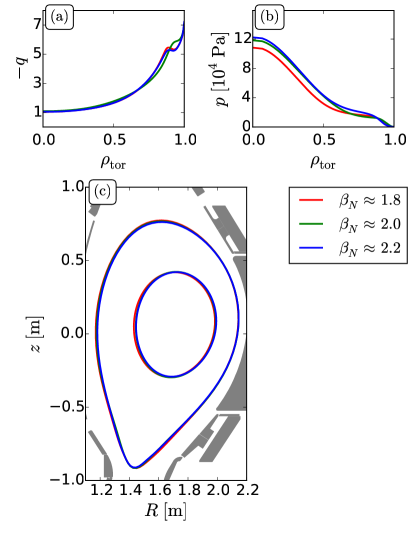
Figure 4: Properties of the three input equilibria. (a) q-profile and (b) pressure profiles versus $\rho\rm{{}_{tor}}$. (c) $\acs{rhotor}=0.5$ and $1.0$ surface for low (red), medium (green) and high $\beta\rm{{}_{N}}$ (blue) case. The corresponding shots are colored in table 1.

To avoid any influence of the rigid rotation and of ELM physics on the equilibrium reconstruction, we use for the initial 2D equilibrium only pre-ELM time-points from the magnetic signals averaged over one rotation period. This is very similar to the procedure used for the synchronization of the ELM cycle [42]. Then, only pre-ELM measurements from interferometry, LIB, ECE, CXRS and Thomson scattering (TS) are used for the edge pressure profile to further constrain the 2D equilibria (figure 4(a)). The $n\rm{{}_{e}}$ and $T\rm{{}_{e}}$ profiles from TS are used to align the profiles. To account for the change in the edge pressure gradient due to the density pump-out, we use input equilibria once with strongest density ’pump-out’ resulting in low $\beta\rm{{}_{N}}$ (red) and once with almost no ’pump-out’ leading to relatively high $\beta\rm{{}_{N}}$ (blue). Since VMEC cannot handle the SOL, we excluded SOL currents in the CLISTE equilibrium reconstruction. Moreover, the edge $q$ profile in CLISTE is constrained to match the Sauter predictions for the bootstrap current [43] using $n\rm{{}_{e}}$ and $T\rm{{}_{e}}$ profile measurements mentioned previously (figure 4(a)). Consequently, the resulting edge $q$ and pressure profiles in the equilibrium have experimental uncertainties depending on the measurements accuracy and on the alignment between the density and the temperature profiles. These uncertainties are taken into account by including one input equilibrium at medium $\beta\rm{{}_{N}}$, which exhibits a more outwardly shifted density profile [44]. This changes the edge pressure profile and the $q$-profile (green in figure 4). In total, we estimated that the uncertainties of the edge $q$-profiles are around $\pm 10\%$. The reason for this outward shift in the density profile is not clear. Since it is also present during the phases without MP-field, we can rule out possible 3D effects as the cause. One possible explanation might be some changes in the divertor condition due to different wall conditions after the boronization, which is difficult to diagnose. However, the inclusion of the various equilibria allows us to estimate the impact of such profile uncertainties in the input equilibria on the 3D distortion of the flux surfaces. Although there are some variations in the equilibrium profiles in all cases, the shape of the LCFS is almost the same (figure 4(c)).

3.3 Displacement calculated using the vacuum field approximation

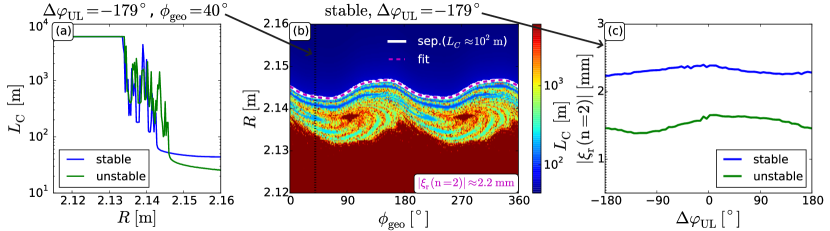
Figure 5: (a) Connection length $L\rm{{}_{C}}$ along the LFS midplane using the stable (blue) and the unstable (green) manifold at a single toroidal position $\phi{\rm{{}_{geo}}}$ and $\Delta\varphi\rm{{}_{UL}}$. (b) Laminar plot of $L\rm{{}_{C}}$ using the stable manifold along the toroidal coordinate $\phi{\rm{{}_{geo}}}$. $L\rm{{}_{C}}$ of $100\ \rm{m}$ to determine an ’effective’ boundary and a displacement amplitude $\xi_{r}$. (c) The boundary displacement using stable and unstable manifold versus $\Delta\varphi\rm{{}_{UL}}$. Amplitudes are not larger than $2.4\ \rm{mm}$.

To underline the importance of the plasma response, measurements of the boundary displacement can be compared with predictions from vacuum field-line tracing. These predictions ignore shielding of the applied MP-field and the amplification by stable ideal kink modes. The determination of a boundary displacement from vacuum field calculations is somewhat critical since a LCFS is not necessarily preserved because of changes in the magnetic topology due to ergodization. However, one can estimate an ’effective’ plasma boundary by a sudden increase of the connection length of the field-lines using equilibrium field superimposed with the applied MP-field. Figure 5(a) shows the calculated Connection length ($L\rm{{}_{C}}$) between the LOS along the LFS midplane and the target at one geometric toroidal coordinate $\phi\rm{{}_{geo}}=40^{\circ}$. Since it is possible to follow the field-line in two directions, we refer to the direction towards the inner target as stable manifold and towards the outer target as unstable manifold (page 187 in Ref. [45]). The applied MP-field in figure 5(a) has $\acs{dphi}=-179^{\circ}$ ($\approx$vacuum resonant). Field-line tracing is stopped when $L\rm{{}_{C}}$ reaches $6\ \rm{km}$. A sudden rise of $L\rm{{}_{C}}$ can be clearly identified at a $L\rm{{}_{C}}$ of around $10^{2}\ \rm{m}$, which is similar to the separatrix value in the axisymmetric case. Hence, we use this threshold ($\acs{LC}\approx 10^{2}\ \rm{m}$) to define an ’effective’ plasma boundary. These calculations are then extended to all toroidal positions, which allows us to determine an ’effective’ $n=2$ boundary displacement. An example using the stable manifold is shown in figure 5(b). The solid white line is the ’effective’ plasma boundary and the magenta dashed line is the sinusoidal fit to it. The derived amplitude is $2.2\ \rm{mm}$. This procedure is applied to all $\Delta\varphi\rm{{}_{UL}}$s in the scan using both, the stable and the unstable manifolds (figure 5(c)). The radial displacements for all cases are smaller than $\pm 2.4\ \rm{mm}$.

A combination of using the stable and the unstable manifolds does not increase the ’effective’ boundary displacement. Instead, it leads to additional harmonic components. Additionally, the implementation of shielding on resonant surfaces would result in even smaller displacements. For simplicity reasons, only the equilibrium with medium $\beta\rm{{}_{N}}$ (green in figure 4) is used for the vacuum field calculations. The choice of the equilibrium has only a small impact on the ’effective’ boundary displacement evaluated using the vacuum field approximation.

3.4 3D ideal MHD equilibrium calculations, VMEC

In the experiments presented here $T\rm{{}_{e}}$ at the pedestal top is above $1\;\rm{keV}$ resulting in a low resistivity. The perpendicular electron velocity is also high and has no zero-crossing in the pedestal (see also Section 4.3 in Ref. [26]). Furthermore, we have no indication of mode penetration due to externally applied MPs like the $T\rm{{}_{e}}$ perturbations being in anti-phase on both sides of a rational surface or a flattening of the profile at a rational surface. These reasons justify to compare the measured displacement with the one from an ideal MHD code.

For the following comparison, we use a free boundary version of the ideal MHD equilibrium code VMEC (also called NEMEC [14]). VMEC is able to calculate the 3D distorted flux surfaces. To parameterize its geometry it uses a Fourier representation. VMEC minimizes the plasma energy ($W\rm{{}_{MHD}}$) by solving the variational problem $dW\rm{{}_{MHD}}/dt=0$ using the steepest-descent moment method [13]. To avoid time-consuming calculations which do not converge [46], we first test if the axisymmetric case (free boundary) converges using a small amount of flux surfaces ($\approx 200$). If necessary, we adapt configuration parameters, such as the amount of poloidal mode numbers, and use the same parameters for the extensive 3D cases [47]. These 3D calculations usually converge without any difficulties. To assure a sufficient resolution for all 3D calculations, we use 1001 flux surfaces, 17 toroidal mode numbers for one period ($\phi\rm{{}_{geo}}=0-180^{\circ}$ for the $n=2$ perturbation) including the negative ones ($n=-16,-14,\dots,14,16$) and 26 poloidal mode numbers. The choice of a sufficiently high resolved grid is essential, otherwise the calculated displacements can be underestimated (see A). For this study, the input equilibria for all calculations are truncated at a normalized poloidal flux of 0.9999 (details about truncation in VMEC in Ref. [47]).

In total, we calculated 27 3D VMEC equilibria using three different input equilibria and nine different $\Delta\varphi\rm{{}_{UL}}$ configurations. The main purpose of the variations in the $q$ and pressure profile of the input equilibria is to estimate their influence on the uncertainties of the displacement.

4 Plasma response as indicated by ELM and density behavior

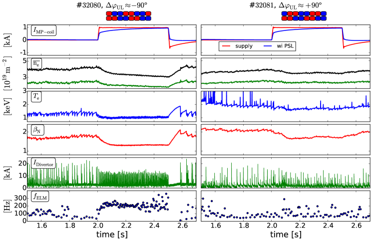
Figure 6: Correlation between plasma response and ELM behavior. Time traces of discharge $\#32080$ using $\Delta\varphi\rm{{}_{UL}}$ of $-90^{\circ}$ (left) and discharge 32081 with $+90^{\circ}$ (right). Insets at the top indicate the coil configurations. From top to bottom: MP-coil supply current (red) and ’effective’ (blue) current of one coil, core and edge chord of line integrated $n\rm{{}_{e}}$, edge $T\rm{{}_{e}}$ from ECE, normalized beta $\beta_{N}$, divertor current and ELM frequency. ELM behavior and $n\rm{{}_{e}}$ are clearly changed for $\acs{dphi}\approx-90^{\circ}$.

Empirically, the calculated displacement around the X-point, the top and the HFS correlate with the ELM frequency and the density ’pump-out’ [2, 3, 4]. Hence, the simplest method to test the plasma response is to vary the applied mode spectrum via $\Delta\varphi\rm{{}_{UL}}$ and observe the change in ELM frequency as well as density. This can be realized either by a continuous scan of $\Delta\varphi\rm{{}_{UL}}$ or by applying several static MP-phases with different $\Delta\varphi\rm{{}_{UL}}$. The first one has been done for a very similar plasma scenario, which only differs by a slight adaption of the upper shape to enable fast ion loss detector measurements [48]. This change is marginal suggesting a marginal impact on the plasma response [49]. The comparison between MARS-F calculations [50] and the axisymmetric plasma response (e.g. $n\rm{{}_{e}}$, ELM frequency) is shown in figure 7 in Ref. [39]. The strongest response in the measurements and calculations are around $\acs{dphi}\approx-90^{\circ}$. The fact that $\acs{dphi}\approx-90^{\circ}$ is clear away from the optimum field alignment $\acs{dphi}\approx\pm 180^{\circ}$ underlines the role of the stable ideal kink modes at poloidal mode numbers larger than the resonant components ($m>nq$).

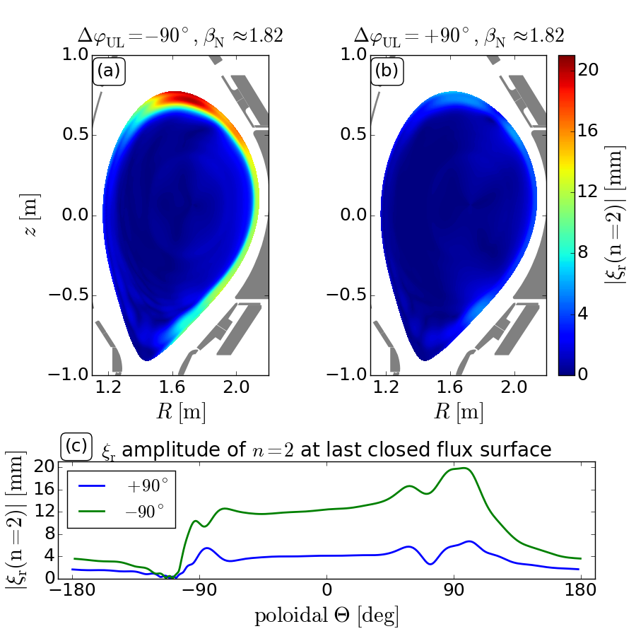
Figure 7: The poloidal distribution of the $n=2$ displacement amplitude applying (a) $\acs{dphi}\approx-90^{\circ}$ and (b) $\acs{dphi}\approx+90^{\circ}$ using the same input equilibrium with the same $\beta\rm{{}_{N}}$. (c) displacement amplitude at the LCFS versus poloidal angle. The $-90^{\circ}$ case has larger displacements.

To verify this behavior for the identical configuration used for the rigid rotations, we conducted experiments applying static MP-fields using $\acs{dphi}\approx-90^{\circ}$ (figure 6 (left)) and $+90^{\circ}$ (right). Clear changes in the confinement and ELM frequency are observed depending on the applied coil configuration. To emphasize the effect of the MP-field on $n_{e}$ and $T_{e}$, the MP-field is switched-off ’fast’ by compensating the image currents in the PSL using counteracting coil currents [3, 51]. This compensation occurs within milliseconds and is illustrated in the top frames of figure 6 showing the applied coil current (red) of one MP-coil and the corresponding effective coil current including the PSL response (blue). During this ’fast’ switch-off of the $-90^{\circ}$ configuration, ELMs disappear simultaneously with the MP-field, which is typical for MHD timescales (see Ref. [3]). Afterwards, $n_{e}$ and $T_{e}$ recovers on transport time scales typical for the pedestal build-up after the transition from L- to H-mode (see e.g. Ref. [33]). For $\acs{dphi}\approx+90^{\circ}$, almost no effect on the ELM and density behavior is seen.

To analyze the role of the displacement, we calculated the corresponding radial displacement using VMEC with the same $\beta\rm{{}_{N}}$ as shown in figure 7. The $n=2$ displacement amplitude, especially around the plasma top, is clearly stronger for the $-90^{\circ}$ (a) case than for $+90^{\circ}$ (b). This emphasizes the effect of the displacement on the ELM stability, particle and energy confinement. Note, the LFS and the HFS responses of this plasma configuration have a very similar dependence on $\Delta\varphi\rm{{}_{UL}}$, which is indicated in figure 7(c) and the following sections. This is a feature of the investigated plasma configuration and does not hold generally as suggested by calculations based on other ASDEX Upgrade configurations [50] and other machines [6]. One should also keep in mind that the displacement in the static experiments are expected to be roughly two times larger than the one in the rigid rotation experiments. This is because the static experiments have full current in each coil (see insets of figure 6), which is not possible in rotation experiments. This increases the field strength by a factor of $\sqrt{2}$. They also have no PSL attenuation, which results in a factor of $1.5$ stronger MP-field.

In summary, the importance of 3D MHD physics on the ELM stability and the particle transport is underlined by the effect of the different applied $\Delta\varphi\rm{{}_{UL}}$s and by the timescales during the ’fast’ switch-off.

5 Plasma top displacement

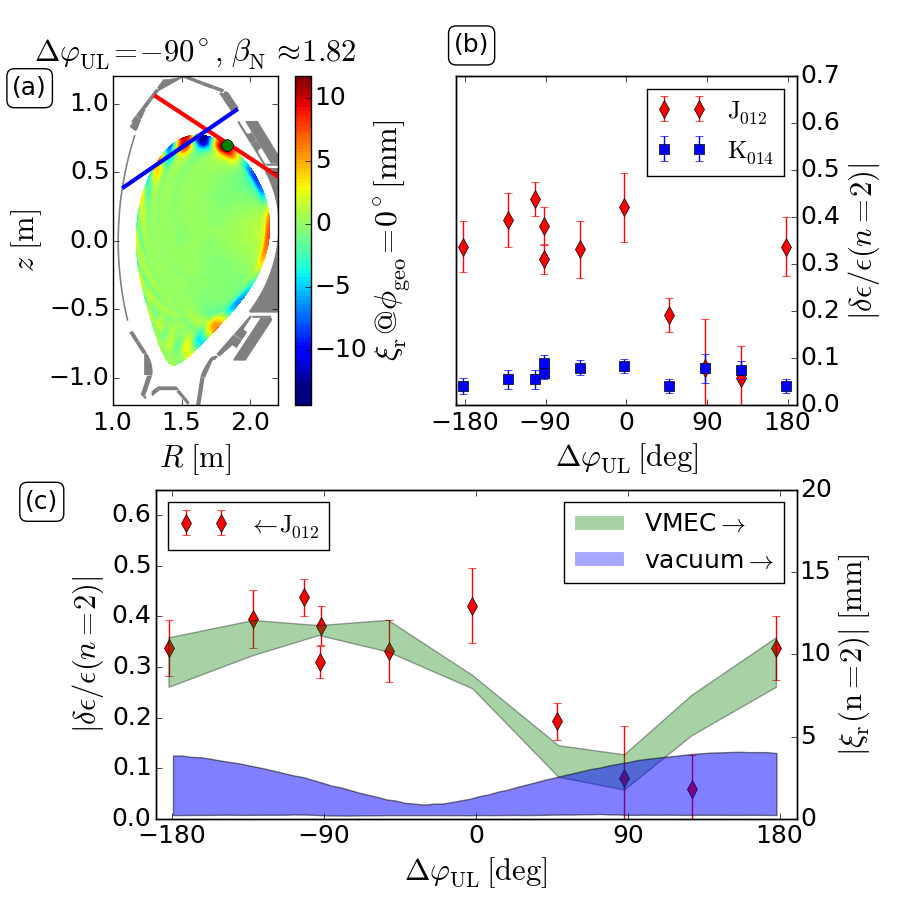
Figure 8: Comparing the displacements at the plasma top. (a) poloidal cut of the displacement $\xi\rm{{}_{r}}$ at one toroidal position $\phi\rm{{}_{geo}}=0^{\circ}$ and LOS of two soft X-ray channels. (b) relative emissivity ($\delta\epsilon/\epsilon$) of $n=2$ versus $\Delta\varphi\rm{{}_{UL}}$ from the two channels in (a). (c) qualitative comparison relative emissivity from one channel with displacement amplitudes from VMEC and vacuum calculations at the position indicated by the green circle in (a). Only a qualitative comparison is possible. Displacements are largest around $\acs{dphi}\approx-90^{\circ}$.

In this section, we further investigate the correlation between the applied poloidal mode spectrum $\Delta\varphi\rm{{}_{UL}}$ and the displacement around the plasma top. We expect the strongest response at the plasma top around $\acs{dphi}\approx-90^{\circ}$ from the behavior of the ELM frequency as well as the density ’pump-out’ mentioned previously in section 4. This is clearly underlined by soft X-ray measurements viewing tangentially to the boundary of the plasma top (geometry in Fig 8(a)).

Figure 8(b) shows the relative emissivity ($\delta\epsilon/\epsilon$) of the $n=2$ perturbation from two soft X-ray channels determined from the various rigid rotation phase versus $\Delta\varphi\rm{{}_{UL}}$. One point corresponds to one rigid rotation phase and one channel. The relative emissivity from the channel $J_{012}$ clearly peaks around $\acs{dphi}\approx-90^{\circ}$. This channel is almost perfectly tangential to the boundary and its relative emissivity is therefore a good indicator for the displacement. To illustrate that channels which are not perfectly tangential to the boundary do not deliver useful displacement data, we add measurements from a second channel $K_{014}$. This channel is not able to resolve the perturbation structures, because it simultaneously views the maximum and minimum displacement as demonstrated by the poloidal cut in figure 8(a). Thus, the perturbation in the emissivity is always small and not a good measure for the displacement.

However, the measurements from channel $J_{012}$ can be used to qualitatively compare them to the amplitude of radial displacement calculated using VMEC and the vacuum field approximation shown in Fig. 8(c). The radial displacement is calculated where the channel LOS crosses the boundary indicated by a green circle in Fig. 8(a). The green shaded area in Fig. 8(c) shows the possible VMEC solutions and the blue shaded are the possible solutions using the vacuum field approximation. For the comparison, only the amplitudes of the dominant toroidal component ($n=2$) are shown. The predicted VMEC and observed displacement amplitudes have their maxima at $\acs{dphi}\approx-90^{\circ}$ as well as minima at around $+90^{\circ}$ and correlate strongly with the ELM behaviour from the previous section. The vacuum field approximation does not reflect the $\Delta\varphi\rm{{}_{UL}}$ dependency at all and predicts clearly lower displacements than VMEC.

6 LFS midplane displacement

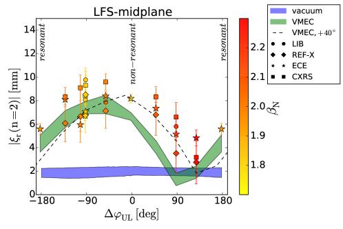
Figure 9: Amplitude of the $n=2$ radial displacements versus $\Delta\varphi\rm{{}_{UL}}$. Each symbol is the measured displacement of one rigid rotation phase determined by one diagnostic. The color scaling indicates the measured $\beta\rm{{}_{N}}$. The possible solutions using the vacuum field approximation and VMEC are indicated by blue and green shaded areas, respectively. The dashed line shows the maxima of the VMEC solutions shifted by $40^{\circ}$. Except for a shift of around $40^{\circ}$, VMEC and the measurements agree well.

In the previous section, the radial displacement between the predictions from VMEC and the measurements were qualitatively compared. In this section, we go a step further and aim to make a quantitative comparison using the high resolution diagnostics around the LFS midplane. To increase the accuracy of the analysis, the effects of the PCS are included (section 2.4). Although the LFS response is thought to play a minor role in the ELM-mitigation [6], this comparison is very valuable to benchmark VMEC.

To merge the various displacement measurements around the LFS midplane using different diagnostics and experiments into one comparison, it is necessary to add the following considerations to the analysis: (i) there is one rigid rotation using $3\ \rm{Hz}$. To compare it to the $2\ \rm{Hz}$ experiments, we simply multiply the evaluated displacement at $3\ \rm{Hz}$ by 1.08 to account for the additional attenuation due to the PSL response. This factor comes from the ratio between the $2\ \rm{Hz}$ and $3\ \rm{Hz}$ attenuation (see section 3.1). (ii) The various LOS of the profile diagnostics are not exactly perpendicular to the axisymmetric surface. Hence, we map the displacement onto the normal using the axisymmetric shape from figure 4, which allows us to compare it with the calculated radial displacement. The largest impact on the displacement amplitude is seen in the case of the LIB geometry, where it changes by only $5\%$. (iii) The diagnostics are not exactly located on the LFS midplane. To account for poloidal asymmetries, we scale the measured displacement to the midplane using the ratio between the calculated displacement at the LOS and the midplane. To get this ratio, we use the average of the three VMEC calculations at the corresponding $\Delta\varphi\rm{{}_{UL}}$. Again, the evaluations of the LIB measurements are primarily affected and the ’worst’ case requires a change of only $18\%$, which is less than $1\ \rm{mm}$.

Figure 9 shows the radial displacement amplitudes ($n=2$) around the LFS midplane versus $\Delta\varphi\rm{{}_{UL}}$ from the measurements, from the VMEC solutions (green shaded area) as well as from the vacuum field calculations (blue shaded areas). Good agreement can be found between the measurements and the VMEC calculations. When the stable ideal kink modes are expected to be excited, both clearly surpass the prediction from the vacuum field calculations, no matter which manifold is used. It is also seen from the range of the green shaded area that the observed variation in $\beta\rm{{}_{N}}$, in the edge pressure gradient and in the $q$-profile have no large impact on the calculated displacement amplitude from VMEC. Additionally, a slightly different choice of the used resolution in VMEC can increase the calculated displacement amplitude by $1\;\rm{mm}$ (see A). Then, the agreement with the measurements would be even better. We also observe no systematic difference in the displacement between density and temperature measurements, which underlines the presence of perturbed flux surfaces.

An offset of $40^{\circ}$ in $\Delta\varphi\rm{{}_{UL}}$ between the measurements and the VMEC calculations indicates a minor disagreement. This offset is outside the measurement uncertainties of the displacement amplitude and outside the possible range of VMEC calculations. The applied poloidal mode spectra and thus, the $\Delta\varphi\rm{{}_{UL}}$ dependence of the plasma response depends strongly on the positions of the flux surfaces due to the Grad-Shafranov shift, thus, $\beta\rm{{}_{N}}$ and on the $q$-profile. The considered variations in the $q$-profile (figure 4) alone shifts the $\Delta\varphi\rm{{}_{UL}}$ dependence of the resonant components from vacuum field calculations by $30^{\circ}$. But as seen in figure 9, the LFS response is only shifted by $10^{\circ}$. Thus, the considered variations in the $q$- and pressure profile are not enough to explain these discrepancies in $\Delta\varphi\rm{{}_{UL}}$ in the case of the LFS response. It should be noted that the $q$- and pressure profile have not been varied independently.

7 Summary and Discussion

The main goal of this paper was to quantitatively compare measurements of the boundary displacement to ideal MHD modeling using VMEC. Rigidly rotating $n=2$ MP-fields with different $\Delta\varphi\rm{{}_{UL}}$ and toroidally localized diagnostics deliver the accuracy which is needed to measure the displacement and its dependence on the applied poloidal mode spectrum. To keep the margins for interpretation from the experimental side small, we included various profile diagnostics in the analysis. Furthermore, we accounted for additional plasma movements due to the plasma control system and varied the applied poloidal mode spectrum using $\Delta\varphi\rm{{}_{UL}}$. For both the experimental analysis and the modeling input, only pre-ELM data were used. On the modeling side, we consider the MP-field attenuation due to passive conductors (PSL), the changes in the edge pressure profile due to the density ’pump-out’ and the small variations in the $q$-profile. To avoid any misinterpretation due to ’inadequate’ grid settings, we also performed sensitivity studies on the grid resolution (see A).

From this comprehensive study, we conclude that VMEC correctly predicts the boundary displacement amplitude due to stable ideal kink modes excited by external MP-fields. Good quantitative agreement around the LFS midplane is found. The HFS response around the plasma top could only be compared qualitatively mainly due to the lack of locally available diagnostics. Although VMEC cannot resolve localized sheet currents, assumes nested flux surface and hence, has no resistive MHD, no SOL physics and no toroidal rotation included [29], it reproduces the amplitude of the displacement and its dependences on $\Delta\varphi\rm{{}_{UL}}$. The only caveat is that there is a systematic offset of around $40^{\circ}$ in $\Delta\varphi\rm{{}_{UL}}$ between the measurements and the modeling around the LFS midplane. This motivates further studies on the impact of the $q$-profile on the $\Delta\varphi\rm{{}_{UL}}$ behavior. To rule out a lack of physics like SOL currents, two-fluid MHD [12], toroidal rotation [29] or localized sheet currents [52] as a possible explanation for the shift in $\Delta\varphi\rm{{}_{UL}}$, further comparisons to other MHD codes [8, 53] like IPEC, JOREK, MARS-F and M3D-C1 are needed.

In conclusion, we can state that, if no strong resistive MHD mode activity like mode penetration is present, VMEC can properly compute the 3D perturbation of the flux surface at the boundary.

8 Acknowledgement

M.W. would like to thank J. Loizu for fruitful discussions. This work has been carried out within the framework of the EUROfusion Consortium and has received funding from the Euratom research and training programme 2014-2018 under grant agreement No 633053. The views and opinions expressed herein do not necessarily reflect those of the European Commission.

Appendix A Grid resolution of VMEC

The grid resolution in VMEC is often discussed [54, 47, 55] and is crucial for a reliable prediction from VMEC. To avoid any misinterpretation because of a too low grid resolution, we scanned the number of flux surface, of poloidal and of toroidal mode numbers. The default setting for this study is 1001 flux surfaces, 17 toroidal mode numbers and 26 poloidal mode numbers for one $n=2$ period ($\phi\rm{{}_{geo}}=0-180^{\circ}$).

A.1 Number of flux surfaces

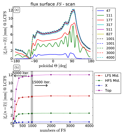
Figure 10: Sensitivity study on the numbers of flux surfaces (FS). (a) The $n=2$ displacement amplitude at the LCFS versus poloidal angle $\Theta$. (b) Displacement versus numbers of FS for specific poloidal positions. The grey bar indicates the default resolution.

To study the impact of the radial resolution on the resulting displacement [55], we increased the amount of flux surfaces up to 4000. We pick a case with a strong plasma response ($\acs{dphi}\approx-90^{\circ}$, low $\beta\rm{{}_{N}}$ and $2\;\rm{Hz}$). Figure 10 shows the sensitivity study on the number of flux surfaces. The displacement at the LCFS versus the poloidal angle is shown in figure 10(a). Figure 10(b) illustrates the displacement at the LFS midplane ($\Theta=0^{\circ}$), plasma top ($+90^{\circ}$), LFS midplane ($\pm 180^{\circ}$) and the X-point. One should note that for less than 1000 flux surfaces, 5000 iterations are used, whereas for more than 1000 surfaces 15000 iterations are used. However even with 4000 flux surfaces, the maximum displacement does not change more than $0.2\;\rm{mm}$ with respect to the used number of 1001. This is not a surprise, since (i) VMEC uses an equidistant toroidal flux grid (in this version), which is relatively dense towards the edge and (ii) we are studying an experimental configuration which primarily exhibits edge perturbations.

A.2 Number of poloidal mode numbers

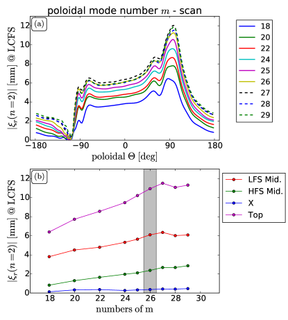
Figure 11: Sensitivity study on the numbers of poloidal mode numbers $m$. (a) The $n=2$ displacement amplitude at the LCFS versus poloidal angle $\Theta$. (b) Displacement versus numbers of $m$ for specific poloidal positions. The grey bar indicates the default resolution.

In this and the following comparison, we use the $3\;\rm{Hz}$ MP-field attenuation . A minimum of 18 poloidal mode numbers is required to reproduce the axisymmetric elongated shape. This number is still far too low to get reasonable displacement values, because they increase until they stagnate around 26 (Figure 11(b)).

A.3 Number of toroidal mode numbers

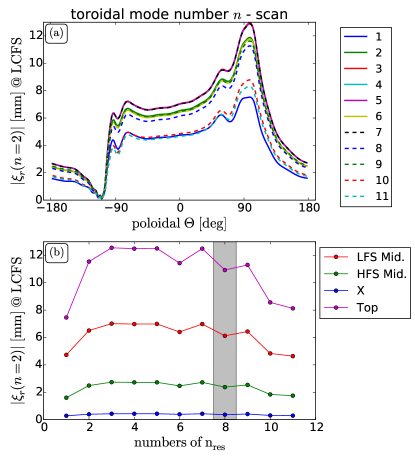
Figure 12: Sensitivity study on the numbers of toroidal mode numbers $n{{}_{res}}$ using one period ($\phi\rm{{}_{geo}}=0-180^{\circ}$). (a) The $n=2$ displacement amplitude at the LCFS versus poloidal angle $\Theta$. (b) Displacement versus numbers of $n{{}_{res}}$ for specific poloidal positions. The grey bar indicates the default resolution. $n{{}_{res}}=8$ means that we consider up to $n=16$.

The input parameter in VMEC for the toroidal resolution $n{{}_{res}}$ also accounts for the negative mode number. Employing $n{{}_{res}}=8$ for one $n=2$ period ($\phi\rm{{}_{geo}}=0-180^{\circ}$) means 17 toroidal mode numbers. The numbers of toroidal angles ($\zeta$) are used to describe the vacuum field perturbations from the MP-coils for the boundary condition. Usually, we set $\zeta$ four time larger than $n{{}_{res}}$. During this sensitivity study, it turned out that, at least, $\acs{zeta}=32$ are required to describe the $n=2$ vacuum field perturbations for one period (4 coils in each row). Otherwise the VMEC calculations did not converge. So for $n{{}_{res}}<9$, we used a $\zeta$ of 32 and otherwise, four times of $n{{}_{res}}$. Figure 12 shows the sensitivity study. Already $n{{}_{res}}=3$ delivers reasonable results. But using $n{{}_{res}}=3$ instead of $n{{}_{res}}=8$ does not save a lot of computational time, since the vacuum calculations with $\acs{zeta}=32$ are the most time consuming part. However, for larger toroidal mode numbers $n{{}_{res}}>8$ the amplitude of the dominant mode decreases. A similar behavior is given, when too many harmonics of a sine fine are given to fit experimental data. Then, the amplitude of $n=2$ decreases with increasing harmonics as well. We assume that this is also the case when the amount of toroidal mode numbers in VMEC increases.

References

- [1] T. E. Evans et al. Physical Review Letters, 92:235003, 2004.
- [2] A. Kirk et al. Nuclear Fusion, 55(4):043011, 2015.
- [3] W. Suttrop et al. Plasma Physics and Controlled Fusion, 59(1):014049, 2017.
- [4] C. Paz-Soldan et al. Physical Review Letters, 114:105001, 2015.
- [5] Y. Q. Liu et al. Nuclear Fusion, 51(8):083002, 2011.
- [6] C. Paz-Soldan et al. Nuclear Fusion, 56(5):056001, 2016.
- [7] R. A. Moyer et al. Nuclear Fusion, 52(12):123019, 2012.
- [8] J. D. King et al. Physics of Plasma, 22(11), 2015.
- [9] J. K. Park et al. Physics of Plasma, 14(5):052110, 2007.
- [10] F. Orain et al. Nuclear Fusion, 57(2):022013, 2017.
- [11] Y. Q. Liu et al. Physics of Plasma, 7(9):3681, 2000.
- [12] N. M. Ferraro et al. Nuclear Fusion, 53(7):073042, 2013.
- [13] S. P. Hirshman et al. Physics of Fluids, 26(12):3553, 1983.
- [14] E. Strumberger et al. Nuclear Fusion, 54(6):064019, 2014.
- [15] I. T. Chapman et al. Physics of Plasmas, 20(5), 2013.
- [16] T.M. Bird et al. Nuclear Fusion, 53(1):013004, 2013.
- [17] V. Bobkov et al. AIP Conference Proceedings, 1580(1):271–274, 2014.
- [18] R. Fischer et al. Plasma Physics and Controlled Fusion, 54(11):115008, 2012.
- [19] J. C. Fuchs et al. Investigation of the boundary distortions in the presence of rotating external magnetic perturbations on ASDEX Upgrade. 41th EPS Conference on Plasma Phys., 2014.
- [20] M J Lanctot et al. Physics of Plasma, 18(5):056121, 2011.
- [21] I. T. Chapman et al. Plasma Physics and Controlled Fusion, 54(10):105013, 2012.
- [22] I. T. Chapman et al. Nuclear Fusion, 47(11):L36, 2007.
- [23] D. Yadykin et al. Plasma Physics and Controlled Fusion, 57(10):104003, 2015.
- [24] I. T. Chapman et al. Nuclear Fusion, 54(8):083006, 2014.
- [25] D. Orlov et al. Nuclear Fusion, 54(9):093008, 2014.
- [26] M. Willensdorfer et al. Plasma Physics and Controlled Fusion, 58(11):114004, 2016.
- [27] W. Suttrop et al. Plasma Physics and Controlled Fusion, 53(12):124014, 2011.
- [28] S. A. Lazerson and the DIII-D Team. Nuclear Fusion, 55(2):023009, 2015.
- [29] A. Wingen et al. Nuclear Fusion, 57(1):016013, 2017.
- [30] J J Koliner et al. Physics of Plasma, 23(3):032508, 2016.
- [31] S. K. Rathgeber et al. Plasma Physics and Controlled Fusion, 55(2):025004, 2013.
- [32] M. Willensdorfer et al. Review of Scientific Instruments, 83(2):023501, 2012.
- [33] M. Willensdorfer et al. Plasma Physics and Controlled Fusion, 56(2):025008–10, 2014.
- [34] E. Viezzer et al. Review of Scientific Instruments, 83(10):103501, 2012.
- [35] A. Medvedeva et al. Density profile and turbulence evolution during L-H transition studied with the Ultra-fast swept reflectometer on ASDEX Upgrade. 43rd EPS Conference on Plasma Phys., 2016.
- [36] I. T. Chapman et al. Plasma Physics and Controlled Fusion, 56(7):075004, 2014.
- [37] R. Fischer et al. Fusion science and technology, 69(2), 2016.
- [38] M. W. Shafer et al. Physics of Plasmas, 21(12):122518, 2014.
- [39] Y. Liu et al. Plasma Physics and Controlled Fusion, 58(11):114005, 2016.
- [40] A. Gude V. Igochine and M. Maraschek. Hotlink based soft x-ray diagnostic on ASDEX Upgrade Report. IPP Report, page 1/338, 2010.
- [41] W. Suttrop. Finite elements calculations from the saddle coils and the PSL. private communication, 2016.
- [42] M. G. Dunne et al. Nuclear Fusion, 52(12):123014, 2012.
- [43] O. Sauter et al. Physics of Plasma, 6(7):2834–2839, 1999.
- [44] M. G. Dunne et al. Plasma Physics and Controlled Fusion, 59(1):014017, 2017.
- [45] Sadrilla Abdullaev. Magnetic Stochasticity in Magnetically Confined Fusion Plasmas. Springer-Verlag, 2014.
- [46] A.D. Turnbull et al. Physics of Plasma, 20(5):056114, 2013.
- [47] A. Wingen et al. Plasma Physics and Controlled Fusion, 57(10):104006, 2015.
- [48] M. Garcia-Munoz et al. Plasma Physics and Controlled Fusion, 55(12):124014, 2013.
- [49] L. Li et al. Nuclear Fusion, 56(12):126007, 2016.
- [50] Y. Liu et al. Nuclear Fusion, 56(5):056015, 2016.
- [51] N. Leuthold et al. Plasma Physics and Controlled Fusion, 59(5):055004, 2017.
- [52] J. Loizu. et al. Physics of Plasma, 23(5), 2016.
- [53] A. Reiman et al. Nuclear Fusion, 55(6):063026, 2015.
- [54] A. D. Turnbull et al. Nuclear Fusion, 52(5):054016, 2012.
- [55] S. A. Lazerson et al. Physics of Plasma, 23(1):012507, 2016.