Methods for analysis of two-particle rapidity correlation function in high-energy heavy-ion collisions

Abstract

Two-particle rapidity (or pseudorapidity) correlation function $C(y_{1},y_{2})$ was used in analysing fluctuation of particle density distribution in rapidity in high-energy heavy-ion collisions. In our research, we argue that for a centrality window, some additional correlation may be caused by a centrality span, when the mean two- and single-particle densities over a centrality window are used directly in the calculation , just like $\left<N(y_{1},y_{2})\right>/\left[\left<N(y_{1})\right>\left<N(y_{2})\right>\right]$. We concentrate on removing the influence of collision-centrality span on correlation function, and two calculation methods are raised. In one method, correlation coefficients are considered to be the ratios of probabilities (not the particle density). In the other method, a relative multiplicity is introduced to unity the events of different centralities. For testing the methods, ampt model is used and a toy granular model is built to simulate the fluctuation of particle density in rapidity.

I Introduction

Hot and dense matter is created in high-energy heavy-ion collisions. The fluctuation of stopping at early stage may lead an event-by-event fluctuation of particle density in rapidity at final stage Bzdak and Teaney (2013); Jia et al. (2016a, b); Bozek et al. (2011); Jia and Huo (2014); Bhalerao et al. (2015); Pang et al. (2015); Khachatryan et al. (2015). The particle density fluctuation in rapidity can be fully parameterized with a group of polynomials Bzdak and Teaney (2013), such as Chebyshev polynomials Bzdak and Teaney (2013), Legendre polynomials Jia et al. (2016a) or some other orthogonal polynomials, just like

$$\rho\left(y;a_{1},a_{2},\cdots\right)=\rho_{0}\left(y\right)\Big{[}1+\sum_{n=0}^{\infty}a_{n}T_{n}\left(y\right)\Big{]},$$ (1)

where $\rho(y;a_{1},a_{2},\cdots)$ is the single particle density of an event, $\rho_{0}(y)$ is the mean particle density over the events. In Ref. Jia et al. (2016a), $T_{n}(y)\equiv\sqrt{n+\frac{1}{2}}P_{n}(y/Y)$, where the $P_{0}(x)=1$, $P_{1}(x)=x$, $P_{2}(x)=(3x^{2}-1)/2$, $\cdots$ are Legendre polynomials and illustrated in Fig. 1, and $Y$ characterizes the range of rapidity fluctuation, $\left|y\right|<Y$ (Here, $Y=6$). The event-by-event fluctuation of the rapidity distribution is described by the parameters $a_{n}$. For instance, $a_{1}$ reflects the asymmetry Bialas and Zalewski (2010) of particle density distribution in rapidity of an event. $\left<a_{1}\right>$ is null in the symmetrical collision system, and $\left<a_{1}^{2}\right>$ does not have to be null. The variance reflects how the longitudinal shape is changing event by event. On the other hand, purely statistical particle multiplicity fluctuation can also cause event-by-event fluctuation in rapidity. Therefore, $\left<a^{2}_{n}\right>=\left<(a_{n}^{\textmd{obs}})^{2}\right>-\left<(a_{n}^{\textmd{ran}})^{2}\right>$ was used for describing pure event-by-event shape fluctuation (nonstatistical component of these longitudinal harmonics) Jia et al. (2016a), where $a_{n}^{\textmd{obs}}$ characterizes the fluctuations due to finite number of particles in the events, and $a_{n}^{\textmd{ran}}$ corresponds purely statistical fluctuation, see Ref. Jia et al. (2016a) or Appendix A.

Two-particle rapidity correlation function $C(y_{1},y_{2})$ was used for calculating $\left<a_{n}^{2}\right>$ Bzdak and Teaney (2013); Radhakrishnan (2016). The definition of two-particle rapidity correlation function (2PC) can be obtained by comparing the double charged hadrons inclusive cross section $d^{2}\sigma_{2\textmd{ch}}/dy_{1}dy_{2}$ to the product of single charged particle inclusive cross sections $d\sigma_{1\textmd{ch}}/dy$. The definition of correlation function $C(y_{1},y_{2})$ can be expressed as

$$C(y_{1},y_{2})=\frac{\left<n_{\textmd{ch}}\right>^{2}}{\left<n_{\textmd{ch}}(n_{\textmd{ch}}-1)\right>}\cdot\frac{\sigma_{\textmd{ch}}d^{2}\sigma_{\textmd{2ch}}/dy_{1}dy_{2}}{\left(d\sigma_{\textmd{1ch}}/dy_{1}\right)\left(d\sigma_{\textmd{1ch}}/dy_{2}\right)}$$ (2)

where $\sigma_{\textmd{ch}}$ is the total charged hadron production cross section, and $n_{\textmd{ch}}$ is the charged hadron multiplicity. The ratio of multiplicity moments is caused by the normalization of single- and double-charged hadron inclusive cross sections as

$$\int dy_{1}dy_{2}\left(d^{2}\sigma_{\textmd{2ch}}/dy_{1}dy_{2}\right) = \left<n_{\textmd{ch}}\left(n_{\textmd{ch}}-1\right)\right>\sigma_{\textmd{ch}},$$ (3)

$$\int dy\left(d\sigma_{\textmd{1ch}}/dy\right) = \left<n_{\textmd{ch}}\right>\sigma_{\textmd{ch}}.$$ (4)

This definition Eq. (2) insures that $C\left(y_{1},y_{2}\right)\equiv 1$ when the charged hadrons are uncorrelated Gyulassy et al. (1979).

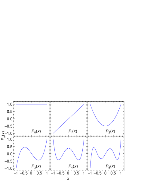
Figure 1: Illustration of Legendre polynomials.

In recent years, two-particle correlation function was usually written as

$$C\left(y_{1},y_{2}\right)=\frac{\rho_{2}\left(y_{1},y_{2}\right)}{\rho_{1}\left(y_{1}\right)\rho_{1}\left(y_{2}\right)},$$ (5)

where $\rho_{2}(y_{1},y_{2})$ and $\rho_{1}(y)$ are two- and single-particle density distribution, respectively Ravan et al. (2014); Vechernin (2015); Monnai and Schenke (2016); Pruneau et al. (2002); Khachatryan et al. (2010); Vechernin (2013). (The differences between Eqs. (2) and (5) are discussed in Sec. II and Appendix C.) At a given $a_{0}$, $a_{1}$, $\cdots$

$$\rho_{2}(y_{1},y_{2};a_{0},a_{1},\cdots)\!=\!\rho_{1}(y_{1};a_{0},a_{1},\cdots)\rho_{1}(y_{2};a_{0},a_{1},\cdots).$$ (6)

Because $\rho_{2}(y_{1},y_{2})$ and $\rho_{1}(y)$ are averages over $a_{i}$, 2PC could be expressed as Bzdak and Teaney (2013); Jia et al. (2016a)

$$C(y_{1},y_{2})\!=\!1\!+\!\!\!\sum_{m,n=0}^{\infty}\!\!\!\left<a_{m}a_{n}\right>\frac{T_{m}(y_{1})T_{n}(y_{2})+T_{m}(y_{2})T_{n}(y_{1})}{2},$$ (7)

and $\left<a_{m}a_{n}\right>$ was expressed as Bzdak and Teaney (2013); Jia et al. (2016a)

$$\left<a_{m}a_{n}\right>= \frac{1}{Y^{2}}\int\left[C\left(y_{1},y_{2}\right)-1\right]$$ (8)

$$\times\frac{T_{m}(y_{1})T_{n}(y_{2})+T_{m}(y_{2})T_{n}(y_{1})}{2}~{}dy_{1}dy_{2},$$

see Ref. Bzdak and Teaney (2013); Jia et al. (2016a) or Appendix B.

But for a centrality window (which is not narrow enough), if the averages $\rho_{2}(y_{1},y_{2})$, $\rho_{1}(y_{1})$, and $\rho_{1}(y_{2})$ are calculated over the events of different centralities, we found that some positive additional correlations may be caused (discussed in detail in Sec. II and Appendix C). For solving such a problem in the calculation of $C(y_{1},y_{2})$ for a centrality window, in Ref. Jia et al. (2016a), events were divided into narrow centrality intervals according to their total multiplicity. And then 2PCs were calculated in each event class. At last, an average of the 2PCs of the centrality intervals was made as the final result of the whole window. By the way, this method is denoted by C${}_{\textmd{average}}$ for being distinguished with other methods in this paper.

In this paper, we try to calculate $C(y_{1},y_{2})$ of a centrality window from other ways to remove or reduce the influence of the centrality window span (or the influence of the mixing of events of different centralities), and a multi-phase transport (ampt) model Lin et al. (2005) at $\sqrt{s_{NN}}=200~{}\mathrm{GeV}$ of Au+Au collisions is utilized. For testing the methods, we made a toy granular model to simulate the event-by-event fluctuation of particle density in rapidity.

This paper is organized as follows. We discuss the additional positive correlations calculated with Eq. (5) in Sec. II. Sec. III shows the methods used for removing or reducing the influence of centrality span. In Sec. IV, the calculation methods are tested with ampt model and a toy granular model. A summary is given in Sec. V.

II additional positive correlation

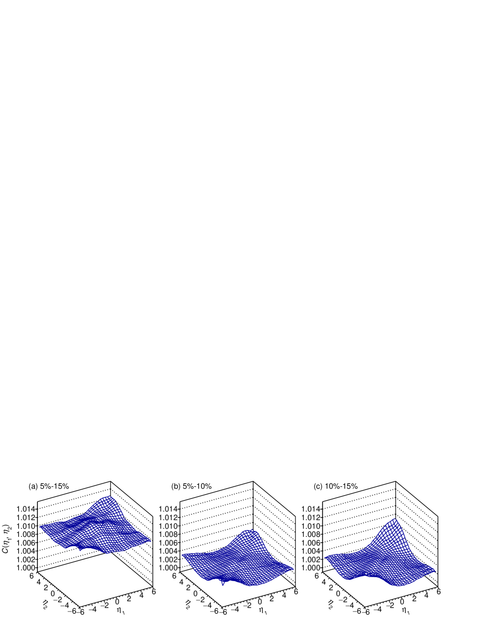
Figure 2: Two-particle pseudorapidity correlation function $C(\eta_{1},\eta_{2})$ of the string melting version ampt model of Au+Au collisions at $\sqrt{s_{NN}}=200~{}\mathrm{GeV}$ (partonic scattering section is $3~{}\mathrm{mb}$), and the results of centrality windows 5%-15%, 5%-10%, and 10%-15% are shown in subgraphs (a), (b), and (c), respectively.

We argue that the mixing of events of different centralities may cause some additional positive correlations, and the reasons are shown as follows.

It is said in section I that $\rho_{1}(y)$ and $\rho_{2}(y_{1},y_{2})$ are mean single particle density in rapidity and mean double particle density over events, respectively. If the events are divided into event classes according to the centrality , single- and double-particle densities in rapidity can be expressed as the averages over the event classes, just like

$$\rho_{1}(y) =\left<\rho_{1}(y;\varepsilon)\right>,$$ (9)

$$\rho_{2}(y_{1},y_{2}) =\left<\rho_{2}(y_{1},y_{2};\varepsilon)\right>,$$

where $\rho_{1}(y;\varepsilon)$ and $\rho_{2}(y_{1},y_{2};\varepsilon)$ stand for the mean single- and double-particle densities of an event class around centrality $\varepsilon$. For explaining where the possible additional positive correlation come from, we assume that $C(y_{1},y_{2};\varepsilon)$ of the event classes are equal to each other (Here, a centrality window divided into $n$ event classes), and $\rho_{1}(y;\varepsilon)$ decreases with increasing centrality $\varepsilon$. Under these assumptions, 2PC of the whole centrality window is bigger than 2PCs of event classes, just like

$$C\left(y_{1},y_{2}\right)>\left<C\left(y_{1},y_{2};\varepsilon\right)\right>=C\left(y_{1},y_{2};\varepsilon\right),$$ (10)

because of

$$\frac{\left<\rho_{2}(y_{1},y_{2};\varepsilon)\right>}{\left<\rho_{1}(y_{1};\varepsilon)\right>\left<\rho_{1}(y_{2};\varepsilon)\right>}>\frac{\left<\rho_{2}(y_{1},y_{2};\varepsilon)\right>}{\left<\rho_{1}(y_{1};\varepsilon)\rho_{1}(y_{2};\varepsilon)\right>}.$$ (11)

Inequality (11) is discussed in detail in Appendix C. We argue that the ”additional correlation” is caused by averaging single- and double-particle densities over a centrality window which is not narrow enough.

For describing such a phenomenon, two-particle pseudorapidity correlation function of the string melting ampt model (partonic scattering section is $3~{}\mathrm{mb}$) of Au+Au collisions at $\sqrt{s_{NN}}=200~{}\mathrm{GeV}$ is utilized. As shown in Fig. 2, the centrality window 5%-15% is divided into two sub-windows 5%-10% and 10%-15%, and 2PC of 5%-15% (Fig. 2a) is higher obviously than 2PCs of 5%-10% (Fig. 2b) and 10%-15% (Fig. 2c). We guess that if the influence of centrality window span on $C(\eta_{1},\eta_{2})$ is removed, 2PC of 5%-15% should be in the middle of 2PCs of 5%-10% and 10%-15% (discussed in Sec. IV).

It is worth to note that in the calculation of 2PC in Fig. 2, $\rho_{1}(\eta)$ is calculated as the ratio of charged particles number $N(\eta)$ in a pseudorapidity interval around $\eta$ to the interval width $\delta\eta$ (in this paper, $\delta\eta=0.1$), just like $\left<N(\eta)\right>/\delta\eta$. And similarly, $\rho_{2}(\eta_{1},\eta_{2})$ is calculated with $\left<N(\eta_{1})N(\eta_{2})\right>/{\delta\eta}^{2}$. Therefore, $C(\eta_{1},\eta_{2})$ can be calculated with the equation $\frac{\left<N(\eta_{1})N(\eta_{2})\right>}{\left<N(\eta_{1})\right>\left<N(\eta_{2})\right>}$. Considering the situation $\eta_{1}=\eta_{2}$, the expression was written as $\frac{\left<N(\eta_{1})N(\eta_{2})\right>}{\left<N(\eta_{1})\right>\left<N(\eta_{2})\right>}-\frac{\delta(\eta_{1}-\eta_{2})}{\left<N(\eta_{1})\right>}$ in Ref. Jia et al. (2016a). On the other hand, for explaining the additional positive correlations, we make an extreme example as follows. We assume that there is no correlation between particles. In other words, particles emit independently and randomly. For a certain centrality $\varepsilon$ (not a centrality window), $C(y_{1},y_{2};\varepsilon)=\frac{\rho_{2}(y_{1},y_{2};\varepsilon)}{\rho_{1}(y_{1};\varepsilon)\rho_{1}(y_{2};\varepsilon)}=1$, which is equivalent to $\rho_{2}(y_{1},y_{2};\varepsilon)=\rho_{1}(y_{1};\varepsilon)\rho_{1}(y_{2};\varepsilon)$. For a centrality window, we assume that $\rho_{1}(y_{1};\varepsilon)$ and $\rho_{1}(y_{2};\varepsilon)$ both decrease with increasing $\varepsilon$, so for the centrality window,

$$\rho_{2}(y_{1},y_{2}) =\left<\rho_{2}(y_{1},y_{2};\varepsilon)\right>$$ (12)

$$=\left<\rho_{1}(y_{1};\varepsilon)\rho_{1}(y_{2};\varepsilon)\right>$$

$$>\left<\rho_{1}(y_{1};\varepsilon)\right>\left<\rho_{1}(y_{2};\varepsilon)\right>$$

$$=\rho_{1}(y_{1})\rho_{1}(y_{2}),$$

which is equivalent to $C(y_{1},y_{2})$ bigger than 1. The detailed discussion is shown in Appendix C.

Where is the additional positive correlation come from? In the normalized definition of two-particle rapidity correlation function Eq. (2), it is obvious when the charged hadrons are uncorrelated, $C(y_{1},y_{2})\equiv 1$. We guess that the additional positive correlation is caused by the 2PC expression Eq. (5) where the particle density distributions are utilized. Single- and double-particle density distributions in rapidity can be expressed as

$$\rho_{1}(y_{1})=d\sigma_{\textmd{1ch}}/\left(\sigma_{\textmd{ch}}dy_{1}\right),~{}~{}\rho_{1}(y_{2})=d\sigma_{\textmd{1ch}}/\left(\sigma_{\textmd{ch}}dy_{2}\right),$$

$$\rho_{2}(y_{1},y_{2})=d^{2}\sigma_{\textmd{2ch}}/\left(\sigma_{\textmd{ch}}dy_{1}dy_{2}\right),$$ (13)

Therefore, the difference between Eqs. (2) and (5) is a ratio $\left<n_{\textmd{ch}}\right>^{2}/\left<n_{\textmd{ch}}\left(n_{\textmd{ch}}-1\right)\right>$. It’s notable that for a specific centrality (or a centrality window narrow enough), if we assume that $n_{\textmd{ch}}$ obeys a Poisson distribution (the variance of $n_{\textmd{ch}}$ is equal to its expectation), $\left<n_{\textmd{ch}}\right>^{2}/\left<n_{\textmd{ch}}\left(n_{\textmd{ch}}-1\right)\right>=1$. But when the centrality window is not narrow enough, the assumption of the Poisson distribution may be not suitable , and some positive correlation may be added.

III methods

For removing or reducing the influence of the mixing of events of different centralities, in Ref. Jia et al. (2016a), events in a centrality window were divided into some narrow centrality intervals. In this section, we try to solve this problem from other ways.

III.1 C${}_{\textmd{defintion}}$ method

In this method, we deduce the expression of $C(y_{1},y_{2})$ (which can be used directly in calculation) from its definition. Eq. (2) can be written in another way as

$$C(y_{1},y_{2})\! = \!\left.\frac{d^{2}\sigma_{\textmd{2ch}}/dy_{1}dy_{2}}{\sigma_{\textmd{ch}}\left<n_{\textmd{ch}}(n_{\textmd{ch}}\!-\!1)\right>}\middle/\left(\!\frac{d\sigma_{\textmd{1ch}}/dy_{1}}{\sigma_{\textmd{ch}}\left<n_{\textmd{ch}}\right>}\!\cdot\!\frac{d\sigma_{\textmd{1ch}}/dy_{2}}{\sigma_{\textmd{ch}}\left<n_{\textmd{ch}}\right>}\!\right)\right.$$ (14)

$$= \left.P_{\textmd{same}}\left(y_{1},y_{2}\right)~{}\middle/~{}\left[P_{1}\left(y_{1}\right)P_{1}\left(y_{2}\right)\right]\right.$$

$$= \left.P_{\textmd{same}}\left(y_{1},y_{2}\right)~{}\middle/~{}P_{\textmd{diff}}\left(y_{1},y_{2}\right)\right.,$$

where $P_{\textmd{same}}(y_{1},y_{2})$ is the probability density of a pair of particles with rapidities $y_{1}$ and $y_{2}$ chosen from the same event, $P_{\textmd{diff}}(y_{1},y_{2})$ is the probability of a pair of particles chosen from different events, which is equal to the product of the single particle probability densities $P(y_{1})$ and $P(y_{2})$. $P_{\textmd{same}}$ and $P_{\textmd{diff}}$ can be expressed as

$$P_{\textmd{same}}\left(y_{1},y_{2}\right)\!\! = \!\!\frac{\sum_{i}\!N_{i}\left(y_{1}\right)N_{i}\left(y_{2}\right)\!-\!\delta(y_{1}\!-\!y_{2})N_{i}\left(y_{1}\right)}{\delta y_{1}\delta y_{2}\sum_{i}n_{{\textmd{ch}},i}\left(n_{{\textmd{ch}},i}-1\right)},~{}~{}~{}~{}~{}~{}$$ (15)

$$P_{\textmd{diff}}\left(y_{1},y_{2}\right) = \frac{\sum_{i\neq j}N_{i}\left(y_{1}\right)N_{j}\left(y_{2}\right)}{\delta y_{1}\delta y_{2}\sum_{i\neq j}n_{\textmd{ch},i}n_{\textmd{ch},j}},$$ (16)

where $i$ and $j$ stand for the event numbers. $\delta y_{1}$ and $\delta y_{2}$ are the widths of the rapidity bins around $y_{1}$ and $y_{2}$, respectively. $N(y_{1})$ and $N(y_{2})$ are the numbers of particles falling into $y_{1}$- and $y_{2}$-bins. $n_{\textmd{ch}}$ is the number of charged particles in an event in rapidity range $[-Y,Y]$ (In this paper, $Y$ = 6). By taking Eqs. (15) and (16) into Eq. (14), two-particle rapidity correlation function can be calculated with

$$C(y_{1},y_{2})\!=\!\!\Big{[}\frac{\left<N(y_{1})N(y_{2})\right>}{\left<N(y_{1})\right>\left<N(y_{2})\right>}-\frac{\delta(y_{1}-y_{2})}{\left<N(y_{1})\right>}\Big{]}\frac{\left<n_{\textmd{ch}}\right>^{2}}{\left<n_{\textmd{ch}}\!\left(n_{\textmd{ch}}\!-\!1\right)\right>},$$ (17)

when the number of events is big enough. And Eq. (17) could be understood as $C(y_{1},y_{2})=\frac{\rho_{2}\left(y_{1},y_{2}\right)}{\rho_{1}\left(y_{1}\right)\rho_{1}\left(y_{2}\right)}\cdot\frac{\left<n_{\textmd{ch}}\right>^{2}}{\left<n_{\textmd{ch}}\!\left(n_{\textmd{ch}}\!-\!1\right)\right>}$.

III.2 C${}_{\textmd{relative}}$ method

In this part, we try to introduce a relative multiplicity to calculate $C(y_{1},y_{2})$ without the influence of centrality fluctuation (or centrality span) in a centrality window.

From the discussion in Sec. II, we consider that Eq. (5) is suitable for calculating $C(y_{1},y_{2})$ at a specific centrality (real centrality) or a centrality interval which is narrow enough. The single- and double-particle densities in rapidity can be calculated as

$$\rho_{1}(y_{1})=\left<N(y_{1})\right>/\delta y_{1},~{}\rho_{1}(y_{2})=\left<N(y_{2})\right>/\delta y_{2},$$ (18)

$$\rho_{2}(y_{1},y_{2})=\left<N(y_{1})N(y_{2})\right>/\left(\delta y_{1}\delta y_{2}\right),$$

$$\rho_{2}(y_{1},y_{1})=\left<N(y_{1})\left[N(y_{1})-1\right]\right>/\left(\delta y_{1}\right)^{2}$$

where $N(y)$ is the number of particles in the rapidity bin around $y$, and $\delta y$ is the bin width. Therefore, for a specific centrality, 2PC can be calculated with

$$C(y_{1},y_{2};\varepsilon)=\frac{\left<N(y_{1})N(y_{2})\right>_{\varepsilon}}{\left<N(y_{1})\right>_{\varepsilon}\left<N(y_{2})\right>_{\varepsilon}}-\frac{\delta(y_{1}-y_{2})}{\left<N(y_{1})\right>_{\varepsilon}},$$ (19)

where $\varepsilon$ stands for the specific centrality, and the averaging over the events is denoted by $\left<\cdots\right>\varepsilon$.

The collision centrality depends on the impact parameter. But in experiments, the impact parameter cannot be determined directly, so in this method, charged particle multiplicity within a rapidity range (which does not overlap the $y_{1}$ and $y_{2}$ bins) was used, and called reference multiplicity $N_{\textmd{ref}}$ De et al. (2013). The reference range is illustrated in Fig. 3.

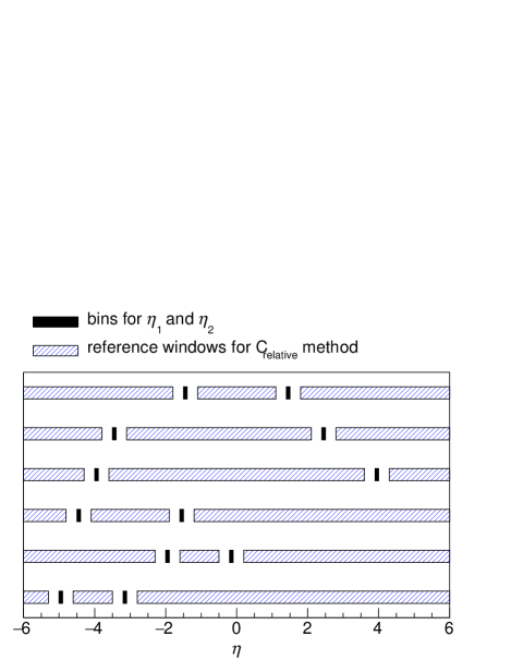
Figure 3: Illustration of reference windows in the C${}_{\textmd{relative}}$ method.

In this method, reference multiplicity is used not only for centrality cut. For a certain centrality $\varepsilon$, the expectation of reference multiplicity is denoted by $\mu_{\textmd{ref}}$. Therefore, 2PC at $\varepsilon$ can be expressed as

$$C(y_{1},y_{2};\varepsilon)=\frac{\left<n^{*}(y_{1})n^{*}(y_{2})\right>_{\varepsilon}}{\left<n^{*}(y_{1})\right>_{\varepsilon}\left<n^{*}(y_{2})\right>_{\varepsilon}}-\frac{\delta(y_{1}-y_{2})}{\mu_{\textmd{ref}}\left<n^{*}(y_{1})\right>_{\varepsilon}},$$ (20)

where $n^{*}(y_{1})\equiv N(y_{1})/\mu_{\textmd{ref}}$ and $n^{*}(y_{2})\equiv N(y_{2})/\mu_{\textmd{ref}}$, and are called ideal relative multiplicity. In a centrality window (Here, it is a reference multiplicity window in fact), if we assume that the shapes of rapidity probability distributions of different centralities are similar with each other, $\left<n^{*}(y)\right>_{\varepsilon}=\left<n^{*}(y)\right>$. Therefore, 2PC of the centrality window can be expressed as (discussed in detail in Appendix D)

$$C(y_{1},y_{2})=\frac{\left<n^{*}(y_{1})n^{*}(y_{2})\right>}{\left<n^{*}(y_{1})\right>\left<n^{*}(y_{2})\right>}-\frac{\delta(y_{1}-y_{2})}{\mu_{\textmd{ref}}\left<n^{*}(y_{1})\right>},$$ (21)

where $\left<\cdots\right>$ without a sub-index stands for the average over the centrality window. But this equation cannot be used for calculating 2PC directly, because for an event, the ideal relative multiplicities $n^{*}(y_{1})$, $n^{*}(y_{2})$ and reference multiplicity expectation $\mu_{\textmd{ref}}$ cannot be gotten experimentally.

For a measured multiplicity $N_{\textmd{ref}}$, we assume that its expectation $\mu_{\textmd{ref}}$ obeys a Gaussian distribution around $N_{\textmd{ref}}$ with a half-width $\sqrt{N_{\textmd{ref}}}$. Reference multiplicity (NO ”ideal”) is defined as $n(y)=N(y)/N_{\textmd{ref}}$. For a centrality window (reference multiplicity window), the relationship between the averages of ”relative multiplicity” and ”ideal relative multiplicity” can be expressed as (see Ref. He et al. (2016b) or Appendix D).

$$\left<n(y_{1})\right>=\left<n^{*}(y_{1})\right>,~{}~{}\left<n(y_{2})\right>=\left<n^{*}(y_{2})\right>,$$ (22)

$$\left<n(y_{1})n(y_{2})\right>=\left<n^{*}(y_{1})n^{*}(y_{1})\right>\big{(}1+\frac{1}{\left<N_{\textmd{ref}}\right>}\big{)},$$

$$\left<n^{2}(y_{1})\right>=\left<{n^{*}}^{2}(y_{1})\right>\big{(}1+\frac{1}{\left<N_{\textmd{ref}}\right>}\big{)},~{}~{}\big{<}\frac{1}{N_{\textmd{ref}}}\big{>}=\big{<}\frac{1}{\mu_{\textmd{ref}}}\big{>},$$

Taking Eq. (22) into Eq. (21), 2PC can be expressed as

$$C\left(y_{1},y_{2}\right)\!=\!\frac{\left<n(y_{1})n(y_{2})\right>}{\big{(}1\!+\!\frac{1}{\left<N_{\textmd{ref}}\right>}\big{)}\left<n(y_{1})\right>\left<n(y_{2})\right>}-\frac{\delta(y_{1}\!-\!y_{2})}{\left<n(y_{1})\right>}\big{<}\!\frac{1}{N_{\textmd{ref}}}\!\big{>},$$ (23)

where relative multiplicities $n(y_{1})\equiv N(y_{1})/N_{\textmd{ref}}$, $n(y_{2})\equiv N(y_{2})/N_{\textmd{ref}}$ and reference multiplicity $N_{\textmd{ref}}$ can be measured experimentally.

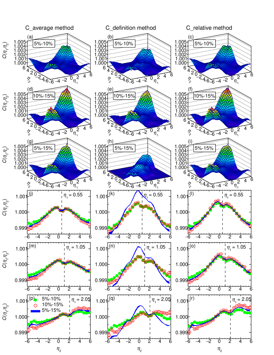
Figure 4: $C(\eta_{1},\eta_{2})$ calculated with C${}_{\textmd{average}}$Jia et al. (2016a), C${}_{\textmd{definition}}$, and C${}_{\textmd{relative}}$ method are drawn in the 1st, 2nd, and 3th columns. In subgraph (a) to (i), $C(\eta_{1},\eta_{2})$ of 5%-10%, 10%-15%, and 5%-15% are shown. In subgraph (j) to (r), for a specific $\eta_{1}$, $C(\eta_{1},\eta_{2})$ of 5%-10%, 10%-15%, and 5%-15% are shown, which can be understood as a sectional view of $C(\eta_{1},\eta_{2})$, and $\eta_{1}$ is signed with a dashed line.

IV testing the methods with ampt model and a toy granular model

In Fig. 4, for the string melting ampt model of Au+Au collisions at $\sqrt{s_{NN}}=200~{}\mathrm{GeV}$ (partonic scattering section is $3~{}\mathrm{mb}$), two-particle pseudorapidity correlation function $C(\eta_{1},\eta_{2})$ of centrality windows 5%-15%, 5%-10%, and 10%-15% are calculated with three methods. For the C${}_{\textmd{average}}$, C${}_{\textmd{definition}}$, and C${}_{\textmd{relative}}$ methods, the centrality windows are cut with multiplicity of all particles, number of charged hadrons within pseudorapidity range $[-Y,Y]$, and reference multiplicity $N_{\textmd{ref}}$, respectively.

It is seen obviously in Fig. 4 that 2PCs are all very week and around 1, and the results with different methods are similar with each other. For the C${}_{\textmd{average}}$ and C${}_{\textmd{relative}}$ methods, 2PC of 5%-15% is in the middle of 2PCs of 5%-10% and 10%-15%, and this phenomenon is more reasonable than the results in Fig. 2, which are calculated with the ratio of $\frac{\rho_{2}(\eta_{1},\eta_{2})}{\rho_{1}(\eta_{1})\rho_{1}(\eta_{2})}$ [Eq. (5)] directly. Unfortunately, the C${}_{\textmd{defintion}}$ method is suitable for the centrality windows wider than 5%. By the way, the vertical scale in Fig. 4 is different from Fig. 2. In other words, for ampt model, $C(\eta_{1},\eta_{2})$ calculated with the C${}_{\textmd{average}}$, C${}_{\textmd{definition}}$, and C${}_{\textmd{relative}}$ methods are weaker than the results in Fig. 4. In addition, they are closer to 1, and even lower than 1 (negative correlation).

On the other hand, we build a toy granular model to simulate the particle density fluctuation in rapidity. This idea is borrowed from some researches about two-pion correlation Zhang et al. (2004, 2006, 2009); Hu et al. (2015) and some similar simulation based on blast-wave model Pratt (1994); Randrup (2005); Schulc and Tomášik (2010). We assume that an event is composed of some random granules, and the particles in a granule share the same collective rapidity. Fig. 5 illustrates the particle density distributions of the granules in a random event. In Fig. 5, $N_{g}$ is the number of granules, $\mu_{g}$ is the expectation of number of particles in a granule, $\sigma_{y}$ is the half-width of the particle density distribution of a granule. Here, the rapidity of particles in a granule obeys a Gaussian distribution around the collective rapidity, and the collective rapidity distribution is borrowed from mean rapidity distribution of ampt model used above, though this assumption is rough.

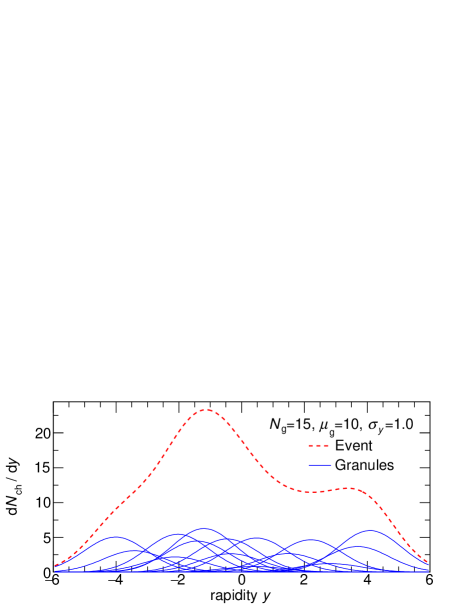
Figure 5: For the granular model, when $N_{g}$, $\mu_{g}$, and $\sigma_{y}$ are set to 15, 10, and 1.0, respectively, the probability density distributions of granules in a random event (blue full curve) and a total probability density distribution of the event (red dashed curve) are shown.

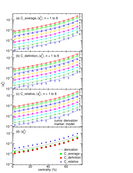
Figure 6: For the granular model with $\mu_{g}=10$ and $\sigma_{y}=1$, $\left<a_{n}^{2}\right>$ ($n$ = 1,2,$\cdots$,8) as a function of centrality are calculated with the C${}_{\textmd{average}}$, C${}_{\textmd{definition}}$, and C${}_{\textmd{relative}}$ methods and drawn as makers in (a), (b), and (c), respectively, and the corresponding deduced results are drawn with curves. In (d), comparisons between $\left<a_{0}^{2}\right>$ of derivation and these three methods are shown.

More than $2\times 10^{5}$ random events are made with the granular model (Here, $\mu_{g}=10$ and $\sigma_{y}=1.0$) by utilizing the distribution of charged hadron multiplicity ($\left|y\right|<6$) of ampt model used above. We deduced the theoretical expression of $\left<a_{n}^{2}\right>$ of the granular model in Appendix E, as shown in Eq. (65). For testing the 2PC calculation methods, $\left<a_{n}^{2}\right>$ as a function of centrality is calculated with Eq. (8) and shown in Fig. 6. It’s seen that for $n=1,2,\cdots,8$, the $\left<a_{n}^{2}\right>$ calculated with C${}_{\textmd{average}}$, C${}_{\textmd{average}}$ and C${}_{\textmd{average}}$ are similar with the results of derivation as shown in subgraph (a), (b), and (c), respectively. But for $n=0$, the differences between them can be observed as shown in subgraph (d).

In addition, we observe that $\left<a_{n}^{2}\right>$ increases with centrality in Fig. 6. It can be explained as: when the multiplicity expectation $\mu_{g}$ of granules is set, for less central events, there are less granules, which may lead to more violent fluctuation of particle density distribution.

V summary

The additional positive correlation is presented in the calculation utilizing the ratio of two-particle density $\rho_{2}(y_{1},y_{2})$ to product of single-particle densities $\rho_{1}(y_{1})\rho_{1}(y_{2})$ with ampt model of Au+Au collisions at $\sqrt{s_{NN}}=200~{}\mathrm{GeV}$. We argue that this phenomenon is due to a mixing of events of different centralities in a centrality window. In other words, this phenomenon may be caused by the centrality span. For removing or deducing the influence of centrality mixing (or centrality span), the C${}_{\textmd{definition}}$ and C${}_{\textmd{relative}}$ methods are raised. In C${}_{\textmd{definition}}$ method, the expression for calculating $C(y_{1},y_{2})$ is deduced from the normalized ratio of two-particle probability to product of single-particle probability [Eq. (2)]. In C${}_{\textmd{relative}}$ method, a relative multiplicity is introduced for unifying the events of different centralities, and the bias caused by fluctuation of reference multiplicity is modified under a Gaussian assumption. The methods are tested with ampt model and a toy granular model which simulates particle density fluctuation in rapidity. For ampt model, 2PC of 5%-15% is in the middle of 2PCs of 5%-10% and 10%-15%, as expected. For the granular model, most of results of theoretical results $\left<a_{n}^{2}\right>$ ($n$ = 1, 2, $\dots$, 8) can be reproduced with the calculation methods, though for $\left<a_{0}^{2}\right>$, the differences between the results of model and derivation can be seen.

Appendix A $\left<a_{m}a_{n}\right>$ without statistical fluctuation

In this part, we aim at why $\left<a_{m}a_{n}\right>$ without statistical fluctuation was written as $\left<a_{m}^{\textmd{obs}}a_{n}^{\textmd{obs}}\right>-\left<a_{m}^{\textmd{ran}}a_{n}^{\textmd{ran}}\right>$.

The $y$ distribution of particles in an event can be understood as the sum of statistical fluctuation and the particle density distribution without statistical fluctuation, and the latter can be seen as a collective part, and the former can be seen as a non-collective part. Before the discussion, some functions are defined as follows:

(1) $\rho(y;a_{0},a_{1},a_{2},\cdots)$: the particle density without statistical fluctuation (which can be understood as the ”collective” part).

(2) $\rho^{\textmd{ran}}(y;a_{0}^{\textmd{ran}},a_{1}^{\textmd{ran}},a_{2}^{\textmd{ran}},\cdots)$: the particle density distribution including only statistical fluctuation (which can be understood as ”non-collective”).

(3) $\rho^{\textmd{obs}}(y;a_{0}^{\textmd{obs}},a_{1}^{\textmd{obs}},a_{2}^{\textmd{obs}},\cdots)$: the particle density distribution including both event-by-event fluctuation and statistical fluctuation (which can be understood as the sum of ”collective” and ”non-collective”).

(4) $\rho_{0}(y)$: the mean single-particle density distribution.

For an event,

$$\rho^{\textmd{obs}}(y;a_{0}^{\textmd{obs}},a_{1}^{\textmd{obs}},a_{2}^{\textmd{obs}},\cdots)=\rho_{0}(y)\Big{[}1+\sum_{n}a_{n}^{\textmd{obs}}T_{n}(y)\Big{]},$$

$$\rho^{\textmd{ran}}(y;a_{0}^{\textmd{ran}},a_{1}^{\textmd{ran}},a_{2}^{\textmd{ran}},\cdots)=\rho_{0}(y)\Big{[}1+\sum_{n}a_{n}^{\textmd{ran}}T_{n}(y)\Big{]},$$

$$\rho(y;a_{0},a_{1},a_{2},\cdots)=\rho_{0}(y)\Big{[}1+\sum_{n}a_{n}T_{n}(y)\Big{]},$$ (24)

where $T_{n}(y)$ ( $n$ = 0, 1, 2, $\cdots$) are complete orthogonal basis functions. Because the observed particle density distribution $\rho^{\textmd{obs}}(y;a_{0}^{\textmd{obs}}\!\!\!,a_{1}^{\textmd{obs}}\!\!\!,\dots)$ can be understood as the sum of the $\rho(y;a_{0},a_{1},\dots)$ and pure statistical fluctuation $\rho^{\textmd{ran}}(y;a_{0}^{\textmd{ran}}\!\!\!,a_{1}^{\textmd{ran}}\!\!\!,\dots)-\rho_{0}(y)$. Hence,

$$\rho^{\textmd{obs}}(y;a_{0}^{\textmd{obs}}\!\!\!,a_{1}^{\textmd{obs}}\!\!\!,\dots)\!\!=\rho(y;a_{0},a_{1},\dots)$$

$$~{}~{}~{}~{}~{}~{}~{}~{}~{}~{}~{}~{}~{}~{}~{}~{}~{}~{}~{}~{}~{}~{}~{}~{}+\!\Big{[}\rho^{\textmd{ran}}(y;a_{0}^{\textmd{ran}}\!\!\!,a_{1}^{\textmd{ran}}\!\!\!,\dots)\!-\!\rho_{0}(y)\Big{]},~{}~{}~{}~{}~{}$$ (25)

$$\Rightarrow\sum_{n}a_{n}^{\textmd{obs}}T_{n}(y)=\sum_{n}a_{n}^{\textmd{ran}}T_{n}(y)+\sum_{n}a_{n}T_{n}(y).~{}~{}~{}$$ (26)

By utilizing the orthogonality of $T_{n}(y)$, for an event,

$$a_{n}^{\textmd{obs}}=a_{n}^{\textmd{ran}}+a_{n}.$$ (27)

It is assumed that $a_{n}^{\textmd{ran}}$ is independent of $a_{m}$, no matter whether $m=n$ or $m\neq n$. Therefore,

$$\left<a_{m}^{\textmd{obs}}a_{n}^{\textmd{obs}}\right>\!=\!\left<a_{m}^{\textmd{ran}}a_{n}^{\textmd{ran}}\right>\!+\!\left<a_{m}a_{n}\right>\!+\!\left<a_{m}^{\textmd{ran}}\right>\left<a_{n}\right>\!+\!\left<a_{n}^{\textmd{ran}}\right>\left<a_{m}\right>,$$ (28)

Besides, from the definition of $\rho^{\textmd{obs}}$ and $\rho^{\textmd{ran}}$, it is known

$$\left<\rho^{\textmd{obs}}(y;a_{0}^{\textmd{obs}},a_{1}^{\textmd{obs}},a_{2}^{\textmd{obs}},\cdots)\right>=\rho_{0}(y),$$ (29)

$$\left<\rho^{\textmd{ran}}(y;a_{0}^{\textmd{ran}},a_{1}^{\textmd{ran}},a_{2}^{\textmd{ran}},\cdots)\right>=\rho_{0}(y).$$ (30)

Taking the expressions of $\rho^{\textmd{obs}}$ and $\rho^{\textmd{ran}}$ in Eq. (24) into Eqs. (29) and (30), respectively,

$$\sum_{n}\left<a_{n}^{\textmd{obs}}\right>T_{n}(y)=0,~{}~{}\sum_{n}\left<a_{n}^{\textmd{ran}}\right>T_{n}(y)=0.$$ (31)

By utilizing the orthogonality of $T_{n}(y)$ and Eq. (27),

$$\left<a_{n}^{\textmd{obs}}\right>=0,~{}\left<a_{n}^{\textmd{ran}}\right>=0,~{}\left<a_{n}\right>=0,~{}n=0,1,2,\cdots$$ (32)

Taking Eq. (32) into Eq. (28),

$$\left<a_{m}^{\textmd{obs}}a_{n}^{\textmd{obs}}\right>=\left<a_{m}^{\textmd{ran}}a_{n}^{\textmd{ran}}\right>+\left<a_{m}a_{n}\right>.$$ (33)

Appendix B calculating $\left<a_{m}a_{n}\right>$ with two-particle rapidity correlation function

Two-particle rapidity correlation function can be expressed as

$$C(y_{1},y_{2})\!\! = \frac{\left<\rho^{\textmd{obs}}\left(y_{1};a_{1},a_{2},\cdots\right)\rho^{\textmd{obs}}\left(y_{2};a_{1},a_{2},\cdots\right)\right>}{\left<\rho^{\textmd{obs}}\left(y_{1};a_{1},a_{2},\cdots\right)\right>\left<\rho^{\textmd{obs}}\left(y_{2};a_{1},a_{2},\cdots\right)\right>}$$ (34)

$$= 1+\sum_{m,n=0}^{\infty}\left<a_{m}^{\textmd{obs}}a_{n}^{\textmd{obs}}\right>T_{m}(y)T_{n}(y).$$

For the events including only statistical fluctuation, $C^{\textmd{ran}}(y_{1},y_{2})=1$, so that

$$C^{\textmd{ran}}(y_{1},y_{2}) =1+\sum_{m,n=0}^{\infty}\left<a_{m}^{\textmd{ran}}a_{n}^{\textmd{ran}}\right>T_{m}(y)T_{n}(y)=1,$$

$$\Rightarrow~{}~{}~{}~{} \sum_{m,n=0}^{\infty}\left<a_{m}^{\textmd{ran}}a_{n}^{\textmd{ran}}\right>T_{m}(y)T_{n}(y)=0.$$ (35)

Taking Eq. (35) into Eq. (34) and utilizing Eq. (33),

$$C(y_{1},y_{2}) =\!1+\sum_{m,n=0}^{\infty}\left<a_{m}a_{n}\right>T_{m}(y)T_{n}(y),$$ (36)

$$=\!1\!+\!\!\!\sum_{m,n=0}^{\infty}\!\!\!\left<a_{m}a_{n}\right>\frac{T_{m}(y_{1})T_{n}(y_{2})\!+\!T_{m}(y_{2})T_{n}(y_{1})}{2}$$

By utilizing the normalization and orthogonality expressed as $\frac{1}{Y^{2}}\int_{-Y}^{Y}\int_{-Y}^{Y}T_{m}(y_{1})T_{n}(y_{2})dy_{1}dy_{2}=\delta_{mn}$, integrating both sides of Eq. (36), we can get

$$\frac{1}{Y^{2}}\int_{-Y}^{Y}\int_{-Y}^{Y}\left[C(y_{1},y_{2})-1\right]T_{\mu}(y_{1})T_{\nu}(y_{2})dy_{1}dy_{2}$$ (37)

$$= \sum_{m,n=0}^{\infty}\left<a_{m}a_{n}\right>\frac{\delta_{m\mu}\delta_{n\nu}+\delta_{m\nu}\delta_{n\mu}}{2}=\left<a_{\mu}a_{\nu}\right>,$$

which is equivalent to Eq. (8).

Appendix C positive correlation caused by centrality span

In this part, we explain where the additional positive correlation is from, when 2PC is calculated with Eq. (5). In a centrality window, we assume that the 2PCs of narrow sub-windows are equal to each other. For example, in the centrality window 10%-20%, we assume

$$C(y_{1},y_{2};10\%)\!=\!C(y_{1},y_{2};11\%)\!=\!\cdots\!=\!C(y_{1},y_{2};20\%)\!=\!c.$$ (38)

Here, $C(y_{1},y_{2};\varepsilon)$ stands for the 2PC of a centrality bin around $\varepsilon$, the bin widths are all equal to 1%, $c$ is a constant. Hence,

$$~{}~{}~{}\begin{aligned} &\left.\rho_{2}(y_{1},y_{2};10\%)\middle/\big{[}\rho_{1}(y_{1};10\%)\rho_{1}(y_{2};10\%)\big{]}\right.\\ =&\left.\rho_{2}(y_{1},y_{2};11\%)\middle/\big{[}\rho_{1}(y_{1};11\%)\rho_{1}(y_{2};11\%)\big{]}\right.\\ =&~{}~{}~{}~{}~{}~{}~{}~{}~{}~{}~{}~{}~{}\cdots\\ =&\left.\rho_{2}(y_{1},y_{2};20\%)\middle/\big{[}\rho_{1}(y_{1};20\%)\rho_{1}(y_{2};20\%)\big{]}\right.=c.\end{aligned}~{}~{}~{}$$ (39)

$$\Rightarrow\frac{\left<\rho_{2}(y_{1},y_{2};\varepsilon)\right>}{\left<\rho_{1}(y_{1};\varepsilon)\rho_{1}(y_{2};\varepsilon)\right>}=\frac{\left.\sum_{\varepsilon}\rho_{2}(y_{1},y_{2};\varepsilon)\right.}{\left.\sum_{\varepsilon}\rho_{1}(y_{1};\varepsilon)\rho_{1}(y_{2};\varepsilon)\right.}=c.~{}~{}~{}~{}~{}$$ (40)

Besides, we assume that

$$\rho_{1}(y_{1};10\%)>\rho_{1}(y_{1};11\%)>\cdots>\rho_{1}(y_{1};20\%),~{}~{}~{}$$ (41)

$$\rho_{1}(y_{2};10\%)>\rho_{1}(y_{2};11\%)>\cdots>\rho_{1}(y_{2};20\%).~{}~{}~{}$$ (42)

Therefore,

$$~{}~{}\left<\rho_{1}(y_{1};\varepsilon)\right>\left<\rho_{1}(y_{2};\varepsilon)\right><\left<\rho_{1}(y_{1};\varepsilon)\rho_{1}(y_{2};\varepsilon)\right>,$$ (43)

$$\Rightarrow ~{}~{}~{}\frac{\left<\rho_{2}(y_{1},y_{2};\varepsilon)\right>}{\left<\rho_{1}(y_{1};\varepsilon)\right>\left<\rho_{1}(y_{2};\varepsilon)\right>}>\frac{\left<\rho_{2}(y_{1},y_{2};\varepsilon)\right>}{\left<\rho_{1}(y_{1};\varepsilon)\rho_{1}(y_{2};\varepsilon)\right>},~{}~{}~{}$$ (44)

$$\Rightarrow ~{}~{}~{}~{}~{}~{}~{}~{}C(y_{1},y_{2};10\%\!\!-\!\!20\%)>c,$$ (45)

where, $\left<\cdots\right>$ stands for the average over all the centrality bins within 10%-20%. By comparing Eqs. (38) and (45), we argue that some additional positive correlation may be caused by a wide centrality span.

It is notable that in the derivation above, this proposition is used

$$\left.\begin{aligned} a_{1}>a_{2}>\cdots>a_{n}>0\\ b_{1}>b_{2}>\cdots>b_{n}>0\end{aligned}\right\}\Rightarrow\left<a_{i}\right>\left<b_{i}\right><\left<a_{i}b_{i}\right>.$$ (46)

It is proved as follows.

$$\left<a_{i}b_{i}\right>>\left<a_{i}\right>\left<b_{i}\right>$$ (47)

$$\Leftrightarrow n\sum_{i=1}^{n}a_{i}b_{i}-\sum_{i=1}^{n}\sum_{j=1}^{n}a_{i}b_{j}>0$$ (48)

$$\Leftrightarrow \left\{\!\begin{aligned} &a_{1}(b_{1}\!-\!b_{1})\!+\!a_{1}(b_{1}\!-\!b_{2})\!+\!\cdots\!+\!a_{1}(b_{1}\!-\!b_{n})\\ +&a_{2}(b_{2}\!-\!b_{1})\!+\!a_{2}(b_{2}\!\!-b_{2})\!+\!\cdots+a_{2}(b_{2}\!\!-b_{n})\\ +&~{}~{}~{}~{}~{}~{}~{}~{}~{}~{}~{}~{}~{}~{}~{}\cdots\\ +&a_{n}(b_{n}\!-\!b_{1})\!+\!a_{n}(b_{n}\!-\!b_{2})\!+\!\cdots\!+\!a_{n}(b_{n}\!-\!b_{n})\!>\!0\end{aligned}\right.$$ (49)

$$\Leftrightarrow \sum_{i=1}^{n}\sum_{j=i+1}^{n}(a_{i}-a_{j})(b_{i}-b_{j})>0$$ (50)

$$\Leftarrow \left\{\begin{aligned} a_{1}>a_{2}>a_{3}>\cdots>a_{n}>0\\ b_{1}>b_{2}>b_{3}>\cdots>b_{n}>0\end{aligned}\right.~{}~{}~{}~{}\textmd{proved.}$$ (51)

Appendix D detailed derivation of C${}_{\textmd{relative}}$ method

In this section, some detailed derivations about the C${}_{\textmd{relative}}$ method are added. For a certain centrality $\varepsilon$, $C(y_{1},y_{2};\varepsilon)$ can be expressed as Eq. (20), just like

$$C(y_{1},y_{2};\varepsilon) =\frac{\left<n^{*}(y_{1})n^{*}(y_{2})\right>_{\varepsilon}}{\left<n^{*}(y_{1})\right>_{\varepsilon}\left<n^{*}(y_{2})\right>_{\varepsilon}}-\frac{\delta(y_{1}-y_{2})}{\mu_{\textmd{ref}}\left<n^{*}(y_{1})\right>_{\varepsilon}}$$ (52)

$$=\frac{\left<\big{[}n^{*}(y_{1})-\frac{1}{\mu_{\textmd{ref}}}\delta(y_{1}-y_{2})\big{]}n^{*}(y_{2})\right>_{\varepsilon}}{\left<n^{*}(y_{1})\right>_{\varepsilon}\left<n^{*}(y_{2})\right>_{\varepsilon}},$$

where $n^{*}(y_{1})\equiv N(y_{1})/\mu_{\textmd{ref}}$ and $n^{*}(y_{2})\equiv N(y_{2})/\mu_{\textmd{ref}}$. It is equivalent to

$$C(y_{1},y_{2};\textmd{window})\left<n^{*}(y_{1})\right>_{\varepsilon}\left<n^{*}(y_{2})\right>_{\varepsilon}$$ (53)

$$=\Big{<}\big{[}n^{*}(y_{1})-\frac{\delta(y_{1}-y_{2})}{\mu_{\textmd{ref}}}\big{]}n^{*}(y_{2})\Big{>}_{\varepsilon}.$$

Here, we assume $C(y_{1},y_{2};\varepsilon)$ of different centralities in the window are equal to each other, and denoted by $C(y_{1},y_{2};\textmd{window})$. If we assume the shapes of single-particle probability density distribution in rapidity of different centralities are similar with each other,

$$\left<n^{*}(y)\right>_{\varepsilon}=\left<n^{*}(y)\right>$$ (54)

where $\left<\cdots\right>$ WITHOUT a sub-index $\varepsilon$ stands for the average over the whole centrality window, and it is equivalent to $\int\cdots f(\varepsilon)d\varepsilon$, where $f(\varepsilon)$ is the centrality probability density distribution in the window. Averaging both sides of Eq. (53) over the events in the window and utilizing Eq. (54),

$$C(y_{1},y_{2};\textmd{window})=\frac{\Big{<}\big{[}n^{*}(y_{1})-\frac{\delta(y_{1}-y_{2})}{\mu_{\textmd{ref}}}\big{]}n^{*}(y_{2})\Big{>}}{\left<n^{*}(y_{1})\right>\left<n^{*}(y_{2})\right>}.$$ (55)

It is equivalent to Eq. (21).

On the other hand, under the Gaussian assumption, we deduce the relationship between the averages about ideal relative multiplicity $n^{*}(y)$ and relative multiplicity $n(y)$ as follows. Here, for a measured $N_{\textmd{ref}}$, we assume that $\mu_{\textmd{ref}}$ obeys a Gaussian distribution as

$$G\left(\mu_{\textmd{ref}};N_{\textmd{ref}},\sqrt{N_{\textmd{ref}}}\right)\!=\!\frac{1}{\sqrt{2\pi N_{\textmd{ref}}}}\exp\Big{[}\!-\!\frac{\left(\mu_{\textmd{ref}}\!-\!N_{\textmd{ref}}\right)^{2}}{2N_{\textmd{ref}}}\Big{]},$$ (56)

where $\mu_{\textmd{ref}}$ and $\sqrt{N_{\textmd{ref}}}$ can be understood as the truth value and statistical error of a measured $N_{\textmd{ref}}$, respectively. It is worth to note that the Gaussian approximation is not suitable enough for the most central events such as 0%-5%, and it is discussed in detail in Ref. He et al. (2016b). When the most central windows are avoided, under the Gaussian assumption,

$$\big{<}\frac{\mu_{\textmd{ref}}}{N_{\textmd{ref}}}\big{>}\! = \!\!\int\!\!\!\int\!\!\!\frac{\mu_{\textmd{ref}}}{N_{\textmd{ref}}}G\left(\mu_{\textmd{ref}};N_{\textmd{ref}},\sqrt{N_{\textmd{ref}}}\right)\!h\left(N_{\textmd{ref}}\right)dN_{\textmd{ref}}d\mu_{\textmd{ref}}$$ (57)

$$= 1,$$

$$\big{<}\frac{\mu_{\textmd{ref}}^{2}}{N_{\textmd{ref}}^{2}}\big{>}\! = \!\!\int\!\!\!\int\!\!\!\frac{\mu_{\textmd{ref}}^{2}}{N_{\textmd{ref}}^{2}}G\left(\mu_{\textmd{ref}};N_{\textmd{ref}},\sqrt{N_{\textmd{ref}}}\right)h\left(N_{\textmd{ref}}\right)dN_{\textmd{ref}}d\mu_{\textmd{ref}}$$ (58)

$$= 1+\frac{1}{\left<N_{\textmd{ref}}\right>},$$

where $h\left(N_{\textmd{ref}}\right)$ is the probability density function of $N_{\textmd{ref}}$ in a centrality window (in fact, it is a $N_{\textmd{ref}}$ window). We define an ideal relative reference multiplicity $n_{\textmd{ref}}\equiv N_{\textmd{ref}}/\mu_{\textmd{ref}}$, and Eq. (58) can be simplified to $\big{<}\frac{1}{n_{\textmd{ref}}}\big{>}=1$ and $\big{<}\frac{1}{n_{\textmd{ref}}^{2}}\big{>}=1+\frac{1}{\left<N_{\textmd{ref}}\right>}$.

By utilizing Eqs. (57) and (58), the relationship between $\left<n(y_{1})\right>$, $\left<n(y_{2})\right>$, $\left<n(y_{1})n(y_{2})\right>$, $\left<n^{2}(y_{1})\right>$, $\left<\frac{1}{N_{\textmd{ref}}}\right>$ and $\left<n^{*}(y_{1})\right>$, $\left<n^{*}(y_{2})\right>$, $\left<n^{*}(y_{1})n^{*}(y_{2})\right>$, $\left<{n^{*}}^{2}(y_{1})\right>$, $\left<\frac{1}{n_{\textmd{ref}}}\right>$ can be expressed as

$$\left<n(y_{1})\right>=\left<\frac{N(y_{1})}{\mu_{\textmd{ref}}}\frac{\mu_{\textmd{ref}}}{N_{\textmd{ref}}}\right>=\left<n^{*}(y_{1})\frac{1}{n_{\textmd{ref}}}\right>=\left<n^{*}(y_{1})\right>\left<\frac{1}{n_{\textmd{ref}}}\right>=\left<n^{*}(y_{1})\right>,$$

$$\left<n(y_{1})n(y_{2})\right>=\left<\frac{N(y_{1})}{\mu_{\textmd{ref}}}\frac{N(y_{2})}{\mu_{\textmd{ref}}}\frac{\mu_{\textmd{ref}}^{2}}{N_{\textmd{ref}}^{2}}\right>=\left<\frac{n^{*}(y_{1})n^{*}(y_{2})}{n_{\textmd{ref}}^{2}}\right>=\left<n^{*}(y_{1})n^{*}(y_{2})\right>\big{(}1+\frac{1}{\left<N_{\textmd{ref}}\right>}\big{)},$$

$$\left<n^{2}(y_{1})\right>=\left<\frac{N^{2}(y_{1})}{\mu_{\textmd{ref}}^{2}}\frac{\mu_{\textmd{ref}}^{2}}{N_{\textmd{ref}}^{2}}\right>=\left<{n^{*}}^{2}(y_{1})\right>\left<\frac{1}{n_{\textmd{ref}}^{2}}\right>=\left<{n^{*}}^{2}(y_{1})\right>\big{(}1+\frac{1}{\left<N_{\textmd{ref}}\right>}\big{)},$$

$$\left<\frac{1}{N_{\textmd{ref}}}\right>=\left<\frac{1}{\mu_{\textmd{ref}}}\frac{\mu_{\textmd{ref}}}{N_{\textmd{ref}}}\right>=\left<\frac{1}{\mu_{\textmd{ref}}}\right>\left<\frac{1}{n_{\textmd{ref}}}\right>=\left<\frac{1}{\mu_{\textmd{ref}}}\right>.$$ (59)

Similarly, $\langle n(y_{2})\rangle=\langle n^{*}(y_{2})\rangle$. Here, the correlation between $n^{*}(y_{1})$ (or $n^{*}(y_{2})$) and $n_{\textmd{ref}}$ is ignored. Taking Eq. (59) into Eq. (55) and ignoring the correlation between $n^{*}(y_{1})$ (or $n^{*}(y_{2})$) and $\mu_{\textmd{ref}}$, the expression of 2PC of the C${}_{\textmd{relative}}$ method [Eq. (23)] can be gotten.

Appendix E theoretical expression of $C(y_{1},y_{2})$ and $\left<a_{m}a_{n}\right>$ of granular model

$C(y_{1},y_{2})$ and $\left<a_{m}a_{n}\right>$ of the granular model are deduced as follows. In this part, $G(x;\mu,\sigma)$ stands for a Gaussian function of $x$ with an expectation $\mu$ and standard deviation $\sigma$. In this toy granular model, we assume:

(1) number of particles $m_{g}$ in a granule obeys a Gaussian function $G(m_{g};\mu_{g},\sqrt{\mu_{g}})$;

(2) the normalized collective rapidity probability distribution function is denoted by $f_{g}(y_{g})$;

(3) rapidity of particle in a granule obeys a Gaussian function around the collective rapidity $y_{g}$, which is denoted by $G(y;y_{g},\sigma_{y})$.

For an event with $N_{g}$ granules, when the granular multiplicity $m_{g_{i}}$ and the granule rapidity $y_{g_{i}}$ (where the sub-index $i=1,2,\dots,N_{g}$ is the ordinal number of granules) are known, the single- and double-particle density distributions can be expressed as

$$\rho_{1}(y;m_{g_{1}},m_{g_{2}},\cdots,y_{g_{1}},y_{g_{2}},\cdots) = \sum_{i=1}^{N_{g}}m_{g_{i}}G\left(y;y_{g_{i}},\sigma_{y}\right),$$ (60)

$$\rho_{2}(y_{1},y_{2};m_{g_{1}},m_{g_{2}},\cdots,y_{g_{1}},y_{g_{2}},\cdots) = \sum_{i=1}^{N_{g}}\sum_{j=1}^{N_{g}}m_{g_{i}}m_{g_{j}}G\left(y;y_{g_{i}},\sigma_{y}\right)G\left(y;y_{g_{j}},\sigma_{y}\right).$$ (61)

When the granule-multiplicity expectation $\mu_{g}$ and the granular collective rapidity distribution $f_{g}(y_{g})$ are both known,

$$\begin{aligned} &\rho_{1}(y)=\!\!\int\!\!\cdots\!\!\int\!\!\bigg{[}\sum_{i=1}^{N_{g}}m_{g_{i}}G\left(y;y_{g_{i}},\sigma_{y}\right)\bigg{]}\prod_{j=1}^{N_{g}}f_{g}(y_{g_{j}})G\left(m_{g_{j}};\mu_{g},\sqrt{\mu_{g}}\right)dy_{g_{j}}dm_{g_{j}}=N_{g}\mu_{g}\int G\left(y;y_{g},\sigma_{y}\right)f_{g}(y_{g})dy_{g},\end{aligned}$$ (62)

$$\begin{aligned} \rho_{2}(y_{1},y_{2})=&\!\!\int\!\!\cdots\!\!\int\!\!\sum_{i=1}^{N_{g}}\sum_{j=1}^{N_{g}}m_{g_{i}}m_{g_{j}}G\left(y_{1};y_{g_{i}},\sigma_{y}\right)G\left(y_{2};y_{g_{j}},\sigma_{y}\right)\prod_{k=1}^{N_{g}}f_{g}(y_{g_{k}})G\left(m_{g_{k}};\mu_{g},\sqrt{\mu_{g}}\right)dy_{g_{k}}dm_{g_{k}}\\ =&N_{g}\left(N_{g}-1\right)\mu_{g}^{2}\int G\left(y_{1};y_{g},\sigma_{y}\right)f_{g}(y_{g})dy_{g}\int G\left(y_{2};y_{g},\sigma_{y}\right)f_{g}(y_{g})dy_{g}\\ &+N_{g}\left(\mu_{g}^{2}+\mu_{g}\right)\int G\left(y_{1};y_{g},\sigma_{y}\right)G\left(y_{2};y_{g},\sigma_{y}\right)f_{g}(y_{g})dy_{g}.\end{aligned}$$ (63)

The theoretical expression of 2PC of the granular model is calculated as the ratio of $\rho_{2}(y_{1},y_{2})$ to $\rho_{1}(y_{1})\rho_{1}(y_{2})$ (Here, the number of granules $N_{g}$ is a constant),

$$C(y_{1},y_{2})=\frac{\rho_{2}(y_{1},y_{2})}{\rho_{1}(y_{1})\rho_{1}(y_{2})}=\frac{1}{N_{g}}\left(1+\frac{1}{\mu_{g}}\right)\frac{\int G\left(y_{1};y_{g},\sigma_{y}\right)G\left(y_{2};y_{g},\sigma_{y}\right)f_{g}(y_{g})dy_{g}}{\int G\left(y_{1};y_{g},\sigma_{y}\right)f_{g}(y_{g})dy_{g}\int G\left(y_{2};y_{g},\sigma_{y}\right)f_{g}(y_{g})dy_{g}}+1-\frac{1}{N_{g}}.$$ (64)

Taking Eq. (64) into Eq. (8), $\left<a_{m}a_{n}\right>$ can be expressed as

$$\left<a_{m}a_{n}\right>=\frac{1+\mu_{g}}{\langle M\rangle Y^{2}}\int_{-Y}^{Y}\int_{-Y}^{Y}\frac{\int G\left(y_{1};y_{g},\sigma_{y}\right)G\left(y_{2};y_{g},\sigma_{y}\right)f_{g}(y_{g})dy_{g}}{\int G\left(y_{1};y_{g},\sigma_{y}\right)f_{g}(y_{g})dy_{g}\int G\left(y_{2};y_{g},\sigma_{y}\right)f_{g}(y_{g})dy_{g}}T_{m}(y_{1})T_{n}(y_{2})dy_{1}dy_{2}-\frac{2\delta_{m0}\delta_{n0}}{N_{g}}.$$ (65)

The factor $\frac{1}{N_{g}}\left(1+\frac{1}{\mu_{g}}\right)$ in Eq. (64) can be written as $\frac{1+\mu_{g}}{\langle M\rangle}$, just like the ratio in Eq. (65). Here $\langle M\rangle=N_{g}\mu_{g}$ can be understood as mean multiplicity.

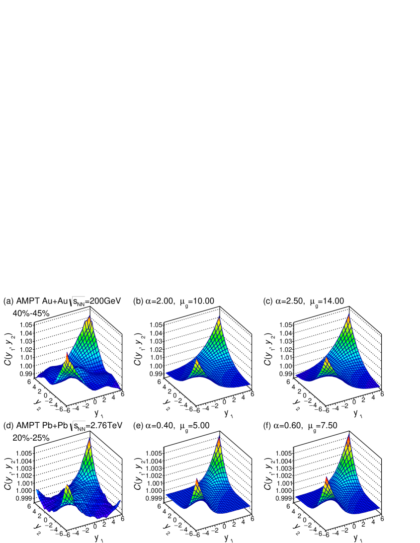
Figure 7: Comparisons between $C(y_{1},y_{2})$ of ampt model and the deduced results of granular model [Eq. (70)]. For Au+Au collision at $\sqrt{s_{NN}}$ = 200 GeV, 2PC for the centrality window 40%-45% are shown in subgraph (a). In subgraph (b) and (c), 2PC are calculated with Eq. (70) with $\sigma_{\textmd{event},y}$ and $\langle M\rangle$ which are gotten from corresponding data in (a), and the parameters $\mu_{g}$ and $\alpha$ are adjusted and signed in the subgraphs. The similar calculations are made for Pb+Pb collisions at $\sqrt{s_{NN}}$ = 2.76 TeV, and the results are shown in (d), (e), and (f).

In addition, for simplifying the expression of $\left<a_{m}a_{n}\right>$, we assume that granule-rapidity distribution $f_{g}(y_{y})$ is a Gaussian function with an expectation 0 and a standard deviation $\sigma_{y_{g}}$, denoted by

$$f_{g}\left(y_{g};\sigma_{y_{g}}\right)=\frac{1}{\sqrt{2\pi}\sigma_{y_{g}}}\exp{\left(-\frac{y_{g}^{2}}{2\sigma_{y_{g}}^{2}}\right)}.$$ (66)

For simplifying the following expressions, we define $\alpha\equiv\sigma_{y}^{2}/\sigma_{y_{g}}^{2}$, which can be understood as a relative width of granule in rapidity. Taking Eq. (66) into Eqs. (64) and (65), $C(y_{1},y_{2})$ and $\left<a_{m}a_{n}\right>$ can be expressed as

$$C(y_{1},y_{2})=\frac{1}{\langle M\rangle}\left\{\frac{(1+\mu_{g})(\alpha+1)}{\sqrt{\left(\alpha+2\right)\alpha}}\exp\left[-\frac{y_{1}^{2}+y_{2}^{2}-2(\alpha+1)y_{1}y_{2}}{2\sigma_{y_{g}}^{2}\alpha(\alpha+1)(\alpha+2)}\right]-\mu_{g}\right\}+1,$$ (67)

$$\left<a_{m}a_{n}\right>=\frac{1+\mu_{g}}{\langle M\rangle}\frac{1}{Y^{2}}\int\frac{\alpha+1}{\sqrt{(\alpha+2)\alpha}}\exp\left[{-\frac{y_{1}^{2}+y_{2}^{2}-2(\alpha+1)y_{1}y_{2}}{2\sigma_{y_{g}}^{2}\alpha(\alpha+1)(\alpha+2)}}\right]T_{n}(y_{1})T_{n}(y_{2})dy_{1}dy_{2}-\frac{2\mu_{g}\delta_{m0}\delta_{n0}}{\left<M\right>}.$$ (68)

Under the Gaussian assumption of $f_{g}(y_{g})$, the rapidity distribution in events can be expressed as

$$\frac{dN_{\textmd{ch}}}{dy}\propto\int G(y;y_{g},\sigma_{y})f_{g}(y_{g};\sigma_{y_{g}})dy_{g}=\frac{1}{\sqrt{2\pi}\sqrt{\alpha+1}\sigma_{y_{g}}}\exp\left[-\frac{y^{2}}{2(\alpha+1)\sigma_{y_{g}}^{2}}\right],$$ (69)

which can be understood as a Gaussian distribution with a half-width $\sigma_{\textmd{event},y}=\sqrt{\alpha+1}\sigma_{y_{g}}$. Taking $\sigma_{\textmd{event},y}$ into Eqs. (67) and (68), $C(y_{1},y_{2})$ and $\left<a_{m}a_{n}\right>$ are expressed respectively as

$$C(y_{1},y_{2})=\frac{1}{\langle M\rangle}\left\{\frac{(1+\mu_{g})(\alpha+1)}{\sqrt{\left(\alpha+2\right)\alpha}}\exp\left[-\frac{y_{1}^{2}+y_{2}^{2}-2(\alpha+1)y_{1}y_{2}}{2\sigma_{\textmd{event},y}^{2}\alpha(\alpha+2)}\right]-\mu_{g}\right\}+1,$$ (70)

$$\left<a_{m}a_{n}\right>=\frac{1+\mu_{g}}{\langle M\rangle}\frac{1}{Y^{2}}\int\frac{\alpha+1}{\sqrt{(\alpha+2)\alpha}}\exp\left[{-\frac{y_{1}^{2}+y_{2}^{2}-2(\alpha+1)y_{1}y_{2}}{2\sigma_{\textmd{event},y}^{2}\alpha(\alpha+2)}}\right]T_{n}(y_{1})T_{n}(y_{2})dy_{1}dy_{2}-\frac{2\mu_{g}\delta_{m0}\delta_{n0}}{\left<M\right>},$$ (71)

where the $\sigma_{\textmd{event},y}$ and $\left<M\right>$ can be measured as the standard deviation of rapidity and mean charged particle multiplicity, respectively. For ampt model of Au+Au collisions at $\sqrt{s_{NN}}$ = 200 GeV (centrality 40%-45%) and Pb+Pb collisions at $\sqrt{s_{NN}}$ = 2.76 TeV (centrality 20%-25%), we try to reproduce the $C(y_{1},y_{2})$ by adjusting the parameters $\alpha$ and $\mu_{g}$, and the results are shown in Fig. 7.