A formula for the Entropy of the Convolution of Gibbs probabilities on the circle

Abstract.

Consider the transformation $T:S^{1}\to S^{1}$, such that $T(x)=2\,x$ (mod 1), and where $S^{1}$ is the unitary circle. Suppose $J:S^{1}\to\mathbb{R}$ is Hölder continuous and positive, and moreover that, for any $y\in S^{1}$, we have that $\sum_{x\,\,\text{such that}\,\,\,T(x)=y}\,J(x)=1.$

We say that $\rho$ is a Gibbs probability for the Hölder continuous potential $\log J$, if $\mathcal{L}_{\log J}^{*}\,(\rho)=\rho,$ where $\mathcal{L}_{\log J}$ is the Ruelle operator for $\log J$. We call $J$ the Jacobian of $\rho$.

Suppose $\nu=\mu_{1}*\mu_{2}$ is the convolution of two Gibbs probabilities $\mu_{1}$ and $\mu_{2}$ associated, respectively, to $\log J_{1}$ and $\log J_{2}$. We show that $\nu$ is also Gibbs and its Jacobian $\tilde{J}$ is given by $\tilde{J}(u)=\int J_{1}(u-x)d\mu_{2}(x)$

In this case, the entropy $h(\nu)$ is given by the expression

$$h(\nu)=-\int\,[\,\,\int\,\log\,(\,\int J_{1}(r+s-x)d\mu_{2}(x)\,)\,d\mu_{2}(r)\,\,]\,\,d\mu_{1}(s).$$

For a fixed $\mu_{2}$ we consider differentiable variations $\mu_{1}^{t}$, $t\in(-\epsilon,\epsilon)$, of $\mu_{1}$ on the Banach manifold of Gibbs probabilities, where $\mu_{1}^{0}=\mu_{1}$, and we estimate the derivative of the entropy $h(\mu_{1}^{t}*\mu_{2})$ at $t=0$.

We also present an expression for the Jacobian of the convolution of a Gibbs probability $\rho$ with the invariant probability with support on a periodic orbit of period two. This expression is based on the Jacobian of $\rho$ and two Radon-Nidodym derivatives.

Inst. de Matemática, UFRGS - Porto Alegre, Brasil

1. Introduction

Consider the $2\,x$ (mod 1) transformation $T$ on the unitary circle $S^{1}$.

All expressions of the form $x+y$ below are consider (mod 1).

Given two probabilities $\eta$ and $\mu$ on $S^{1}$ the convolution $\nu\,=\,\eta*\mu$ is the probability such that for any Borel set $A$ we have

$$\nu(A)=(\eta*\mu)(A)=\int\,\mu(A-x)\,d\eta(x).$$

This is the same as saying that for any continuous function $\phi$

$$\int\phi(z)d\nu(z)=\int\,(\int\,\phi(y+x)\,d\mu(y))\,d\,\eta(x).$$

Note that if $\mu$ is the Lebesgue probability on $S^{1}$ then, for any $\nu$ we get $\mu*\nu=\mu$ (just change coordinates).

On the other hand if $\mu=\delta_{0}$, then, for any $\nu$ we have that $\mu*\nu=\nu$.

Suppose $\mu$ and $\eta$ are $T$ invariant.

Note that for any continuous $\phi$

$$\int(\phi\circ T)(z)\,\ d\nu(z)=\int\,(\int\,(\phi\circ T)(x+y)\,d\mu(y))\,d\,\eta(x)=\,\,\,$$

$$\int\,(\int\,(\phi(\,T(x)+T(y)\,)\,d\mu(y))\,d\,\eta(x)=$$

$$\int\,(\int\,(\phi(\,T(x)+y\,)\,d\mu(y))\,d\,\eta(x)=$$

$$\int\,(\int\,(\phi(\,x+y\,)\,d\mu(y))\,d\,\eta(x)=\int\phi(z)d\nu(z).$$

Then, it follows that $\nu$ is also $T$-invariant.

The convolution operation is commutative.

A very important contribution to the topic of convolution of invariant probabilities on the circle is [6]. By means of combinatorial techniques it was proved there, among other things, the convergence of the n-convolution of positive entropy measures for the Lebesgue measure. They also show that convolution does not decrease entropy (increase in most of the examples). The proofs of our results have a different nature (and they are for a particular family of probabilities).

Related results concerning convolution are [4], [10], [11] and [12].

Definition 1.

The Jacobian of an invariant measure $\rho$ is the measurable transformation $J_{\rho}$ such that

$$\rho(T(A))=\int_{A}J_{\rho}^{\,-1}d\rho,$$

for any Borel set $A$ such that $T|_{A}$ is injective (see the paragraphs before Proposition 3.4 in [18]).

The role of $J_{\rho}^{\,-1}$ is to provide a formula for the change of variables on the inverse branches of $T$.

A more elegant form of expressing this property for $J_{\rho}^{\,-1}$ (in the particular case which is the main interest of our paper ) is via the Ruelle operator. We begin with the ”Jacobian” and a posteriori we get the probability. We point out that the Jacobian in [18] is the inverse of what we call Jacobian here.

We assume from now on that $J:S^{1}\to\mathbb{R}$ is at least continuous and positive, and such that, for any $y$ we have that

$$\sum_{x\,\,\text{such that}\,\,\,T(x)=y}\,J(x)=1.$$

Given $J$ as above the Ruelle operator $\mathcal{L}_{\log J}$ acts on continuous functions $\varphi$ on the following way: $\mathcal{L}_{\log J}(\varphi)=\phi$, where

$$\phi(y)=\sum_{x\,\,\text{such that}\,\,\,T(x)=y}\,J(x)\,\varphi(x).$$

The dual $\mathcal{L}_{\log J}^{*}$ of $\mathcal{L}_{\log J}$ acts on probabilities.

Definition 2.

We say that $\rho$ is a Gibbs probability (or, a $g$-measure, where $g=\log J$) for the continuous function $J$ if

$$\mathcal{L}_{\log J}^{*}\,(\rho)=\rho.$$

The entropy of $\rho$ is given by the Rokhlin formula: $-\int\log Jd\rho$ (see for instance section 9.7 in [21]). The probability $\rho$ is the equilibrium probability (maximize pressure) for the potential $\log J$ (see Proposition 3.4 in [14]).

The Jacobian $J_{\rho}$ of $\rho$ according to definition 1 agrees with the above $J$.

In this way is natural to call $J$ the Jacobian of $\rho$.

As an example we mention that for the transformation $T(x)$= $2x$ (mod $1$) the Lebesgue probability has Jacobian $J$ constant equal to $1/2$.

If $J$ is just continuous it is possible that exists more than one fixed point probability for $\mathcal{L}_{\log J}^{*}$ (see [2] and [17]). If $J$ is Hölder the fixed point probability is unique.

General references for Jacobians and Thermodynamics Formalism are [21], [13], [14], [15] and [19]. We use the dynamics of the doubling map on an essential way. The possible extension to expanding transformations on the circle would require a good meaning for translation on the circle which is at the same time compatible with the distance among preimages of a general point.

In the section 2 we will consider convolution of two Gibbs probabilities. We estimate the entropy of the convolution of two Gibbs probabilities (see Theorem 3). We also show for the case of Gibbs probabilities that, if $\nu=\mu_{1}*\mu_{2}$, then, $h(\nu)\geq h(\mu_{2})$ (see Theorem 6). This result appears in a more general setting in [6]. We do not use here the Hausdorff dimension as a tool in our proof.

We will present in section 3 an explicit expression for the Jacobian of the probability obtained by the convolution of a Gibbs probability and a periodic orbit of period two (see expression (14)).

We also show examples of Gibbs probabilities $\mu$ where the convolution of $\mu$ with a periodic orbit of period two results in the same probability $\mu$ (see the class of potentials $\mathcal{S}$ defined by expression (21)).

In section 4 we analyze the following problem: for a fixed $\mu_{2}$ consider differentiable variations $\mu_{1}^{t}$, $t\in(-\epsilon,\epsilon)$, of $\mu_{1}$ on the Banach manifold of Gibbs probabilities, where $\mu_{1}^{0}=\mu_{1}$. How can one estimate the derivative of the entropy $h(\mu_{1}^{t}*\mu_{2})$ at $t=0$? On this direction see Proposition 12.

In the appendix we consider the following problem: suppose $J_{1}$ and $J_{2}$ are the Hölder Jacobians and they are such that: $J_{2}\geq J_{1}$, when $J_{1}\geq 1/2$, and $J_{2}\leq J_{1}$, when $J_{1}\leq 1/2$. Denote $\mu_{i}$ the Gibbs probability associated to the potential $\log J_{i}$, $i=1,2$. We show that $h(\mu_{1})\geq h(\mu_{2})$ (see Proposition 13). This problem is related to questions raised in section 3.

The PhD thesis [20] and [1] consider several properties for the convolution of invariant probabilities for the symbolic space setting. An appropriate structure have to be considered for replacing the sum translation on the circle. These works do not consider results similar to ours.

We thanks L. Cioletti, P. Giulietti and B. Uggioni for helpful conversations on the topic of convolution of invariant probabilities.

2. Convolution of Gibbs probabilities

Suppose $J_{2}$ is a Hölder Jacobian and $J_{1}$ is a Jacobian which is just continuous. As we said $J_{i}:S^{1}\to\mathbb{R}$, $i=1,2$, are such that $\mathcal{L}_{\log J_{i}}^{*}(\mu_{i})=\mu_{i}$. The probability $\mu_{2}$ is invariant, ergodic and has support on $S^{1}$.

We want to estimate analytical properties of the probability $\nu=\mu_{1}*\mu_{2}$.

A natural question is to ask if there exists an explicit expression for the Jacobian $\tilde{J}$, such that,

$$\mathcal{L}_{\log\tilde{J}}^{*}\,(\nu)=\nu$$

in terms of $J_{1},J_{2}$.

Theorem 3.

Suppose $J_{2}$ is a Hölder and $J_{1}$ is continuous. Then, the Jacobian $\tilde{J}$ of $\nu=\mu_{1}*\mu_{2}$ satisfies for any $u$ the expression

$$\tilde{J}(u)=\int J_{1}(u-x)d\mu_{2}(x)$$ (1)

and, therefore

$$h(\nu)=-\int\log\tilde{J}(u)d\nu(u)=-\int\,\log\,(\,\int J_{1}(u-x)d\mu_{2}(x)\,)\,d\nu(u)=$$

$$-\int\,[\,\,\int\,\log\,(\,\int J_{1}(r+s-x)d\mu_{2}(x)\,)\,d\mu_{2}(r)\,\,]\,\,d\mu_{1}(s).$$ (2)

In the proof of this theorem we just need to use the fact that $\mathcal{L}_{\log J_{1}}^{*}\,(\mu_{1})=\mu_{1}$ and it is not required that $\mu_{1}$ is the limit of the $\rho_{n}$, $n\in\mathbb{N}$, defined by (4). However, this property is required for $\mu_{2}$. The proof will be done later.

Note that by the commutativity of the convolution we get that the above defined function $\tilde{J}$ is Holder if either $J_{1}$ or $J_{2}$ is Holder.

Corollary 4.

Suppose $\mu_{1}$ has a Jacobian $J_{1}$ which is continuous and $\mu_{2}$ is any invariant probability. Then, the Jacobian $\tilde{J}$ of $\nu=\mu_{1}*\mu_{2}$ satisfies for any $u\in S^{1}$ the expression

$$\tilde{J}(u)=\int J_{1}(u-x)d\mu_{2}(x)$$ (3)

Proof: Any invariant probability $\mu_{2}$ can be weakly approximated by Gibbs states $\mu_{2}^{n}$, $n\in\mathbb{N}$ (see for instance Theorem 8 page 536 in [9]).

The function $\rho\to\mu_{1}*\rho$ is continuous in the weak topology.

Then, the Jacobian $\tilde{J}_{n}$ of $\nu_{n}=\mu_{1}*\mu_{2}^{n}$ converges to the function $\tilde{J}(u)=\int J_{1}(u-x)d\mu_{2}(x).$ Indeed, $x\to J_{1}(u-x)$ is a continuous function depending $C^{0}$ on $u$.

The function $\tilde{J}$ is continuous positive and satisfies $\tilde{J}(x_{1})+\tilde{J}(x_{2})=1$, if $T(x_{1})=T(x_{2}).$

In order to show that $\tilde{J}$ is the Jacobian of $\nu=\mu_{1}*\mu_{2}$ consider any arbitrary continuous function $\varphi$.

Then,

$$\int\mathcal{L}_{\log\tilde{J}}\,(\varphi)\,(z)d\nu(z)=\int\sum_{T(w)=z}\,[\,\int J_{1}(w-x)d\mu_{2}(x)\,]\,\varphi(w)\,d\nu(z)=$$

$$\int\sum_{T(w)=z}\,[\,\int J_{1}(w-x)d\mu_{2}(x)\,]\,\varphi(w)\,d(\mu_{1}*\mu_{2})(z)=$$

$$\lim_{n\to\infty}\int\,\sum_{T(w)=z}\,[\,\int J_{1}(w-x)d\mu_{2}^{n}(x)\,]\,\varphi(w)\,d(\mu_{1}*\mu_{2}^{n})(z)=$$

$$\lim_{n\to\infty}\int\,\,\varphi(z)\,d(\mu_{1}*\mu_{2}^{n})(z)=\int\,\,\varphi(z)\,d(\mu_{1}*\mu_{2})(z)=\int\,\,\varphi(z)\,d\nu(z).$$

Therefore, $\mathcal{L}_{\log\tilde{J}}^{*}(\nu)=\nu.$ Finally, from Theorem 3 we get that $u\to\int J_{1}(u-x)d\mu_{2}(x)$ is the continuous Jacobian of $\nu=\mu_{1}*\mu_{2}.$

∎

Corollary 5.

Suppose $J_{1}$ is a Hölder, $J_{2}$ is continuous and $\mu_{2}$ is the limit of the probabilities $\rho_{n}$ defined on (4). Then, the Jacobian $\tilde{J}$ of $\mu_{1}*\mu_{2}$ is Hölder and has the same Hölder constant. This means that convolution regularizes Jacobian.

Proof:

As we mention in the remark at the end of this section the expression $\tilde{J}(u)=\int J_{1}(u\,-x)d\mu_{2}(x)$ is true.

Suppose $0<\alpha\leq 1$ and $K$ are such that for any $r,s$ we have

$$|J_{1}(r)-J_{1}(s)|\leq K\,|r-s|^{\alpha},$$

then, for any $u_{1},u_{2}$

$$|\,\int J_{1}(u_{1}-x)\,d\mu_{2}(x)\,-\,\int J_{1}(u_{2}-x)\,d\mu_{2}(x)\,|\leq\,$$

$$\,\int\,|J_{1}(u_{1}-x)\,\,-\,J_{1}(u_{2}-x)\,|\,d\mu_{2}(x)\leq K\,|u_{1}-u_{2}|^{\alpha}.$$

∎

It is known from Lemma 9.2 (or, Corollary 9.3) in [6] that convolution increase entropy, that is, $h(\mu_{1}*\mu_{2})\geq h(\mu_{2})$. The proof in [6] basically use the fact that $HD(\mu)=\frac{h(\mu)}{\log 2}$ and simple properties of the Hausdorff dimension of an invariant probability. We will present a direct proof without using Hausdorff dimension for the case of Gibbs probabilities. We point out that Gibbs probabilities are dense in the set of invariant probabilities (see for instance Theorem 8 page 536 in [9]).

Theorem 6.

Suppose $J_{1}$ and $J_{2}$ are Hölder Jacobians. Denote by $\mu_{1}$ and $\mu_{2}$ the corresponding Gibbs probabilities. If $\nu=\mu_{1}*\mu_{2}$, then, $h(\nu)\geq h(\mu_{2})$. Moreover, we have that $h(\nu)>h(\mu_{2})$, unless $\mu_{1}$ or $\mu_{2}$ is the Lebesgue probability.

Proof: It is known from [7] (or, [8] for a more general statement) that when $\mu_{2}$ has a Hölder Jacobian we get

$$h(\mu_{2})=\inf_{v>0,\,\,v\,\text{H\"{o}lder}}\,\int\log\bigg{(}\frac{\mathcal{L}_{0}v(s)}{v(s)}\bigg{)}d\mu_{2}(s).$$

where for any $s$ we have $\mathcal{L}_{0}v(s)=v(s_{1})+v(s_{2}).$ This condition can be relaxed assuming that $v$ is just continuous (indeed, one can check that the proof of Lemma 2 in [8] applies to continuous potentials).

We will show that there exists $u$ such that

$$h(\nu)\geq\int\log\bigg{(}\frac{\mathcal{L}_{0}u(s)}{u(s)}\bigg{)}d\mu_{2}(s)=$$

$$\int\log(\mathcal{L}_{0}u(s))d\mu_{2}(s)\,-\,\int\log u(s)d\mu_{2}(s).$$

More precisely we will exhibit a Hölder continuous function $u$ such that

$$-\int\log u(s)\,d\mu_{2}(s)=h(\nu),$$

and, moreover that

$$\int\log(\mathcal{L}_{0}u(s))\,d\mu_{2}(s)\leq 0.$$

From (2) we have that

$$h(\nu)=-\int\,[\,\,\int\,\log\,(\,\int J_{1}(r+s-x)d\mu_{2}(x)\,)\,d\mu_{2}(r)\,\,]\,\,d\mu_{1}(s)\,=$$

$$-\int\,[\,\,\int\,\log\,(\,\int J_{1}(r+s-x)d\mu_{2}(x)\,)\,d\mu_{1}(r)\,\,]\,\,d\mu_{2}(s).$$

Then, taking

$$u(s)=e^{\,\,\int\,\log\,(\,\int J_{1}(r+s-x)d\mu_{2}(x)\,)\,d\mu_{1}(r)\,\,},$$

we just have to show that $\mathcal{L}_{0}(u(s))\leq 1.$

Suppose $s_{1}$ and $s_{2}$ are the two preimages of $s$, then,

$$\int\int J_{1}(r+s_{1}-x)\,d\mu_{2}(x)d\mu_{1}(r)+\int\int J_{1}(r+s_{2}-x)\,d\mu_{2}(x)\,d\mu_{1}(r)=1.$$

From Jensen inequality we get that

$$u(s_{1})+u(s_{2})=$$

$$e^{\,\,\int\,\log\,(\,\int J_{1}(r+s_{1}-x)d\mu_{2}(x)\,)\,d\mu_{1}(r)\,\,}+e^{\,\,\int\,\log\,(\,\int J_{1}(r+s_{2}-x)d\mu_{2}(x)\,)\,d\mu_{1}(r)\,\,}\leq$$

$$e^{\,\log[\,\int\,\,(\,\int J_{1}(r+s_{1}-x)d\mu_{2}(x)\,)\,]\,d\mu_{1}(r)}+e^{\,\,\log\,[\,\int\,(\,\int J_{1}(r+s_{2}-x)d\mu_{2}(x)\,)\,]\,d\mu_{1}(r)\,\,}=$$

$$\int\int J_{1}(r+s_{1}-x)\,d\mu_{2}(x)d\mu_{1}(r)+\int\int J_{1}(r+s_{2}-x)\,d\mu_{2}(x)\,d\mu_{1}(r)=1.$$

Note that if for some $s$ we have that $\mathcal{L}_{0}u(s)<1$, then, as $\mu_{2}$ has full support (see [14]), we have strict inequality $h(\nu)>h(\mu_{2})$. In order to prevent this from happening it is required that for any $s$

$$\int\,\log\,(\,\int J_{1}(r+s-x)d\mu_{2}(x)\,)\,d\mu_{1}(r)=$$

$$\log\,\int\,(\,\int J_{1}(r+s-x)d\mu_{2}(x)\,)\,d\mu_{1}(r).$$

Note that when $J=1/2$ (the Lebesgue probability) then the above equality is true.

On the other hand, if the above equality is true for any $s$ then $J_{1}$ is constant (equal to $1/2$). Indeed, it is know that the Jensen inequality is an equality just when all weights are equal. It follows that $\int J_{1}(r+s-x)d\mu_{2}(x)\,$ is constant independent of $r$ and $s$. As $\mu_{2}$ has full support we get that $J_{1}$ is constant.

∎

We will show later in section 3 that there are examples in which the convolution of a Gibbs probability with a probability with support on a periodic orbit results on the initial Gibbs probability.

Theorem 7.

Suppose $\mu$ is Gibbs probability for a Hölder Jacobian $J$. For each $n\in\mathbb{N}$ denote $\nu_{n}=\underbrace{\mu*\mu*....*\mu}_{n}$, then, $\lim_{n\to\infty}\nu_{n}$ is the Lebesgue probability

Proof: If $\mu$ is the Lebesgue probability there is nothing to prove.

The sequence of probabilities $\nu_{n}$, $n\in\mathbb{N}$, has a convergent subsequence, $\nu_{n_{k}}$, $k\in\mathbb{N}$. Suppose $\lim_{k\to\infty}\nu_{n_{k}}=\rho$ and $\rho$ is not Lebesgue probability.

Denote by $\overline{J}_{k}$ the Jacobian of $\nu_{n_{k}}.$ The sequence $\overline{J}_{k}$, $k\in\mathbb{N}$, is equicontinuous and bounded by Theorem 5. Then, by Arzela-Ascoli theorem there exist an uniform limit $\overline{J}_{\infty}$ (which is Hölder) of a subsequence of $\overline{J}_{k}$, $k\in\mathbb{N}$.

Remark 8.

. By weak$*$ topology one can show that the Jacobian of such probability $\rho$ is exactly $\overline{J}_{\infty}$   .

Denote by $\alpha$ the supremum of the entropy of $h(\rho)$ among the possible $\rho$ obtained by convergent subsequences, $\nu_{n_{k}}$, $k\in\mathbb{N}$.

We claim that one $\hat{\rho}$ of such possible $\rho$ attains the supremum.

Consider a sequence of $\hat{\rho_{r}}$, $r\in\mathbb{N}$ of such possible limit of subsequences $\nu_{n_{k}}^{r}$, $r\in\mathbb{N}$, $n\in\mathbb{N}$ such that

$$\lim_{r\to\infty}\hat{\rho_{r}}=\overline{\rho},$$

and

$$\lim_{r\to\infty}h(\hat{\rho_{r}})=\alpha.$$

Then, it is possible to get a sequence $\nu_{n_{k(r)}}^{r}$ such that

$$\lim_{r\to\infty}\nu_{n_{k(r)}}^{r}=\overline{\rho},$$

and

$$\lim_{r\to\infty}h(\nu_{n_{k(r)}}^{r})=\alpha.$$

As the entropy is lower semicontinuous we get that $h(\overline{\rho})=\alpha$. By Remark 8 we get that $\overline{\rho}$ has a Hölder Jacobian.

Suppose $\alpha<\log 2$. Then, we get by Theorem 6 that $\mu*\overline{\rho}$ has bigger entropy than $\overline{\rho}$. If $\lim_{k\to\infty}\nu_{n_{k}}=\hat{\rho}$ then $\lim_{k\to\infty}\mu*\nu_{n_{k}}=\mu*\hat{\rho}$ and this is a contradiction.

This proves that $\alpha=\log 2$ and, by monotonicity of the entropy function along the sequence $\nu_{n}$, that the unique maximal entropy measure (Lebesgue) is the weak limit of $\nu_{n}$.

∎

In [6] the authors proved convergence to Lebesgue measure for concatenations $\mu_{n}*...*\mu_{2}*\mu_{1}$ (invariant measures) with some bound on their entropy. In the moment we don’t know how to get this kind of result with our methods.

Suppose $J$ is the Hölder Jacobian of the probability $\rho.$

Consider for each $n\in\mathbb{N}$, the probability

$$\rho_{n}=\sum_{j=1}^{2^{n}}\delta_{\frac{j}{2^{n}}}\Pi_{k=0}^{n-1}J(\,T^{k}(\,\frac{j}{2^{n}}\,)\,)$$ (4)

which is not $T$ invariant.

Note that $T^{n}(\frac{j}{2^{n}})=0$.

If $\lim_{n\to\infty}\rho_{n}=\rho$, then $\rho$ will satisfy the equation $\mathcal{L}_{\log J}^{*}\,(\rho)=\rho.$ (see Ruelle Theorem [14])

Remark 9.

Note that $\rho_{n}=(\mathcal{L}_{\log J}^{*})^{n}(\delta_{0})$. In the case $J$ is Holder it is a classical result that $\rho_{n}\to\rho$ (see Ruelle Theorem 2.2 (iv) in [14]). A more strong claim is Theorem 1.1 in [5] which shows convergence on the $1$-Wassertein distance.

In the case $J$ is continuous we will assume here that such limit exists $\rho_{n}\to\rho$ and we point out that this limit is a Gibbs state for $J$.

If $J$ is Hölder such limit exist and it is the only fixed point of $\mathcal{L}_{\log J}^{*}$.

Now we will begin the proof of Theorem 3. From now on we denote $\mu_{1}=\mu$ and $J_{1}=J$. We want to determine $\tilde{J}$ from $J$.

Denote $J_{2}^{n}(j):=\Pi_{k=0}^{n-1}J_{2}(\,T^{k}(\,\frac{j}{2^{n}}\,))$, $j=1,2,..,2^{n}$.

Now we will consider $\rho_{n}$ when $J=J_{2}$. That is, $\rho_{n}$ is the probability

$$\rho_{n}=\sum_{j=1}^{2^{n}}\delta_{\frac{j}{2^{n}}}J_{2}^{n}(j),$$

which is not $T$ invariant.

It is known (see Remark 9) that

$$\lim_{n\to\infty}\rho_{n}=\mu_{2}$$

It is natural to consider in our reasoning the convolution $\mu*\rho_{n}=\nu_{n}$, $n\in\mathbb{N}$, because $\nu_{n}\to\nu$, when $n\to\infty.$ We denote by $\tilde{J}_{n}$ the Jacobian of the (in principle) non invariant probability $\nu_{n}$.

Suppose $y$ is such that $\frac{k}{2^{n}}\leq y<\frac{k+1}{2^{n}}.$ For fixed $j$, what is the range of $x$ such that $y=\frac{x}{2}+\frac{j}{2^{n}}.$ The answer is $\frac{k-j}{2^{n-1}}\leq x<\frac{k-j+1}{2^{n-1}}.$

We will show later that for $u\in[\frac{v}{2^{n+1}},\frac{v+1}{2^{n+1}})$

$$\tilde{J}_{n}(u)=\sum_{j\,=1}^{2^{n-1}}\,\,J_{2}^{n}(j)\,J(u-\frac{j}{2^{n}}).$$

Note that for a continuous function $f$ we get

$$\int f(z)d(\mu*\rho_{n})(z)=\int\,(\int f(x+y)d\mu(x)\,)\,d\rho_{n}(y)\,)=$$

$$\int\,(\int\mathcal{L}_{\log J}(f(x+y))d\mu(x)\,)d\rho_{n}(y)=$$

$$\sum_{j=1}^{2^{n}}\Pi_{w=0}^{n-1}J_{2}(T^{w}(\,\frac{j}{2^{n}}))\,\int[J(x/2)(f(x/2\,+\frac{j}{2^{n}}))+J((x+1)/2)(f(\,(x+1)/2+\frac{j}{2^{n}}))]d\mu(x))=$$

$$\sum_{j=1}^{2^{n}}\Pi_{w=0}^{n-1}J_{2}(T^{w}(\frac{j}{2^{n}}))\int[J(x/2)f(x/2+\frac{j}{2^{n}})+J(x/2+1/2)f(x/2+1/2+\frac{j}{2^{n}})]d\mu(x))=$$ (5)

$$\sum_{j=1}^{2^{n}}\Pi_{w=0}^{n-1}J_{2}(T^{w}(\frac{j}{2^{n}}))\int[\tilde{J}_{n}(x/2+\frac{j}{2^{n+1}})f(x/2+\frac{j}{2^{n+1}})+\tilde{J}_{n}(x/2+\frac{j}{2^{n+1}}+1/2)f(x/2+\frac{j}{2^{n+1}}+1/2)]d\mu(x)=$$ (6)

$$\sum_{j=1}^{2^{n}}\Pi_{w=0}^{n-1}J_{2}(\,T^{w}(\,\frac{j}{2^{n}}\,))\int[\tilde{J}_{n}((x+\frac{j}{2^{n}})/2)f((x+\frac{j}{2^{n}})/2)+\tilde{J}_{n}((x+\frac{j}{2^{n}}+1)/2)f(\,(x+\frac{j}{2^{n}}+1)/2\,)\,]d\mu(x)=$$

$$\int\mathcal{L}_{\log\tilde{J}_{n}}(f)(x+y)d\mu(x)d\rho_{n}(y)=$$

$$\int\mathcal{L}_{\log\tilde{J}_{n}}(f)(z)d(\mu*\rho_{n})(z)=\int f(z)d(\mu*\rho_{n})(z).$$

Below we consider any $j$ modulo $2^{n}$.

Suppose $f$ is a function with support on $[\frac{v}{2^{n+1}},\frac{v+1}{2^{n+1}})$, $0\leq v\leq 2^{n+1}-1$.

In figure 1 we consider the case $n=2$, and one can see, for instance, on the interval $[\frac{3}{2^{3}},\frac{4}{2^{3}})=[\frac{v}{2^{n+1}},\frac{v+1}{2^{n+1}})$, that two branches $x/2$ and $x/2+\frac{1}{2^{2}}$, have projections over $(\frac{3}{2^{3}},\frac{4}{2^{3}})$, (using the red color - this corresponds $j=1,3$ and to left hand side of (5)  ) and, moreover, $x/2$, $x/2+\frac{1}{2^{3}}$, $x/2+\frac{2}{2^{3}}$ $x/2+\frac{3}{2^{3}}$ (using the red and the blue color - this corresponds to $j=1,2,3,4$ and (6) ), also have projections over $(\frac{3}{2^{3}},\frac{4}{2^{3}})$.

In the general case for the interval $[\frac{v}{2^{n+1}},\frac{v+1}{2^{n+1}})$, $v=0,1,...,2^{n+1}-1$, we have to consider for (5)

a) for $v$= even it is required a range of values $j$ where $j=\frac{v-t\,2}{2}$, $t=0,..,2^{n-1}-1$ (for the left hand side of (5) ). Moreover, for the right hand side of (5) we will need the values of $j=\frac{v-2t}{2}-2^{n-1}$.

b) for $v$=odd it is required a range of values $j$ where $j=\frac{v-1-t\,2}{2}$, $t=0,..,2^{n-1}-1$ (for the left hand side of (5) ). Similar as above for the right hand side.

This means the total of $2^{n}$ possible values of $\frac{j}{2^{n}}$ in each case a) or b). We use this identification of $t$ and $j$ on future expressions.

For the interval $[\frac{v}{2^{n+1}},\frac{v+1}{2^{n+1}})$ we have to consider at same time the both expressions (left and right) of the sum for (6). Note that $v$ ranges on $0,1,..,2^{n+1}$. Given $j$, there exists a $j_{0}\in\{1,2,..,2^{n}\}$ such that either $j+j_{0}=v$ or $j+j_{0}=v-2^{n}$. Each $j\in\{1,2,..,2^{n}\}$ can not satisfy both conditions at same time. Any $j\in\{1,2,..,2^{n}\}$ will satisfy one of the conditions. In this way all $j$ will be used when considering together the left and right side of (6).

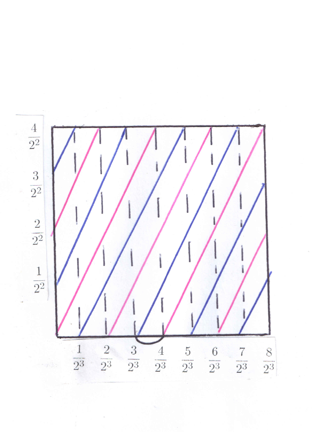
Figure 1. The case $n=2$

We assume now that $v=0,1,...,2^{n+1}-1$ is even.

In this case we consider the two terms of (6):

$${\color[rgb]{0,0,0}\sum_{j\,\,\text{such that}\,j+j_{0}=v\,\text{for some}\,j_{0}}\Pi_{w=0}^{n-1}J_{2}(\,T^{w}(\,\frac{j}{2^{n}}\,)\,)\int_{\frac{v-j}{2^{n}}}^{\frac{v-j+1}{2^{n}}}\,\tilde{J}_{n}(\frac{x}{2}\,+\,\frac{j}{2^{n+1}})\,f(\frac{x}{2}\,+\,\frac{j}{2^{n+1}})\,d\mu(x)\,}+\,$$ (7)

$${\color[rgb]{0,0,0}\sum_{j\,\,\text{such that}\,j+j_{0}=v-2^{n}\,\text{for some}\,j_{0}}\Pi_{w=0}^{n-1}J_{2}(T^{w}(\frac{j}{2^{n}}))\int_{\frac{v-j-2^{n}}{2^{n}}}^{\frac{v-j-2^{n}+1}{2^{n}}}\,\tilde{J}_{n}(\frac{x}{2}+\frac{j+2^{n}}{2^{n+1}})\,f(\frac{x}{2}+\frac{j+2^{n}}{2^{n+1}})\,d\mu(x)}=$$ (8)

$${\color[rgb]{0,0,0}\sum_{j\,\,\text{such that}\,j+j_{0}=v\,\text{for some}\,j_{0}}\Pi_{w=0}^{n-1}J_{2}(\,T^{w}(\,\frac{j}{2^{n}}\,)\,)\int_{\frac{v}{2^{n+1}}}^{\frac{v+1}{2^{n+1}}}\,\frac{\tilde{J}_{n}(u)}{J_{n}(u)}\,f(u)\,d\mu(u)\,}+\,$$ (9)

$${\color[rgb]{0,0,0}\sum_{j\,\,\text{such that}\,j+j_{0}=v-2^{n}\,\text{for some}\,j_{0}}\Pi_{w=0}^{n-1}J_{2}(\,T^{w}(\,\frac{j}{2^{n}}\,)\,)\int_{\frac{v}{2^{n+1}}}^{\frac{v+1}{2^{n+1}}}\,\frac{\tilde{J}_{n}(u)}{J_{n}(u)}\,f(u)\,d\mu(u)}=$$ (10)

$${\,\int_{\frac{v}{2^{n+1}}}^{\frac{v+1}{2^{n+1}}}\,\frac{\tilde{J}_{n}(u)}{J_{n}(u)}\,f(u)\,d\mu(u)}.$$ (11)

Assume that $v=0,1,...,2^{n+1}-1$ is even. In this case we consider the two terms of (5):

$$\sum_{0\leq t\leq 2^{n-1}-1\,}\,\Pi_{w=0}^{n-1}J_{2}(\,T^{w}(\,\frac{\frac{v-2t}{2}}{2^{n}}\,)\,)\,{\int_{\frac{2\,t}{2^{n}}}^{\frac{2\,t+1}{2^{n}}}J(x/2)f(x/2\,+\frac{\frac{v-2t}{2}}{2^{n}})d\mu(x)\,}+$$

$$\sum_{0\leq t\leq 2^{n-1}-1\,}\,\Pi_{w=0}^{n-1}J_{2}(\,T^{w}(\,\frac{\frac{v-2t}{2}-2^{n-1}}{2^{n}}\,)\,)\,{\int_{\frac{2\,t}{2^{n}}}^{\frac{2\,t+1}{2^{n}}}J(x/2\,+1/2)f(\,x/2\,+1/2\,+\,\frac{\frac{v-2t}{2}-2^{n-1}}{2^{n}})d\mu(x)}=$$

$$\sum_{j\,\,=1}^{2^{n-1}}\,\,\Pi_{w=0}^{n-1}J_{2}(\,T^{w}(\,\frac{j}{2^{n}}\,)\,)\,{\int_{\frac{v}{2^{n+1}}}^{\frac{v+1}{2^{n+1}}}\frac{J(u-\frac{j}{2^{n}})}{J_{n}(u)}f(u)\,d\mu(u)}.$$

Therefore, when $v$ even we get that for $u\in[\frac{v}{2^{n+1}},\frac{v+1}{2^{n+1}})$

$$\tilde{J}_{n}(u)=\sum_{j\,=1}^{2^{n-1}}\,\,\Pi_{w=0}^{n-1}J_{2}(\,T^{w}(\,\frac{j}{2^{n}}\,)\,)\,{\color[rgb]{0,0,0}J(u-\frac{j}{2^{n}})}$$

A similar result is true when $v$ is odd.

Remember that $\lim_{n\to\infty}\rho_{n}=\mu_{2}$.

As $J_{2}$ is a Hölder function, given any $x_{0}\in S^{1}$ we have that $\lim_{n\to\infty}\mathcal{L}^{n}_{\log J_{2}}(g)\,(x_{0})=\int g(z)d\mu_{2}(z)$. Then, we consider for $u\in S^{1}$ fixed, the function $x\to g(x)=J(u-x).$

Then, taking $x_{0}=0$ we get

$$\tilde{J}(u)=\lim_{n\to\infty}\,\tilde{J}_{n}(u)=\lim_{n\to\infty}\,\mathcal{L}^{n}_{\log J_{2}}(g)\,(0)=\int J(u-x)d\mu_{2}(x).$$

In this way

$$h(\nu)=-\int\log\tilde{J}(u)d\nu(u)=-\int\,\log\,(\,\int J(u-x)d\mu_{2}(x)\,)\,d\nu(x).$$

Remark 10.

Note also that if $J_{2}$ is continuous and satisfies the hypothesis of being the limit of $\rho_{n}$, $n\in\mathbb{N}$, the same expression $\tilde{J}(u)=\int J(u-x)d\mu_{2}(x)$ obtained above is also true.

In the case $J$ is constant $J=1/2$ we get that $\tilde{J}_{n}=1/2$. In this way if $\mu$ is the Lebesgue probability, then, $\nu_{n}=\mu*\rho_{n}$ is also Lebesgue probability.

Note that for any $u$ we have that $\tilde{J}_{n}(u)+\tilde{J}_{n}(u+1/2)=1$. In this way the probability $\nu_{n}$ is invariant for the $T$. Then, we get that the convolution of any invariant probability $\mu$ with $\rho_{n}$ (not invariant) is invariant.

The entropy of $\nu_{n}$ satisfies $h(\nu_{n})=-\int\log\tilde{J}_{n}d\nu(n)$.

3. Convolution of Gibbs probability and a periodic orbit of period two

In this section we consider the convolution of a Gibbs probability with a probability with support on an orbit of period two.

Suppose the Jacobian $J:S^{1}\to\mathbb{R}$ is such that $\mathcal{L}_{\log J}^{*}(\mu)=\mu$.

Consider now $\rho=\frac{1}{2}(\delta_{1/3}+\delta_{2/3})$ and we want to analyze properties of $\nu=\mu*\rho$.

We denote the Jacobian of $\nu$ (in the sense of Definition 1) by $\tilde{J}$. We have to understand in this case the corresponding change of coordinates on the inverse branches.

In other words, we want to express the $\tilde{J}$, such that,

$$\mathcal{L}_{\log\tilde{J}}^{*}\,(\nu)=\nu$$ (12)

in terms of $J$, $\rho$ and $\mu$.

We will present an explicit expression for $\tilde{J}$ in terms of $J$ and two more Radon-Nikodym derivatives (see expression (14)). This will provide a formula for the entropy of $\mu*\rho$ (see (17)).

We will also show that there exist Gibbs probabilities $\mu$ satisfying $\mu=\nu=\mu*\rho.$ Jacobians described by equation (21) satisfy this property. For these examples, of course, the entropy does not increase by convolution.

About question (12) the main property for $\tilde{J}$ is: for any continuous function $f$

$$\int\mathcal{L}_{\log\tilde{J}}(f)(z)d(\mu*\rho)(z)=\int f(z)d(\mu*\rho)(z).$$

In this way $\mu*\rho$ is a fixed point for $\mathcal{L}_{\log\tilde{J}}^{*}$.

Remember that when $\tilde{J}$ is Hölder the fixed point probability is unique.

For a continuous function $f$ we get

$$\int f(z)d(\mu*\rho)(z)=\int f(x+y)d\mu(x)\,d\rho(y)=$$

$$1/2\,(\int f(x+1/3)d\mu(x)\,+\,\int f(x+2/3)d\mu(x)\,)=$$

$$1/2\,(\int\mathcal{L}_{\log J}(f(x+1/3))d\mu(x)\,+\,\int\mathcal{L}_{\log J}(f(x+2/3))d\mu(x)\,)=$$

$$1/2\,(\,\int[J(x/2)(f(x/2\,+\,1/3))+J((x+1)/2)(f(\,(x+1)/2\,+\,1/3)\,)]d\mu(x)+$$

$$\int[J(x/2)(f(x/2\,+\,2/3))+J((x+1)/2)(f(\,(x+1)/2\,+\,2/3)\,)]d\mu(x)\,)=$$

$$1/2\,(\,\int[{J(x/2)\,f(x/2\,+\,1/3\,)}+{J((x+1)/2)\,f(\,x/2\,+\,5/6\,)}\,\,]\,d\mu(x)+$$

$$\int[{J(x/2)\,f(x/2\,+\,2/3\,)}+{J((x+1)/2)\,f(\,x/2\,+\,1/6\,)}\,]\,d\mu(x)\,).$$

On the other hand

$$\int\mathcal{L}_{\log\tilde{J}}(f)(z)d(\mu*\rho)(z)=$$

$$\int\mathcal{L}_{\log\tilde{J}}(f)(x+y)d\mu(x)\,d\rho(y)=$$

$$\int[\tilde{J}((x+y)/2)(f(\,(x+y)/2))+\tilde{J}((x+y+1)/2)(f(\,(x+y+1)/2\,)\,)]d\mu(x)\rho(y)\,=$$

$$1/2\,(\,\int[\,\tilde{J}((x+\,\,1/3)/2)\,f(\,(x+\,\,1/3)/2)\,+\tilde{J}(\,(x+\,\,1/3\,\,+1)/2)\,f(\,(x+\,\,1/3\,\,+1)/2\,)\,]d\mu(x)\,+$$

$$\int[\,\tilde{J}(\,(\,x\,+\,2/3\,)/2\,)\,f\,(\,(\,x\,+\,\,2/3\,\,)/2\,)+\tilde{J}(\,(\,x+\,2/3\,+1\,)/2\,)\,f(\,(\,x\,+\,\,2/3\,+\,1\,)/2\,)]\,d\mu(x)\,\,.$$

The above means that it is required that for any continuous $f$

$$\,\int[J(x/2)\,f(x/2\,+\,1/3\,)+J((x+1)/2)\,f(\,x/2\,+\,5/6\,)\,\,]\,d\mu(x)+$$

$$\int[J(x/2)\,f(x/2\,+\,2/3\,)+J((x+1)/2)\,f(\,x/2\,+\,1/6\,)\,]\,d\mu(x)\,=$$

$$\,\,\int[\,\tilde{J}(x/2\,+\,\,1/6\,)\,f(\,x/2+\,\,1/6)+\,\tilde{J}\,(x/2\,+\,\,2/3\,\,)\,f(\,x/2\,+\,\,2/3\,)\,]\,d\mu(x)\,+$$

$$\int[\,\tilde{J}(x/2+\,\,1/3\,)\,f\,(x/2+\,\,1/3\,)\,+\,\tilde{J}(x/2\,+\,5/6\,)\,f(\,x/2+\,\,5/6\,)\,]\,d\mu(x)\,.$$ (13)

3.1. An explicit expression for the convolution in the case of Gibbs probabilities for Hölder Jacobians

Consider a Hölder Jacobian $J$ on $S^{1}$ and suppose that $J$ is the Jacobian of $\mu$.

$\tilde{J}$ denotes the Jacobian of $\nu=\mu*\rho$.

We will not be able to show that $\tilde{J}$ is continuous (just measurable). Anyway, we denote $\tilde{J}$ as the Jacobian of $\nu$ in the sense of Remark 1.

In this subsection we want to show an explicit expression (in terms of certain Radon-Nidodym derivatives) for $\tilde{J}$ (see (14)). In order to get that we will have to use equation (13).

Denote by $\mu_{1}$ the probability such that $\mu_{1}(B)=\mu(B+1/3)$ for any Borel set $B$ and denote by $\mu_{2}$ the probability such that $\mu_{2}(B)=\mu(B+2/3)$ for any Borel set $B$.

The measure $\mu_{3}=\mu_{1}+\mu_{2}.$

Then, $\mu_{1}$ is absolutely continuous with respect to $\mu_{3}$. Denote by $R_{1}$ the Radon-Nikodym derivative.

Moreover, $\mu_{2}$ is absolutely continuous with respect to $\mu_{3}$. Denote by $R_{2}$ the corresponding Radon-Nykodim derivative.

Therefore, for any continuous function $h$ we have

$$\int hd\mu_{1}=\int h(z-1/3)d\mu(z)=\int h(z-1/3)R_{1}(z-1/3)d\mu(z)+\int h(z-2/3)R_{1}(z-2/3)d\mu(z)$$

and

$$\int hd\mu_{2}=\int h(z-2/3)d\mu(z)=\int h(z-1/3)R_{2}(z-1/3)d\mu+\int h(z-2/3)R_{2}(z-2/3)d\mu(z).$$

Taking above $h(z)=g(z+1/3)$ the first condition can be rewritten as: for any continuous function $g$:

$$\int gd\mu=\int g(z)R_{1}(z-1/3)d\mu(z)+\int g(z-1/3)R_{1}(z-2/3)d\mu(z).$$

Taking above $h(z)=g(z+2/3)$ the first condition can be rewritten as: for any continuous function $g$:

$$\int gd\mu=\int g(z+1/3)R_{2}(z-1/3)d\mu(z)+\int g(z)R_{2}(z-2/3)d\mu(z)$$

We will show that

$$\tilde{J}(z)=J(z-2/6)R_{1}(2z)+J(z-4/6)R_{2}(2z).$$ (14)

This corresponds also to

$$\tilde{J}(x/2+5/6)=J(x/2+3/6)R_{1}(x-1/3)+J(x/2+1/6)R_{2}(x/2-1/3)$$ (15)

and

$$\tilde{J}(x/2+2/3)=J(x/2+2/6)R_{1}(x-2/3)+J(x/2)R_{2}(x/2-2/3).$$ (16)

It will follow that the entropy of $\nu$ is

$$h(\nu)=-\int\log(\,\,J(z-2/6)R_{1}(2z)+J(z-4/6)R_{2}(2z)\,\,)\,d\nu.$$ (17)

Remark 11.

Note that for any $x$ we have that $R_{1}(x)+R_{2}(x)=1$. The above expression for $\tilde{J}$ in (14) says in some sense that $\tilde{J}$ attain values on the convex hull of the values of $J$. It is reasonable to guess that this mechanism is responsible for the increase of entropy under convolution (see a kind of more general and analytic statement in the appendix). Expression (17) permits an analytic estimation of this increase.

Assuming (14) we have to show that (13) is true for any $f$.

a) Consider first a function $f$ with support on $(0,1/6).$

We have to show that

$$\int_{2/3}^{1}{J(x/2)\,f(x/2\,+\,2/3\,)}\,\ d\mu(x)+\int_{1/3}^{2/3}{J(x/2\,+\,1/2)\,f(\,x/2\,+\,5/6\,)}\,\,d\mu(x)\,=$$

$$\int_{2/3}^{1}\,{\tilde{J}\,(x/2\,+\,\,2/3\,\,)\,f(\,x/2\,+\,\,2/3\,)}\,d\mu(x)\,+\,\int_{1/3}^{2/3}{\tilde{J}(x/2\,+\,5/6\,)\,f(\,x/2+\,\,5/6\,)}\,d\mu(x)\,\,.$$ (18)

From (14), (15) and (16) we get

$$\int_{2/3}^{1}J(x/2)\,f(x/2\,+\,2/3\,)\,\ d\mu(x)+\int_{1/3}^{2/3}J(x/2\,+\,1/2)\,f(\,x/2\,+\,5/6\,)\,\,d\mu(x)\,=$$

$$[\,\int_{2/3}^{1}J(x/2)\,f(x/2\,+\,2/3\,)\,R_{2}(x-2/3)\ d\mu(x)+\int_{1/3}^{2/3}J(x/2+1/6)\,f(x/2\,+\,5/6\,)\,R_{2}(x-1/3)\ d\mu(x)\,]\,+$$

$$[\int_{2/3}^{1}J(x/2+2/6)f(x/2+2/3)R_{1}(x-2/3)d\mu(x)+\int_{1/3}^{2/3}J(x/2+3/6)f(x/2+\,5/6)R_{1}(x-1/3)d\mu(x)]=$$

$$[\,\,\int_{2/3}^{1}J(x/2)f(x/2+2/3)R_{2}(x-2/3)d\mu(x)+\int_{2/3}^{1}J(x/2+2/6)f(x/2+2/3)R_{1}(x-2/3)d\mu(x)\,\,]+$$

$$[\,\int_{1/3}^{2/3}J(x/2+3/6)f(x/2+\,5/6)R_{1}(x-1/3)d\mu(x)+\int_{1/3}^{2/3}J(x/2+1/6)\,f(x/2\,+\,5/6\,)\,R_{2}(x-1/3)\ d\mu(x)\,]=$$

$$[\,\,\int_{2/3}^{1}f(x/2+2/3)\,\,(\,J(x/2)R_{2}(x-2/3)d\mu(x)+J(x/2+2/6)R_{1}(x-2/3)\,)\,\,d\mu(x)\,\,]+$$

$$[\,\int_{1/3}^{2/3}f(x/2+\,5/6)\,\,\,(\,J(x/2+3/6)R_{1}(x-1/3)d\mu(x)+\ J(x/2+1/6)\,\,R_{2}(x-1/3)\,)d\mu(x)\,]=$$

$$\int_{2/3}^{1}f(x/2+2/3)\,\,\tilde{J}(x/2+2/3)\,\,d\mu(x)\,\,+\,\int_{1/3}^{2/3}f(x/2+\,5/6)\,\,\tilde{J}(x/2+5/6)d\mu(x)\,,$$

and this shows (18).

b) Suppose $f$ has support on the interval $[2/6,3/6).$

We have to show that

$$\int_{0}^{1/3}{J(x/2)\,f(x/2\,+\,1/3\,)}\,\ d\mu(x)+\int_{1/3}^{2/3}{J(y/2+1/2)\,f(\,y/2\,+\,1/6\,)}\,\,d\mu(y)\,=$$

$$\int_{0}^{1/3}\,{\tilde{J}\,(x/2\,+\,\,1/3\,\,)\,f(\,x/2\,+\,\,1/3\,)}\,d\mu(x)\,+\,\int_{1/3}^{2/3}{\tilde{J}(y/2+\,\,1/6)\,f(\,y/2+\,\,1/6\,)}\,d\mu(y)\,\,.$$ (19)

The proof is similar to the previous case and it will be left for the reader.

c) Suppose the function $f$ has support on $(4/6,5/6).$ We have to show that

$$\int_{0}^{1/3}{J(x/2)\,f(x/2\,+\,2/3\,)}\,\ d\mu(x)+\int_{2/3}^{1}{J(y/2)\,f(\,y/2\,+\,1/3\,)}\,\,d\mu(y)\,=$$

$$\int_{0}^{1/3}\,{\tilde{J}\,(x/2\,+\,\,2/3\,\,)\,f(\,x/2\,+\,\,2/3\,)}\,d\mu(x)\,+\,\int_{2/3}^{1}{\tilde{J}(y/2\,+\,1/3\,)\,f(\,y/2+\,\,1/3\,)}\,d\mu(y)\,\,.$$ (20)

The proof is similar to the previous case and it will be left for the reader.

For functions $f$ with support on the other possible intervals we proceed in a similar way. This will give the explicit expression of $\tilde{J}$ in terms of $J,R_{1},R_{2}$ on all points.

3.2. A class of examples where $J=\tilde{J}$

Suppose we ask: when $J=\tilde{J}$? What equation should $J$ satisfy in this case? Is there some special form of $J$ such that this happens? We will present examples where this happens.

Denote by $\mathcal{S}$ the class of positive Hölder Jacobians $J$ such that for any $x\in[0,1/6)$ we have

$$J(x)=J(x-2/6)=J(x-4/6).$$ (21)

We point out that under the above conditions the values of $J$ on $[0,1/6)$ determine $J$ uniquely. Indeed, on the intervals $[0,1/6)$ $[2/6,3/6)$ and $[4/6,5/6]$ is clearly determined. On the intervals of the form $[1/6,2/6)$ $[3/6,4/6)$ and $[5/6,1)$ it is also determined because the sum of $J$ on the preimages of any point is equal to $1$.

There exist several continuous (and Hölder) Jacobians satisfying such conditions.

The equation

$$J(z)=J(z-2/6)R_{1}(2z)+J(z-4/6)R_{2}(2z)$$

is true for any $f\in\mathcal{S}$ and any $z\in S^{1}$ because $R_{1}+R_{2}=1$.

As from (14) we get that for any $z$

$$\tilde{J}(z)=J(z-2/6)R_{1}(2z)+J(z-4/6)R_{2}(2z),$$

it follows that in this case $\tilde{J}=J$ and $\mu=\mu*\rho.$

4. Differentiability of the entropy of convolution

To each equilibrium probability for a Hölder potential $A$ one can associate a unique positive Holder Jacobian. Therefore, the set of equilibrium probabilities can be considered as a Banach manifold $\mathcal{N}$ (see [3]). In this way we can consider the bijective map $\log J\to\mu_{\log J}$ over $\mathcal{N}$.

Given a probability $\mu_{\log J}\in\mathcal{N}$ (associated to the potential $\log J$) and a tangent vector $\zeta\in T_{\mu_{\log J}}\mathcal{N}$, one is interested on the derivative $\mu_{\log+\zeta}$ along $\zeta$, where $\mu_{\log J+\zeta}$ is the equilibrium probability for the potential $\log J+\zeta.$

For a fixed $\varphi$ consider the transformation $G_{\varphi}$, such that, $G_{\varphi}(\log J)=\int\varphi\,d\mu_{\log J}$, then,

$$D(G_{\varphi})_{\log J}(\zeta)=\int(I-\mathcal{L}_{\log J})^{-1}(\varphi)\cdot\zeta\,d\mu_{\log J}=$$

$$\sum_{i=0}^{+\infty}\int\varphi\cdot\zeta\circ T^{i}\,d\mu_{\log J}.$$

Given a Hölder potential $A$, following [3], denote $\mathcal{N}(A)=\log J$, where $J$ is the Jacobian of the equilibrium probability for $A$. We also denote $\mu_{\mathcal{N}(A)}$ the Gibbs (equilibrium) probability for $A$.

We denote $\mu_{i}$, $i=1,2$, the probability associated, respectively, to the Jacobians $(\log J)_{i}.$

We denote $\mu^{t}=\mu_{\mathcal{N}(\log J_{1}+tz_{3})}$, where $z_{3}$ is a tangent vector to the manifold of Gibbs probabilities at the point $\mu_{1}$. Note that in this case $\int z_{3}\,\,d\mu_{1}=0$.

Denote by $J_{1}^{t}$ the Jacobian of $\mu^{t}$. This means that $\log J_{1}^{t}=\mathcal{N}(\log J_{1}+tz_{3}).$

If $\nu_{t}=\mu^{t}*\mu_{2}$ we get that

$$h(\nu_{t})=-\int\,[\,\,\int\,\log\,(\,\int J_{1}^{t}(r+s-x)d\mu_{2}(x)\,)\,d\mu_{2}(r)\,\,]\,\,d\mu^{t}(s)$$

Denote

$$Z^{t}(s)=\int\,\log\,(\,\int J_{1}^{t}(r+s-x)d\mu_{2}(x)\,)\,d\mu_{2}(r)\,\,.$$

Then,

$$\frac{d}{dt}h(\nu_{t})|_{t=0}=-\int\frac{d}{dt}|_{t=0}\,\,Z^{t}(s)\,d\nu_{t}|_{t=0}(s)-\int Z^{t}(s)\,\,|_{t=0}\,\,\frac{d}{dt}|_{t=0}d\nu_{t}(s).$$

Given a continuous function $\phi$ we have from [3] that

$$\int\phi(s)\,\,\,\,\frac{d}{dt}|_{t=0}d\nu_{t}(s)=\int\phi\,z_{3}\,d\mu_{1}.$$

Note that $Z^{t}-Z^{0}$ goes uniformly to zero when $t\to 0.$

Therefore, from [3]

$$\int Z^{t}(s)\,\,|_{t=0}\,\,\frac{d}{dt}|_{t=0}d\nu_{t}(s)=$$

$$\int Z^{0}(s)\,\,\,\,\frac{d}{dt}|_{t=0}d\nu_{t}(s)=$$

$$\int\,\,[\int\,\log\,(\,\int J_{1}(r+s-x)d\mu_{2}(x)\,)\,d\mu_{2}(r)]\,\,\frac{d}{dt}|_{t=0}d\nu_{t}(s)=$$

$$\int\,\,[\int\,\log\,(\,\int J_{1}(r+s-x)d\mu_{2}(x)\,)\,d\mu_{2}(r)]\,\,z_{3}(s)d\mu_{1}(s).$$

We denote by $\varphi^{t}$ and $\lambda^{t}$, respectively, the main eigenfunction and the main eigenvalue of the Ruelle operator for the potential $\log(J_{1})+tz_{3}.$

Note that when $t=0$ we get that $\varphi^{t}=1$ and $\lambda^{t}=1$.

As

$$\log(J_{1}^{t})=\log(J_{1})+\,t\,z_{3}\,+\log\varphi_{t}-\log(\varphi_{t}\circ T)-\log\lambda^{t},$$

which means

$$J_{1}^{t}=J_{1}\,e^{t\,z_{3}+\log\varphi_{t}-\log(\varphi_{t}\circ T)-\log\lambda^{t}},$$

we get that

$$Z^{t}(s)=\int\,\log\,(\,\int J_{1}\,e^{t\,z_{3}+\log\varphi_{t}-\log(\varphi_{t}\circ T)-\log\lambda^{t}}(r+s-x)d\mu_{2}(x)\,)\,d\mu_{2}(r)\,\,.$$

and

$$\frac{d}{dt}|_{t=0}\,\,Z^{t}(s)=$$

$$\int\,\frac{d}{dt}|_{t=0}\,\,[\,\,\log\,(\,\int J_{1}\,e^{t\,z_{3}+\log\varphi_{t}-\log(\varphi_{t}\circ T)-\log\lambda^{t}}(r+s-x)\,\,\,\,d\mu_{2}(x)\,]\,d\mu_{2}(r)\,\,.$$

Denote

$$Y^{t}(s,r)=\,\,\,(\,\int J_{1}\,(r+s-x)e^{t\,z_{3}+\log\varphi_{t}-\log(\varphi_{t}\circ T)-\log\lambda^{t}}(r+s-x)\,\,d\mu_{2}(x).$$

Therefore,

$$-\int\frac{d}{dt}|_{t=0}\,\,Z^{t}(s)\,d\nu_{t}|_{t=0}(s)=-\int\frac{\frac{d}{dt}|_{t=0}\,\,Y^{t}(s,r)}{Y^{0}(s,r)}\,d\mu_{2}(r)\,d\mu_{1}(s).$$

Now we estimate

$$\frac{d}{dt}|_{t=0}\,\,Y^{t}(s,r)=$$

$$\int J_{1}\,\,(r+s-x)\,[\,z_{3}+\frac{d}{dt}|_{t=0}\,(\,\log\varphi_{t}-\log(\varphi_{t}\circ T)-\log\lambda^{t}\,)(r+s-x)\,]\,d\mu_{2}(x).$$

Finally,

$$-\int\frac{d}{dt}|_{t=0}\,\,Z^{t}(s)\,d\nu_{t}|_{t=0}(s)=$$

$$-\int\frac{\int J_{1}\,\,(r+s-x)\,[\,z_{3}+\frac{d}{dt}|_{t=0}\,(\,\log\varphi_{t}-\log(\varphi_{t}\circ T)-\log\lambda^{t}\,)\,](r+s-x)\,d\mu_{2}(x)}{\int J_{1}\,\,(r+s-x)\,d\mu_{2}(x)}\,d\mu_{2}(r)\,d\mu_{1}(s)$$

In this way we get the following proposition:

Proposition 12.

Suppose $\mu_{i}$, $i=1,2$ are probabilities associated, respectively, to the Jacobians $\log J_{i}.$

Denote $\mu^{t}=\mu_{\mathcal{N}(\log J_{1}+tz_{3})}$, $t\in\mathbb{R}$ small, where $z_{3}$ is a tangent vector to the manifold of Gibbs probabilities at the point $\mu_{1}$, and $\nu_{t}=\mu^{t}*\mu_{2}$.

We also denote by $\varphi^{t}$ and $\lambda^{t}$, respectively, the main eigenfunction and the main eigenvalue of the Ruelle operator for the potential $\log(J_{1})+tz_{3}.$

Then,

$$\frac{d}{dt}h(\nu_{t})|_{t=0}=$$

$$-\int\frac{\int J_{1}\,\,(r+s-x)\,[\,z_{3}+\frac{d}{dt}|_{t=0}\,(\,\log\varphi_{t}-\log(\varphi_{t}\circ T)-\log\lambda^{t}\,)\,](r+s-x)\,d\mu_{2}(x)}{\int J_{1}\,\,(r+s-x)\,d\mu_{2}(x)}\,d\mu_{2}(r)\,d\mu_{1}(s)$$

$$-\,\int\,\,[\int\,\log\,(\,\int J_{1}(r+s-x)d\mu_{2}(x)\,)\,d\mu_{2}(r)]\,\,z_{3}(s)d\mu_{1}(s).$$

5. Appendix

Now we will prove a result inspired by the reasoning followed in section 3 (see Remark 11).

It a result of interest in itself.

Proposition 13.

Suppose are given the Hölder Jacobians $J_{1}$ and $J_{2}$ and they are such that: $J_{2}\geq J_{1}$ when $J_{1}\geq 1/2$, and $J_{2}\leq J_{1}$ when $J_{1}\leq 1/2$.

Denote $\mu_{i}$ the Gibbs probability associated to the Hölder potential $\log J_{i}$, $i=1,2$. Then, $h(\mu_{1})\geq h(\mu_{2})$.

Proof:

One way to get a path from $J_{1}$ to $J_{2}$ is to take $J^{\,t}=J_{1}+t\,(J_{2}-J_{1}),$ $t\in[0,1]$.

Note that $J^{\,t}(x_{1})+J^{t}(x_{2})=1$, if $T(x_{1})=T(x_{2})$ (therefore $J^{\,t}$ is a Hölder Jacobian for each value $t$).

We know that if $\int\,\chi\,d\mu_{1}=0$, then, the entropy $h_{t}$ of the Gibbs state associated to $\log J_{1}+\,t\,\chi$ satisfies

$$\frac{d\,h_{t}}{dt}_{t=0}=-\int\,\chi\,\log J_{1}\,d\mu_{1}=-\int\,\chi\,(\log J_{1}-\log 1/2)\,d\mu_{1}$$

(see page 38 in [3]).

In this way if $\chi(x)\geq 0$ when $(\log J_{1}(x)-\log 1/2)\geq 0$ and $\chi(x)\leq 0$ when $(\log J_{1}(x)-\log 1/2)\leq 0$ we get that the entropy decreases when we go in the direction $\chi$ beginning on $\mu_{1}$. This is so because $-\int\,\chi\,\log J_{1}\,\,d\mu_{1}<0$.

Take $\epsilon(t)$ such that

$$\log J_{1}+\epsilon(t)=\log(\,J_{1}+t\,(J_{2}-J_{1})\,).$$

Note that $\log J_{1}+\epsilon(1)=\log(\,J_{2})$.

Then, $\frac{d}{dt}\epsilon(t)|_{t=0}=\frac{J_{2}}{J_{1}}-1$.

Moreover,

$$\int\,(\frac{J_{2}}{J_{1}}-1)\,d\mu_{1}=\int\,\frac{J_{2}}{J_{1}}\,d\mu_{1}-1=$$

$$\int\,\mathcal{L}_{\log J_{1}}\,(\frac{J_{2}}{J_{1}}\,)\,d\mu_{1}-1=\int\,\mathcal{L}_{\log J_{2}}\,(1)d\mu_{1}\,-1=0$$

The proof that $\frac{d}{dt}\epsilon(t)|_{t=0}\leq 0$ is similar to the case $t=0.$

We denote $\mu^{t}$ the equilibrium state for the normalized potential $\log(J_{1})+\epsilon(t).$

Moreover, $\frac{d}{dt}\epsilon(t)|_{t}=\frac{J_{2}-J_{1}}{J_{1}\,-t\,(J_{2}-J_{1})}$.

In this case

$$\int\frac{d}{dt}\epsilon(t)|_{t}\,d\mu^{t}=\int\frac{J_{2}-J_{1}}{J_{1}\,+t\,(J_{2}-J_{1})}d\mu^{t}=$$

$$\int\mathcal{L}_{\log(J_{1}\,+t\,(J_{2}-J_{1}))}\,(\,\frac{J_{2}-J_{1}}{J_{1}\,+t\,(J_{2}-J_{1})}\,)d\mu^{t}=$$

$$\int\mathcal{L}_{0}(J_{1}-J_{2})d\mu^{t}=0.$$

Then, $\frac{d}{dt}\epsilon(t)|_{t}=\chi_{\,t}$, $t\in[0,1]$ is tangent vector on $\mathcal{N}$ at $\log J_{\,t}$.

Moreover,

$$\frac{d\,h_{t}}{dt}|_{t}=-\int\,\chi_{\,t}\,\log J_{t}\,d\mu_{t}=-\int\,\chi_{\,t}\,(\log J_{t}-\log 1/2)\,d\mu_{t}=$$

$$-\int\,\frac{J_{2}-J_{1}}{J_{1}\,+t\,(J_{2}-J_{1})}\,(\log(\,J_{1}+t(J_{2}-J_{1})\,)-\log 1/2)\,d\mu_{t}.$$

Remember that $J_{2}\geq J_{1}$ when $J_{1}\geq 1/2$, and $J_{2}\leq J_{1}$ when $J_{1}\leq 1/2$.

When, $J_{2}-J_{1}\geq 0,$ we get that $(\log(\,J_{1}+t(J_{2}-J_{1})\,)-\log 1/2)\geq 0.$

On the other hand when $J_{2}-J_{1}\leq 0,$ we get that $(\log(\,J_{1}+t(J_{2}-J_{1})\,)-\log 1/2)\leq 0.$

Therefore, $\frac{d\,h_{t}}{dt}|_{t}\leq 0.$

∎

References

- [1] L. Barchinski, -convolução e o operador de transferência generalizado, PhD. thesis, Pos-Grad Mat - UFRGS (2016)
- [2] M. Bramson and S. Kalikow, Nonuniqueness in g-functions. Israel J. Math. 84, no. 1-2, 153–160 (1993)
- [3] P. Giulietti, B. Kloeckner, A. O. Lopes and D. Maicon, The calculus of Thermodynamical Formalism, to appear in JEMS
- [4] M. Hochman and P. Shmerkin, Local entropy averages and projections of fractal measures, Annals of Mathematics, Vol. 175, No. 3, 1001–1059 (May, 2012)
- [5] B. Kloeckner, A. O. Lopes and M. Stadlbauer, Contraction in the Wasserstein metric for some Markov chains, and applications to the dynamics of expanding maps, Nonlinearity, 28, Number 11, 4117–4137 (2015)
- [6] E. Lindenstrauss, D. Meiri and Y. Peres, Entropy of Convolutions on the Circle, Annals of Mathematics, Vol. 149, No. 3, 871-904 (1999)
- [7] A. O. Lopes, An analogy of charge distribution on Julia sets with the Brownian motion. J. Math. Phys. 30 9, 2120-2124 (1989)
- [8] A. O. Lopes, J. K. Mengue, J. Mohr and R. R. Souza, Entropy and Variational Principle for one-dimensional Lattice Systems with a general a-priori probability: positive and zero temperature, Erg. Theory and Dyn Systems, 35 (6), 1925–1961 (2015)
- [9] A. O. Lopes, Entropy and Large Deviation, NonLinearity, Vol. 3, N. 2, 527-546 (1990).
- [10] D. Meiri, Entropy and uniform distribution of orbits in , Israel J. Math. 105, 155–183 (1998)
- [11] D. Meiri, Entropy, dimension and distribution of orbits in , Ph.D. thesis, Hebrew University, Jerusalem (1981)
- [12] D. Meiri and Y. Peres, Bi-invariant sets and measures have integer Hausdorff dimension, Ergodic Theory and Dynamical Systems 19, 523–534 (1999)
- [13] E. Mihailescu and M. Urbanski, Measure-theoretic degrees and topological pressure for nonexpanding transformations, J. Functional Analysis, 267, no. 8, 2823–2845 (2014).
- [14] W. Parry and M. Pollicott, Zeta functions and the periodic orbit structure of hyperbolic dynamics, Astérisque 187–188 268 pp (1990).
- [15] W. Parry, Entropy and generators in ergodic theory, W.A. Benjamin, Inc. (1969).
- [16] F. Przytycki and M. Urbanski, Conformal Fractals: Ergodic Theory Methods, London Math, Soc. (2010)
- [17] A. Quas, Non-ergodicity for expanding maps and g-measures. Ergodic Theory Dynam. Systems 16 , no. 3, 531–543 (1996)
- [18] V. Ramos and M. Viana, Equilibrium states for hyperbolic potentials, Nonlinearity 30, 825-847 (2017)
- [19] D. Ruelle, Thermodynamic formalism. The mathematical structures of equilibrium statistical mechanics, Cambridge Univ. Press (2004).
- [20] B. B. Uggioni, Convergencia da convolução de probabilidades invariantes pelo deslocamento, PhD thesis, Pos-Grad - Mat UFRGS (2016).
- [21] M. Viana and K. Oliveira, Foundations of Ergodic Theory, Cambridge Press (2016)