Decentralized 2-D Control of Vehicular Platoons
under Limited Visual Feedback

Abstract

In this paper, we consider the two dimensional (2-D) predecessor-following control problem for a platoon of unicycle vehicles moving on a planar surface. More specifically, we design a decentralized kinematic control protocol, in the sense that each vehicle calculates its own control signal based solely on local information regarding its preceding vehicle, by its on-board camera, without incorporating any velocity measurements. Additionally, the transient and steady state response is a priori determined by certain designer-specified performance functions and is fully decoupled by the number of vehicles composing the platoon and the control gains selection. Moreover, collisions between successive vehicles as well as connectivity breaks, owing to the limited field of view of cameras, are provably avoided. Finally, an extensive simulation study is carried out in the WEBOTS${}^{\text{TM}}$ realistic simulator, clarifying the proposed control scheme and verifying its effectiveness.

I Introduction

During the last few decades, the 1-D longitudinal control problem of Automated Highway Systems (AHS) has become an active research area in automatic control (see [1, 2, 3, 4, 5] and the references therein). Unlike human drivers that are not able to react quickly and accurately enough to follow each other in close proximity at high speeds, the safety and capacity of highways (measured in vehicles/lanes/time) is significantly increased when vehicles operate autonomously, forming large platoons at close spacing. However, realistic situations necessitate for 2-D motion on planar surfaces (see Fig. 1).

Early works in [6, 7, 8, 9] consider the lane-keeping and lane-changing control for platoons in AHS, adopting however a centralized network, where all vehicles exchange information with a central computer that determines the control protocol, making thus the overall system sensitive to delays, especially when a large number of vehicles is involved. Alternatively, rigid multi-agent formations are employed in decentralized control schemes, where each vehicle utilizes relative information from its neighbors. The majority of these works consider unicycle [10, 11, 12, 13, 14] and bicycle kinematic models [15, 16, 17]. However, many of them adopt linearization techniques [11, 18, 19, 13, 20, 15, 17, 21] that may lead to unstable inner dynamics or degenerate configurations owing to the non-holonomic constraints of the vehicles, as shown in [22]. Additionally, each vehicle is assumed to have access to the neighboring vehicles’ velocity, either explicitly, hence degenerating the decentralized form of the system and imposing inherent communication delays, or by employing observers [14] that increase the overall design complexity. Furthermore, the transient and steady state response of the closed loop is affected severely by the control gains selection [23], thus limiting the controller’s robustness and complicating the design procedure.

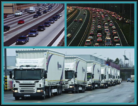
Figure 1: Vehicular platoons in 2-D motion on planar roads.

Another significant issue affecting the $2$-D control of vehicular platoons concerns the sensing capabilities when visual feedback from cameras is employed. A vast number of the related works neglects the sensory limitations, which however are crucial in real-time scenarios. In [13, 22] visual feedback from omnidirectional cameras is adopted, not accounting thus for sensor limitations, which however are examined in [10] considering directional sensors for the tracking problem of a moving object by a group of robots. Although cameras are directional sensors, they inherently have a limited range and a limited angle of view as well. Hence, in such cases each agent should keep a certain close distance and heading angle from its neighbors, in order to avoid connectivity breaks. Thus, it is clear that limited sensory capabilities lead to additional constraints on the behavior of the system, that should therefore be taken into account exclusively when designing the control protocols. The aforementioned specifications were considered in [24], where a solution based on set-theory and dipolar vector fields was introduced. Alternatively, a visual-servoing scheme for leader-follower formation was presented in [25]. Finally, a centralized control protocol under vision-based localization for leader-follower formations was adopted in [26, 27].

In this paper, we extend our previous work on 1-D longitudinal control of vehicular platoons [28] to $2$-D motion on planar surfaces, under the predecessor-following architecture. We design a fully decentralized kinematic control protocol, in the sense that each vehicle has access only to the relative distance and heading error with respect to its preceding vehicle. Such information is obtained by an onboard camera with limited field of view [12], that imposes inevitably certain constraints on the configuration of the platoon. More specifically, each vehicle aims at achieving a desired distance from its predecessor, while keeping it within the field of view of its onboard camera in order to maintain visual connectivity and avoid collisions. Moreover, the transient and steady state response is fully decoupled by the number of vehicles and the control gains selection. Finally, the explicit collision avoidance and connectivity maintenance properties are imposed by certain designer-specified performance functions, that incorporate the aforementioned visual constraints. In summary, the main contributions of this work are given as follows:

• We propose a novel solution to the $2$-D formation control problem of vehicular platoons, avoiding collisions and connectivity breaks owing to visual feedback constraints.

• We develop a fully decentralized kinematic control protocol, in the sense that the feedback of each vehicle is based exclusively on its own camera, without incorporating any measurement of the velocity of the preceding vehicle.

• The transient and steady state response of the closed loop system is explicitly determined by certain designer-specified performance functions, simplifying thus the control gains selection.

The manuscript is organized as follows. The problem statement is given in Section II. The decentralized control protocol is provided in Section III. In Section IV, an extensive simulation study is presented, clarifying and verifying the theoretical findings. Finally, we conclude in Section V.

II Problem Statement

Consider a platoon of $N$ vehicles moving on a planar surface under unicycle kinematics:

$$\left.\begin{array}[c]{l}\dot{x}_{i}=v_{i}\cos\varphi_{i}\\ \dot{y}_{i}=v_{i}\sin\varphi_{i}\\ \dot{\varphi}_{i}=\omega_{i}\end{array}\right\}\text{, }i=1,\dots,N$$ (1)

where $x_{i}$, $y_{i}$, $\varphi_{i}$ denote the position and orientation of each vehicle on the plane and $v_{i},\omega_{i}$ are the linear and angular velocities respectively. Let us also denote by $d_{i}(t)$ and $\beta_{i}(t)$ the distance and the bearing angle between successive vehicles $i$ and $i-1$ (see Fig. 2). Furthermore, we assume that the only available feedback concerns the distance $d_{i}(t)$ and the bearing angle $\beta_{i}(t)$, which both emanate from an onboard camera that detects a specific marker on the preceding vehicle (e.g., the number plate). The control objective is to design a distributed control protocol based exclusively on visual feedback such that $d_{i}(t)\rightarrow d_{i,des}$ and $\beta_{i}(t)\rightarrow 0$, i.e., each vehicle tracks its predecessor and maintains a prespecified desired distance $d_{i,des}$. Additionally, $d_{i}(t)$ should be kept greater than $d_{\mathsf{col}}$ to avoid collisions between successive vehicles. In the same vein, the inter-vehicular distance $d_{i}(t)$ and the bearing angle $\beta_{i}(t)$ should be kept less than $d_{\mathsf{con}}>d_{\mathsf{col}}$ and $\beta_{\mathsf{con}}$ respectively, in order to maintain the connectivity owing to the camera’s limited field of view (see Fig. 2). Moreover, the desired trajectory of the formation is generated by a reference/leading unicycle vehicle:

$$\begin{array}[c]{l}\dot{x}_{0}=v_{0}\cos\varphi_{0}\\ \dot{y}_{0}=v_{0}\sin\varphi_{0}\\ \dot{\varphi}_{0}=\omega_{0}\end{array}$$

with bounded velocities $v_{0}(t)$, $\omega_{0}(t)$ and is only provided to the first vehicle. Finally, to solve the aforementioned control problem, we assume that initially each vehicle lies within the field of view of its follower’s camera and no collision occurs, which are formulated as follows.

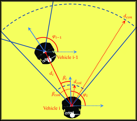
Figure 2: Graphical illustration of two successive vehicles in the platoon. Each vehicle should keep its distance $d_{i}\left(t\right)$ and bearing angle $\beta_{i}\left(t\right)$ to its predecessor within the feasible area $d_{\mathsf{col}}<d_{i}\left(t\right)<d_{\mathsf{con}}$ and $\left|\beta_{i}\left(t\right)\right|<\beta_{\mathsf{con}}$, thus avoiding collisions and connectivity breaks.

Assumption A1. The initial state of the platoon does not violate the collision and connectivity constraints, i.e., $d_{\mathsf{col}}<d_{i}(0)<d_{\mathsf{con}\text{ }}$ and $\left|\beta_{i}(0)\right|<\beta_{\mathsf{con}}$, $i=1,\dots,N$.

In the sequel, we define the distance and heading errors:

$$\left.\begin{array}[c]{l}e_{d_{i}}(t)=d_{i}(t)-d_{i,des}\\ e_{\beta_{i}}(t)=\beta_{i}(t)\end{array}\right\}\text{, }i=1,\dots,N$$ (2)

where $d_{i}\left(t\right)=\sqrt{\left(x_{i}\left(t\right)-x_{i-1}\left(t\right)\right){}^{2}+\left(y_{i}\left(t\right)-y_{i-1}\left(t\right)\right){}^{2}}$. Hence, differentiating (2) with respect to time and substituting (1), we obtain:

$$\left.\begin{array}[c]{l}\dot{e}_{d_{i}}=-v_{i}\cos\beta_{i}+v_{i-1}\cos(\gamma_{i}+\beta_{i})\\ \dot{e}_{\beta_{i}}=-\omega_{i}+\frac{v_{i}}{d_{i}}\sin\beta_{i}-\frac{v_{i-1}}{d_{i}}\sin(\gamma_{i}+\beta_{i})\end{array}\right\}\text{, }i=1,\dots,N$$ (3)

where $\gamma_{i}(t)=\varphi_{i}(t)-\varphi_{i-1}(t)$, which may be expressed in vector form as follows:

$$\begin{array}[c]{l}\dot{e}_{d}=-\tilde{C}v+c\\ \dot{e}_{\beta}=-\omega+D^{-1}(\tilde{S}v+s)\end{array}$$ (4)

where

$$e_{d} =\left[e_{d_{1}},\dots,e_{d_{N}}\right]^{T}\text{, }e_{\beta}=\left[e_{\beta_{1}},\dots,e_{\beta_{N}}\right]^{T}$$

$$v =[v_{1},\dots,v_{N}]^{T}\text{, }\omega=[\omega_{1},\dots,\omega_{N}]^{T}$$

$$D =\mathrm{diag}(d_{1},\dots,d_{N})^{T}$$

$$c =[v_{0}\cos(\gamma_{1}+\beta_{1}),0,\dots,0]^{T}$$

$$s =[v_{0}\sin(\gamma_{1}+\beta_{1}),0,\dots,0]^{T}$$

and $\tilde{C}$, $\tilde{S}$ are the lower bi-diagonal matrices:

$$\begin{array}[c]{l}{\tilde{C}}{=}\left[\begin{array}[c]{cccc}\cos\beta_{1}&0&\cdots&0\\ -\cos(\beta_{2}+\gamma_{2})&\cos\beta_{2}&&\vdots\\ 0&\ddots&\ddots&\\ &&\ddots&0\\ 0&\cdots&-\cos(\beta_{N}+\gamma_{N})&\cos\beta_{N}\end{array}\right]\\ \\ {\tilde{S}}{=}\left[\begin{array}[c]{cccc}\sin\beta_{1}&0&\cdots&0\\ -\sin(\beta_{2}+\gamma_{2})&\sin\beta_{2}&&\vdots\\ 0&\ddots&\ddots&\\ &&\ddots&0\\ 0&\cdots&-\sin(\beta_{N}+\gamma_{N})&\sin\beta_{N}\end{array}\right].\end{array}$$

III Control Design

The concepts and techniques in the scope of prescribed performance control, recently proposed in [29], are adapted in this work in order to: i) achieve predefined transient and steady state response for the distance and heading errors $e_{d_{i}}(t)$, $e_{\beta_{i}}(t)$, $i=1,\ldots,N$ as well as ii) avoid the violation of the collision and connectivity constraints presented in Section II. As stated in [29], prescribed performance characterizes the behavior where the aforementioned errors evolve strictly within a predefined region that is bounded by absolutely decaying functions of time, called performance functions. The mathematical expressions of prescribed performance is given by the following inequalities:

$$\left.\begin{array}[c]{l}-\underline{M}_{d_{i}}\rho_{d_{i}}\left(t\right)<e_{d_{i}}\left(t\right)<\overline{M}_{d_{i}}\rho_{d_{i}}\left(t\right)\\ -\underline{M}_{\beta_{i}}\rho_{\beta_{i}}\left(t\right)<e_{\beta_{i}}\left(t\right)<\overline{M}_{\beta_{i}}\rho_{\beta_{i}}\left(t\right)\end{array}\right\}\text{, }{i=1,\ldots,N}$$ (5)

for all $t\geq 0$, where

$$\begin{array}[c]{l}\rho_{d_{i}}(t)=(1-\tfrac{\rho_{d,\infty}}{\max\left\{\underline{M}_{d_{i}},\overline{M}_{d_{i}}\right\}})e^{-l_{d}t}+\tfrac{\rho_{d,\infty}}{\max\left\{\underline{M}_{d_{i}},\overline{M}_{d_{i}}\right\}}\\ \rho_{\beta_{i}}(t)=(1-\tfrac{\rho_{\beta,\infty}}{\max\left\{\underline{M}_{\beta_{i}},\overline{M}_{\beta_{i}}\right\}})e^{-l_{\beta}t}+\tfrac{\rho_{\beta,\infty}}{\max\left\{\underline{M}_{\beta_{i}},\overline{M}_{\beta_{i}}\right\}}\end{array}$$ (6)

are designer-specified, smooth, bounded and decreasing positive functions of time with positive parameters $l_{j}$, $\rho_{j,\infty}$, $j\in\left\{d,\beta\right\}$ incorporating the desired transient and steady state performance respectively, and $\underline{M}_{j_{i}}$, $\overline{M}_{j_{i}}$, $j\in\left\{d,\beta\right\}$, $i=1,\dots,N$ are positive parameters selected appropriately to satisfy the collision and connectivity constraints, as presented in the sequel. In particular, the decreasing rate of $\rho_{j_{i}}\left(t\right)$, $j\in\left\{d,\beta\right\}$, $i=1,\dots,N$, which is affected by the constant $l_{j}$, $j\in\left\{d,\beta\right\}$ introduces a lower bound on the speed of convergence of $e_{j_{i}}\left(t\right)$, $j\in\left\{d,\beta\right\}$, $i=1,\dots,N$. Furthermore, the constants $\rho_{j,\infty}$, $j\in\left\{d,\beta\right\}$ can be set arbitrarily small (i.e., $\rho_{j,\infty}\ll\max\left\{\underline{M}_{j_{i}},\overline{M}_{j_{i}}\right\}$, $j\in\left\{d,\beta\right\}$, $i=1,\dots,N$), thus achieving practical convergence of the distance and heading errors to zero. Additionally, we select:

$$\left.\begin{array}[c]{l}\underline{M}_{d_{i}}=d_{i,des}-d_{\mathsf{col}}\\ \overline{M}_{d_{i}}=d_{\mathsf{con}}-d_{i,des}\\ \underline{M}_{\beta_{i}}=\overline{M}_{\beta_{i}}=\beta_{\mathsf{con}}\end{array}\right\}\text{, }i=1,\dots,N\text{.}$$ (7)

Notice that the parameters $d_{\mathsf{con}}$, $\beta_{\mathsf{con}}$ are related to the constraints imposed by the camera’s limited field of view. More specifically, $d_{\mathsf{con}}$ should be assigned a value less or equal to the distance from which the marker on the preceding vehicle may be detected by the follower’s camera, whereas $\beta_{\mathsf{con}}$ should be less or equal to the half of the camera’s angle of view, from which it follows that $\beta_{\mathsf{con}}<\frac{\pi}{2}$ for common cameras. Apparently, since the desired formation is compatible with the collision and connectivity constraints (i.e., $d_{\mathsf{col}}<d_{i,des}<d_{\mathsf{con}}$, $i=1,\dots,N$), the aforementioned selection ensures that $\underline{M}_{j_{i}}$, $\overline{M}_{j_{i}}$ $>0$, $j\in\left\{d,\beta\right\}$, $i=1,\dots,N$ and consequently under Assumption A1 that:

$$\left.\begin{array}[c]{l}-\underline{M}_{d_{i}}\rho_{d_{i}}\left(0\right)<e_{d_{i}}\left(0\right)<\overline{M}_{d_{i}}\rho_{d_{i}}\left(0\right)\\ -\underline{M}_{\beta_{i}}\rho_{\beta_{i}}\left(0\right)<e_{\beta_{i}}\left(0\right)<\overline{M}_{\beta_{i}}\rho_{\beta_{i}}\left(0\right)\end{array}\right\}{,~{}i=1,\ldots,N}\text{.}$$ (8)

Hence, guaranteeing prescribed performance via (5) for all $t>0$ and employing the decreasing property of $\rho_{j_{i}}(t)$, $j\in\left\{d,\beta\right\}$, $i=1,\ldots,N$, we conclude:

$$\left.\begin{array}[c]{l}-\underline{M}_{d_{i}}<e_{d_{i}}\left(t\right)<\overline{M}_{d_{i}}\\ -\underline{M}_{\beta_{i}}<e_{\beta_{i}}\left(t\right)<\overline{M}_{\beta_{i}}\end{array}\right\}{,~{}i=1,\ldots,N}$$

and consequently, owing to (7):

$$\left.\begin{array}[c]{r}d_{\mathsf{col}}<d_{i}(t)<d_{\mathsf{con}}\\ -\beta_{\mathsf{con}}<\beta_{i}(t)<\beta_{\mathsf{con}}\end{array}\right\}{,~{}i=1,\ldots,N}$$

for all $t\geq 0$, which ensures the satisfaction of the collision and connectivity constraints.

III-A Decentralized Control Protocol

In the sequel, we propose a decentralized control protocol that guarantees (5) for all $t\geq 0$, thus leading to the solution of the 2-D formation control problem with prescribed performance under collision and connectivity constraints for the considered platoon of vehicles. Hence, given the distance and heading errors $e_{j_{i}}\left(t\right)$, $j\in\left\{d,\beta\right\}$, $i=1,\dots,N$ defined in (2):

Step I. Select the corresponding performance functions $\rho_{j_{i}}\left(t\right)$ and positive parameters $\underline{M}_{j_{i}},\overline{M}_{j_{i}}$, $j\in\left\{d,\beta\right\}$, $i=1,\dots,N$ following (6) and (7) respectively, that incorporate the desired transient and steady state performance specifications as well as the collision and connectivity constraints.

Step II. Define the normalized errors as:

$$\xi_{d}\left(e_{d},t\right) =\left[\begin{array}[c]{c}\xi_{d_{1}}\left(e_{d_{1}},t\right)\\ \vdots\\ \xi_{d_{N}}\left(e_{d_{N}},t\right)\end{array}\right]:=\left[\begin{array}[c]{c}\tfrac{e_{d_{1}}}{\rho_{d_{1}}\left(t\right)}\\ \vdots\\ \tfrac{e_{d_{N}}}{\rho_{d_{N}}\left(t\right)}\end{array}\right]\triangleq\left(\rho_{d}\left(t\right)\right)^{-1}e_{d}$$ (15)

$$\xi_{\beta}\left(e_{\beta},t\right) =\left[\begin{array}[c]{c}\xi_{\beta_{1}}\left(e_{\beta_{1}},t\right)\\ \vdots\\ \xi_{\beta_{N}}\left(e_{\beta_{N}},t\right)\end{array}\right]:=\left[\begin{array}[c]{c}\tfrac{e_{\beta_{1}}}{\rho_{\beta_{1}}\left(t\right)}\\ \vdots\\ \tfrac{e_{\beta_{N}}}{\rho_{\beta_{N}}\left(t\right)}\end{array}\right]\triangleq\left(\rho_{\beta}\left(t\right)\right)^{-1}e_{\beta}$$ (22)

where $\rho_{j}\left(t\right)=\mathrm{diag}\left(\left[\rho_{j_{i}}\left(t\right)\right]_{i=1,\dots,N}\right)$,  $j\in\left\{d,\beta\right\}$, and design the decentralized control protocol as:

$$v\left(\xi_{d},t\right)=\left[\begin{array}[c]{c}v_{1}\left(\xi_{d_{1}},t\right)\\ \vdots\\ v_{{}_{N}}\left(\xi_{d_{N}},t\right)\end{array}\right]=K_{d}\varepsilon_{d}\left(\xi_{d}\right)$$ (23)

$$\omega\left(\xi_{\beta},t\right)=\left[\begin{array}[c]{c}\omega_{1}\left(\xi_{\beta_{1}},t\right)\\ \vdots\\ \omega_{N}\left(\xi_{\beta_{N}},t\right)\end{array}\right]=K_{\beta}\left(\rho_{\beta}\left(t\right)\right)^{-1}r_{\beta}\left(\xi_{\beta}\right)\varepsilon_{\beta}\left(\xi_{\beta}\right)$$ (24)

with $K_{j}=\mathrm{diag}(k_{j_{1},}\dots,k_{j_{N}})$, $k_{j_{i}}>0$, $j\in\left\{d,\beta\right\}$, $i=1,\dots,N$, and

$$r_{\beta}\left(\xi_{\beta}\right) =\mathrm{diag}\left(\left[\tfrac{\frac{1}{\underline{M}_{\beta_{i}}}+\frac{1}{\overline{M}_{\beta_{i}}}}{\left(1+\frac{\xi_{\beta_{i}}}{\underline{M}_{\beta_{i}}}\right)\left(1-\frac{\xi_{\beta_{i}}}{\overline{M}_{\beta_{i}}}\right)}\right]_{i=1,\dots,N}\right)$$ (25)

$$\varepsilon_{d}\left(\xi_{d}\right) =\left[\ln\left(\tfrac{1+\frac{\xi_{d_{1}}}{\underline{M}_{d_{1}}}}{1-\frac{\xi_{d_{1}}}{\overline{M}_{d_{1}}}}\right),\dots,\ln\left(\tfrac{1+\frac{\xi_{d_{N}}}{\underline{M}_{d_{N}}}}{1-\frac{\xi_{d_{N}}}{\overline{M}_{d_{N}}}}\right)\right]^{T}$$ (26)

$$\varepsilon_{\beta}\left(\xi_{\beta}\right) =\left[\ln\left(\tfrac{1+\frac{\xi_{\beta_{1}}}{\underline{M}_{\beta_{1}}}}{1-\frac{\xi_{\beta_{1}}}{\overline{M}_{\beta_{1}}}}\right),\dots,\ln\left(\tfrac{1+\frac{\xi_{\beta_{N}}}{\underline{M}_{\beta_{N}}}}{1-\frac{\xi_{\beta_{N}}}{\overline{M}_{\beta_{N}}}}\right)\right]^{T}\text{.}$$ (27)

Remark 1

Notice from (23) and (24) that the proposed control protocol is decentralized in the sense that each vehicle utilizes only local relative to its preceding vehicle information, obtained by its on board camera, to calculate its own control signal. Furthermore, the proposed methodology results in a low complexity design. No hard calculations (neither analytic nor numerical) are required to output the proposed control signal, thus making its distributed implementation straightforward. Additionally, we stress that the desired transient and steady state performance specifications as well as the collision and connectivity constraints are exclusively introduced via the appropriate selection of $\rho_{j_{i}}\left(t\right)$ and $\underline{M}_{j_{i}},\overline{M}_{j_{i}}$, $j\in\left\{d,\beta\right\}$, $i=1,\dots,N$.

III-B Stability Analysis

The main results of this work are summarized in the following theorem.

Theorem 1

Consider a platoon of $N$ unicycle vehicles aiming at establishing a formation described by the desired inter-vehicular distances $d_{i,des}$, $i=1,\dots,N$, while satisfying the collision and connectivity constraints represented by $d_{\mathsf{col}}$ and $d_{\mathsf{con}}$, $\beta_{\mathsf{con}}$ respectively, with $d_{\mathsf{col}}<d_{i,des}<d_{\mathsf{con}}$, $i=1,\dots,N$ and $\beta_{\mathsf{con}}<\frac{\pi}{2}$. Under Assumption A1, the decentralized control protocol (15)-(27) guarantees:

$$\left.\begin{array}[c]{l}-\underline{M}_{d_{i}}\rho_{d_{i}}\left(t\right)<e_{d_{i}}\left(t\right)<\overline{M}_{d_{i}}\rho_{d_{i}}\left(t\right)\\ -\underline{M}_{\beta_{i}}\rho_{\beta_{i}}\left(t\right)<e_{\beta_{i}}\left(t\right)<\overline{M}_{\beta_{i}}\rho_{\beta_{i}}\left(t\right)\end{array}\right\}\text{, }{i=1,\ldots,N}$$

for all $t\geq 0$, as well as the boundedness of all closed loop signals.

Proof:

Differentiating (15) and (22) with respect to time, we obtain:

$$\dot{\xi}_{d} =(\rho_{d}\left(t\right))^{-1}(\dot{e}_{d}-\dot{\rho}_{d}\left(t\right)\xi_{d})$$ (28)

$$\dot{\xi}_{\beta} =(\rho_{\beta}\left(t\right))^{-1}(\dot{e}_{\beta}-\dot{\rho}_{\beta}\left(t\right)\xi_{\beta})$$ (29)

Employing (4), (23) and (24), we arrive at:

$$\dot{\xi}_{d} =h_{d}(t,\xi_{d})$$

$$=(\rho_{d}\left(t\right))^{-1}(-\tilde{C}K_{d}\varepsilon_{d}\left(\xi_{d}\right)+c-\dot{\rho}_{d}\left(t\right)\xi_{d})$$ (30)

$$\dot{\xi}_{\beta} =h_{\beta}(t,\xi_{d},\xi_{\beta})$$

$$=(\rho_{\beta}\left(t\right))^{-1}(-K_{\beta}(\rho_{\beta}\left(t\right))^{-1}r_{\beta}\left(\xi_{\beta}\right)\varepsilon_{\beta}\left(\xi_{\beta}\right)$$

$$\left.\text{ \ \ \ }+D^{-1}\tilde{S}K_{d}\varepsilon_{d}\left(\xi_{d}\right)+D^{-1}s-\dot{\rho}_{\beta}\left(t\right)\xi_{\beta}\right).$$ (31)

Thus, the closed loop dynamical system of $\xi(t)=\left[\xi_{d}^{T}(t),\xi_{\beta}^{T}(t)\right]^{T}$ may be written in compact form as:

$$\dot{\xi}=h(t,\xi)=\left[\begin{array}[c]{c}h_{d}(t,\xi_{d})\\ h_{\beta}(t,\xi_{d},\xi_{\beta})\end{array}\right].$$ (32)

Let us also define the open set $\Omega_{\xi}=\Omega_{\xi_{d}}\times\Omega_{\xi_{\beta}}$, where:

$$\Omega_{\xi_{d}} =(-\underline{M}_{d_{1}},\overline{M}_{d_{1}})\times\dots\times(-\underline{M}_{d_{N}},\overline{M}_{d_{N}})$$

$$\Omega_{\xi_{\beta}} =(-\underline{M}_{\beta_{1}},\overline{M}_{\beta_{1}})\times\dots\times(-\underline{M}_{\beta_{N}},\overline{M}_{\beta_{N}})\text{.}$$

In what follows, we proceed in two phases. First, the existence of a unique solution $\xi(t)$ of (32) over the set $\Omega_{\xi}$ for a time interval $\left[0,\tau_{\max}\right)$ is ensured (i.e., $\xi(t)$ $\in\Omega_{\xi},\forall t\in\left[0,\tau_{\max}\right)$). Then, we prove that the proposed control protocol (15)-(27) guarantees: a) the boundedness of all closed loop signals for all $t\in\left[0,\tau_{\max}\right)$ as well as that b) $\xi(t)$ remains strictly within a compact subset of $\Omega_{\xi}$, which leads by contradiction to $\tau_{\max}=\infty$ and consequently to the completion of the proof.

Phase A. Selecting the parameters $\underline{M}_{j_{i}},\overline{M}_{j_{i}},$ $j\in\left\{d,\beta\right\}$, $i=1,\dots,N$ according to (7), we guarantee that the set $\Omega_{\xi}$ is nonempty and open. Moreover, as shown in (8) from Assumption A1, we conclude that $\xi(0)\in\Omega_{\xi}$. Additionally, notice that the function $h$ is continuous in $t$ and locally Lipschitz in $\xi$ over the set $\Omega_{\xi}$. Therefore, the hypothesis of Theorem 54 in [30] (p.p. 476) hold and the existence of a maximal solution $\xi(t)$ of (32) on a time interval $\left[0,\tau_{\max}\right)$ such that $\xi(t)\in\Omega_{\xi}$, $\forall t\in\left[0,\tau_{\max}\right)$ is ensured.

Phase B. We have proven in Phase A that $\xi(t)\in\Omega_{\xi}$, $\forall t\in\left[0,\tau_{\max}\right)$ and more specifically that:

$$\left.\begin{array}[c]{c}\xi_{d_{i}}(t)=\frac{e_{d_{i}}(t)}{\rho_{d_{i}}\left(t\right)}\in(-\underline{M}_{d_{i}},\overline{M}_{d_{i}})\\ \xi_{\beta_{i}}(t)=\frac{e_{\beta_{i}}(t)}{\rho_{\beta_{i}}\left(t\right)}\in(-\underline{M}_{\beta_{i}},\overline{M}_{\beta_{i}})\end{array}\right\}\text{, }i=1,\dots,N$$ (33)

for all $t\in\left[0,\tau_{\max}\right)$, from which we obtain that $e_{d_{i}}(t)$ and $e_{\beta_{i}}(t)$ are absolutely bounded by $\max\{\underline{M}_{d_{i}},\overline{M}_{d_{i}}\}$ and $\max\{\underline{M}_{\beta_{i}},\overline{M}_{\beta_{i}}\}$ respectively for $i=1,\dots,N$. Let us also define:

$$r_{d_{i}}\left(\xi_{d_{i}}\right)=\tfrac{\frac{1}{\underline{M}_{d_{i}}}+\frac{1}{\overline{M}_{d_{i}}}}{\left(1+\frac{\xi_{d_{i}}}{\underline{M}_{d_{i}}}\right)\left(1-\frac{\xi_{d_{i}}}{\overline{M}_{d_{i}}}\right)}\text{, }{i=1,\dots,N}\text{.}$$ (34)

Now, assume there exists a set $I\subseteq\{1,\ldots,N\}$ such that $\lim_{t\rightarrow\tau_{\max}}\xi_{d_{k}}(t)$ = $\overline{M}_{d_{k}}$ (or $-\underline{M}_{d_{k}}$), $\forall k\in I$. Hence, invoking (26) and (34), we conclude that $\lim_{t\rightarrow\tau_{\max}}\varepsilon_{d_{k}}\left(\xi_{d_{k}}(t)\right)=+\infty$ (or $-\infty$) and $\lim_{t\rightarrow\tau_{\max}}r_{d_{k}}\left(\xi_{d_{k}}(t)\right)=+\infty$, $\forall k\in I$. Moreover, we also deduce from (23) that $\lim_{t\rightarrow\tau_{\max}}v_{k}\left(\xi_{d_{k}},t\right)$ remains bounded for all $k\in\bar{I}$, where $\bar{I}$ is the complementary set of $I$. To proceed, let us define $\bar{k}$ $=\min\{I\}$ and notice that $\varepsilon_{d_{\bar{k}}}\left(\xi_{d_{\bar{k}}}\right)$, as derived from (26), is well defined for all $t\in\left[0,\tau_{\max}\right)$, owing to (33). Therefore, consider the positive definite and radially unbounded function $V_{d_{\bar{k}}}=\frac{1}{2}\varepsilon_{d_{\bar{k}}}^{2}$ for which it is clear that $\lim_{t\rightarrow\tau_{\max}}V_{d_{\bar{k}}}\left(t\right)=+\infty$. However, differentiating $V_{d_{\bar{k}}}$with respect to time and substituting (3), we obtain:

$$\dot{V}_{d_{\bar{k}}} =\varepsilon_{d_{\bar{k}}}r_{d_{\bar{k}}}\left(\xi_{d_{\bar{k}}}\right)\rho_{d_{\bar{k}}}^{-1}(-k_{d_{\bar{k}}}\varepsilon_{\bar{k}}\cos\beta_{\bar{k}}$$

$$\left.\text{ \ \ }+v_{\bar{k}-1}\cos(\gamma_{\bar{k}}+\beta_{\bar{k}})-\dot{\rho}_{d_{\bar{k}}}\xi_{d_{\bar{k}}}\right)\text{.}$$ (35)

from which, owing to the fact that $v_{\bar{k}-1}\cos(\gamma_{\bar{k}}+\beta_{\bar{k}})-\dot{\rho}_{d_{\bar{k}}}\xi_{d_{\bar{k}}}$ is bounded and $\cos\left(\beta_{\bar{k}}\right)>\cos\left(\beta_{\mathsf{con}}\right)>0$, we conclude that $\lim_{t\rightarrow\tau_{\max}}\dot{V}_{d_{\bar{k}}}(t)=-\infty$, which clearly contradicts to our supposition that $\lim_{t\rightarrow\tau_{\max}}V_{d_{\bar{k}}}(t)=+\infty$. Thus, we conclude that $\bar{k}$ doesn’t exist and hence that $I$ is an empty set. Therefore, there exist $\underline{\xi}_{d_{i}}$ and $\bar{\xi}_{d_{i}}$ such that:

$$-\underline{M}_{d_{i}}<\underline{\xi}_{d_{i}}\leq\xi_{d_{i}}(t)\leq\bar{\xi}_{d_{i}}<\overline{M}_{d_{i}}{,\ }\forall t\in\left[0,\tau_{\max}\right)$$ (36)

for all $i=1,\dots,N$, from which it can be easily deduced that $\varepsilon_{d}\left(\xi_{d}\right)$ and consequently the control input (23) remain bounded for all $t\in\left[0,\tau_{\max}\right)$.

Notice also from (33) that $\varepsilon_{\beta}\left(\xi_{\beta}\right)$, as derived from (27), is well defined for all $t\in\left[0,\tau_{\max}\right)$. Therefore, consider the positive definite and radially unbounded function $V_{\beta}=\frac{1}{2}\varepsilon_{\beta}^{T}K_{\beta}^{-1}\varepsilon_{\beta}$. Differentiating $V_{\beta}$ with respect to time and substituting (31), we obtain:

$$\dot{V}_{\beta} =-\left\|\varepsilon_{\beta}^{T}r_{\beta}\left(\xi_{\beta}\right)(\rho_{\beta}\left(t\right))^{-1}\right\|^{2}+\varepsilon_{\beta}^{T}r_{\beta}\left(\xi_{\beta}\right)(\rho_{\beta}\left(t\right))^{-1}K_{\beta}^{-1}$$

$$\left.\text{ \ \ \ \ \ \ \ }(D^{-1}\tilde{S}K_{d}\varepsilon_{d}\left(\xi_{d}\right)+D^{-1}s-\dot{\rho}_{\beta}\left(t\right)\xi_{\beta})\right.\text{.}$$

Hence, exploiting the boundedness of $D^{-1}$, $\tilde{S}$, $s$ and $\varepsilon_{d}\left(\xi_{d}\right)$, we get:

$$\dot{V}_{\beta}\leq -\left\|\varepsilon_{\beta}^{T}r_{\beta}\left(\xi_{\beta}\right)(\rho_{\beta}\left(t\right))^{-1}\right\|^{2}$$

$$+\left\|\varepsilon_{\beta}^{T}r_{\beta}\left(\xi_{\beta}\right)(\rho_{\beta}\left(t\right))^{-1}\right\|K_{\beta}^{-1}\bar{B}_{\beta}$$ (37)

where $\bar{B}_{\beta}$ is a positive constant independent of $\tau_{\max}$, satisfying:

$$\left\|D^{-1}(\tilde{S}K_{d}\varepsilon_{d}\left(\xi_{d}\right)+s-D\dot{\rho}_{\beta}\left(t\right)\xi_{\beta})\right\|{\leq\bar{B}}_{\beta}$$ (38)

for all $\xi(t)\in\Omega_{\xi}$. Therefore, we conclude that $\dot{V}_{\beta}$ is negative when $\left\|\varepsilon_{\beta}^{T}r_{\beta}\left(\xi_{\beta}\right)(\rho_{\beta}\left(t\right))^{-1}\right\|>K_{\beta}^{-1}\bar{B}_{\beta}$, from which, owing to the positive definiteness and diagonality of $r_{\beta}\left(\xi_{\beta}\right)(\rho_{\beta}\left(t\right))^{-1}$ and $K_{\beta}^{-1}$ as well as employing (6) and (25), it can be easily verified that:

$$\left\|\varepsilon_{\beta}(t)\right\|\leq\bar{\varepsilon}_{\beta}:=\max\left\{\left\|\varepsilon_{\beta}(0)\right\|,K_{\beta}^{-1}{\bar{B}_{\beta}\max}\left\{{\tfrac{\underline{M}_{\beta_{i}}\overline{M}_{\beta_{i}}}{\underline{M}_{\beta_{i}}+\overline{M}_{\beta_{i}}}}\right\}\right\}$$

for all $t\in\left[0,\tau_{\max}\right)$. Furthermore, invoking the inverse logarithm in (27), we obtain:

$$\begin{array}[c]{l}-\underline{M}_{\beta_{i}}<\tfrac{e^{-\bar{\varepsilon}_{\beta}}-1}{e^{-\bar{\varepsilon}_{\beta}}+1}\underline{M}_{\beta_{i}}=\text{ \ \ \ \ \ \ \ \ \ \ \ \ \ \ \ \ \ \ \ \ \ \ \ \ \ \ \ \ \ \ \ \ \ }\\ \lx@intercol\hfil\underline{\xi}_{\beta_{i}}\leq\xi_{\beta_{i}}(t)\leq\bar{\xi}_{\beta_{i}}\hfil\lx@intercol\\ \lx@intercol\hfil=\tfrac{e^{\bar{\varepsilon}_{\beta}}-1}{e^{\bar{\varepsilon}_{\beta}}+1}\overline{M}_{\beta_{i}}<\overline{M}_{\beta_{i}}\lx@intercol\end{array}$$ (39)

for all $t\in\left[0,\tau_{\max}\right)$ and $i=1,\dots,N$. Thus, the control input $\omega\left(\xi_{\beta},t\right)$ designed in (24) remains bounded for all $t\in\left[0,\tau_{\max}\right)$.

Up to this point, what remains to be shown is that $\tau_{\max}$ can be extended to $\infty$. In this direction, notice by (36) and (39) that $\xi(t)\in\Omega_{\xi}^{\prime}=\Omega_{\xi_{d}}^{\prime}\times\Omega_{\xi_{\beta}}^{\prime}$, $\forall t\in\left[0,\tau_{\max}\right)$, where

$$\Omega_{\xi_{d}}^{\prime} =[\underline{\xi}_{d_{1}},\bar{\xi}_{d_{1}}]\times\ldots\times[\underline{\xi}_{d_{N}},\bar{\xi}_{d_{N}}]$$

$$\Omega_{\xi_{\beta}}^{\prime} =[\underline{\xi}_{\beta_{1}},\bar{\xi}_{\beta_{1}}]\times\ldots\times[\underline{\xi}_{\beta_{N}},\bar{\xi}_{\beta_{N}}]$$

are nonempty and compact subsets of $\Omega_{\xi_{d}}$ and $\Omega_{\xi_{\beta}}$ respectively. Hence, assuming that $\tau_{\max}<\infty$ and since $\Omega_{\xi}^{\prime}\subset$ $\Omega_{\xi}$, Proposition C.3.6 in [30] (p.p. 481) dictates the existence of a time instant $t^{\prime}\in\left[0,\tau_{\max}\right)$ such that $\xi(t^{\prime})\notin\Omega_{\xi}^{\prime}$, which is a clear contradiction. Therefore, $\tau_{\max}=\infty$ and $\xi(t)\in\Omega_{\xi}^{\prime}\subset$ $\Omega_{\xi}$, $\forall t\geq 0$. Finally, multiplying (36) and (39) by $\rho_{d_{i}}\left(t\right)$ and $\rho_{\beta_{i}}\left(t\right)$ respectively, we conclude:

$$\left.\begin{array}[c]{c}-\underline{M}_{d_{i}}\rho_{d_{i}}\left(t\right)<e_{d_{i}}\left(t\right)<\overline{M}_{d_{i}}\rho_{d_{i}}\left(t\right)\\ -\underline{M}_{\beta_{i}}\rho_{\beta_{i}}\left(t\right)<e_{\beta_{i}}\left(t\right)<\overline{M}_{\beta_{i}}\rho_{\beta_{i}}\left(t\right)\end{array}\right\}\text{, }\forall t\geq 0$$ (40)

for all $i=1,\dots,N$ and consequently the solution of the 2-D formation control problem with prescribed performance under collision and connectivity constraints for the considered platoon of vehicles.

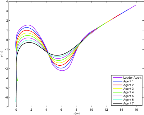
Figure 3: The trajectories on a planar surface of the vehicles composing the platoon.

∎

Remark 2

From the aforementioned proof it can be deduced that the proposed control scheme achieves its goals without resorting to the need of rendering the transformed errors $\varepsilon_{d}\left(\xi_{d}\right)$, $\varepsilon_{\beta}\left(\xi_{\beta}\right)$ arbitrarily small by adopting extreme values of the control gains $K_{d}$, $K_{\beta}$ (see (35) and (37)). The actual performance given in (40) is solely determined by the designer-specified functions $\rho_{d_{i}}\left(t\right),\rho_{\beta_{i}}\left(t\right)$ and parameters $\underline{M}_{d_{i}},\overline{M}_{d_{i}},\underline{M}_{\beta_{i}},\overline{M}_{\beta_{i}}$, that are related to the collision and connectivity constraints. Furthermore, the selection of the control gains $K_{d}$, $K_{\beta}$ is significantly simplified to adopting those values that lead to reasonable control effort. Nonetheless, is should be noted that their selection affects the control input characteristics (i.e., decreasing the gain values leads to increased oscillatory behavior within the prescribed performance envelope described by (5), which is improved when adopting, higher values, enlarging, however, the control effort both in magnitude and rate). Additionally, fine tuning might be needed in real-time scenarios, to retain the required linear and angular velocities within the range that can be implemented by the motors. Similarly, control input constraints impose an upper bound on the required speed of convergence of $\rho_{d_{i}}\left(t\right)$, $\rho_{\beta_{i}}\left(t\right)$ that is affected by the exponentials $e^{-l_{d}t}$, $e^{-l_{\beta}t}$.

IV Simulation Results

To demonstrate the efficiency of the proposed decentralized control protocol, a realistic simulation was carried out in the WEBOTS${}^{\text{TM}}$ platform [31], considering a platoon comprising of a Pioneer3AT/leader and $7$ Pioneer3DX following vehicles. The inter-vehicular distance and the bearing angle are obtained by a camera with range $D=2$m and angle of view $AoV=90^{o}$, that is mounted on each Pioneer3DX vehicle and detects a white spherical marker attached on its predecessor. The leading vehicle performs a smooth maneuver depicted in Fig. 3, along with the trajectories of the following vehicles. The desired distance between successive vehicles is set equally at $d_{i,des}=d=0.75$m,  $i=1,\dots,7$, whereas the collision and connectivity constraints are given by $d_{\mathsf{col}}=0.05d=0.0375$m and $d_{\mathsf{con}}=D=2$m. Regarding the heading error, we select $\beta_{\mathsf{con}}=\frac{AoV}{2}=45^{o}$. In addition, we require steady state error of no more than $0.0625$m and minimum speed of convergence as obtained by the exponential $e^{-0.5t}$ for the distance error. Thus, invoking (7), we select the parameters $\underline{M}_{d_{i}}=0.7125$m$,\overline{M}_{d_{i}}=1.25$m and the functions $\rho_{d_{i}}\left(t\right)=(1-\frac{0.0625}{1.25})e^{-0.5t}+\frac{0.0625}{1.25},$ $i=1,\dots,7$. In the same vein, we require maximum steady state error of $1.15^{o}$ and minimum speed of convergence as obtained by the exponential $e^{-0.5t}$ for the heading error. Therefore, $\underline{M}_{\beta_{i}}=\overline{M}_{\beta_{i}}=\beta_{\mathsf{con}}=45^{o}$ and $\rho_{\beta_{i}}\left(t\right)=(1-\frac{1.15}{45})e^{-0.5t}+\frac{1.15}{45},$ $i=1,\dots,7$. Finally, we chose $K_{d}=\mathrm{diag}[0.005_{,}\dots,0.005]$ and $K_{\beta}=\mathrm{diag}[0.001_{,}\dots,0.001]$ to produce reasonable linear and angular velocities that can be implemented by the motors of the mobile robots.

The simulation results are illustrated in Figs. 4-6. More specifically, the evolution of the distance and heading errors $e_{d_{i}}\left(t\right)$, $e_{\beta_{i}}\left(t\right)$, $i=1,\dots,7$ is depicted in Figs. 4 and 5 respectively, along with the corresponding performance bounds. The inter-vehicular distance along with the collision and connectivity constraints are pictured in Fig. 6. As it was predicted by the theoretical analysis, the decentralized 2-D control problem of vehicular platoons under limited visual feedback is solved with guaranteed transient and steady state response, collision avoidance and connectivity maintenance. Finally, the accompanying video demonstrates the aforementioned simulation study in the WEBOTS${}^{\text{TM}}$ platform.

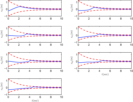
Figure 4: The evolution of the distance errors $e_{d_{i}}(t),i=1,...,7$ (blue lines), along with the imposed performance bounds (red lines).

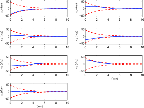
Figure 5: The evolution of the heading errors $e_{\beta_{i}}(t),i=1,...,7$ (blue lines), along with the imposed performance bounds (red lines).

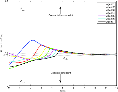
Figure 6: The distance between successive vehicles along with the collision and connectivity constraints.

V Conclusions

We proposed a $2$-D decentralized control protocol for vehicular platoons under the predecessor-following architecture, that establishes arbitrarily fast and maintains with arbitrary accuracy a desired formation without: i) any inter-vehicular collisions and ii) violating the connectivity constraints imposed by the limited field of view of the onboard cameras that are used for visual feedback. Future research efforts will be devoted towards: i) addressing the bidirectional architecture in a similar framework (i.e., prescribed performance as well as collision and connectivity constraints), ii) guaranteeing obstacle avoidance and iii) extending the control protocol to apply for uncertain nonlinear vehicle dynamics. Finally, real-time experiments will be conducted to verify the theoretical findings.

References

- [1] D. Swaroop and J. Hedrick, “String stability of interconnected systems,” Automatic Control, IEEE Transactions on, vol. 41, no. 3, pp. 349–357, Mar 1996.
- [2] T. S. No, K.-T. Chong, and D.-H. Roh, “A lyapunov function approach to longitudinal control of vehicles in a platoon,” Vehicular Technology, IEEE Transactions on, vol. 50, no. 1, pp. 116–124, Jan 2001.
- [3] M. R. Jovanovic and B. Bamieh, “On the ill-posedness of certain vehicular platoon control problems,” IEEE Transactions on Automatic Control, vol. 50, no. 9, pp. 1307–1321, 2005.
- [4] P. Barooah, P. G. Mehta, and J. P. Hespanha, “Mistuning-based control design to improve closed-loop stability margin of vehicular platoons,” IEEE Transactions on Automatic Control, vol. 54, no. 9, pp. 2100–2113, 2009.
- [5] F. Lin, M. Fardad, and M. Jovanovic, “Optimal control of vehicular formations with nearest neighbor interactions,” Automatic Control, IEEE Transactions on, vol. 57, no. 9, pp. 2203–2218, Sept 2012.
- [6] J. Hedrick, M. Tomizuka, and P. Varaiya, “Control issues in automated highway systems,” Control Systems, IEEE, vol. 14, no. 6, pp. 21–32, Dec 1994.
- [7] P. Y. Li, R. Horowitz, L. Alvarez, J. Frankel, and A. M. Robertson, “An automated highway system link layer controller for traffic flow stabilization,” 1997.
- [8] R. Rajamani, H.-S. Tan, B. K. Law, and W.-B. Zhang, “Demonstration of integrated longitudinal and lateral control for the operation of automated vehicles in platoons,” Control Systems Technology, IEEE Transactions on, vol. 8, no. 4, pp. 695–708, Jul 2000.
- [9] H. . Tan, R. Rajesh, and W. . Zhang, “Demonstration of an automated highway platoon system,” in Proceedings of the American Control Conference, vol. 3, 1998, pp. 1823–1827.
- [10] M. Mazo, A. Speranzon, K. Johansson, and X. Hu, “Multi-robot tracking of a moving object using directional sensors,” in Robotics and Automation, 2004. Proceedings. ICRA ’04. 2004 IEEE International Conference on, vol. 2, April 2004, pp. 1103–1108 Vol.2.
- [11] G. Mariottini, G. Pappas, D. Prattichizzo, and K. Daniilidis, “Vision-based localization of leader-follower formations,” in Decision and Control, 2005 and 2005 European Control Conference. CDC-ECC ’05. 44th IEEE Conference on, Dec 2005, pp. 635–640.
- [12] T. Gustavi and X. Hu, “Formation control for mobile robots with limited sensor information,” in Robotics and Automation, 2005. ICRA 2005. Proceedings of the 2005 IEEE International Conference on, April 2005, pp. 1791–1796.
- [13] A. Das, R. Fierro, V. Kumar, J. Ostrowski, J. Spletzer, and C. Taylor, “A vision-based formation control framework,” Robotics and Automation, IEEE Transactions on, vol. 18, no. 5, pp. 813–825, Oct 2002.
- [14] T. Gustavi and X. Hu, “Observer-based leader-following formation control using onboard sensor information,” Robotics, IEEE Transactions on, vol. 24, no. 6, pp. 1457–1462, Dec 2008.
- [15] M. Khatir and E. Davison, “A decentralized lateral-longitudinal controller for a platoon of vehicles operating on a plane,” in American Control Conference, 2006, June 2006, pp. 6 pp.–.
- [16] M. Pham and D. Wang, “A unified nonlinear controller for a platoon of car-like vehicles,” in American Control Conference, 2004. Proceedings of the 2004, vol. 3, June 2004, pp. 2350–2355 vol.3.
- [17] A. Ali, G. Garcia, and P. Martinet, “Minimizing the inter-vehicle distances of the time headway policy for urban platoon control with decoupled longitudinal and lateral control,” in Intelligent Transportation Systems - (ITSC), 2013 16th International IEEE Conference on, Oct 2013, pp. 1805–1810.
- [18] H. Tanner, G. Pappas, and V. Kumar, “Leader-to-formation stability,” Robotics and Automation, IEEE Transactions on, vol. 20, no. 3, pp. 443–455, June 2004.
- [19] J. Lawton, R. Beard, and B. Young, “A decentralized approach to formation maneuvers,” Robotics and Automation, IEEE Transactions on, vol. 19, no. 6, pp. 933–941, Dec 2003.
- [20] D. Maithripala, J. Berg, D. Maithripala, and S. Jayasuriya, “A geometric virtual structure approach to decentralized formation control,” in American Control Conference (ACC), 2014, June 2014, pp. 5736–5741.
- [21] D. Godbole and J. Lygeros, “Longitudinal control of the lead car of a platoon,” Vehicular Technology, IEEE Transactions on, vol. 43, no. 4, pp. 1125–1135, Nov 1994.
- [22] R. Vidal, O. Shakernia, and S. Sastry, “Formation control of nonholonomic mobile robots with omnidirectional visual servoing and motion segmentation,” in Robotics and Automation, 2003. Proceedings. ICRA ’03. IEEE International Conference on, vol. 1, Sept 2003, pp. 584–589 vol.1.
- [23] H. Hao, P. Barooah, and P. G. Mehta, “Distributed control of two dimensional vehicular formations: stability margin improvement by mistuning,” in ASME 2009 Dynamic Systems and Control Conference. American Society of Mechanical Engineers, 2009, pp. 699–706.
- [24] D. Panagou and V. Kumar, “Cooperative visibility maintenance for leader-follower formations in obstacle environments,” Robotics, IEEE Transactions on, vol. 30, no. 4, pp. 831–844, Aug 2014.
- [25] N. Cowan, O. Shakerina, R. Vidal, and S. Sastry, “Vision-based follow-the-leader,” in Intelligent Robots and Systems, 2003. (IROS 2003). Proceedings. 2003 IEEE/RSJ International Conference on, vol. 2, Oct 2003, pp. 1796–1801 vol.2.
- [26] G. Mariottini, F. Morbidi, D. Prattichizzo, G. Pappas, and K. Daniilidis, “Leader-follower formations: Uncalibrated vision-based localization and control,” in Robotics and Automation, 2007 IEEE International Conference on, April 2007, pp. 2403–2408.
- [27] G. Mariottini, F. Morbidi, D. Prattichizzo, N. Vander Valk, N. Michael, G. Pappas, and K. Daniilidis, “Vision-based localization for leader-follower formation control,” Robotics, IEEE Transactions on, vol. 25, no. 6, pp. 1431–1438, Dec 2009.
- [28] C. P. Bechlioulis, D. V. Dimarogonas, and K. J. Kyriakopoulos, “Robust control of large vehicular platoons with prescribed transient and steady state performance,” in Proceedings of the IEEE Conference on Decision and Control, 2014, Accepted.
- [29] C. P. Bechlioulis and G. A. Rovithakis, “A low-complexity global approximation-free control scheme with prescribed performance for unknown pure feedback systems,” Automatica, vol. 50, no. 4, pp. 1217–1226, 2014.
- [30] E. D. Sontag, Mathematical Control Theory. London, U.K.: Springer, 1998.
- [31] Cyberbotics, “Webots: A commercial Mobile Robot Simulation Software,” http://www.cyberbotics.com, Online.