Random Switching between Vector Fields Having a Common Zero
Abstract
Let be a finite set, a family of vector fields on leaving positively invariant a compact set and having a common zero We consider a piecewise deterministic Markov process on defined by where is a jump process controlled by for on
We show that the behavior of is mainly determined by the behavior of the linearized process where is the Jacobian matrix of at and is the jump process with rates We introduce two quantities and respectively defined as the minimal (respectively maximal) growth rate of where the minimum (respectively maximum) is taken over all the ergodic measures of the angular process with It is shown that coincides with the top Lyapunov exponent (in the sense of ergodic theory) of and that under general assumptions We then prove that, under certain irreducibility conditions, exponentially fast when and converges in distribution at an exponential rate toward a (unique) invariant measure supported by when Some applications to certain epidemic models in a fluctuating environment are discussed and illustrate our results.
Keywords:
Piecewise deterministic Markov processes; Random Switching; Lyapunov Exponents; Stochastic Persistence; Hypoellipticity, H rmander-Bracket conditions; Epidemic models; SIS
AMS subject classifications
60J25, 34A37, 37H15, 37A50, 92D30
1 Introduction
Let be a finite set and a family of globally integrable vector fields on For each we let denote the flow induced by We assume throughout that there exists a closed set which is positively invariant under each That is
for all
Consider a Markov process living on whose infinitesimal generator acts on functions smooth in the first variable, according to the formula
| (1) |
where stands for and is an irreducible rate matrix continuous in Here, by a rate matrix, we mean a matrix having nonnegative off diagonal entries and zero diagonal entries.
In other words, the dynamics of is given by an ordinary differential equation
| (2) |
while is a continuous time jump process taking values in controlled by
where
This class of processes belongs to the wider class of Piecewise Deterministic Markov Processes (PDMPs), a term coined by Davis [24], and has recently been the focus of much attention. Criteria, based on irreducibility and Hörmander type conditions, ensuring uniqueness and absolute continuity of an invariant probability measure have been obtained by Bakhtin and Hurth [5] for constant jump rates ( and by Benaïm, Le Borgne, Malrieu and Zitt [16] for more general rates. Exponential convergence (in total variation) toward this measure and a support theorem, describing the support of the law of are also proved in [16] when is compact (see also [13]). In the one dimensional case (i.e ) smoothness properties of the invariant measure are thoroughly investigated by Bakhtin, Hurth and Mattingly [6]. When irreducibility fails to hold, the support of invariant probabilities can be determined in terms of invariant control sets of an associated deterministic control system (see Benaïm, Colonius and Lettau [10]). When the vector fields are exponentially asymptotically stable in "average", exponential convergence toward an invariant measure are obtained for Wassertein distances by Benaïm, Le Borgne, Malrieu and Zitt [14], Cloez and Hairer [21]. Several examples, either linear (Benaïm, Le Borgne, Malrieu and Zitt [15], Lawley, Mattingly and Reed [36], Lagasquie [34]), or nonlinear (Benaïm and Lobry [17], Malrieu and Hoa Phu [38]) show that the behavior of the process is not solely determined by the dynamics of the but can be highly sensitive to the switching rates. We refer the reader to the recent overview by Malrieu [37], describing these results among others.
In the present paper we will investigate the behavior of the process under the following two conditions:
- C1
-
The origin lies in and is a common equilibrium:
- C2
-
The set is compact and locally star shaped at the origin, meaning that there exists such that
where .
Compactness of is assumed here for simplicity, but some of the (local) results generalise to noncompact sets. The global results can be extended provided we can control the behaviour of the process near infinity, for instance with a suitable Lyapunov function (see Section 3.3).
Briefly put, our main result is that the long term behavior of the process is determined by the behavior of the process obtained by linearization at the origin and, under suitable irreducibility and hypoellipticity conditions, by the top Lyapunov exponent of the linearized system. If negative, then converges almost surely and exponentially fast to zero. If positive, and the empirical occupation measure (respectively the law) of converge almost surely (respectively in total variation at an exponential rate) toward a unique probability measure putting zero mass on Such a correspondence between the sign of the top Lyapunov exponent and the behavior of nonlinear system is reminiscent of the results obtained by Baxendale [7] and others for Stratonovich stochastic differential equations (see [7] and the references therein, and Hening, Nguyen and Yin [31] for similar recent results in the context of population dynamics).
Our proofs rely, on one hand, on the qualitative theory of PDMPs (as developed in [5] and [16]) and, on the other hand, on some recent results on stochastic persistence (Benaïm [9]) strongly inspired by the seminal works of Schreiber, Hofbauer and their co-authors on persistence, first developed for purely deterministic systems (Schreiber [42], Garay and Hofbauer [27], Hofbauer and Schreiber [33]) and later for certain stochastic systems (Benaïm, Hofbauer and Sandholm [12], Benaïm and Schreiber [18], Schreiber, Benaïm and Atchade [44], Schreiber [43], Roth and Schreiber [41]).
Our original motivation was to analyze the behavior of certain epidemic models evolving in a fluctuating environment. A famous, and now classical, deterministic model of infection is given by the Lajmanovich and Yorke differential equation ([35]). This equation leaves positively invariant the unit cube of and models the evolution of the infection level between groups. Depending on the parameters of the model (the environment), either the disease dies out (i.e all the trajectories converge to the origin) or stabilizes (i.e all non zero trajectories converge toward a unique positive equilibrium). Deterministic switching between several environment have been recently considered by Ait Rami, Bokharaie, Mason and Wirth [1]. The results here allow to describe the behavior of the process when switching between environment evolves randomly. In particular we can produce paradoxical examples for which, although each deterministic dynamics leads to the extinction (respectively persistence) of the disease, the random switching process leads to persistence (respectively extinction) of the disease.
1.1 Outline of contents
Section 2 considers the linearized system where (the Jacobian of at ) and is the jump process with rate matrix We introduce two quantities and respectively defined as the minimal (respectively maximal) growth rate of where the minimum (respectively maximum) is taken over all the ergodic measures of the angular Markov process with It is shown (Proposition 2.5) that coincides with the top Lyapunov exponent (in the sense of ergodic theory) of and some conditions are given ensuring that first for arbitrary s (Proposition 2.11) and then for Metzler matrices (Proposition 2.13).
The main results of the paper are stated in Section 3.
-
•
If exponentially fast, locally (i.e for small enough), with positive probability. If furthermore is accessible, convergence is global and almost sure (Theorem 3.1).
-
•
If and , the process is persistent in the sense that weak limit points of its empirical occupation measure are almost surely invariant probabilities over (Theorem 3.2). If in addition the s satisfy a certain Hörmander-type bracket condition at some accessible point, then there is a unique invariant probability on toward which the empirical occupation measure converges almost surely (Theorem 3.3). Under a strengthening of the bracket condition, the distribution of the process converges also exponentially fast in total variation (Theorem 3.4).
Section 4 discusses some applications of our results to certain epidemic models in a fluctuating environment. The focus is on the situation where the s are given by Lajmanovich and Yorke type vector fields [35] (or more generally sub homogeneous cooperative systems in the sense of Hirsch [32]). Several examples are analyzed and a theorem proving exponential convergence of the distribution (for a certain Wasserstein distance) in absence of the bracket condition is stated (Theorem 4.12).
1.2 Notation
The following notation will be used throughout: denotes the Euclidean inner product in the associated norm, the closed ball centered at with radius and the unit sphere.
Notation for Markov processes
For any polish space such as equipped with its Borel sigma-field, we let denote the set of (Borel) probabilities over We shall consider below certain Markov processes (like ) taking values in with cad-lag (right continuous, left limit) paths. Given such a process and we let denote the law of on the Skorokhod space when has law As usual, stands for for all The Markov semi-group induced by denoted acts on bounded measurable functions according to the formula
By duality it acts on by
where here and throughout stands for Probability is said invariant for provided for all It is called ergodic if, in addition of being invariant, the only bounded measurable functions for which are -almost surely constant.
We let denote the (possibly empty) set of invariant probabilities of and the subset of ergodic probabilities. Recall that can also be defined as the set of extremal points of
A key property, that will be used later without further notice, is that whenever (respectively ), is invariant (respectively ergodic), in the sense of ergodic theory, for the shift on where
We refer the reader to Meyn and Tweedie ([39], chapter 17) for a proof and more details.
Accessibility
Let be a family of bounded vector fields on indexed by For instance We let denote the compact convex set valued mapping defined by
Given a closed set and we say that is -accessible from if for every neighborhood of and every there exists a (absolutely continuous) function solution to the differential inclusion
such that for some . An equivalent formulation (see e.g Theorem 2.2 in [10]) is that is reachable from by the control system
where the control with the canonical basis of Note that this notion is what is called -approachability in [5].
2 The Linearized system
Let, for denote the Jacobian matrix of at the origin. We let denote the cone defined as
where is like in condition Here, stands for the closure of .
Remark 2.1
One can check that the definition of does not depend on the choice of , provided satisfies condition .
Lemma 2.2
For all
Proof We set and first prove that The lemma will be then induced by continuity of . Let For small enough, by definition of and continuity of at
Hence and letting this shows that
QED
Define the linearized system of at the origin as the "linear" PDMP living on whose generator is given by
where
A trajectory with initial condition is then obtained as a solution to
| (3) |
where is a continuous time Markov process on with jump rates based at
By irreducibility of has a unique invariant probability characterized by
Whenever the polar decomposition
is well defined and (3) can be rewritten as
| (4) |
where for all is the vector field on defined by
| (5) |
Remark 2.3
For stochastic differential equations, the idea of introducing, this polar decomposition goes back to Hasminskii [30] and has proved to be a fundamental tool for analyzing linear stochastic differential equations (see e.g [7]), linear random dynamical systems (see e.g chapter 6 of Arnold [2]) and more recently certain linear PDMPs in [15], [36] or [34].
With obvious notation, the processes
and
are two PDMPs respectively living on and
By compactness of and Feller continuity of (see [16], Proposition 2.1), is a nonempty compact (for the topology of weak* convergence) subset of
2.1 Average growth rates
Define, for each the -average growth rate as
| (6) |
where is the measure on defined by
Note that when is ergodic, by equation (4) and Birkhoff ergodic theorem
almost surely.
Define similarly the extremal average growth rates as the numbers
| (7) |
The following rough estimate is a direct consequence of (6). Recall that is the invariant probability of
Lemma 2.4
where (respectively ) denotes the smallest (respectively largest) eigenvalue.
The signs of and will play a crucial role for determining the asymptotic behavior of the non linear process But before stating our main results, it is interesting to compare them with the usual Lyapunov exponents given by the multiplicative ergodic theorem.
2.2 Relation with Lyapunov exponents
Set and for and let
denote the solution to the linear differential equation
with initial condition
Then, is a linear random dynamical system over the ergodic dynamical system for which the assumptions of the multiplicative ergodic theorem are easily seen to be satisfied (see e.g [2], Theorem 3.4.1 or Colonius and Mazanti [22]). Thus, according to this theorem, there exist numbers
called the Lyapunov exponents of , a Borel set with and for each distinct vector spaces
(measurable in ) such that
| (8) |
for all .
Proposition 2.5
For all
If furthermore has non empty interior, then
Remark 2.6
The second part of the proposition has already been proven by Crauel [23, Theorem 2.1 and Corollary 2.2] in a more general setting. We adapt the arguments of his proof for our specific case.
Proof Let Then, almost surely
The first equality follows from (3), (4) and the definition of The second follows from Birkhoff ergodic theorem. Therefore, there exists a Borel set such that for all
| (9) |
and where is the law of under
Let be the set given by the multiplicative ergodic theorem and Then Hence and for all the left hand side of equality (9) equals for some
It remains to show that . For every in the set given by the multiplicative ergodic theorem, and for all , define
where
By (8), we have for all . Let denote the normalised Lebesgue measure on . Because is at most an hyperplane and has non empty interior, we get that for all . In particular,
| (10) |
Moreover, because , dominated convergence and (10) imply that
| (11) |
Now for all , define the probability on
| (12) |
By compactness of , is tight, and by Feller property of , every weak limit points of belongs to . Let be such a limit point, and such that . Setting , one has . Now (9), (11) and Fubini Theorem imply that , which concludes the proof.
QED
In the multiplicative ergodic theorem, each Lyapunov exponent comes with an integer called its multiplicity and such that (see Chapter 3 of [2] for more details). A consequence of Proposition 2.5 is the following inequality which provides, in some cases, a simple way to prove that , which is often a sufficient condition to ensure positive recurrence of on (see Propostions 2.11 and 2.13 and Theorems 3.2 and 3.3).
Corollary 2.7
Proof By Jacobi’s formula
By Birkhoff ergodic Theorem, the right hand side of this equality converges, almost surely, as toward and a by product of the multiplicative ergodic theorem (see e.g [2], Chapter 3, Corollary 3.3.4) is that the left-hand side converges almost surely,
as toward
QED
Remark 2.8
Remark 2.9
Note that in general
Here is a simple example based on [15]. Assume and (so that the matrices here are ). Let be real matrices having eigenvalues with negative real parts and such that for some the eigenvalues of have opposite signs. It is not hard to construct such a matrix (see e.g [15], Example 1.3). Suppose and with so that Then, by Corollary 2.7, the Lyapunov exponents, (counted with their multiplicity) satisfy
while, it follows from Theorem 1.6 of [15], that for sufficiently large. Hence (for large )
2.3 Uniqueness of average growth rate
In this section we discuss general conditions ensuring that
A sufficient condition is given by unique ergodicity of meaning that has cardinal one. However, whenever is symmetric (i.e ), for each there is another (possibly equal) invariant measure given as the image measure of by the map Indeed, it is easy to see that
for all This follows from the equivariance property
satisfied by the (see equation 5). Clearly Thus, when is symmetric, a (weaker than unique ergodicity) sufficient condition is that the quotient space obtained by identification of with has cardinal one.
Example 2.10 (One dimensional systems)
Suppose and Thus and where and Hence where .
The two following results complement the previous discussion with practical conditions.
Set where is the Lie bracket operation. Following [16], we say that the weak bracket condition holds at provided the vector space spanned by the vectors has full rank (i.e ).
Proposition 2.11
Assume there exists such that
- (i)
-
The weak bracket condition holds at
- (ii)
-
Either is -accessible from or, is symmetric and is -accessible from
Then in the first case, and in the second, has cardinal one. In particular
Proof Existence of an invariant probability follows from compactness and Feller continuity. By Theorem 1 in [5] or Theorem 4.4 in [16] Condition and accessibility of imply that such a measure is unique (and absolutely continuous with respect to ). In case is symmetric and accessible, let be the projective space obtained by identifying each point with the antipodal point and the quotient map. The PDMP induces a PDMP on for which is accessible and at which the weak bracket condition holds. The preceding results applies again.
QED
Example 2.12 (Two dimensional systems)
Suppose and that one of the two following conditions is verified :
- (a)
-
At least one matrix, say , has no real eigenvalues; or
- (b)
-
at least two matrices, say have no (nonzero) common eigenvector.
Then the assumptions, hence the conclusions, of Proposition 2.11 hold.
Indeed, under condition , the flow induced by is periodic on so that every point satisfies the assumptions of Proposition 2.11. Under condition , let be the eigenvalues of and corresponding eigenvectors. If is an attractor for the flow induced by whose basin is Since is accessible and since assumption of Proposition 2.11 is satisfied at point If every trajectory of the flow induced by converges either to or and the preceding reasoning still applies.
The next proposition will be useful in Section 4 for analyzing random switching between cooperative vector fields and certain epidemiological models. In case the matrices are irreducible, this proposition follows from the Random Perron-Frobenius theorem as proved by Arnold, Demetrius and Gundlach in [3]. However, to handle the weaker assumption the proof needs to be adapted, but relies on the same ideas. Details are given in Section 7. Recall (see remark 2.8) that a Metzler matrix is a matrix with nonnegative off-diagonal entries. We say that such a matrix is irreducible if adding a sufficiently large multiple of the identity, the obtained matrix is a non-negative irreducible matrix in the usual sense.
Proposition 2.13
Assume that
- (i)
-
- (ii)
-
For each is Metzler,
- (iii)
-
There exists (i.e ) such that
is irreducible.
Then has cardinal one. In particular
2.4 Average growth rate under frequent switching
The definition of average growth rates (see equations (6) and (7)) involve the invariant measures of whose explicit computation may prove highly difficult if not impossible. However, when switchings occur frequently, such measures can, by a standard averaging procedure, be estimated by the invariant measures of the mean vector field; i.e the vector field obtained by averaging.
More precisely, we have the following Lemma :
Lemma 2.14
Assume the switching rates are constant and depend on a small parameter where is an irreducible matrix with invariant probability . Denote by the associated PDMP given by (4), and for any , let be an element of Then, every limit point of in the limit is of the form , where is an invariant probability measure of the flow induced by .
The proof of this lemma follows from standard averaging results. Details are given in Section 7. An immediate corollary is :
Corollary 2.15
With the hypotheses of Lemma 2.14, assume that the flow induced by admits a unique invariant measure on . Denote by and the extremal growth rates of . Then
In particular, if is Metzler and irreducible, then it admits a unique eigenvector on and
3 The non linear system : Main results
3.1 Extinction
The first result is an extinction result.
Theorem 3.1
Assume Let Then there exists a neighborhood of and such that for all and
If furthermore is -accessible from then for all and
3.2 Persistence
The next results are persistence results obtained under the assumption that
We let
denote the empirical occupation measure of the process For every Borel set
is then the proportion of the time spent by in up to time
We let
Theorem 3.2
Assume Then the following assertions hold:
- (i)
-
For all there exists such that for all , , almost surely,
In particular, for all almost surely, every limit point (for the weak* topology) of belongs to
- (ii)
-
There exist positive constants such that for all
- (iii)
-
Let and be the stopping time defined by
There exist , and such that for all and ,
Set and where is the Lie bracket operation. We say (compare to Section 2.3) that the weak bracket condition holds at provided the vector space spanned by the vectors has full rank. We let denote the Lebesgue measure on
Theorem 3.3
In addition to the assumption assume that there exists a point -accessible from at which the weak bracket condition holds. Then
- (i)
-
The set reduces to a single element, denoted ;
- (ii)
-
is absolutely continuous with respect to ;
- (iii)
-
For all and ,
almost surely.
In order to get a convergence in distribution of the process , the weak bracket condition needs to be strengthened. Set and We say that the strong bracket condition holds at provided the vector space spanned by the vectors has full rank.
Given the total variation distance between and is defined as
where the supremum is taken over all Borel sets
Theorem 3.4
Under the conditions of the preceding theorem, assume furthermore that one the two following holds :
- (i)
-
The weak bracket condition is strengthened to the strong bracket condition; or
- (ii)
-
There exist with and a point -accessible from such that .
Then there exist such that for all and ,
3.3 The noncompact case
We briefly discus here the situation where is not compact. First, note that all the results given in section 2 still hold, because they only deal with the linearised system. Next, local statements remain true without additional assumption by a localisation argument. Namely :
Theorem 3.5
-
1.
Assume Let Then there exists a neighborhood of and such that for all and
-
2.
Assume Then there exist , and such that for all and ,
To extend the global results stated above , we make the additional assumption that the jumps rates are bounded and that there exists a Lyapunov function, controlling the behaviour of the process at infinity.
Hypothesis 3.6
The jumps rate are bounded :
For a function , we denote by the function defined by :
We also let denote the space of functions that are constant outside a compact set and in the first variable.
Hypothesis 3.7
There exists a continuous function with , a continuous function , and such that
-
(i)
For every compact set , there exists such that
-
(a)
and ,
-
(b)
For all ,
-
(a)
-
(ii)
Theorem 3.8
Example 3.9
We consider a random switching between two linear systems given by Metzler matrices and , with transition rate . We assume that has two distinct positive eigenvalues and is irreducible, whereas is of the form
with . Since the eigenvalues of are positive, there is no invariant compact set for , nor for the PDMP. Moreover, and being Metzler, is positively invariant for . If the jump rates were constant in , the process would either converge to or to infinity. To ensure positive recurrence on , we assume that the transition rates are such that, near the origin, spends more time in state :
| (13) |
While near infinity, it spends more time in state :
| (14) |
More precisely, we have the following :
Proposition 3.10
Proof By Theorem 2.13, , and by Corollary 2.7,
Moreover, it is easy to check that and . Hence, if , then . Now we show that we can construct a Lyapunov function at infinity. Let and and define, for all , . Formally, we have
By assumption on and , and . Hence,
where and . First we prove that we can choose and such that satisfies point (ii) of Hypothesis 3.7 for all small enough. Then we prove that we can choose such that point (i-b) holds. By assumption (14), there exists and such that, for all with , . This implies that, for small enough, there exists such that , which yields
Now we choose and such that
Thus, for , . In particular, for all for , . Since is bounded for , then for some constant (depending on ). This has the consequence (see [9, Theorem 2.1]) that for all ,
| (15) |
The computation of gives
hence
for some constant . Hence, choosing small enough so that (15) holds for , one has
which proves (i-b). It remains to show that there exist accessible points at which the strong bracket condition holds. Set and the vector fields associated to and . There exist , with such that . Straightforward computations show that
Since , this polynomial is non identically null. To conclude, we prove that there exists an open set of accessible points. Let be the Perron eigenvector associated with . We claim that and therefore are accessible. One can check that for all and all , there exists such that for all with , there exists such that . Since is accessible following , this makes accessible. Hence, is accessible and Theorem 3.8 applies. QED
4 Epidemic Models in Fluctuating Environment
We discuss here some implications of our results to certain epidemics models evolving in a randomly fluctuating environment.
Forty years ago, Lajmanovich and Yorke in a influential paper [35], proposed and analyzed a deterministic SIS (susceptible-infectious-susceptible) model of infection, describing the evolution of a disease that does not confer immunity, in a population structured in groups. The model is given by a differential equation on (the unit cube of ) having the form
| (16) |
where is an irreducible matrix with nonnegative entries and Here represents the proportion of infected individuals in group is the intrinsic cure rate in group and is the rate at which group transmits the infection to group Irreducibility of implies that each group indirectly affects the other groups. By a classical mean field approximation procedure, (16) can be derived from a finite population model, in the limit of an infinite population (see Benaïm and Hirsch [11]).
Here and throughout, for any matrix we let denote the largest real part of the eigenvalues of A matrix is called Hurwitz provided . Lajmanovich and Yorke [35] prove the following result:
Theorem 4.1 (Lajmanovich and Yorke, [35])
Let
If is globally asymptotically stable for the semiflow induced by (16) on
If there exists another equilibrium whose basin of attraction is
In this epidemiological framework, is called the disease free equilibrium, and the point , when it exists, the endemic equilibrium. It turns out that such a dichotomic behavior is very robust to the perturbations of the model and can be obtained under a very general set of assumptions, using Hirsch’s theory of cooperative differential equations.
We let denote the interior of the non negative orthant For we write (or ) if if and and if
Following [11] (especially Section 3), we call a map an epidemic vector field if it is continuously differentiable111by this we mean that can be extended to a vector field on and satisfies the following set of conditions:
- E1
-
- E2
-
- E3
-
is cooperative i.e the Jacobian matrix is Metzler for all
- E4
-
is irreducible on i.e is irreducible for all
- E5
-
is strongly sub-homogeneous on i.e for all and
It is easy to verify that the Lajmanovich and Yorke vector field (given by the right hand side of (16)) satisfies these conditions.
Let denote the local flow induced by Condition has the important consequence that for all is monotone for the partial ordering That is if In particular, by for all Combined with this shows that is positively invariant under
The following result shows that trajectories of behave exactly like the trajectories of the Lajmanovich and Yorke system. The first assertion was stated in ([11], Theorem 3.2) but its proof is a consequence of more general results due to Hirsch (in particular Theorems 3.1 and 5.5 in [32]).
Theorem 4.2
Let be an epidemic vector field and the induced semiflow on Then
- (i)
-
(Hirsch, [32]) Either is globally asymptotically stable for ; or there exists another equilibrium whose basin of attraction is
- (ii)
-
Let Then is globally asymptotically stable if and only if
Proof As already mentioned, follows from [32], Theorems 3.1 and 5.5. We detail the proof of . If then is linearly stable hence globally stable by If there exists, by irreducibility and Perron Frobenius theorem, such that Hence for small enough, because as Consequently is positively invariant and cannot be asymptotically stable.
It remains to show that is asymptotically stable when Suppose the contrary. By there exists another equilibrium Set By strong subhomogeneity, Let For all is an epidemic vector field and is linearly stable for (because ). On the other hand, for small enough, so that the set is positively invariant by A contradiction.
QED
4.1 Fluctuating environment
We consider a PDMP as defined in Section 1, under the assumptions that:
- E’1
-
- E’2
-
For all is Metzler;
- E’3
-
There exists such that the convex combination is irreducible.
Observe that these conditions are automatically satisfied if consists of epidemic vector fields but are clearly much weaker.
Relying on Proposition 2.13, we let denote the top Lyapunov exponent of the linearized system.
Theorem 4.3
Assume and that one of the following two conditions holds:
- (a)
-
The jump rates are constant (i.e and the are epidemic; or
- (b)
-
There exists such that is epidemic and
Then for all and ,
Proof We first prove the result under condition Recall (see Section 2.2) that stands for For each and let
be the solution to the non autonomous differential equation
with initial condition By conditions and each flow is monotone and subhomogenous (see e.g [32], Theorem 3.1). The composition of monotone subhomogeneous mappings being monotone and subhomogeneous, is monotone and subhomogeneous for all and Thus, for all and
| (17) |
Under the assumption that the jump rates are constant, is the image measure of by the map
Therefore, by Theorem 3.1, there exists such that for all
| (18) |
Combined with (17), this proves that (18) holds true not only for but for all A standard application of the Markov property then implies the result.
Under condition , it follows from Theorem 4.2, that is -accessible from , and the result follows from Theorem 3.1.
QED
Remark 4.4
The assumption made in case that the are epidemic can be weakened. The proof shows that irreducibility of is unnecessary and that strong subhomogeneity can be weakened to subhomogeneity.
Remark 4.5
Case (and its proof) can be related with the results obtained by Chueshov in [20], for SIS models with random coefficients (see [20, Section 5.7.2]) and, more generally, for monotone subhomogeneous random dynamical systems. Note, however, that in comparison with Chueshov’s approach, in case there is no assumption that the s are monotone nor subhomogeneous.
Example 4.6 (Fluctuations may promote cure)
We give here a simple example consisting of two Lajmanovich-Yorke vector fields modeling the evolution of an endemic disease (each vector field possesses an endemic equilibrium) but such that a random switching between the dynamics leads to the extinction of the disease.
Suppose Let be the Lajmanovich-Yorke vector fields respectively given by
and
One can easily check that
so that for each there is an endemic equilibrium and the disease free equilibrium is a repellor. On the other hand,
so that the disease free equilibrium is a global attractor of the average vector field Consider now the PDMP given by constant switching rates
By Corollary 2.15, this implies that provided is sufficiently large. Thus the conclusion of Theorem 4.3 holds.
Example 4.7 (Fluctuations may promote infection)
We give here another simple example consisting of two Lajmanovich-Yorke vector fields for which the disease dies out, but such that a random switching between the dynamics leads to the persistence of the disease.
With the notation of Example 2, assume now that
and
Straightforward computation shows that
and that the endemic equilibrium of is the point Then is - accessible and one can easily check that the strong bracket condition holds at . Thus, for sufficiently large, this implies by Corollary 2.15 and Theorem 3.4 the exponential convergence in total variation of the distribution of (whenever ) towards a unique distribution absolutely continuous with respect to and satisfying the tail condition given by Theorem 3.2 (ii). Furthermore, it follows from ([16], Proposition 3.1) that the topological support of writes where is a compact connected set containing both and , and whose interior is dense in .
Remark 4.8
In [13], we show that the previous example can be generalised in the following way. Assume that and are two epidemic vector fields in dimension such that
-
1.
and ,
-
2.
There exists such that , where .
Then, [13, Lemma 3.7] show that there exists an accessible point at which the weak bracket condition holds. Moreover, since , Theorem 4.2 implies that condition (ii) of Theorem 3.4 is satisfied. Thus, by this theorem, we can conclude that there is convergence in total variation to a unique invariant probability measure provided . This happens for example with switching rates of the form
for large enough (by Corollary 2.15.)
Remark 4.9
In the preceding example, the matrices are Metzler and Hurwitz but because the convex hull of the contains a non Hurwitz matrix. This leads to the natural question of finding examples for which:
and every matrix in the convex hull of the is Hurwitz.
For arbitrary (i.e non Metzler) matrices, such and example has been given in dimension 2 in [36] and more recently in [34].
Now, if we restrain ourselves to Metzler matrices, a result from Gurvits, Shorten and Mason ([28, Theorem 3.2]) proves that, in dimension 2, when every matrix in the convex hull is Hurwitz, then is globally asymptotically stable for any deterministic switching between the linear systems. In particular, this implies that cannot be positive.
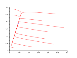
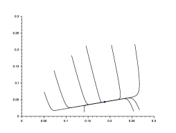
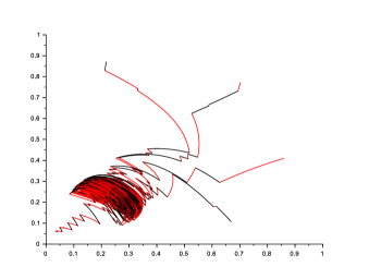
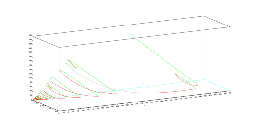
However, they show that it is possible in some higher dimension to construct an example where all the matrices in the convex hull are Hurwitz, and for which there exists a periodic switching such that the linear system explodes. Later, an explicit example in dimension 3 was given by Fainshil, Margaliot and Chiganski [25]. Precisely, consider the matrices
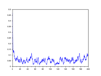
It is shown in [25] that every convex combination of and is Hurwitz, and yet a switch of period 1 between and yields an explosion. Some simulations made on Scilab (see Figure 5) let us think that this result is still true for a random switching, with rates
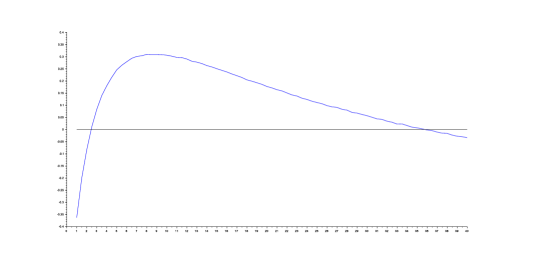
Here has to be chosen neither too small nor too big. Using the formula
and Monte-Carlo simulations we can estimate numerically The results are plotted in Figure 6 and show (although we didn’t prove it) that for providing a positive answer to the question raised at the beginning of the remark.
Example 4.10 (Fluctuations may promote infection, continued)
Remark 4.9 can be used to produce two Lajmanovich-Yorke vector fields on such that
- (i)
-
For all the disease free equilibrium is a global attractor of the vector field
- (ii)
-
A random switching between the dynamics leads to the persistence of the disease.
Observe that is the Lajmanovich-Yorke vector field with infection matrix and cure rate vector
To do so, one just has to choose in such way that . For the simulation given here, we have chosen
and
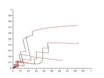
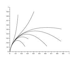
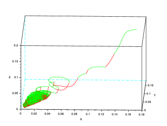
When (see Figure 6) is such that , then by Theorem 4.12 below, admits a unique invariant measure on . Moreover by Theorem 3.2, there exists such that
Figure 7 and 8 illustrate this persistence of the infection. In figure 8 , we have plotted .
4.2 Exponential convergence without bracket condition
Throughout this section, we assume that the vector fields are epidemic and that the jump rates are constant. Recall (see proof of Theorem 4.3) that this implies that for all and , is monotone and strongly subhomegeneous. A very useful consequence of this fact is the strict nonexpansivity of on with respect to the Birkhoff part metric , the definition of which is recalled below. Now if we assume that , we have a Lyapunov function and nonexpansivity, so we might expect uniqueness of the invariant measure on and convergence in law of towards it. Here we prove that this is indeed the case, and even that we have an exponential rate of convergence towards this invariant measure for a certain Wasserstein distance, thanks to a weak form of Harris’ theorem given by Hairer, Mattingly and Scheutzow [29]. But before to do so, we explain briefly why we cannot expect to have convergence in total variation without additional assumptions with the following simple example :
Example 4.11
Suppose Let be the Lajmanovich-Yorke vector fields respectively given by
and
One can easily check that the point is a common equilibrium of and . In particular, is an invariant probability of Moreover, for all , and , one has so for all . Now let us quickly show that converges almost surely exponentially fast to , for all switching rates. Let (respectively ) denote the top Lyapunov exponent of the linearized system at the origin (respectively at ). By Proposition 2.13 this exponent coincides with the unique average growth rate of the corresponding linearized system. We claim that and The first inequality follows from the Kolotilina-type lower estimate for the top Lyapunov exponent mentioned in Remark 2.8 due to Mierczyński ([40, Theorem 1.3]). In our setting, this estimate ensures that
which is positive because and the other terms are positive. Let Then the second estimate follows from Lemma 2.4 because one can easily check that . So applying Theorem 3.1, we have a neighborhood of and such that for all and
| (19) |
On the other hand, because , there exists by Theorem 3.2 such that for all ,
| (20) |
where . Finally, because is a linear stable equilibrium for with basin of attraction contains , one can show that there exists a constant such that for all with ,
| (21) |
Combining (19), (20), (21) and the Markov property implies that
for all (see [17, Theorem 3.1] for details on a very similar proof).
Before stating our theorem, recall the definition of the Wasserstein distance. Let be a Polish space, and be a distance-like function on . That is satisfies the axioms of a distance, except for the triangle inequality. Then the Wasserstein distance associated to is defined for every by
where is the set of all the coupling of and . When is a distance, so is , and in every case, if and only if .
Set .
Theorem 4.12
Assume the are epidemic vector fields, are constant and . Then there exists a distance-like function , and , such that,
- (i)
-
for all , for all ,
- (ii)
-
has a unique invariant measure on , and for all ,
5 Proofs of Theorems 3.1–3.4 : A stochastic persistence approach
As indicated in the introduction, the proofs will be deduced from the qualitative properties of PDMPs combined with general results on stochastic persistence proved in [9] along the lines of the seminal results obtained by Schreiber, Hofbauer and their co-authors for deterministic systems.
5.1 An abstract stochastic persistence result
The results in [9] concern certain Markov processes on a (possibly) non compact metric space satisfying a weak version of the Feller property. Here for simplicity we shall state a simpler version of these results tailored for Feller processes on a compact space.
Let be a compact metric space and a cad-lag Markov process on To shorten notation we write in place of . We let
denote the empirical occupation measure of We let denotes the space of real valued continuous functions on equipped with the uniform norm
We assume that is Feller. That is
- (a)
-
For all maps into itself,
- (b)
-
For all
We let denote the infinitesimal generator of and its domain. Recall that is defined as the set of such that converges in and, for such an denotes the limit. We let denote the set of such that For the Carré du champ of is defined as
| (22) |
We assume that
Hypothesis 5.1
there exists a non empty compact set called the extinction set which is invariant under That is
where stands for the indicator function of
We set
etc.
Extinction of amounts to say that trajectories of converge almost surely to Let be the -neighborhood of Using a terminology borrowed to Schreiber [43] and Chesson [19], we say that is stochastically persistent (or almost surely persistent), respectively persistent in probability, provided
almost surely for all Respectively
for all
General criteria ensuring extinction or persistence are given by the existence of a suitable average Lyapounov function as defined now.
In addition to hypothesis 5.1 we assume that
Hypothesis 5.2
There exist continuous maps and enjoying the following properties :
- (a)
-
For all compact there exists with and
- (b)
-
- (c)
-
- (d)
-
Jumps of are bounded : such that
Let Define the -exponents of the processes as
We call the process -persistent if and -nonpersistent if
By the Ergodic decomposition theorem, note that (respectively ) if and only if (respectively ) for all
We say that is accessible from if for every neighborhood of and there exists such that
We call a point a Doeblin point provided there exists a neighborhood of , a bounded (positive) measure on and some number such that
for all The following theorem is a consequence of Theorems 4.4 and 4.10 and Proposition 8.2 in [9].
Theorem 5.3
Suppose that the process is -persistent. Then
- (i)
-
The process is stochastically persistent. In particular, for all almost surely, every limit point of lies in
- (ii)
-
There exist and positive constants such that
- (iii)
-
Let and be the stopping time defined by
Then there exists such that for all , there exists such that for all
- (iv)
-
If, furthermore, there exists a Doeblin point accessible from then reduces to a single measure and for all
for some
The next result is a general extinction result.
Theorem 5.4
Suppose that the process is -nonpersistent. Then
- (i)
-
For all , there exists a neighborhood of and such that
for all
- (ii)
-
If furthermore is accessible from
for all
Proof Since the proof is very similar to the one given in [17, Theorem 3.1], we only give a sketch of it. Let . The proofs of Propositions 8.2 and 8.3 in [9] (see also [17, Lemma 3.5]) adapt verbatim in the nonpersistent case to prove that there exist , , and such that, for all ,
-
(i)
,
-
(ii)
.
Here and throughout this proof, . We set . We claim that
-
1.
There exists such that for all , ;
-
2.
On the event , and for all , .
In particular, this implies point (i) of the Theorem with Point (ii) easily follows by Markov property. We prove the first claim. We set for , . Due to point (ii) above, is a supermartingale. In particular, for all ,
By dominated convergence, this gives
which proves the first point with . We now prove the second claim. We set . The sequence is a martingale, and on the event and for all ,
Hence the strong law of large numbers for martingales implies that, on the event and for all ,
| (23) |
Now, Lemma 7.4 in [9] implies that for all , the process
is a martingale such that, almost surely, . Since is bounded, this implies that for all ,
This, together with (23) proves the second claim. QED
5.2 Proofs of Theorems 3.1–3.8
In order to apply the results of the previous section we rewrite the dynamics of in polar coordinates. Let be defined by and
Whenever the process satisfies the system
| (24) |
where
for all and By continuity of the map extends to a map by setting
Thus, using this extension, (24) extends to the state space
where
This induces a PDMP (still denoted ) on whose infinitesimal generator acts on functions smooths in according to
| (25) |
where . By [16, Proposition 2.1], is Feller. Moreover by equation (24), Hypothesis 5.1 is verified. The following lemma gives and that fulfil Hypothesis 5.2.
Lemma 5.5
For all , set , and for , . Then and satisfy Hypothesis 5.2.
Proof The definition of and imply that for all For all compact, there exists such that on Let be a smooth function coinciding with on Set Then (a) is satisfied, and because doesn’t depend on so that (b) is also satisfied. (c) and (d) are clearly satisfied.
QED
Now we link the -exponents of with the extremal average growth rates of :
Lemma 5.6
With the notation of the previous sections,
In particular, is -persistent if and only if and -nonpersistent if and only if .
Proof On ,
where is the process given in Section 2.
Now, , and the result easily follows from the definitions of
QED
Thanks to these lemmas and theorems of the previous sections, we can now prove our main results.
Proof of Theorem 3.1 Here we assume , thus by Lemma 5.6 is - nonpersistent. Theorem 5.4 (i) then gives exactly the first part of Theorem 3.1 because for all .
Assume furthermore that is - accessible from . By [16, Proposition 3.14], this implies that is accessible from for the process and thus that is accessible from for the process . Then Theorem 5.4 (ii) proves the second assertion of Theorem 3.1.
QED
To show the other theorems, we use the following lemma for which the proof is omitted. Here, denotes .
Lemma 5.7
The map
is a bijection. Moreover, for all , and all
Thus, by bi-continuity of , converges almost surely to some if and only if converges to .
Proof of Theorem 3.2 Here we assume , thus by Lemma 5.6 is - persistent. Then Theorem 5.3 (i) and Lemma 5.7 imply (i) of Theorem 3.2. Moreover, by Theorem 5.3 (ii), we have for some positive
Let and set . Then integrating the previous inequality against gives , thus
| (26) |
Now let and set . Then . By lemma 5.7, , and because , (26) proves (ii) of Theorem 3.2. Point (iii) is immediate from (iii) of Theorem 5.3.
QED
Proof of Theorem 3.3
By Theorem 3.2, is non-empty. So the weak bracket condition implies by [16, Theorem 4.5] uniqueness of and the absolute continuity. Moreover, for all , is tight and admits a unique limit point , so that converges almost surely to .
QED
Proof of Theorem 3.4 Assume that the weak bracket condition holds at a point that is -accessible from and that condition (i) or (ii) of Theorem 3.4 holds. Then [16, Theorem 4.2] in case (i) (respectively [13, Theorem 2.6] in case (ii)) implies that for all , (resp. ) is a Doeblin point, which is accessible for the process from . Thus by point (iv) of Theorem 5.3, for all
Now, for all and all , , so that
Then Theorem 3.4 is proved.
QED
Proof of Theorem 3.8
It suffices to show that Theorems 5.3 and 5.4 remain valid under assumptions 3.6 and 3.7. For Theorem 5.3, we show that Hypothesis 3 in [9] holds. That is, we have to check that there exists a continuous function with , a continuous function , and such that
-
(i)
For every compact set , there exists such that
-
(a)
and ,
-
(b)
For all ,
-
(a)
-
(ii)
The only difference with Hypothesis 3.7 is that here has to be in . so we are done if we prove that , which is equivalent to . Here, we use the weaker notion of domain given in [9] : a function is in if :
-
1.
exists for all ;
-
2.
is continuous bounded;
-
3.
Let . Since the jumps rates are bounded, the proof of [16, Proposition 2.1] adapts verbatim to the noncompact case provided the derivative of vanish outside a compact set - which is the case by definition of . For Theorem 5.4, we note that point (i) and (ii) in its proof are still valid since in our case, the set is compact (see Propositions 8.2 and 8.3 in [9]). Thus, point (i) of Theorem 5.4 can be shown by the same argument even if is not compact. Now, the existence of a Lyapunov function implies that there exists a compact set containing 0, such that, for all , , where is the hitting time of . Moreover, due to the accessibility of 0, for all neighbourhood of 0, there exists such that, for all , . Hence, by Markov property, for all and point (ii) of Theorem 5.4 follows.
QED
6 Proof of Theorem 4.12
Before proving our convergence theorem, we first recall the definition of the Birkhoff part metric and some properties of monotone and subhomogeneous random dynamical systems given in the book of Chueshov [20]. Let be a non-empty subset of and let be the subset of such that if and otherwise. Then is called a part. The Birkhoff part metric is defined, for all by :
if and are both in the same part for some , and otherwise. By monotony and strong subhomogeneity of , [20, Lemma 4.2.1] ensures that is nonexpansive under the part metric on every part and strictly nonexpansive on . In other words, for all , for all , for all , for all ,
and the inequality is strict if , and . We would like to have a contraction, meaning that there exist such that . The following crucial lemma states that this is true if we restrain ourselves to compact subset of .
Lemma 6.1
Let be a monotone strongly subhomogeneous map and be a compact subset contained in . Then is a contraction for on , that is :
Proof First note that for all , with , one has . In particular, by continuity of and , for all there exists such that
| (27) |
where is compact. It remains to prove that such a bound holds when and are close, uniformly in . To do so, we use the following fact: a monotone map is strongly sublinear if and only if, for all , (see e.g [20, Proposition 4.1.1] or [18, Proposition 6]). Componentwise, this means that for all ,
| (28) |
By Taylor expansion, for all and all ,
where is continuous, thus uniformly bounded on by some constant .
Moreover, one can easily check that for all , one has
Now there exists such that for all and , . Thus, for all ,
| (29) |
For all and , there exists such that
Now by (29) and nonnegativity of (recall is monotone), we have for all , for all ,
Inequality (28), continuity of and compactness of imply that there exists a constant such that, for all and all ,
and thus
By compactness of , and converges to 0 uniformly in when converges to . Thus, we can find such that , where is the intersection of the ball of center and radius with . In other words,
| (30) |
Recall that and set the distance defined by
where is a constant to be chosen later and is the Birkhoff part metric. Define also with where is given in Theorem 3.2 and the function by
As already mentioned, Theorem 4.12 is a consequence of the weak form of Harris’ theorem due to Hairer, Mattingly and Scheutzow [29, Theorem 4.8 and remark 4.10]. More precisely, it states that point (i) of Theorem 4.12 holds, provided the three following assumptions are verified (here we let denoted ) :
- A1
-
V is a Lyapunov function for , that is there exists such that for all , for all ,
- A2
-
There exists such that for all , the level set are -small for , meaning that there exists such that for all ,
- A3
-
For all , is contracting on , meaning that there exists such that for all with ,
Moreover, is nonexpansive on , that is for all ,
Remark 6.2
In [29, Theorem 4.8], the hypothesis A1 and A3 are a little bit stronger : A1 should holds for every , and the contraction in A3 should holds on the whole space for . However, a quick look at the proof given in [29] shows that it is enough to have the Lyapunov function for large, and that when are such that , the proof "Far from the origin" is true independently from the fact that or
To prove Theorem 4.12 it is thus sufficient to show that A1 to A3 are satisfied. For A1, it is a consequence of a stochastic persistence lemma. For A2, we show that a good choice of the constant appearing in the definition of is sufficient to have the small set. Finally, A3 is a consequence of the contracting properties of .
Proof of Theorem 4.12
A1
We have the following lemma :
Lemma 6.3
For , there exists , and such that, for all , for all ,
where , and .
Proof Follows the lines of the proof given in [17, Lemma 3.5].
QED
In particular, putting , then for all , for all ,
Now by Feller continuity of and compactness of
and, for all and all ,
If , then there exists and such that . Thus
proving A1 with and .
A2
Set . We first prove that for all , there exists a compact set contained in such that for all , and all , is included in this compact. For this, let denotes the set of all the solutions of the differential inclusion
with . Then because is compact, is a non avoid compact subset of (see e.g Aubin and Cellina [4, Section 2.2 Theorem 1]). This implies that is a compact set of . Moreover, by strong monotony of , is included in and for all , , . Now by compactness of and continuity of , there exist such that for all ,
| (31) |
To prove A2, for any , we consider the coupling of and construct as follows. If , then for all . If , then and evolves independently until the first meeting time and then are stick together for ever. In other words,
This is the coupling considered in [14]. As stated in [14, Lemma 2.1], we easily control the above probability : there exists such that for all and all ,
Let and . Then
where the last inequality comes from (31). Thus, choosing , one has
proving A2 with .
A3
We first prove that is nonexpansive on . Is suffices to show the result for such that , the bound being trivial otherwise. In particular, where and , and , which implies that and are in the same part. We consider the same coupling as above. Then because , and thus and , and so by nonexpansivity of on every part, one has , which gives the result for .
Now we prove that is a contraction on . Let and such that . In addition with the consequences cited above, this also implies that . Choose , then one has
where is the contraction constant given by Lemma 6.1 on the compact . Because for every , then
and
proving A3 and the (i) of the theorem.
Because , Theorem 3.2 insures existence of an invariant measure for on . The uniqueness of the invariant measure and thus point (ii) follows immediately from point (i).
QED
7 Appendix
7.1 Proof of Proposition 2.13
Recall (see section 4) that denotes the interior of , (i.e the cone of positive vectors). Set and . The principal tool is the projective or Hilbert metric on (see Seneta [45]) defined by
Note that
| (32) |
so that is not a distance on However its restriction to is. Furthermore, for all , ,
| (33) |
Let denote the set of Metzler matrices having positive diagonal entries, and let denote the set of matrices having positive entries. By a theorem of Garret Birkhoff, there exists a continuous map such that for all and all
| (34) |
The number is usually called the Birkhoff’s contraction coefficient of and is given by an explicit formulae (see e.g [45], Section 3.4) which is unneeded here.
We extend to a measurable map by setting for all By density of in and continuity of on it is easy to see that (34) extends to
For each the map is solution to the matrix valued differential equation
| (35) |
Thus,
for all Indeed, for all and large enough so that
We claim that there exists a Borel set with for all and such that for all
- (i)
-
- (ii)
-
Before proving these assertions let us show how they imply the result to be proved. For all and given by
as the product of an element of with an element of Thus, by , for all and
| (36) |
For set
Let be a continuous map. It follows from (36), (32), (33) and the continuity of that
for all and Moreover,
and thus
by dominated convergence. Now take , . Then one has
| (37) |
where . But by invariance of and , the left-hand side of (37) equals for all , giving for all continuous This proves unique ergodicity of
We now pass to the proofs of assertions and claimed above.
Irreducibility of implies that Let be a compact neighborhood of Since , it follows from the Support Theorem ( [16, Theorem 3.4]), applied to the PDMP (35), that for all
Thus, by the Markov property or the conditional version of the Borel Cantelli Lemma, for almost all for infinitely many and consequently, for large enough
This proves assertion By the cocycle property and Birkhoff ergodic theorem, for (hence ) almost all
Replacing par proves assertion
QED
7.2 Proof of Lemma 2.14
Before proving Lemma 2.14, we prove the following lemma, which is a consequence of results from Freidlin and Wentzell [26].
Lemma 7.1
Assume the switching rates are constant and depend on a small parameter : where is an irreducible matrix with invariant probability . Denote by the PDMP associated with given by (2). Let denote the flow induced by the average vector field Then for all and all ,
| (38) |
uniformly in .
Proof According to [26, Chapter 2 Theorem 1.3], it suffices to show that for all and all ,
| (39) |
uniformly in and . Note that
so (39) is proven if we show that converges in probability to uniformly in . By Fubini’s Theorem and invariance of , , so Bienaym - Tschebischev inequality gives
where is the variance associated to . Hence we can conclude if converges to uniformly in .
Denote by the intensity matrix of , then for all , the intensity matrix of is and for all and ,
By ergodicity of , the above quantity goes to when so also for every fixed when goes to 0. Now we have
where the second inequality resulted from the Markov property. Now because for all , , converges almost everywhere to and thus the lemma is proven by dominated convergence.
QED
With the notation of the preceding lemma, let
The proof of the next lemma is similar to the proof of [8, Corollary 3.2].
Lemma 7.2
Let a limit point of when Then is an invariant measure of .
Proof For notational convenience, we assume that converges to .
Let be a continuous map, then for all and all ,
where we have use invariance of and . The first and the last term of the right hand side converge to 0 by definition of , and the second one also converges to 0 by Lemma 7.1.
QED
Now let be a limit point of . For notational convenience, we assume that converges to . We prove that , which implies Lemma 2.14. For every continuous , every and , one has
We have
where the right hand side converges to 0 when goes to 0 thanks to Lemma 7.1, so converges to . Next,
because . Thus converges to because converges to 0 uniformly in and . Finally, by definition of
proving that converges to 0 by definition of and thus the Lemma.
QED
Acknowledgments
This work was supported by the SNF grant . We thank Janusz Mierczyński for many valuable comments on section 2, especially proof of proposition 2.5. We thank two anonymous referees for their useful comments. ES thanks Carl-Erik Gauthier for many discussions on this subject.
References
- [1] M. Ait Rami, V. S. Bokharaie, O. Mason, and F. R. Wirth, Stability criteria for SIS epidemiological models under switching policies, Discrete Contin. Dyn. Syst. Ser. B 19 (2014), no. 9, 2865–2887. MR 3261402
- [2] L. Arnold, Random dynamical systems, Springer Monographs in Mathematics, Springer-Verlag, Berlin, 1998. MR 1723992
- [3] L. Arnold, V. Gundlach, and L. Demetrius, Evolutionary formalism for products of positive random matrices, Ann. Appl. Probab. 4 (1994), no. 3, 859–901. MR 1284989
- [4] J-P. Aubin and A. Cellina, Differential inclusions: set-valued maps and viability theory, vol. 264, Springer Science & Business Media, 2012.
- [5] Y. Bakhtin and T. Hurth, Invariant densities for dynamical systems with random switching, Nonlinearity (2012), no. 10, 2937–2952.
- [6] Y. Bakhtin, T. Hurth, and J.C. Mattingly, Regularity of invariant densities for 1d-systems with random switching, Nonlinearity 28 (2015), 3755–3787.
- [7] P. Baxendale, Invariant measures for nonlinear stochastic differential equations, Lyapunov exponents (Oberwolfach, 1990), Lecture Notes in Math., vol. 1486, Springer, Berlin, 1991, pp. 123–140. MR 1178952
- [8] M. Benaïm, Recursive algorithms, urn processes and chaining number of chain recurrent sets, Ergodic Theory Dynam. Systems 18 (1998), no. 1, 53–87. MR 1609499
- [9] M. Benaïm, Stochastic persistence, (2018), \urlhttps://arxiv.org/abs/1806.08450.
- [10] M. Benaïm, F. Colonius, and R. Lettau, Supports of Invariant Measures for Piecewise Deterministic Markov Processes, ArXiv e-prints (2016).
- [11] M. Benaïm and M. W. Hirsch, Differential and stochastic epidemic models, Differential equations with applications to biology (Halifax, NS, 1997), Fields Inst. Commun., vol. 21, Amer. Math. Soc., Providence, RI, 1999, pp. 31–44. MR 1662601
- [12] M. Benaïm, J. Hofbauer, and W. Sandholm, Robust permanence and impermanence for the stochastic replicator dynamics, Journal of Biological Dynamics 2 (2008), no. 2, 180–195.
- [13] M. Benaïm, T. Hurth, and E. Strickler, A user-friendly condition for exponential ergodicity in randomly switched environments, arXiv preprint arXiv:1803.03456 (2018).
- [14] M. Benaïm, S. Le Borgne, F. Malrieu, and P-A. Zitt, Quantitative ergodicity for some switched dynamical systems, Electronic Communications in Probability 17 (2012), no. 56, 1–14.
- [15] , On the stability of planar randomly switched systems, Annals of Applied Probabilities (2014), no. 1, 292–311.
- [16] , Qualitative properties of certain piecewise deterministic markov processes, Annales de l’IHP 51 (2015), no. 3, 1040 – 1075.
- [17] M. Benaïm and C. Lobry, Lotka Volterra in fluctuating environment or ”how switching between beneficial environments can make survival harder”, Annals of Applied Probability (2016), no. 6, 3754–3785.
- [18] M. Benaïm and S. Schreiber, Persistence of structured populations in random environments, Theoretical Population Biology 76 (2009), 19–34.
- [19] P. L. Chesson, The stabilizing effect of a random environment, Journal of Mathematical Biology 15 (1982), 1–36.
- [20] I. Chueshov, Monotone random systems theory and applications, vol. 1779, Springer Science & Business Media, 2002.
- [21] B. Cloez and M. Hairer, Exponential ergodicity for markov processes with random switching, Bernoulli (2015), no. 1, 505–536.
- [22] F. Colonius and G. Mazanti, Lyapunov exponents for random continuous-time switched systems and stabilizability, ArXiv e-prints (2015).
- [23] H. Crauel, Lyapunov numbers of markov solutions of linear stochastic systems, Stochastics: An International Journal of Probability and Stochastic Processes 14 (1984), no. 1, 11–28.
- [24] M. H. A. Davis, Piecewise-deterministic Markov processes: a general class of nondiffusion stochastic models, J. Roy. Statist. Soc. Ser. B 46 (1984), no. 3, 353–388, With discussion. MR 790622
- [25] L. Fainshil, M. Margaliot, and P. Chigansky, On the stability of positive linear switched systems under arbitrary switching laws, IEEE Trans. Automat. Control 54 (2009), no. 4, 897–899. MR 2514831
- [26] M. Freidlin and A. Wentzell, Random perturbations of dynamical systems, third ed., Grundlehren der Mathematischen Wissenschaften [Fundamental Principles of Mathematical Sciences], vol. 260, Springer, Heidelberg, 2012, Translated from the 1979 Russian original by Joseph Szücs. MR 2953753
- [27] B. M. Garay and J. Hofbauer, Robust permanence for ecological equations, minimax, and discretization, Siam J. Math. Anal. Vol. 34 (2003), no. 5, 1007–1039.
- [28] L. Gurvits, R. Shorten, and O. Mason, On the stability of switched positive linear systems, IEEE Transactions on Automatic Control 52 (2007), no. 6, 1099–1103.
- [29] M. Hairer, J. C. Mattingly, and M. Scheutzow, Asymptotic coupling and a general form of harris theorem with applications to stochastic delay equations, Probability Theory and Related Fields 149 (2011), no. 1-2, 223–259.
- [30] R. Z. Has’minskiĭ, Ergodic properties of recurrent diffusion processes and stabilization of the solution of the Cauchy problem for parabolic equations, Teor. Verojatnost. i Primenen. 5 (1960), 196–214. MR 0133871
- [31] A. Hening, D. H. Nguyen, and G. Yin, Stochastic population growth in spatially heterogeneous environments: The density-dependent case, ArXiv e-prints (2016).
- [32] M. W. Hirsch, Positive equilibria and convergence in subhomogeneous monotone dynamics, Comparison methods and stability theory (Waterloo, ON, 1993), Lecture Notes in Pure and Appl. Math., vol. 162, Dekker, New York, 1994, pp. 169–188. MR 1291618
- [33] J. Hofbauer and S. Schreiber, To persist or not to persist , Nonlinearity 17 (2004), 1393–1406.
- [34] G. Lagasquie, A note on simple randomly switched linear systems, arXiv preprint arXiv:1612.01861 (2016).
- [35] A. Lajmanovich and J. Yorke, A deterministic model for gonorrhea in a nonhomogeneous population, Math. Biosci. 28 (1976), no. 3/4, 221–236. MR 0403726
- [36] S. D. Lawley, J. C. Mattingly, and M. C. Reed, Sensitivity to switching rates in stochastically switched odes, Commun Math Sci. (2014), no. 7, 1343–1352.
- [37] F. Malrieu, Some simple but challenging Markov processes, Ann. Fac. Sci. Toulouse Math. (6) 24 (2015), no. 4, 857–883. MR 3434260
- [38] F. Malrieu and T. Hoa Phu, Lotka-Volterra with randomly fluctuating environments: a full description, ArXiv e-prints (2016).
- [39] S. P. Meyn and R. L. Tweedie, Markov Chains and Stochastic Stability, Second Edition., Cambridge University Press, 2009.
- [40] J. Mierczyński, Lower estimates of top Lyapunov exponent for cooperative random systems of linear ODEs, Proc. Amer. Math. Soc. 143 (2015), no. 3, 1127–1135. MR 3293728
- [41] G. Roth and S. Schreiber, Persistence in fluctuating environments for interacting structured populations, Journal of Mathematical Biology 69 (2014), no. 5, 1267–1317.
- [42] S. Schreiber, Criteria for robust permanence, J Differential Equations (2000), 400–426.
- [43] , Persistence for stochastic difference equations: A mini review, Journal of Difference Equations and Applications 18 (2012), 1381–1403.
- [44] S. Schreiber, M. Benaïm, and Atchadé K. A. S., Persistence in fluctuating environments, Journal of Mathematical Biology 62 (2011), 655–683.
- [45] E. Seneta, Non-negative matrices and Markov chains, Springer Series in Statistics, Springer, New York, 2006, Revised reprint of the second (1981) edition [Springer-Verlag, New York; MR0719544]. MR 2209438