Scalability Analysis of the RADAR Decision Support Tool

This report presents a theoretical complexity analysis and empirical scalability analysis of the Requirements and Architecture Decision Analyser (radar) described in a separate paper [1]. We will refer to that paper as the radar paper and assume the reader is familiar with its content. Further information can be found in the tool website (https://ucl-badass.github.io/radar/).

I Complexity Analysis

The analysis of a radar model involves four main steps:

1. Generating the design space

2. Simulating all solutions in the design space

3. Shortlisting the Pareto-optimal solutions

4. Computing expected values of information over the shortlisted solutions

The time and space complexities of these steps are summarised in Table I.

Analysis Step	Time Complexity	Space Complexity
Generating the design space	$\mathcal{O}(m)$	$\mathcal{O}(m)$
Simulating all solutions in the design space	$\mathcal{O}(|Obj|\times|DS|\times N\times m)$	$\mathcal{O}(|\textit{Obj}|\times|DS|\times N)$
Shortlisting the Pareto-optimal solutions	$\mathcal{O}({|DS|^{2}})$	$\mathcal{O}({|DS|^{2}})$
Computing expected information value over the shortlisted solutions	$\mathcal{O}(N\times|S|)$	$\mathcal{O}(N\times|S|)$

TABLE I: Time and Space Complexity of RADAR analysis algorithms. $m$ is the number of nodes in the model’s AST, Obj is the model objectives, $DS$ is the Design Space, $N$ is the number of simulations and $S$ is the set of shortlisted solutions (i.e. the set of Pareto-Optimal solutions).

The first step, generating the design space, involves a single recursive traversal of the model’s abstract syntax tree (AST). The time and space complexity of this step is thus $\mathcal{O}(m)$ where $m$ is the model length measured as number of nodes in the model’s AST.

The second step is the most computationally expensive. It generates a matrix SimResult of dimension $|{\textit{DS}}|\times|\textit{Obj}|$ where DS is the model’s design space and Obj is the set of model’s objectives ($\textit{SimResult}[s,obj]$ denotes the simulated value of objective obj for solution $s$). Each cell in the matrix is computed by generating $N$ simulations of the objective’s random variable. Each simulation involves a single recursive traversal of the model’s AST and is thus $\mathcal{O}(m)$. Generating $N$ simulations for all objectives and all solutions thus has a time of $\mathcal{O}(|\textit{Obj}|\times|DS|\times N\times m)$.

The third step involves finding the Pareto-optimal solutions in the SimResult matrix generated in the second step. Our implementation involves comparing pairs of solutions and has a worst case complexity of $\mathcal{O}(|DS|^{2})$. We could also use a faster algorithm with a complexity of $\mathcal{O}(|DS|log|DS|)$ when $|Obj|\leq 3$ and $\mathcal{O}(|DS|(log|DS|)^{|Obj|-2})$ when $|Obj|\geq 4$ [2] but since, as will be seen later, the running time of finding the Pareto-optimal solutions is small compared to simulation time, such optimisation would have no visible effect on the total analysis time.

The fourth step involves computing the expected value of total perfect information (${EVTPI}$) and the expected value of partial perfect information ($EVPPI$). ${EVTPI}$ and ${EVPPI}$ are always evaluated with respect to a given objective, noted Max EV(NB), and for a given set $S$ of alternative solutions. Our implementation takes $S$ to be the set of Pareto-optimal solutions shortlisted in step 3. We estimate ${EVTPI}$ using the classic formula:

$${EVTPI}=\underset{i:1..N}{\operatorname{mean}}\max_{j:1..M}{\overline{\overline{\mathit{NB}}}}[i,j]-\max_{j:1..M}\underset{i:1..N}{\operatorname{mean}}{\overline{\overline{\mathit{NB}}}}[i,j].$$

where ${\overline{\overline{\textit{NB}}}}$ is the simulation matrix that contains simulations of NB for each solution in $S$ [3]. The time complexity of such operation is $\mathcal{O}(N\times|S|)$. We compute ${EVPPI}$ using a recent efficient algorithm that estimates ${EVPPI}$ for a parameter $x$ from ${\overline{\overline{\textit{NB}}}}$ and and the vector $\overline{x}$ containing the simulations of parameter $x$ [4]. The complexity of this algorithm is also $\mathcal{O}(N\times|S|)$.

II Empirical Scalability Analysis

In the main radar paper [1], we report the application and running time of radar analysis on four real-world examples. The largest model (the analysis of architecture decisions for an emergency response system) has a design space of 6912 solutions and takes 111 seconds to analyse (less than 2 minutes). In this section, we further evaluate radar’s scalability by measuring its running time on larger synthetic models.

We perform experiments to answer the following research questions:

• RQ1: What is radar’s scalability with respect to the number of simulations?

• RQ2: What is radar’s scalability with respect to the size of the design space?

• RQ3: What is radar’s scalability with respect to the number of objectives?

• RQ4: What portion of time is spent on each of the four analysis steps?

To perform experiments answering these questions, we have implemented a synthetic model generator that generates random radar models with a given number of objectives, decisions, number of options per decisions and minimum number of model variables. The model generator can produce radar models with or without decision dependencies.

The model generator and all models generated for the experiments below are available from the tool’s website (https://ucl-badass.github.io/radar/). All our experiments are run on a machine running Linux with a four-core 2.6 GHz processor and 10GB RAM.

RQ1: What is RADAR’s scalability with respect to the number of simulations

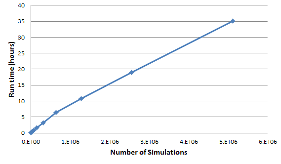
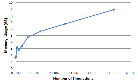
To evaluate how radar run-time and memory usage increases as the number of simulation, $N$, increases, we have generated a synthetic model whose characteristics are similar to that of the emergency response system, i.e. it contains 2 objectives, 10 decisions, 3 options per decisions, and no decision dependencies. We have then measured the running times and memory consumption of analysing this model when doubling $N$ 10 times from $10^{4}$ to $512\times 10^{4}$. The results are shown in Figure 1. They indicate that the running time and memory usage increase linearly with $N$ as expected from the theoretical complexity analysis.

Figure 1: Total run-time (left) and memory usage (right) measured for doubling the number of simulations, $N$, from $10^{4}$ to $512\times 10^{4}$.

RQ2: What is RADAR’s scalability with respect to design space size

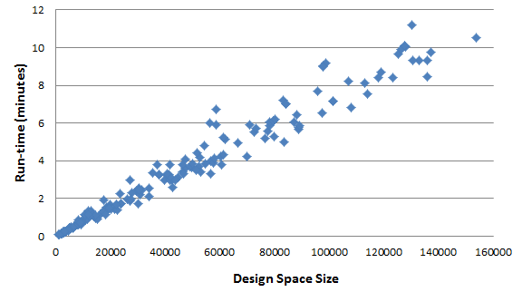
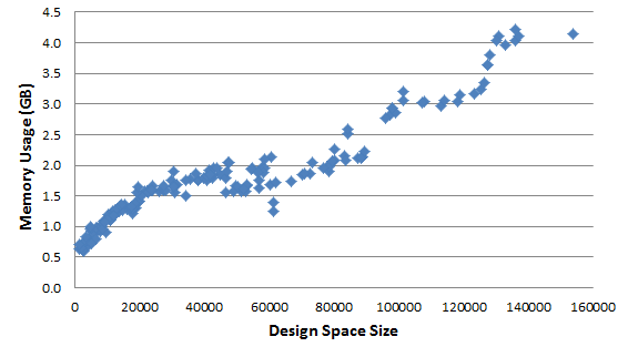
To evaluate how radar run-time and memory usage increases when the design space size increases, we have generated synthetic models by incrementally increasing the number of decisions and options per decisions until the resulting models could no longer be analysed in less than an hour. All models generated have 2 objectives and at least 100 model variables. The simulations are performed with $N=10^{4}$.

Figure 2 shows the result of this experiment. The largest model radar was able to evaluate in less than one hour models has a design space of up to 153,751 solutions and includes 11 decisions with 7 options per decision. The figure also show that, as expected from the theoretical analysis, the run-time and memory usage increase roughly linearly with the size of the design space.

Figure 2: Total run-time (left) and memory usage (right) measured for 180 radar models with different design space size.

RQ3: What is RADAR’s scalability with respect to the number of objectives

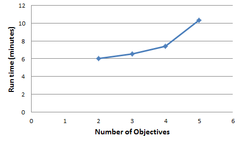
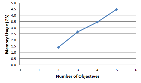
To evaluate how radar run-time and memory usage increases when the number of objectives increases, we have generated synthetic models with 10 decisions, 3 options per decisions, and incrementally increased the number of objectives from 2 to 5 until the resulting models could no longer be analysed in less than an hour. The synthetic models generated do not have decision dependencies. The size of their design space is thus $3^{10}=59,049$.

Figure 3 shows that on our synthetic models the run-time and memory usage increase roughly linearly with the number of objectives, as expected from the theoretical complexity analysis.

Figure 3: Total run-time (left) and memory usage (right) measured for 2,3,4 and 5 objectives.

RQ4: What is the time spent and memory consumed by each analysis step

For each synthetic model generated in the experiment to answer RQ2, we measured the fraction of time spent and memory used in each of the four analysis step: generating the design space, simulating the design space, shortlisting the Pareto-optimal solutions, and computing expected information value. Table II shows the average fraction of time for each analysis step over all synthetic models analysed in answer to RQ2 and RQ3. The table shows that the simulation of all solutions takes the largest portion of time (100%) and memory consumption (96%).

Algorithm Step	Average % Total Time	Average % Memory Usage
Generating the design space	0	0
Simulating all solutions in the design space	100	96
Shortlisting the Pareto-optimal solutions	0	1
Computing expected information value over the shortlisted solutions	0	3

TABLE II: Real world radar applications and their problem sizes.

III Conclusion

We have shown both theoretically and empirically that radar’s running time and memory usage increase linearly with the number of simulations, number of objectives and size of the design space. We also observed that radar’s running time is almost entirely consumed by the exhaustive simulation of the design space.

The design space size is the critical factor limiting the scalability of radar’s exhaustive simulation of the design space. Without decisions dependencies, the design space size increases exponentially with the number of decisions. This severely limits the class of decision problems radar can currently analyse. As a rule-of-thumb, radar’s exhaustive search strategy would struggle solving problems with more than 10 independent decisions with around 3 options per decisions.

Solving problems with larger design spaces will require adopting heuristic search-based approaches that can return good approximations of the set of Pareto-optimal solutions by exploring only small portions of the design space [5]. We intend to implement such search-based approach in the near future.

We are currently working on extending radar’s modelling language and analysis technique to deal with decision problems with non-mutually exclusive decisions. Such decisions problems have much larger design spaces than the ones we have encountered so far and will require an appropriate heuristic search strategy.

References

- [1] S. Busari and E. Letier, “Radar: A lightweight tool for requirements and architecture decision analysis,” in 39th International Conference on Software Engineering (ICSE 2017), 2017.
- [2] H.-T. Kung, F. Luccio, and F. P. Preparata, “On finding the maxima of a set of vectors,” Journal of the ACM (JACM), vol. 22, no. 4, pp. 469–476, 1975.
- [3] E. Letier, D. Stefan, and E. T. Barr, “Uncertainty, risk, and information value in software requirements and architecture,” in 36th International Conference on Software Engineering (ICSE 2014), 2014, pp. 883–894.
- [4] M. Sadatsafavi, N. Bansback, Z. Zafari, M. Najafzadeh, and C. Marra, “Need for speed: an efficient algorithm for calculation of single-parameter expected value of partial perfect information,” Value in Health, 2013.
- [5] M. Harman, S. A. Mansouri, and Y. Zhang, “Search-based software engineering: Trends, techniques and applications,” ACM Computing Surveys (CSUR), vol. 45, no. 1, p. 11, 2012.