Bayesian Multiscale Finite Element Methods. Modeling missing subgrid information probabilistically

Abstract

In this paper, we develop a Bayesian multiscale approach based on a multiscale finite element method. Because of scale disparity in many multiscale applications, computational models can not resolve all scales. Various subgrid models are proposed to represent un-resolved scales. Here, we consider a probabilistic approach for modeling un-resolved scales using the Multiscale Finite Element Method (cf., [1, 2]). By representing dominant modes using the Generalized Multiscale Finite Element, we propose a Bayesian framework, which provides multiple inexpensive (computable) solutions for a deterministic problem. These approximate probabilistic solutions may not be very close to the exact solutions and, thus, many realizations are needed. In this way, we obtain a rigorous probabilistic description of approximate solutions. In the paper, we consider parabolic and wave equations in heterogeneous media. In each time interval, the domain is divided into subregions. Using residual information, we design appropriate prior and posterior distributions. The likelihood consists of the residual minimization. To sample from the resulting posterior distribution, we consider several sampling strategies. The sampling involves identifying important regions and important degrees of freedom beyond permanent basis functions, which are used in residual computation. Numerical results are presented. We consider two sampling algorithms. The first algorithm uses sequential sampling and is inexpensive. In the second algorithm, we perform full sampling using the Gibbs sampling algorithm, which is more accurate compared to the sequential sampling. The main novel ingredients of our approach consist of: defining appropriate permanent basis functions and the corresponding residual; setting up a proper posterior distribution; and sampling the posteriors.

1 Introduction

Many problems in application domains have multiple scales. The scales in space and time are dominant in these applications that arise in porous media, material sciences and so on. Detailed descriptions at the finest scales often include uncertainties due to missing information. Moreover, there is often limited information about the solution available. For this reason, it is desirable to compute solutions within a probabilistic setup and estimate associated uncertainties, which is an objective of this paper.

One of the challenges in the computation of multiscale problems is the resolution of finest scales. Due to the grid resolution, one can not afford many degrees of freedom in each computational grid. Subgrid information are often modeled stochastically even for deterministic problems. For example, a typical approach for modeling subgrid information uses Representative Volume Element (RVE) to compute macroscopic quantities. However, because of uncertainties in RVE sizes and boundary conditions, the macroscopic parameters can not be modeled deterministically. It is advantageous in this and other multiscale applications to use probabilistic approaches to compute the solution. In this paper, our goal is to propose a novel modeling approach for missing subgrid information by setting up a Bayesian formulation.

The reduced-order modeling approaches have been commonly used in solving multiscale problems. These approaches include homogenization and numerical homogenization methods [3, 4, 5, 6, 7, 8, 9, 10], multiscale methods [5, 11, 12, 13, 14, 6, 15, 16, 17, 18, 19, 20, 21, 22], and so on. In homogenization and numerical homogenization approaches, the macroscopic information is computed using RVE simulations. In these approaches, the sizes of RVEs and limited number of local information can be insufficient to compute the solution accurately. In multiscale finite element methods, in particularly in Generalized Multiscale Finite Element Method (GMsFEM), multiscale basis functions are computed to systematically take into account missing subgrid information. In these approaches, the missing subgrid information is represented in the form of local multiscale basis functions. Using a few initial (dominant) basis functions, the error can be reduced substantially. The multiscale basis functions are computed under some assumptions. Our objective is to propose a Bayesian formulation, which can allow computing the multiscale solution and associated uncertainties with a few basis functions and stochastically representing the missing information.

The probabilistic approaches are important for problems when one has limited information about the solution. For example, it is common to measure the solution or averages at some locations with some precisions. In this case, to impose the constraint on the solution at some time instants, one can easily use additional constraints in the Bayesian framework by including additional multiplicative factors. Furthermore, one can include uncertainties in the media properties in the Bayesian framework and compute the solution and the uncertainties associated with the solution and the variations of the field parameters. Bayesian approaches for forward and inverse problems have been developed in many previous papers (e.g., [23, 24, 25, 26, 27]). Our approach shares some similarities with [28], though in our paper, we seek multiscale basis functions in a given set of basis functions.

Our approach starts with the Generalized Multiscale Finite Element framework. The GMsFEM was first presented in [29] and later investigated in several other papers (e.g., [30, 31, 32, 33, 34, 35, 36, 37, 38]). It is a generalization of the MsFEM and defines appropriate local snapshots and local spectral decompositions. This approach adds local degrees of freedom as needed and provides numerical macroscopic equations for problems without scale separation and identifies important features for multiscale problems. Because of the local nature of proposed multiscale model reduction, the degrees of freedom can be added adaptively based on error estimators. However, due to the computational cost, one often uses fewer basis functions. This can result to discretization errors, which we would like to represent in a Bayesian framework.

We consider the time-dependent equations

$${\partial u\over\partial t}=\mathcal{L}(\kappa(x,t),u,\nabla u),$$

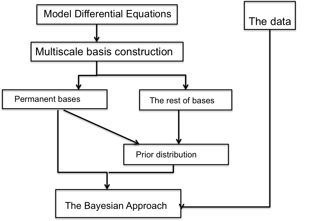
where $\kappa(x,t)$ is a heterogeneous space-time function and $\mathcal{L}$ is a differential operator. Our approach starts with constructing multiscale basis functions and uses a few basis functions as permanent basis functions (see Figure 1). It is known that these basis functions can provide a solution approximation. Additional basis functions are selected stochastically using the residual information. These basis functions are selected conditioned to the selection of subregions, which is based on the distribution of local residuals. The latter is used as a prior distribution.

To setup the posterior distribution, we start with an approximate solution computed with a few permanent basis functions and compute the corresponding residual. Using the residual information at the current time, we define a prior distributions for the basis selection. The likelihood includes the residual, which is minimized. We discuss several choices for the posterior distributions and two sampling algorithms. The first sampling algorithm is a sequential sampling and uses the prior distributions based on the residual to select the realizations of the solution. The second sampling algorithm, full sampling, seeks basis functions and the solution that can provided a desired error distribution. We note that a general flexibility of our proposed framework allows implementing various solution strategies and incorporating the data. In our approach, we do not seek ‘”very close” approximations of the solutions; but rather look for many approximate solutions. Below, we summarize our algorithm (see Figure 1):

• compute multiscale basis functions and identify permanent basis functions and “the rest” of basis functions;

• use the residual to compute prior distribution for “the rest” basis functions;

• setup a posterior, which includes the residual minimization and the data;

• sample the posterior distribution.

We present numerical results for parabolic and wave equations. Our numerical results study probabilistic approximations of the solution. We show that the full sampling provides better accuracy at a higher computational cost. The number of multiscale basis functions in full sampling depends on the threshold in the posterior and this is studied in the paper. The main novel ingredients of our approach are (1) defining appropriate permanent basis functions and corresponding residuals for priors; (2) setting up a proper posterior distribution, the likelihood, and the prior distribution; and (3) sampling methods, which explore these posterior distributions.

The paper is organized as follows. In Section 2, we present a general problem setup and motivation. Section 3 is devoted to our Bayesian algorithm. In this section, we describe some basic ingredients of our algorithm and setup the posterior distribution. In Section 4, we present numerical results for parabolic and wave equations.

Figure 1: Outline of the algorithm.

2 Problem setup, preliminaries, and motivation

We consider the forward model

$${\partial u\over\partial t}=\mathcal{L}(\kappa(x,t),u,\nabla u),$$ (1)

where $\mathcal{L}$ is a multiscale differential operator. For example, $\mathcal{L}(\kappa(x),u,\nabla u)=\text{div}(\kappa(x,t)\nabla u)$ or higher order differential operator, where $\kappa(x,t)$ is highly oscillatory coefficients.

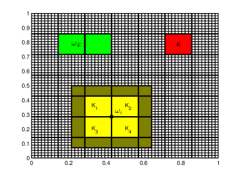
We consider solving (1) on a coarse grid (see Figure 2 for the illustration). Previous approaches construct multiscale basis functions on the coarse grid block to represent important degrees of freedom. However, the missing degrees of freedom are not modeled and the construction of basis functions often rely on some assumptions. In this paper, we use a Bayesian framework and develop a novel multiscale approach.

2.1 Computational grid. Description of coarse and fine grids

We introduce the notation for the coarse and fine grid. Computations are done on a coarse grid, where fewer basis functions are used. The computational domain is denoted by $\Omega$, which is partitioned by a coarse grid $\mathcal{T}^{H}$. The coarse grids contain multiscale features of the problem and require many degrees of freedom for modeling. We denote by $N_{c}$, the number of nodes in the coarse grid and by $N_{e}$ be the number of coarse edges. $K$ is a generic coarse element in $\mathcal{T}^{H}$. Multiscale basis functions are computed on a refinement of $\mathcal{T}^{H}$, called a fine grid $\mathcal{T}^{h}$, with mesh size $h>0$. The fine grid resolves multiscale features of the problem.

Figure 2: Illustration of fine grid, coarse grid, coarse neighborhood and oversampled domain.

2.2 General idea of multiscale basis construction

We discuss some general ideas of multiscale basis construction, which allows building basis functions to approximate some important features of the solution. We will focus on Generalized Multiscale Finite Element Method (GMsFEM). First, we discuss a variational formulation and then discuss the basis constructions. Some of the technical details about basis constriction are presented in Appendix B.

2.3 Variational formulation

The variational form reduces the PDE system into a system of linear equation. The dimension of the system is proportional to the number of basis. For very high dimensional system, as those considered in the paper, this leads to very large computational problems. We propose a Bayesian basis selection technique. This approach uses smaller number of basis on space-time grids in capturing the unresolved scale through stochastic approach. Typical subgrid basis functions representing the solutions over computational grids can not include all fine-grid information of the solution space. Some important subgrid information can be taken into account, while un-resolved scales and information can be modeled in a probabilistic fashion, as proposed in the paper.

As an example, we consider the parabolic differential equation (1) in a space-time domain $\Omega\times(0,T)$ and assume $u=0$ on $\partial\Omega\times(0,T)$ and $u(x,0)=\beta(x)$ in $\Omega$. We assume the source term is $f(x)$. We compute the solution $u_{H}$ in the time interval $(0,T)$. The solution space is denoted by $V_{H,\text{off}}^{(0,T)}$, which is a direct sum of the spaces only containing the functions defined on one single coarse time interval $(T_{n-1},T_{n})$, we can decompose the problem into a sequence of problems and find the solution $u_{H}$ in each time interval, denoted by $u_{H}^{n}$. The coarse space in each $(T_{n-1},T_{n})$ is constructed and denoted by $V_{H,\text{off}}^{(0,T)}=\oplus_{n=1}^{N}V_{H,\text{off}}^{(T_{n-1},T_{n})}$, where $V_{H,\text{off}}^{(T_{n-1},T_{n})}$ contains the functions having zero values in the time interval $(0,T)$ except $(T_{n-1},T_{n})$, namely $\forall v\in V_{H,\text{off}}^{(T_{n-1},T_{n})},$ $v(\cdot,t)=0\text{ for }t\in(0,T)\backslash(T_{n-1},T_{n})$.

The coarse-grid equation is to find

$${\color[rgb]{0,0,0}\begin{split}R^{n}_{v}(u_{H}^{n}(x,t),u_{H}^{n-1}(x,t))=\\ \int_{T_{n-1}}^{T_{n}}\int_{\Omega}\cfrac{\partial u_{H}^{n}}{\partial t}v+A(u_{H}^{n},u_{H}^{n-1},v)=0,\end{split}}$$ (2)

where $A$ corresponds to the PDE and its discretization and $v$ is the test functions. We will also investigate wave equations described in Section 4. In the paper, we will consider spatial formulations, but the method can be used for space-time method.

Example. In a continuous Galerkin formulation for parabolic equations with heterogeneous coefficients $\kappa$, we seek $u_{H}^{n}\in V_{H,\text{off}}^{(T_{n-1},T_{n})}$ (where $V_{H,\text{off}}^{(T_{n-1},T_{n})}$ will be defined later) satisfying

$$\begin{split}\int_{T_{n-1}}^{T_{n}}\int_{\Omega}\cfrac{\partial u_{H}^{n}}{\partial t}v+\int_{T_{n-1}}^{T_{n}}\int_{\Omega}\kappa\nabla u_{H}^{n}\cdot\nabla v+\int_{\Omega}u_{H}^{n}(x,T_{n-1}^{+})v(x,T_{n-1}^{+})\\ =\int_{T_{n-1}}^{T_{n}}\int_{\Omega}fv+\int_{\Omega}g_{H}^{n}(x)v(x,T_{n-1}^{+}),\end{split}$$ (3)

for all $v\in V_{H,\text{off}}^{(T_{n-1},T_{n})}$, where $g_{H}^{n}(\cdot)=\{u_{H}^{n-1}(\cdot,T_{n-1}^{-})\text{ for }n\geq 1;\beta(\cdot)\text{ for }n=0\}$, and $F(\alpha^{+})$ and $F(\alpha^{-})$ denote the right hand and left hand limits of $F$ at $\alpha$ respectively. Then, the solution $u_{H}$ of the problem in $(0,T)$ is the direct sum of all these $u_{H}^{n}$’s, that is $u_{H}=\oplus_{n=1}^{N}u_{H}^{n}$. In multiscale simulations, our objective is to define multiscale basis functions and minimize $R^{n}$ in the space of these basis functions. In our current approach, we would like to setup a Bayesian framework and sample a probability distribution related to $R^{n}$.

Remark 1.

We note that the residual can be written in a discrete form. In general, the discrete form is

$$R(u^{n+1}_{\text{d}isc},u^{n}_{\text{d}isc})=\Psi_{v}M_{\text{f}ine}\Phi_{u}u^{n+1}_{\text{d}isc}-\Psi_{v}M_{\text{f}ine}\Phi_{u}u^{n}_{\text{d}isc}+\Delta t\Psi_{v}A_{\text{f}ine}\Phi_{u}u^{n+1}_{\text{d}isc},$$

where $M_{\text{f}ine}$ and $A_{\text{f}ine}$ are fine-grid mass and stiffness matrices, $\Psi_{v}$ consists of the test space basis vectors, $\Phi_{u}$ consists of the trial basis vectors, and $u^{n}_{\text{d}isc}$ is a discretized solution at $n$th time step. The test functions are important for the stability in the proposed method. In the paper, we will mostly use the test spaces that correspond to snapshot spaces, but in general, one can use a test space consisting of all fine-grid functions.

Next, we discuss multiscale basis function construction procedure with details described in Appendix B.

2.4 Multiscale basis functions and snapshot spaces.

The main idea of a multiscale approach is to systematically select important degrees of freedom for the solution in each coarse block (see Figure 2 for coarse and fine grid illustration). For each coarse block $\omega_{i}$ (or $K$) and time interval $(T_{n-1},T_{n})$, we identify local multiscale basis functions $\phi_{j}^{n,\omega_{i}}$ ($j=1,...,N_{\omega_{i}}$) and seek the solution in the span of these basis functions. For problems with the scale separation, a limited number of degrees of freedom is sufficient. For more complicated heterogeneities as those that appear in many real-world applications, one needs a systematic approach to find the additional degrees of freedom. In each coarse grid (space-time), first, we construct the snapshot space, $V_{\text{snap}}^{n,\omega_{i}}=\text{span}\{\psi_{j}^{n,\omega_{i}}$}. The choice of the snapshot space depends on the global discretization and the particular application [18]. Each snapshot can be constructed, for example, using random boundary conditions or source terms [39], which allows avoiding the computations of all snapshot solutions. Details of snapshot spaces are presented in Appendix B.

Once we construct the snapshot space $V_{\text{snap}}^{n,\omega_{i}}$, we compute the offline space, which is a principal component subspace of the snapshot space. The offline space contains important degrees of freedom as first few basis functions. In this paper, our goal is to develop a Bayesian framework, which adaptively adds new basis functions to very few initial basis functions.

The offline space construction is discussed in Appendix B and in Section 4 for some examples. We denote the offline space by $V_{H,\text{off}}^{n,\omega_{i}}$ for a generic domain $\omega_{i}$ and time interval $(T_{n-1},T_{n})$ with elements of the space denoted $\phi_{l}^{n,\omega_{i}}$. The offline space is constructed by performing a spectral decomposition in the snapshot space. By selecting the dominant eigenvectors (corresponding to the smallest eigenvalues), we choose the elements of the offline space [18]. The choice of the spectral problem is important for the convergence and is derived from the analysis as it is described below. The convergence rate of the method is proportional to $1/\Lambda_{*}$. Here, $\Lambda_{*}$ is the smallest eigenvalue among all coarse blocks whose corresponding eigenvector is not included in the offline space. Our goal is to select the local spectral problem to remove as many small eigenvalues as possible so that we can obtain smaller dimensional coarse spaces to achieve a higher accuracy.

3 Bayesian formulation

We seek the solution in each coarse time interval $(T_{n-1},T_{n})$

$$u^{n}_{H}(x,t)=\sum_{i,j}\beta_{i,j}^{n}\ \phi_{i}^{n,\omega_{j}}(x,t),$$

where $\beta_{i,j}^{n}$’s are defined in each computational time interval and $\phi_{i}^{n,\omega_{j}}(x,t)$ are basis functions. We will choose $\phi_{i}^{n,\omega_{j}}$ to be time-independent, in general. in this paper.

For further description, we introduce some notations. First, we select some basis functions in each selected subdomain, which will be used as permanent multiscale basis functions. These are first dominant modes (typically a few basis functions) in each coarse domain and denoted by

$$\phi_{i}^{n,\omega_{j}}(x,t)\ -\ \text{permanent basis functions}.$$

Furthermore, we will select basis functions from the rest of the space, which we denote by

$$\phi_{i,+}^{n,\omega_{j}}(x,t)\ -\ \text{the rest of basis functions}$$

in order to distinguish from the first few basis functions. The solution is sought as

$$u^{n}_{H}(x,t)=\sum_{i,j}\beta_{i,j}^{n}\ \phi_{i}^{n,\omega_{j}}(x,t)+\sum_{i,j}\beta_{i,j,+}^{n}\ \phi_{i,+}^{n,\omega_{j}}(x,t).$$

“Fixed” multiscale solution with permanent basis functions. In our approaches, we will use “fixed” multiscale solution computed using permanent basis function. We denote this solution by

$$u^{n,\text{fix}}_{H}(x,t)=\sum_{i,j}\gamma_{i,j}^{n}\ \phi_{i}^{n,\omega_{j}}(x,t),$$ (4)

where $\gamma$’s are computed from

$$A(\gamma^{n})=R^{n,\text{fix}}_{v}(u_{H}^{n}(x,t),u_{H}^{n}(x,T_{n-1}^{+}),u_{H}^{n-1}(x,T_{n-1}^{-}))=0,$$

where $v$ are offline basis functions.

Next, we describe some general steps of our algorithms, which are used to define posterior functionals.

• Problem under consideration

  $${\partial u\over\partial t}=\mathcal{L}(u).$$ (5)

• We seek the solution in the time interval $(T_{n-1},T_{n})$, as

  $$u^{n}_{H}(x,t)=\sum_{i,j}\beta_{i,j}^{n}\ \phi_{i}^{n,\omega_{j}}(x,t)+\sum_{i,j}\beta_{i,j,+}^{n}\ \phi_{i,+}^{n,\omega_{j}}(x,t).$$

  Here, basis functions $\phi_{i}^{n,\omega_{j}}(x,t)$ are kept fixed and $\phi_{i,+}^{n,\omega_{j}}(x,t)$ are selected based on the indicator $\mathcal{I}$ for basis index and the indicator $\mathcal{J}$ for subdomains. The indicators are defined later and represent the indices of basis functions and subdomains that are selected in simulations.

• Denote the global residual at time $(T_{n-1},T_{n})$ by $\mathcal{R}^{n}$ and the residual for the subdomain $\omega_{j}$ by $\mathcal{R}^{n}_{\omega_{j}}$. We will consider several possible residuals: $R^{n,\text{fix}}_{v}(u_{H}^{n,\text{fix}}(x,t),u_{H}^{n,\text{fix}}(x,T_{n-1}^{+}),u_{H}^{n-1,\text{fix}}(x,T_{n-1}^{-}))$; and $R^{n}_{v}(u_{H}^{n}(x,t),u_{H}^{n}(x,T_{n-1}^{+}),u_{H}^{n-1}(x,T_{n-1}^{-}))$. In all cases, $v$ is assumed to be in a large dimensional snapshot space. $\mathcal{R}^{n}$ and $\mathcal{R}^{n}_{\omega_{j}}$ are vectors corresponding to these residuals.

• First, we select $N_{\omega}$ subdomains, where multiscale basis functions will be added. We denote by $\alpha^{\omega_{k}}=\|\mathcal{R}^{n}_{\omega_{k}}\|/\|\mathcal{R}^{n}\|$, where $\mathcal{R}^{n}$ is the global residual vector and $\mathcal{R}^{n}_{\omega_{k}}$ is the local residual vector in $\omega_{k}$ (as mentioned earlier). Furthermore, we denote by

  $$\widehat{\alpha}^{\omega_{k}}={{\alpha}^{\omega_{k}}\over\sum_{j}{\alpha}^{\omega_{j}}}N_{\omega},$$

  where $N_{\omega}$ is the desired number of average subregions that is the user’s choice and depends on available computer resources. With probability $\widehat{\alpha}^{\omega_{k}}\wedge 1$, we select the region $\omega_{k}$, i.e., $\mathcal{J}_{k}=1$ if the region is selected.

  Remark 2.

  We note that we can compute the residual only at few locations to evaluate the prior probability distributions.

• We use permanent basis functions $\phi_{i}^{n,\omega_{j}}$ in every region and select additional $N_{\text{basis}}$ basis functions (as above) using the residual. The number of basis, $N_{\text{basis}}$, is the user’s choice and depends on available computer resources. For each $\omega_{j}$, we compute the correlation coefficient

  $$\text{corrcoeff}(\mathcal{R}^{n}_{\omega_{j}},\phi_{k,+}^{n,\omega_{j}})=\alpha_{k,+}.$$

  We normalize these $\alpha_{k,+}$ (we keep the same notation as for subdomain indices) so that on average we have $N_{\text{basis}}$ basis functions.

  $$\widehat{\alpha}_{k,+}={\alpha_{k,+}\over\sum\alpha_{i,+}}N_{\text{basis}}.$$

  I.e., in a prior distribution, we choose $k$th basis with probability $\widehat{\alpha}_{k,+}\wedge 1$. Since $\widehat{\alpha}_{k,+}$ are used as a prior information, one can use the residual at a few fixed locations or approximate residuals to compute this prior.

• We will consider several posteriors.

  Posterior around fixed solution. In this case, we will use the solution $[0,T]$ computed using permanent basis to sample realizations. We sample

  $$\begin{split}P(\beta_{+}^{1:N_{T}},\mathcal{I}^{1:N_{T}},\mathcal{J}^{1:N_{T}}|u^{1:N_{T},\text{fix}}_{H}(x,t))\sim P(u^{1:N_{T},\text{fix}}_{H}(x,t)|\beta_{+}^{1:N_{T}}(\mathcal{I}^{1:N_{T}},\mathcal{J}^{1:N_{T}}))\\ \pi(\beta_{+}^{1:N_{T}}|\mathcal{I}^{1:N_{T}},\mathcal{J}^{1:N_{T}})\pi(\mathcal{I}^{1:N_{T}},\mathcal{J}^{1:N_{T}}),\end{split}$$ (6)

  where superscript $1:N_{T}$ refers to the whole time interval of the sampled quantities,

  $$\begin{split}P(u^{1:N_{T},\text{fix}}_{H}(x,t)|\beta_{+}^{1:N_{T}}(\mathcal{I}^{1:N_{T}},\mathcal{J}^{1:N_{T}}))\sim\exp\left(-{\|R^{n,\text{fix}}_{v}\|^{2}\over\sigma_{L}^{2}}\right)\end{split}$$ (7)

  and

  $$\pi(\beta_{+}^{1:N_{T}}|\mathcal{I}^{1:N_{T}},\mathcal{J}^{1:N_{T}})=\exp\left(-{\|\beta_{+}^{1:N_{T}}\|^{2}\over\sigma_{2}^{2}}\right)$$

  Here, $R^{n,\text{fix}}_{v}$ is the residual computed using $u^{1:N_{T},\text{fix}}_{H}(x,t)$, $\|\cdot\|$ is a discrete $l^{2}$ norm, and $\sigma_{L}$ represents the precision of the numerical approximation. Here, $\sigma_{2}$ is the variance for the prior and, in our numerical simulations, we ignore the prior for $\beta_{+}^{1:N_{T}}$, and so, one can assume that $\sigma_{2}$ is a large number. In fact, the posterior is computed around the residual corresponding to the fixed solution. This posterior will be used in the example for parabolic equations (Sections 4.1 and 4.2).

  Posterior around previous time. In the second case, we will sample at each time interval based on the previous time sampled solution. In this case, we re-compute the coefficients corresponding to fixed basis functions.

  $$\begin{split}P(\beta^{n+1},\mathcal{I}^{n+1},\mathcal{J}^{n+1}|u^{n}_{H}(x,t)))\sim P(u^{n}_{H}(x,t))|\beta^{n+1}(\mathcal{I}^{n+1},\mathcal{J}^{n+1}))\\ \pi(\beta^{n+1}|\mathcal{I}^{n+1},\mathcal{J}^{n+1})\pi(\mathcal{I}^{n+1},\mathcal{J}^{n+1})\end{split}$$ (8)

  $$\begin{split}P(u^{n}_{H}(x,t))|\beta^{n+1}(\mathcal{I}^{n+1},\mathcal{J}^{n+1}))\sim\exp\left(-{\|R^{n+1}_{v}\|^{2}\over\sigma_{L}^{2}}\right)\end{split}$$ (9)

  Here, $R^{n+1}_{v}$ is the residual computed using $u^{n}_{H}(x,t)$ as an initial condition and permanent basis functions in the current time interval $(T_{n},T_{n+1})$, $\|\cdot\|$ is a discrete $l^{2}$ norm, and, again, $\sigma_{L}$ represents the precision of the numerical approximation. In fact, the posterior is computed around the residual corresponding to the solution at previous time step. This posterior will be used in the example for wave equations (Sections 4.3).

  Posterior using fixed and previous time solutions. One can condition the multiscale solution at the fixed solution $u^{1:N_{T},\text{fix}}_{H}(x,t)$ and $u^{n}_{H}(x,t)$. In this case, one can seek a posterior distribution for

  $$P(u^{n+1}_{H}(x,t)|u^{n}_{H}(x,t),u^{1:N_{T},\text{fix}}_{H}(x,t)).$$

  Other more general posteriors can also be setup.

3.1 Sampling from the posterior distribution

We will consider two sampling algorithms. In the first sampling algorithm (we call “sequential sampling”), we will use samples from the prior distribution and use them to obtain samples of $\beta$’s. In this process, in the first step, we sample $\mathcal{I}$ and $\mathcal{J}$ from the prior based on the residual and use them to compute the samples of $\beta$. In our numerical experiments, we will show the results for $E(\beta^{n+1}|\mathcal{I}^{n+1},\mathcal{J}^{n+1})$.

In the second algorithm, we will perform full posterior sampling (we call “full sampling”), where we will sample both the indices ($\mathcal{I}$, $\mathcal{J}$) and the coefficients ($\beta$). In this case, we will use Gibbs sampling [40, 41], though one can also design efficient sampling algorithms based on Markov chain Monte Carlo methods [40, 41]. In Gibbs sampling, we will compute the probabilities $\hat{\pi}_{i}$ for each additional basis function as

$$\frac{\hat{\pi}^{n+1}_{i+}}{1-\hat{\pi}^{n+1}_{i+}}=\frac{\hat{\alpha}^{n+1}_{i+}}{1-\hat{\alpha}^{n+1}_{i+}}*\mathcal{F},$$

where $\mathcal{F}$ is a multiplication factor that depends how much a change in one basis function (i.e., adding a basis function) will affect the residual change. This factor also depends on the model size. To penalize adding linearly dependent basis functions, we modify the prior distribution $\pi(\mathcal{I},\mathcal{J})$ with a multiplicative constant, which takes into account the linear dependency factor. This multiplicative factor is a product of the singular values of the matrix consisting of an inner product of basis functions such that the resulting $\sigma^{2}\log(\mathcal{F})$ reduces to the difference between two residuals. Note that in this step, it is important to have a computable residual.

3.2 Dynamic data

In our proposed approach, the threshold $\sigma_{L}$ (e.g., in (7)) represents the accuracy of our approximation. If we let $\sigma_{L}$ approach to zero, our sampling will increase the number of basis functions and the solution will converge to the fine-grid solution. However, the main idea of our approach is to allow less accurate solutions. The threshold in (7) can depend on the additional dynamic data. We can add the time-dependent data by including additional terms in the posterior distribution. For example, if we obtain the measurements of the solution at some locations, this can be added as an additional multiplicative term in the posterior (e.g., in (6)) in the form of

$$\exp\left(-{\|\mathcal{D}(u_{H}^{n+1})-\mathcal{D}_{obs}\|^{2}\over\sigma_{d}^{2}}\right),$$

where $\mathcal{D}(u_{H}^{n+1})$ is the observation that depends on the solution and $\mathcal{D}_{obs}$ is the associated observed data. We note that $\sigma_{d}$ is a factor in choosing the accuracy of our approximation. For example, if the measurement accuracy $\sigma_{d}$ is large, one can choose $\sigma_{L}$ also to be large.

4 Numerical examples

In our numerical results, we will compare two sampling approaches. In the first approach, the basis functions will be selected from the prior distribution and we will show the mean of the conditional distributions. In the second approach, we will apply Gibbs sampling to sample the realizations. Our numerical results will show that both approaches provide a good accuracy (in a statistical sense) and the Gibbs sampling is more accurate compared when sampling from the prior distribution. Moreover, we observe a fast convergence when using Gibbs sampling.

We will consider several problems. In the first example, we consider a parabolic problem and two different discretizations. In the second example, we will consider the wave equations. In each example, we will specify the residual that is used in the sampling. We note that it is important that this residual provides a good stability for the solution.

4.1 Mixed formulation for parabolic equations

For the mixed GMsFEM, the support of multiscale basis functions are $\omega_{E}$, which are the two coarse elements sharing a common edge $E$ (see [42] for details). In particular, we denote $\mathcal{E}^{H}$ as the set of all coarse grid edges and let $N_{e}$ be the total number of coarse grid edges. The coarse grid neighborhood $\omega_{E}$ of a face $E\in\mathcal{E}^{H}$ is defined as

$$\omega_{E}=\bigcup\{K\in\mathcal{T}^{H}:E\in\partial K\},\quad i=1,2,\cdots,N_{e},$$

which is a union of two coarse grid blocks if $E_{i}$ is an interior edge (face) For a coarse edge $E_{i}$, we write $\omega_{E_{i}}=\omega_{i}$ to unify the notations. Multiscale basis functions are constructed using local snapshot spaces and local spectral problems (see [42] for details). Here, we will discuss the residual which is used in our Bayesian Multiscale Method.

We denote $Q_{H,\text{off}}$ as the space of functions which are piecewise constant on each coarse block. We will use this space to approximate the pressure $u$. For approximating the velocity $\mathcal{V}=-\kappa\nabla u$, we will construct a multiscale space $V_{H,\text{off}}$ for the velocity by following the general framework of the GMsFEM. Next, we use the spaces $Q_{H,\text{off}},V_{H,\text{off}}$ to solve the problem: to find $u^{n+1}_{H}\in Q_{H,\text{off}}$ and $\mathcal{V}^{n+1}_{H}\in V_{H,\text{off}}$ such that

$$\begin{split}\int_{\Omega}\kappa^{-1}\mathcal{V}^{n+1}_{H}\cdot w-\int_{\Omega}\mbox{div}(w)u^{n+1}_{H}=0,\ \forall w\in V_{H,\text{off}},\\ \int_{\Omega}(\cfrac{u^{n+1}_{H}-u^{n}_{H}}{\Delta t}+\mbox{div}(\mathcal{V}^{n+1}_{H}))q=\int_{\Omega}f^{n+1}q,\ \forall q\in Q_{H,\text{off}}.\end{split}$$ (10)

The residual is defined as

$$R_{w}^{n}(\mathcal{V}^{n+1}_{H,+},\mathcal{V}^{n+1,\text{fix}}_{H},u^{n+1,\text{fix}}_{H})=\int_{\Omega}\kappa^{-1}(\mathcal{V}^{n+1}_{H,+}+\mathcal{V}^{n+1,\text{fix}}_{H})\cdot w-\int_{\Omega}\mbox{div}(w)u^{n+1,\text{fix}}_{H}.$$

Denote $\mathcal{R}^{n}$ to be corresponding coordinates and use discrete $l^{2}$ norm as the residual norm.

Figure 3: The permeability field $\kappa$.

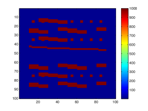
Next, we will present an example. We use the permeability field $\kappa$ shown in Figure 3 and the contrast of the permeability field $\cfrac{\max{\kappa}}{\min{\kappa}}$ is increasing as $\cfrac{\max{\kappa}}{\min{\kappa}}=1000e^{250t}$. In this example, we find the distribution of the solution at two different time instants $T=0.01$ and $T=0.02$. The fine grid is $100\times 100$ and the coarse grid is $10\times 10$. We use only one permanent basis function per edge to compute “fixed” solution and use our Bayesian framework to seek additional basis functions by solving small global problems. In our approach, first using the global residual we define local regions, where multiscale basis functions are added. We choose $\sigma_{L}=1e-3$. In our example, we fixed these local regions in each time step and choose $25$% and $55$% of the total coarse edges for the first and second time step, where the residual is larger than a certain threshold. In these coarse blocks, we apply both sequential sampling and full sampling algorithms.

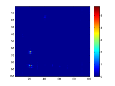
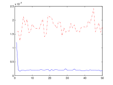
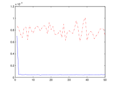
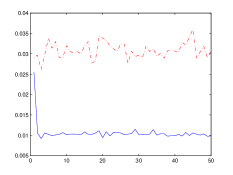
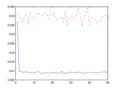
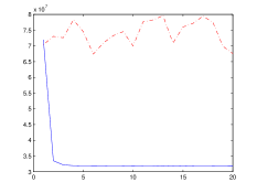
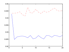
In Figure 4, we depict the mean solution using the sequential sampling algorithm and full sampling algorithms. The errors for the mean at $T=0.02$ are $3.02\%$ for the sequential sampling and $0.79\%$ for full sampling. We note that full sampling provides a better result. We observe similar results for $x_{2}$ component of the solution. We depict the standard deviation of the solution at each pixel in Figure 5. We observe that the true solution falls within the limits of the mean and the standard deviations. Next, we show the results across several samples. For the sequential sampling, we use $20$ realizations and show both residuals and the errors in Figure 6 and 7. The error is computed as a difference between the solution and the snapshot solution using the snapshot vectors in the elements, where the basis functions are updated. From these figures, we observe that the residuals and errors are smaller for full sampling compared to sequential sampling. Moreover, Gibbs sampling stabilizes in a few iterations, which shows a fast numerical convergence.

Figure 4: Plots of $x_{1}$-component of the numerical velocity $\mathcal{V}$ at $T=0.02$: reference solution (left), mean of sequential sampling (middle), mean of full sampling (right).

Figure 5: Plots of sample standard deviation of $x_{1}$-component of the velocity at $T=0.02$: sequential sampling (left), full sampling (right).

Figure 6: Residual vs. samples for sequential sampling (red dotted line) and full sampling (blue solid line): at time $T=0.01$ (left), at time $T=0.02$ (right).

Figure 7: $L^{2}$ vs. sample using sequential sampling (red dotted line) and full sampling (blue solid line): at time $T=0.01$ (left), at time $T=0.02$ (right).

Figure 8: History of occurrence probability against basis functions using sequential sampling (red dotted line) and full sampling (blue solid line): at time $T=0.01$ (left), at time $T=0.02$ (right).

Figure 9: History of number of basis functions against sampling process using sequential sampling (red dotted line) and full sampling (blue solid line): at time $T=0.01$ (left), at time $T=0.02$ (right).

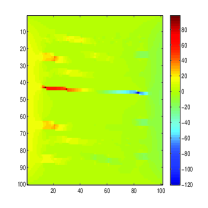
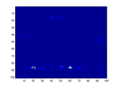
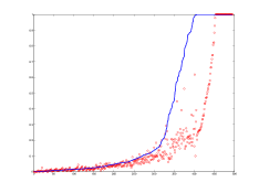
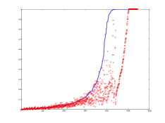
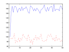
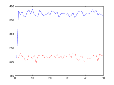
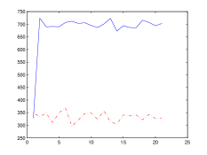
In Figure 8, we depict the frequency of the basis functions in both sequential and full sampling. We have enumarated the basis functions such that the frequency in full sampling is increasing. We observe from this figure that the sequential sampling has a similar trend and we have found the correlation in the frequencies between full sampling and partial sampling to be $0.7$. The shift in sequential sampling is due to the fact that fewer basis are used in this sampling. We plot the total number of basis functions in Figure 9. We observe from this figure that the full sampling requires more basis functions compared to the sequential sampling. Moreover, the number of basis functions in full sampling stabilizes around a certain value, which depends on $\sigma_{L}$ (the precision of the residual in (7)).

4.2 Continuous Galerkin formulation for parabolic equations

In this section, we present the Bayesian approach for the continuous Galerkin formulation. Multiscale basis functions are obtained from eigenfunctions in the local snapshot space with small eigenvalues in an appropriate local spectral eigenvalue problem (see [18] for details). We denote the space of multiscale basis functions by $V_{H,\text{off}}$, in which we seek numerical approximations for the problem: find $u_{H}^{n+1}\in V_{H,\text{off}}$ such that

$$\int_{\Omega}\cfrac{u^{n+1}_{H}-u^{n}_{H}}{\Delta t}\,v+\int_{\Omega}\kappa\nabla u^{n+1}_{H}\cdot\nabla v=\int_{\Omega}f^{n+1}v,\ \forall v\in V_{H,\text{off}}.$$ (11)

The residual is defined as

$$\begin{split}R^{n}_{v}(u_{+}^{n+1},u_{\text{fixed}}^{n+1},u_{\text{fixed}}^{n})&=\int_{\Omega}f^{n+1}v-\int_{\Omega}\cfrac{u^{n+1}_{+}+u_{\text{fixed}}^{n+1}-u_{\text{fixed}}^{n}}{\Delta t}\,v\\ &\quad\quad+\int_{\Omega}\kappa\nabla(u^{n+1}_{+}+u_{\text{fixed}}^{n+1})\cdot\nabla v.\end{split}$$ (12)

We use the permeability field $\kappa$ as in Figure 3. We will compare the solutions at two different time instants $T=0.01$ and $T=0.02$. The fine grid is $100\times 100$ and the coarse grid is $10\times 10$. We use $2$ permanent basis functions per coarse neighborhood to compute “fixed” solution and use our Bayesian framework to seek additional basis functions by solving small global problems. In this example, we select $30\%$ of the total local regions at which residual is the largest and multiscale basis functions are added. In these coarse blocks, we apply both sequential sampling and full sampling.

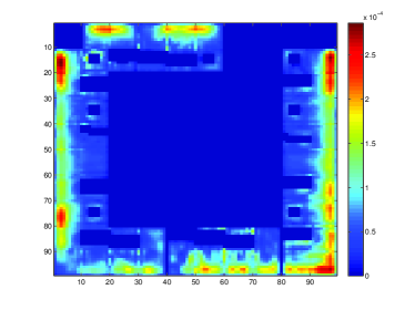
Figure 10 shows the reference solution and the sample mean at $T=0.2$. The $L^{2}$ error for the mean at $T=0.02$ is $0.92\%$ in the full sampling method, lower than $2.24\%$ in the sequential sampling method. Figure 11 shows the pixel-wise standard deviation of the samples. It can be seen that the deviation is smaller in full sampling.

Figure 10: Plots of the reference solution (left) and sample mean of numerical solution at $T=0.02$: sequential sampling (middle), full sampling (right).

Figure 11: Plots of sample standard deviation of numerical solution at $T=0.02$: sequential sampling (left), full sampling (right).

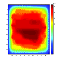
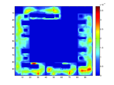
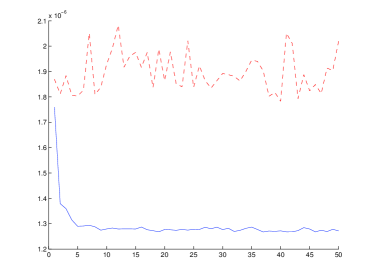
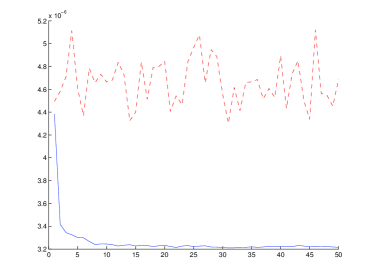
In Figures 12 and 13, the residual and $L^{2}$ errors are plotted for both sequential and full sampling. We observe that the errors and the residual in full sampling decrease and stabilize in a few iterations. Moreover, the full sampling gives more accurate solutions associated with our error threshold in the residual. In Figure 14, we plot the frequency of the basis functions vs. sample that appear in full and sequential sampling. The correlation of the frequencies is $0.87$, which indicates that we have a good prior model based on the residual. Finally, in Figure 15, we show the full number of basis functions. As we observe that the number of basis functions in full sampling approaches to a steady state, which depends on the error threshold $\sigma_{L}$ (see (7)).

Figure 12: Residual vs sample using sequential sampling (red dotted line) and full sampling (blue solid line): at time $T=0.01$ (left), at time $T=0.02$ (right).

Figure 13: $L^{2}$ error vs sample using sequential sampling (red dotted line) and full sampling (blue solid line): at time $T=0.01$ (left), at time $T=0.02$ (right).

Figure 14: History of occurrence probability against basis functions using sequential sampling (red dotted line) and full sampling (blue solid line): at time $T=0.01$ (left), at time $T=0.02$ (right).

Figure 15: History of number of basis functions against sampling process using sequential sampling (red dotted line) and full sampling (blue solid line): at time $T=0.01$ (left), at time $T=0.02$ (right).

4.3 Wave equation

In this section, we present an application of our approach to wave equations. Multiscale basis function construction follows to a similar procedure described in Appendix B with some slight modifications, see [43] for details. Here, we describe the residual that is used in our Bayesian framework.

We will use IPDG method with multiscale basis functions to solve the following wave equation,

$$\frac{\partial^{2}u}{\partial t^{2}}=\nabla\cdot(a\nabla u)+f\quad\quad\mbox{ in }\quad\Omega\times[0,T].$$ (13)

The IPDG method is to find $u_{H}$ such that

$$\int_{\Omega}\frac{\partial^{2}u_{H}}{\partial t^{2}}\,v+a_{DG}(u_{H},v)=\int_{\Omega}f\,v,\quad\quad\forall\,v\in V_{H},$$ (14)

where the bilinear form $a_{DG}(u,v)$ is defined by

$$a_{DG}(u,v) = \sum_{K\in\mathcal{T}^{H}}\int_{K}a\nabla u\cdot\nabla v+\sum_{e\in\mathcal{E}^{H}}(-\int_{e}\{a\nabla u\cdot n\}_{e}\,[v]_{e}$$

$$-\int_{e}\{a\nabla v\cdot n\}_{e}\,[u]_{e}+\cfrac{\gamma}{h}\int_{e}a[u]_{e}\,[v]_{e}),$$

with $\gamma>0$ is a penalty parameter and $n$ denotes the unit normal vector on $e$. Let $\Delta t>0$ be the time step size. We will consider the classical second order central finite difference method for time discretization, i.e., we find $u^{n+1}_{H}$ such that

$$\int_{\Omega}\frac{u^{n+1}_{H}-2u^{n}_{H}+u^{n-1}_{H}}{\Delta t^{2}}v+a_{DG}(u^{n}_{H},v)=\int_{\Omega}f^{n}\,v\quad\quad\forall\,v\in V_{H}.$$

We compute the solution $u_{H}^{n+1}$ at $n+1$ th time level, starting with the offline space. In each coarse element $K\in\mathcal{T}^{H}$, we define the local residual operator, $R_{v}^{n}$, as

$$R_{v}^{n}(u^{n+1}_{H},u^{n}_{H},u^{n-1}_{H})=(\cfrac{u_{H}^{n+1}-2u_{H}^{n}+u_{H}^{n-1}}{\Delta t^{2}},v)+a_{DG}(u_{H}^{n},v)-(f^{n},v),$$

and the operator norm of local residual functional is defined by

$$\|\mathcal{R}_{K}^{n}\|=\sup_{v\in V_{h}(K)}\cfrac{|R_{v}^{n}|}{\|v\|_{L^{2}(K)}}.$$

Figure 16: The medium $a$.

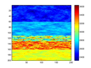
We use the medium $a$ shown in Figure 16. In this example, we find the distribution of the solution at the time instants $T=0.4$. The fine grid is $200\times 200$ and the coarse grid is $20\times 20$. We use one permanent basis function per edge to compute “fixed” solution and use our Bayesian framework to seek additional basis functions by solving small global problems. In this approach, we use previous time solution in the posterior. In our approach, using the global residual, some local regions ($17$ % of total coarse regions) are defined, where multiscale basis functions are added. In these coarse blocks, we apply both sequential sampling and full sampling algorithms.

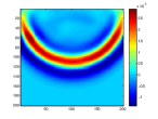
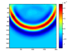
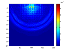
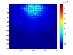
In Figure 17, we depict the mean solution using the sequential sampling algorithm and full sampling algorithms. The errors for the mean are $4.47\%$ for the sequential sampling and $2.67\%$ for full sampling. As before, the full sampling algorithm provides a more accurate result. We depict the standard deviation of the solution at each pixel in Figure 18. We observe that the true solution falls within the limits of the mean and the standard deviations. Next, we show the results across several samples. For the sequential sampling, we use $20$ realizations and show both residuals and the errors in Figure 19 and 20. The error is computed as a difference between the solution and the snapshot solution using the snapshot vectors in the elements, where the basis functions are updated. From these figures, we observe that the residuals and errors are smaller for full sampling compared to sequential sampling. Moreover, Gibbs sampling stabilizes in a few iterations. In Figure 21, we plot the total number of basis functions for samples. As we observe that the full sampling results to about $700$ additional basis functions (on average) for the entire domain. This number is affected by the error threshold $\sigma_{L}$ (see (7)) that we impose in the posterior distribution.

Figure 17: Numerical solution at $T=0.4$. Left: reference solution, Middle: mean solution for sequential sampling, Right: mean solution for full sampling.

Figure 18: Standard deviation of the solution. Left: sequential sampling, Right: full sampling

Figure 19: Residual vs sample using sequential sampling (red dotted line) and full sampling (blue solid line) at the final time.

Figure 20: $L^{2}$ error vs sample using sequential sampling (red dotted line) and full sampling (blue solid line) at the final time.

Figure 21: History of number of basis functions against sampling process using sequential sampling (red dotted line) and full sampling (blue solid line): at time T = 0.4.

5 Conclusions

In this paper, we propose a novel Bayesian Multiscale Finite Element approach. The main idea of the approach is to solve time-dependent problems, e.g., parabolic equations or wave equations, using multiscale basis functions in each coarse grid. It is known that [18] first few basis functions reduce the error substantially, while the “rest” of basis functions may reduce error significantly less. This is due to global effects. Various online approaches (e.g., [18] and the references therein) are proposed to remedy this situation. The online approaches are expensive as we need to compute new basis functions. In this paper, we propose a rigorous sampling for “rest” of basis functions, which allow computing multiple realizations of the solution and thus provide a probabilistic description for un-resolved scales. Our approaches are motivated by recent work [2], where the authors propose a probabilistic numerical method.

In the paper, we present a description of the method and sampling algorithms for un-resolved scales. Several posterior distributions are considered and two sampling mechanisms are studied. In both sampling methods, we use local residuals as a prior distributions for selecting multiscale basis functions. In the first approach, multiscale basis functions are selected from the prior distribution, while in the second approach, we present a full sampling using the Gibbs sampling. We show that the Gibbs sampling rapidly stabilizes at the steady state and provides a more accurate approximation at an additional cost. We consider several discretizations and applications to wave and parabolic equations. In general, the proposed method can be used to condition the solutions at measurement locations or computing solutions in stochastic environments. In this case, one can combine the precisions of the forward and inverse simulations in a unified way. This will be studied in our future work.

Appendix A Some Notations

• $\omega_{i}$ is a subdomain with a common vertex at $x_{i}$; $\omega_{E}$ is a subdomain with a common edge $E$; $K$ is a coarse-grid block

• $u_{H}$ is the coarse-grid multiscale solution; $u_{H}^{n}$ is the coarse-grid space-time multiscale solution defined on $(T_{n-1},T_{n})$

• $\psi_{i}^{\omega_{j}}$ - local snapshot solutions in the oversampled region $\omega_{j}$; $\phi_{i}^{\omega_{j}}$ - local offline basis in $\omega_{j}$

• $\phi_{i}^{n,\omega_{j}}$ - permanent (first few) local offline basis in $\omega_{j}$; $\phi_{i,+}^{n,\omega_{j}}$ - the rest of basis functions in $\omega_{j}$

• $u_{H}^{n,\text{fix}}$ is the solution in $(T_{n-1},T_{n})$ computed using permanent basis functions

• $R^{n,\text{fix}}_{v}(u_{H}^{n,\text{fix}}(x,t),u_{H}^{n,\text{fix}}(x,T_{n-1}))$ - the residual corresponding to fixed solution, $v$ is the test function

• $\mathcal{R}^{n}$ - the global residual vector; $\mathcal{R}^{n}_{\omega_{j}}$ - the local residual vector in $\omega_{j}$

• $V_{H,\text{off}}$ is the offline space in $\Omega$; $V_{H,\text{off}}^{\omega_{i}}$ is the offline space in $\omega_{i}$; $V_{H,\text{snap}}$ is the snapshot space in $\Omega$; $V_{H,\text{snap}}^{\omega_{i}}$ is the snapshot space in $\omega_{i}$

• $V_{H,\text{off}}^{(T_{1},T_{2})}$ is the offline space in $\Omega\times(T_{1},T_{2})$; $V_{H,\text{off}}^{\omega_{i},(T_{1},T_{2})}$ is the offline space in $\omega_{i}\times(T_{1},T_{2})$; $V_{H,\text{snap}}^{(T_{1},T_{2})}$ is the snapshot space in $\Omega\times(T_{1},T_{2})$; $V_{H,\text{snap}}^{\omega_{i},(T_{1},T_{2})}$ is the snapshot space in $\omega_{i}\times(T_{1},T_{2})$

Appendix B Space-time basis construction details

B.1 Snapshot space

Let $\omega$ be a coarse neighborhood in space. Coarse node index is omitted to simplify the notations. The construction of the offline basis functions in $(T_{n-1},T_{n})$ uses a snapshot space $V_{H,\text{snap}}^{\omega}$ (or $V_{H,\text{snap}}^{\omega,(T_{n-1},T_{n})}$). For simplicity, the coarse time index $n$ is omitted. The snapshot space $V_{H,\text{snap}}^{\omega}$ consists of functions in $\omega$ and contains all or most necessary components of the fine-scale solution restricted to $\omega$. Further, a spectral problem is solved in the snapshot space to compute multiscale basis functions (offline space).

We consider a snapshot space that consists of solving local problems for all possible boundary conditions. We denote by $\omega^{+}$ the oversampled space region of $\omega\subset\omega^{+}$, defined by adding several fine- or coarse-grid layers around $\omega$ and define $(T_{n-1}^{*},T_{n})$ as the left-side oversampled time region for $(T_{n-1},T_{n})$. We can compute inexpensive snapshots using random boundary conditions on the oversampled space-time region $\omega^{+}\times(T_{n-1}^{*},T_{n})$. by solving a small number of local problems imposed with random boundary conditions

$$\begin{split}-\text{div}(\kappa(x,t_{*})\nabla\psi_{j}^{+,\omega})=0\ \ \text{in}\ \omega^{+}\times(T_{n-1}^{*},T_{n}),\\ \psi_{j}^{+,\omega}(x,t)=r_{l}\ \ \text{on}\ \ \partial\left(\omega^{+}\times(T_{n-1}^{*},T_{n})\right),\end{split}$$

where $t_{*}$ is a time instant, $r_{l}$ are independent identically distributed (i.i.d.) standard Gaussian random vectors on the fine-grid nodes of the boundaries on $\partial\omega^{+}\times(T_{n-1}^{*},T_{n})$. Then the local snapshot space on $\omega^{+}\times(T_{n-1}^{*},T_{n})$ is

$$V_{H,\text{snap}}^{+,\omega}=\text{span}\{\psi_{j}^{+,\omega}(x,t)|j=1,\cdot\cdot\cdot,l^{\omega}+p_{\text{bf}}^{\omega}\},$$

where $l^{\omega}$ is the number of local offline basis we want to construct in $\omega$ and $p_{\text{bf}}^{\omega}$ is the buffer number.

B.2 Offline space

We perform a space reduction by appropriate spectral problems to compute the offline space. We solve $(\phi,\lambda)\in V_{H,\text{snap}}^{+,\omega}\times\mathbb{R}$ such that

$$A_{n}(\phi,v)=\lambda S_{n}(\phi,v),\quad\forall v\in V_{\text{snap}}^{\omega^{+}},$$ (15)

where the bilinear operators $A_{n}(\phi,v)$ and $S_{n}(\phi,v)$ are defined by

$$\begin{split}A_{n}(\phi,v)=\int_{T_{n-1}}^{T_{n}}\int_{\omega^{+}}\kappa(x,t_{*})\nabla\phi\cdot\nabla v,\\ S_{n}(\phi,v)=\int_{T_{n-1}}^{T_{n}}\int_{\omega^{+}}\widetilde{\kappa}^{+}(x,t_{*})\phi v,\end{split}$$ (16)

where the weight function $\widetilde{\kappa}^{+}(x,t)$ is defined by $\widetilde{\kappa}^{+}(x,t)=\kappa(x,t)\sum_{i=1}^{N_{c}}|\nabla\chi_{i}^{+}|^{2}$, $\{\chi_{i}^{+}\}_{i=1}^{N_{c}}$ is a partition of unity associated with the oversampled coarse neighborhoods $\{\omega_{i}^{+}\}_{i=1}^{N_{c}}$ and satisfies $|\nabla\chi_{i}^{+}|\geq|\nabla\chi_{i}|$ on $\omega_{i}$, where $\chi_{i}$ is the standard multiscale basis function for the coarse node $x_{i}$, $-\text{div}(\kappa(x,T_{n-1})\nabla\chi_{i})=0$, in $K$, $\chi_{i}=g_{i}$ on $\partial K$, for all $K\in\omega_{i}$, where $g_{i}$ is linear on each edge of $\partial K$.

We arrange the eigenvalues $\{\lambda_{j}^{\omega}|j=1,2,\cdot\cdot\cdot\,L_{\omega}+p_{\text{bf}}^{\omega}\}$ from (15) in the ascending order, and select the first $L_{\omega}$ eigenfunctions, which are corresponding to the first $L_{\omega}$ ordered eigenvalues, and then we can obtain the dominant modes $\psi_{j}^{\omega}(x,t)$ on the target region $\omega\times(T_{n-1},T_{n})$ by restricting $\psi_{j}^{+,\omega}(x,t)$ onto $\omega\times(T_{n-1},T_{n})$. Finally, the offline basis functions on $\omega\times(T_{n-1},T_{n})$ are defined by $\phi_{j}^{\omega}(x,t)=\chi^{\omega}\psi_{j}^{\omega}(x,t)$, where $\chi^{\omega}$ is the standard multiscale basis function for a generic coarse neighborhood $\omega$. This product gives conforming basis functions (Discontinuous Galerkin discretizations can also be used). We also define the local offline space on $\omega\times(T_{n-1},T_{n})$ as

$$V_{H,\text{off}}^{\omega}=\text{span}\{\phi_{j}^{\omega}(x,t)|j=1,\cdot\cdot\cdot,l^{\omega}\}.$$

Note that one can take $V_{H,\text{off}}^{(T_{n-1},T_{n})}$ in the coarse-grid equation as $V_{H,\text{off}}^{(T_{n-1},T_{n})}=\text{span}\{\phi_{j}^{\omega_{i}}(x,t)|1\leq i\leq N_{c},1\leq j\leq l_{i}\}$.

References

- [1] Oksana A. Chkrebtii, David A. Campbell, Ben Calderhead, and Mark A. Girolami. Bayesian solution uncertainty quantification for differential equations. Bayesian Anal., 11(4):1239–1267, 12 2016.
- [2] Bani K. Mallick, Keren Yang, Nilabja Guha, and Yalchin Efendiev. Comment on article by Chkrebtii, Campbell, Calderhead, and Girolami. Bayesian Anal., 11(4):1279–1284, 12 2016.
- [3] X.H. Wu, Y. Efendiev, and T.Y. Hou. Analysis of upscaling absolute permeability. Discrete and Continuous Dynamical Systems, Series B., 2:158–204, 2002.
- [4] L.J. Durlofsky. Numerical calculation of equivalent grid block permeability tensors for heterogeneous porous media. Water Resour. Res., 27:699–708, 1991.
- [5] Jacob Fish. Practical multiscaling. John Wiley & Sons, 2013.
- [6] Y. Efendiev and T. Hou. Multiscale Finite Element Methods: Theory and Applications. Springer, 2009.
- [7] Rong Fan, Zheng Yuan, and Jacob Fish. Adaptive two-scale nonlinear homogenization. International Journal for Computational Methods in Engineering Science and Mechanics, 11(1):27–36, 2010.
- [8] Jacob Fish and Sergey Kuznetsov. From homogenization to generalized continua. International Journal for Computational Methods in Engineering Science and Mechanics, 13(2):77–87, 2012.
- [9] Aiqin Li, Renge Li, and Jacob Fish. Generalized mathematical homogenization: from theory to practice. Computer Methods in Applied Mechanics and Engineering, 197(41):3225–3248, 2008.
- [10] Donald L Brown, Yalchin Efendiev, and Viet Ha Hoang. An efficient hierarchical multiscale finite element method for stokes equations in slowly varying media. Multiscale Modeling & Simulation, 11(1):30–58, 2013.
- [11] W. E and B. Engquist. Heterogeneous multiscale methods. Comm. Math. Sci., 1(1):87–132, 2003.
- [12] A. Abdulle and B. Engquist. Finite element heterogeneous multiscale methods with near optimal computational complexity. SIAM J. Multiscale Modeling and Simulation, 6(4):1059–1084, 2007.
- [13] M. Ohlberger. A posteriori error estimates for the heterogeneous multiscale finite element method for elliptic homogenization problems. SIAM J. Multiscale Modeling and Simulation, 4(1):88–114, 2005.
- [14] T. Hou and X.H. Wu. A multiscale finite element method for elliptic problems in composite materials and porous media. J. Comput. Phys., 134:169–189, 1997.
- [15] Y. Efendiev, T. Hou, and X.H. Wu. Convergence of a nonconforming multiscale finite element method. SIAM J. Numer. Anal., 37:888–910, 2000.
- [16] Y. Efendiev, J. Galvis, and X.H. Wu. Multiscale finite element methods for high-contrast problems using local spectral basis functions. Journal of Computational Physics, 230:937–955, 2011.
- [17] Jacob Fish, Tao Jiang, and Zheng Yuan. A staggered nonlocal multiscale model for a heterogeneous medium. International Journal for Numerical Methods in Engineering, 91(2):142–157, 2012.
- [18] Eric Chung, Yalchin Efendiev, and Thomas Y Hou. Adaptive multiscale model reduction with generalized multiscale finite element methods. Journal of Computational Physics, 320:69–95, 2016.
- [19] Yalchin Efendiev, Eric Chung, Guanglian Li, and Tat Leung. Sparse generalized multiscale finite element methods and their applications. International Journal for Multiscale Computational Engineering, (1):1–23, 2016.
- [20] Leo Franca, JVA Ramalho, and F Valentin. Multiscale and residual-free bubble functions for reaction-advection-diffusion problems. International Journal for Multiscale Computational Engineering, 3(3), 2005.
- [21] Anthony Nouy and Pierre Ladevèze. Multiscale computational strategy with time and space homogenization: a radial-type approximation technique for solving microproblems. International Journal for Multiscale Computational Engineering, 2(4), 2004.
- [22] Victor M Calo, Eric T Chung, Yalchin Efendiev, and Wing Tat Leung. Multiscale stabilization for convection-dominated diffusion in heterogeneous media. Computer Methods in Applied Mechanics and Engineering, 304:359–377, 2016.
- [23] Ilias Bilionis, Nicholas Zabaras, Bledar A Konomi, and Guang Lin. Multi-output separable gaussian process: towards an efficient, fully bayesian paradigm for uncertainty quantification. Journal of Computational Physics, 241:212–239, 2013.
- [24] I Bilionis and N Zabaras. Solution of inverse problems with limited forward solver evaluations: a bayesian perspective. Inverse Problems, 30(1):015004, 2013.
- [25] Youssef Marzouk and Dongbin Xiu. A stochastic collocation approach to bayesian inference in inverse problems. Communications in Computational Physics, 6(4):826–847, 2009.
- [26] Maarten Arnst, Roger Ghanem, and Christian Soize. Identification of bayesian posteriors for coefficients of chaos expansions. Journal of Computational Physics, 229(9):3134–3154, 2010.
- [27] Andrew M Stuart. Inverse problems: a bayesian perspective. Acta Numerica, 19:451–559, 2010.
- [28] Houman Owhadi. Bayesian numerical homogenization. Multiscale Modeling & Simulation, 13(3):812–828, 2015.
- [29] Y. Efendiev, J. Galvis, and T. Hou. Generalized multiscale finite element methods. Journal of Computational Physics, 251:116–135, 2013.
- [30] J Galvis, G Li, and K Shi. A generalized multiscale finite element method for the Brinkman equation. Journal of Computational and Applied Mathematics, 280:294–309, 2015.
- [31] J. Galvis and J. Wei. Ensemble level multiscale finite element and preconditioner for channelized systems and applications. Journal of Computational and Applied Mathematics, 255:456–467, 2014.
- [32] Y Efendiev, J Galvis, R Lazarov, M Moon, and M Sarkis. Generalized multiscale finite element method. Symmetric interior penalty coupling. Journal of Computational Physics, 255:1–15, 2013.
- [33] Y. Efendiev, J. Galvis, G. Li, and M. Presho. Generalized multiscale finite element methods. Oversampling strategies. International Journal for Multiscale Computational Engineering, accepted, 2013.
- [34] VM Calo, Y Efendiev, J Galvis, and M Ghommem. Multiscale empirical interpolation for solving nonlinear PDEs. Journal of Computational Physics, 278:204–220, 2014.
- [35] ET Chung, Y Efendiev, and G Li. An adaptive GMsFEM for high-contrast flow problems. Journal of Computational Physics, 273:54–76, 2014.
- [36] ET Chung, Y Efendiev, G Li, and M Vasilyeva. Generalized multiscale finite element methods for problems in perforated heterogeneous domains. Applicable Analysis, to appear, 2015.
- [37] ET Chung, Y Efendiev, and WT Leung. Residual-driven online generalized multiscale finite element methods. To appear in J. Comput. Phys.
- [38] ET Chung, Y Efendiev, and WT Leung. An online generalized multiscale discontinuous Galerkin method (GMsDGM) for flows in heterogeneous media. arXiv preprint arXiv:1504.04417, 2015.
- [39] VM Calo, Y Efendiev, J Galvis, and G Li. Randomized oversampling for generalized multiscale finite element methods. http://arxiv.org/pdf/1409.7114.pdf. to appear in SIAM MMS.
- [40] Christian P Robert. Monte carlo methods. Wiley StatsRef: Statistics Reference Online, 2004.
- [41] Walter R Gilks, Sylvia Richardson, and David Spiegelhalter. Markov chain Monte Carlo in practice. CRC press, 1995.
- [42] ET Chung, Y Efendiev, and CS Lee. Mixed generalized multiscale finite element methods and applications. Multiscale Modeling & Simulation, 13(1):338–366, 2015.
- [43] Eric T Chung, Yalchin Efendiev, and Wing Tat Leung. Generalized multiscale finite element methods for wave propagation in heterogeneous media. Multiscale Modeling & Simulation, 12(4):1691–1721, 2014.